Field-tuned order by disorder in Ising frustrated magnets with antiferromagnetic interactions

Abstract

We demonstrate the appearance of thermal order by disorder in Ising pyrochlores with staggered antiferromagnetic order frustrated by an applied magnetic field. We use a mean-field cluster variational method, a low-temperature expansion and Monte Carlo simulations to characterise the order-by-disorder transition. By direct evaluation of the density of states we quantitatively show how a symmetry-broken state is selected by thermal excitations. We discuss the relevance of our results to experiments in $2d$ and $3d$ samples, and evaluate how anomalous finite-size effects could be exploited to detect this phenomenon experimentally in two-dimensional artificial systems, or in antiferromagnetic all-in–all-out pyrochlores like Nd₂Hf₂O₇ or Nd₂Zr₂O₇, for the first time.

Order by disorder (ObD) is the mechanism whereby a system with a non-trivially degenerate ground state develops long-range order by the effect of classical or quantum fluctuations Villain et al. (1980). From a theoretical point of view, the ObD mechanism is a relatively common occurrence in geometrically frustrated spin models Chalker (2011), such as the fully frustrated domino model –where it was discussed for the first time Villain et al. (1980)– or the Ising antiferromagnet on the three-dimensional FCC lattice Phani et al. (1980). Many other theoretical realisations exist. However, definitive experimental evidence for this mechanism has remained elusive. Strong evidence for quantum ObD in the antiferromagnetic XY insulating rare-earth pyrochlore oxide Er₂Ti₂O₇ has been reported Champion et al. (2003); Zhitomirsky et al. (2012); Savary et al. (2012); Ross et al. (2014), but a conclusive proof of thermal ObD remains unseen in the laboratory so far. The difficulty lies in establishing whether order is selected through the ObD mechanism (a huge disproportion in the density of low-energy excitations associated with particular ground states) or it is due to energetic contributions not taken into account that actually lift the ground state degeneracy.

In this work we study ObD in Ising spin systems where the staggered order is inhibited by a magnetic field. We analyse theoretically and numerically the three-dimensional ($3d$) pyrochlore system and its two-dimensional ($2d$) projection (the checkerboard lattice). We demonstrate the existence of singular finite size effects (FSE) and we show how they can be exploited to detect ObD. Our results suggest that thermal ObD could be finally observed experimentally in natural staggered structures based on the pyrochlores Reimers et al. (1991); Sadeghi et al. (2015); Anand et al. (2015) as well as in artificially designed two-dimensional magnetic Marrows (2016) or colloidal systems Olson Reichhardt et al. (2012).

More precisely, we first study an Ising pyrochlore with $\langle 111\rangle$ anisotropy and antiferromagnetic (AF) nearest-neighbour interactions. In the absence of magnetic field (${\mathbf{B}}$), the ground state is the all-spins-in–all-spins-out Néel state Melko and Gingras (2004). A strong field along the crystalline direction $[110]$ can break this order, turning it into a disordered state with three-spins-in/one-spin-out and three-out/one-in elementary units. This type of disordered system of magnetic charges (see below) had been studied before in the context of spin ice Borzi et al. (2013); Brooks-Bartlett et al. (2014); Xie et al. (2015), but in the presence of rather artificial constraints. In contrast, as we will show, the present case is obtained in a simple way, with the additional reward of exhibiting an ObD transition at moderate fields. We give numerical evidence for this phenomenon and we prove it analytically with the cluster variational method (CVM) Foini et al. (2013), and a low-temperature analysis Villain et al. (1980) of the $2d$ approximate projection on the checkerboard lattice that allow us to exhibit singular FSE Lukic et al. (2006). We explicitly show the relevance of the low-energy excitations on the ordering mechanism by evaluating the density of states of the $3d$ system. Finally, we discuss the possibility to discriminate true ObD experimentally in three different scenarios.

The pyrochlore lattice consists of corner-sharing tetrahedra, see Fig. 1(a). The centres of tetrahedra pointing up (coloured) and down (uncoloured) make two interpenetrating FCC lattices (a diamond lattice). Classical Ising magnetic moments ${\boldsymbol{\mu}}_{i}=\mu{\mathbf{S}}_{i}=\mu S_{i}\hat{\mathbf{s}}_{i}$ sit on the vertices of the tetrahedra. The quantisation directions $\hat{\mathbf{s}}_{i}$ are along the $\langle 111\rangle$ diagonals and, conventionally, $S_{i}=\pm 1$ indicates a magnetic moment pointing outwards or inwards of an up tetrahedron. The Hamiltonian is

$${\mathcal{H}}=-J_{\textit{nn}}\sum_{\langle ij\rangle}{\mathbf{S}}_{i}\cdot{\mathbf{S}}_{j}-\mu\sum_{i}{\mathbf{B}}\cdot{\mathbf{S}}_{i}\;,$$ (1)

where $J_{\textit{nn}}$ is the exchange constant, and the first sum runs over nearest neighbours. The ferromagnetic (FM) version of this Hamiltonian corresponds to the nearest-neighbour spin-ice model. Differently from other works, here we concentrate on the antiferromagnetic case. For ${\mathbf{B}}\parallel[110]$, one can understand the spin system as consisting of two types of chains: while blue arrows ($\beta$-spins) belong to the “$\beta$-chains” (running perpendicular to $\mathbf{B}$) with $\hat{\mathbf{s}}_{i}\cdot{\mathbf{B}}=0$, yellow ones ($\alpha$-spins) sit on the “$\alpha$-chains” (parallel to $\mathbf{B}$), such that ${\hat{\mathbf{s}}}_{i}\cdot{\mathbf{B}}=\alpha_{i}\sqrt{2/3}B$ and $\alpha_{i}=\pm 1$ Hiroi et al. (2003). Figure 1(b) displays the conventional planar projection of the $3d$ lattice. Using these definitions, one can rewrite the Hamiltonian in terms of scalar quantities:

$${\mathcal{H}}=J\sum_{\langle ij\rangle}S_{i}S_{j}-\frac{\sqrt{2}\mu B}{\sqrt{3}}\sum_{i\in\alpha}\alpha_{i}S_{i}\;,$$ (2)

where $J<0$ contains a geometrical factor (including a sign change) Bramwell and Gingras (2001) and the second sum runs over the $\alpha$-chains only.

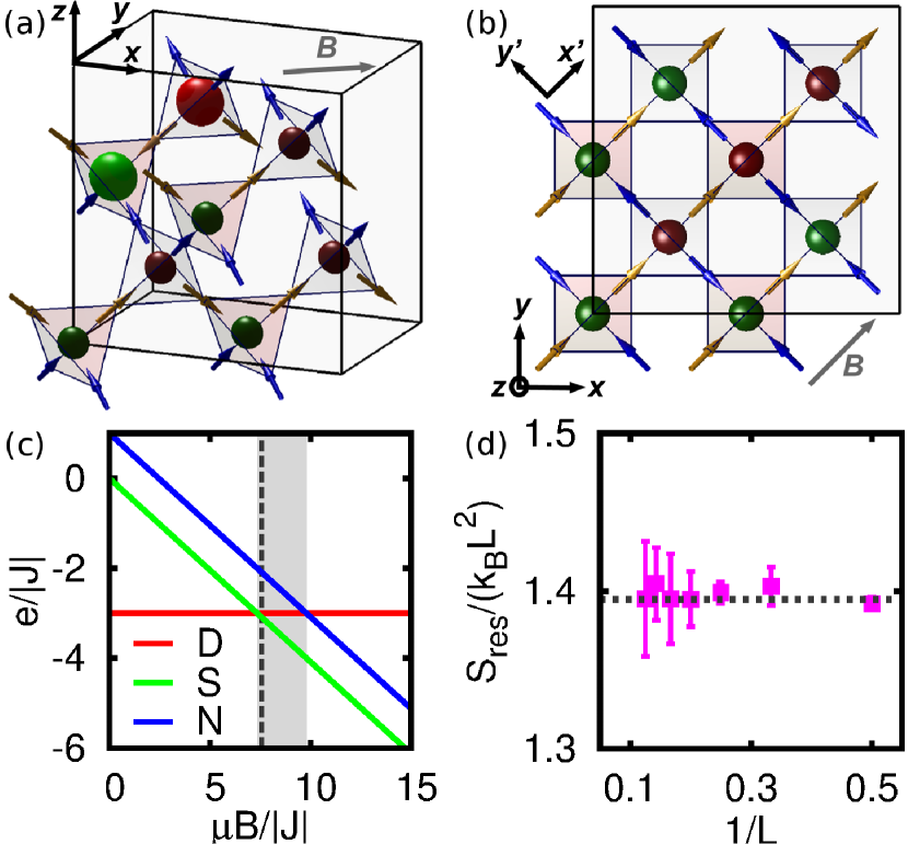
Figure 1: (a) Conventional unit cell of the pyrochlore lattice ($L=1$) with $4$ tetahedra pointing up (coloured) and $4$ pointing down (uncoloured). The arrows represent the spin direction at each site. The colour of the spheres marks the sign of the charges and the size is proportional to their modulus. (b) Planar projected configuration: a tetrahedron becomes a square with crossings, in a checkerboard lattice. The field ${\mathbf{B}}\parallel[110]$ couples to two spins on each tetrahedron ($\alpha$-chains, yellow arrows), and is orthogonal to the other two ($\beta$-chains, blue arrows). The configuration shown is a zero-temperature ground state for large fields. (c) The energy of a singly charged (S), doubly charged (D) and neutral tetrahedron (N) as functions of the magnetic energy normalised by the exchange energy scale; only the energies corresponding to the S and N configurations favoured by the field are shown. (d) Linear size dependence of the residual entropy $S_{\rm res}$.

Within the magnetic charge picture Castelnovo et al. (2008), the centres of up or down tetrahedra are considered neutral if two of their spins point in and two out, have a positive or negative single charge if three spins point in and one out or vice versa (pictured as small spheres in Fig. 1(a,b)), or a positive or negative double charge if all spins point in or all point out (pictured as big spheres in Fig. 1(a)). In this language, the ground state for ${\mathbf{B}}=0$ consists of an array of double charges of alternating sign with the zincblende structure, which spontaneously breaks the symmetry between the two FCC sublattices Guruciaga et al. (2014). Unlike the single charges and the neutral state, a double charge has no magnetic moment, making it unstable under a sufficiently strong magnetic field applied along any direction. ${\mathbf{B}}\parallel[110]$ is special in that it does so without favouring any FCC sublattice , opening the door to a single-charge disordered ground state. In order to measure the amount of charge order for a given spin configuration, we define the single and double staggered charge densities, $\rho_{S}^{s}$ and $\rho_{S}^{d}$ respectively. They represent the modulus of the magnetic charge density due to single or double monopoles in up tetrahedra, normalised so that full order corresponds to a value of 1. It is also useful to define $\rho_{S}=\rho_{S}^{s}+2\rho_{S}^{d}$ representing the total staggered charge per sublattice site.

As implied by Eq. (2), ${\mathbf{B}}$ lowers the energy of single charges and neutral tetrahedra with positive projection of magnetic moment along it, leaving that of double charges unchanged (see Fig. 1(c)). A field $B$ such that $\mu B/|J|>7.348$ stabilises a ground state which, while remaining globally neutral, has a single charge on each tetrahedron. This field orders the $\alpha$-chains ferromagnetically (Fig. 1(b)), isolating the $\beta$-chains in the same way that a $[111]$ field decouples the Kagomé planes in the spin ice case Sakakibara et al. (2003). Spins on $\beta$-chains are impervious to this field but not to the exchange interaction. Each $\beta$-chain will thus independently and spontaneously order antiferromagnetically (see Fig. 1(b)), implying a spontaneous one-dimensional staggered charge order along each $\beta$-chain. The additional freedom associated with the symmetry breaking within each separate $\beta$-chain means that no $3d$ staggered charge order can arise at $T=0$, though the residual entropy (proportional to the number of chains, not spins) is sub-extensive. We tested this fact using Monte Carlo (MC) simulations in a system of $L^{3}$ cubic cells and periodic boundary conditions with an applied field $\mu B/|J|=12.1$, well in the disordered regime. By integrating the specific heat over a wide temperature range $(0.1<k_{B}T/|J|<70)$, and through direct calculation from the density of states computed with the Wang-Landau (WL) algorithm Wang and Landau (2001), we obtained the residual entropy $S_{\rm res}\propto L^{2}$ for different system sizes (Fig. 1(d)). Details on the simulations are provided in the Supplemental Material sup .

Here we are interested in the situation in which the ground state consists of this disordered single-charge state while the lowest energy excitations correspond to double charges (see the shaded area in Fig. 1(c); the dashed line marks the field $\mu B/|J|=7.562$ used in the remainder of this work). The appearance of excitations implies an obvious entropy increase. On the other hand, their structure (all spins in, or all out) imposes nearest-neighbour correlations Guruciaga et al. (2014) that will favour charge order between adjoining chains, and thus the phenomenon of ObD that we will study.

The cluster variational method (CVM) places the tetrahedra on a tree with the same coordination number than the $3d$ lattice, i.e. four Levis et al. (2013); Foini et al. (2013); Cugliandolo et al. (2015) (Husimi tree). Once this is done, recurrence relations for the order parameters are derived and solved analytically in the infinite size limit. We tested the formation of charge order in the zincblende structure by measuring $\rho_{S}^{d}$ and $\rho_{S}^{s}$, plotted as continuous lines in Fig. 2. Within the CVM both order parameters are strictly zero at $T=0$. At an infinitesimal temperature $\rho_{S}^{s}$ jumps to one and $\rho_{S}^{d}$ increases continuously from zero. The two observables vanish at $T_{c}$ as in a second-order Ising-type phase transition with mean-field exponents. The specific heat at low $T$ has a standard Schottky anomaly due to two-level system excitations. The second peak indicates the transition to the disordered phase and it is just a cusp since $\alpha=0$ in mean-field. The MC simulations of the $3d$ model (symbols in Fig. 2) clearly support this interpretation of the specific heat, with a low temperature Schottky anomaly at low $T$, and a broad peak with evident FSE at $T_{c}$ (Fig. 2(c)). Its evolution with the number of spins $N$, as well as that of $\rho_{S}^{s}(T_{c})$ and its fluctuations, are consistent with a second-order transition within the $3d$ Ising universality class (see Supplemental Material sup ). In order to understand better the behaviour of the order parameter, we discuss the important low $T$ finite-size effects below.

A careful low-$T$ analysis is most easily implemented in the projection to the checkerboard lattice. As in the $3d$ case, the lowest energy levels are excited by flipping an $\alpha$-spin against $\bf{B}$. Furthermore, this $\alpha$-spin should link two $\beta$-chains with staggered AF $1d$ order. Labeling the spins $s_{ij}$ in Fig. 1(b) according to the coordinate system $(0;\,x,\,y)$, such an excitation would be to turn the spin $s_{22}$. This creates two defects with an energy cost equal to $2\epsilon=2\mu B-12J$ ($\epsilon/J=0.164$ for the parameters of the numerical simulations). For simplicity, we used open boundary conditions in this representation.

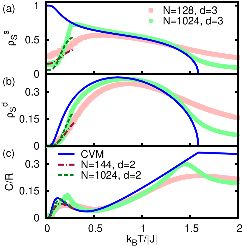
Figure 2: The order parameters (a) $\rho_{S}^{s}$ and (b) $\rho_{S}^{d}$, and (c) the specific heat as functions of temperature. The symbols show MC data for the $3d$ system and the dashed lines (with the same colour code) the results of the low-$T$ expansion for the $2d$ projection, both with similar number of spins $N$. The solid (blue) lines are the CVM outcome ($N\to\infty$).

With the exact enumeration of these excitations we calculated $\rho_{S}^{s}$ and $\rho_{S}^{d}$ for finite $N$ at low $T$. We expect the FSE to depend on the number of spins $N$ on the lattice, independently of its dimension $d$. We see in Fig. 2 that the behaviour observed for $d=2$ qualitatively follows that of the numerical simulations of the $3d$ system. The naive extrapolation of $\rho_{S}^{s}$ in the low $T$ limit for $N\to\infty$ suggests that $\rho_{S}^{s}$ vanishes in the thermodynamic limit, in seeming contradiction to the CVM results (top of Fig. 2). To explain this, we provide below a careful study of the interplay between the limits $N\to\infty$ and $\beta\epsilon\to\infty$ in the checkerboard model.

Consider two neighbouring $\beta$-chains with $M$ spins in the direction $y^{\prime}$ of the rotated coordinate system $(0;x^{\prime},y^{\prime})$ in Fig. 1(b) . In the low-$T$ limit the $\beta$-spins have perfect antiferromagnetic order along the$y^{\prime}$ direction. There are thus two possibilities for the relative orientation of the spins on neighbouring $\beta$-chains: either they are parallel (FM ordered, e.g., the second and third $\beta$-chains in Fig. 1(b)) or anti-parallel (AF ordered, e.g., in the first and second $\beta$-chain in Fig. 1(b)). In the latter case and for $M$ large enough there are $O(M/2)$ possible excitations of energy $2\epsilon$, obtained by reversing an $\alpha$-spin between the two $\beta$-chains, and the partition function is $Z_{AF}\simeq(1+e^{-2\beta\epsilon})^{M/2}$. In the former case there are no possible low-energy excitations (neglecting the presence of neutral tetrahedra) and $Z_{FM}\simeq 1$. This can be interpreted in terms of an effective AF coupling between the $\beta$-spins only. Let us compare the partition functions for the two possible orientations,

$$\frac{Z_{\rm AF}}{Z_{\rm FM}}=e^{-\beta(H^{\rm AF}_{\rm eff}-H^{\rm FM}_{\rm eff})}\;,\quad H_{\rm eff}=J_{\rm eff}\sum_{j^{\prime}=1}^{M}s^{\beta}_{1j^{\prime}}s^{\beta}_{2j^{\prime}}\;,$$ (3)

where $s^{\beta}_{i^{\prime}j^{\prime}}$ label the $\beta$-spins and $i^{\prime},j^{\prime}$ sweep the rotated lattice in Fig. 1(b). The interaction on each $\beta$-chain remains the original $J$. Then $H^{\rm AF}_{\rm eff}=-J_{\rm eff}M$, $H^{\rm FM}_{\rm eff}=J_{\rm eff}M$ and we conclude that $J_{\rm eff}$ is given by

$$J_{\rm eff}=(4\beta)^{-1}\ e^{-2\beta\epsilon}\;.$$ (4)

Thus, after integrating out the $\alpha$-spins, we have an effective low-$T$ model on a tilted $2d$ square lattice, with AF anisotropic interactions equal to $J$ in the $y^{\prime}$ direction and $J_{\rm eff}$ in the $x^{\prime}$ direction.

We now go one step further and we reduce the low-$T$ effective model to a $1d$ one. As mentioned, the $\beta$-chains are perfectly ordered for $k_{B}T/|J|\ll 1$. We define a macro $\beta$-spin $\sigma=+1$ ($-1$) according to the direction of the first spin on the chain being up (down). They sit on the sites of a $1d$ lattice and interact with an effective AF interaction $MJ_{\rm eff}$. The $T\to 0^{+}$ limit is then very tricky, since $J_{\rm eff}\to 0$ in a singular way. At any finite $M$, $MJ_{\rm eff}\to 0$ for $T\to 0^{+}$: the effective $1d$ system decouples and disorders. However, if we take $M\to\infty$ first, the effective $1d$ system orders AF and, as it was already AF ordered along the $\beta$-chains, it is fully AF-ordered with $\rho_{S}^{s}\xrightarrow[T\to 0^{+}]{}1$. In conclusion, the low-$T$ expansion predicts a first-order ObD transition with a finite jump of $\rho_{S}^{s}$ from zero to $1$, just as obtained with the CVM. One has

$$0=\lim_{N\to\infty}\lim_{T\to 0^{+}}\rho_{S}^{s}\neq\lim_{T\to 0^{+}}\lim_{N\to\infty}\rho_{S}^{s}=1\,.$$ (5)

MC results are not in contradiction with this: huge values of $N$ are needed to see a large $\rho_{S}^{s}$ as $T$ lowers (Fig. 2(a)).

ObD is sometimes illustrated by a cartoon Moessner (2001); Chalker (2011) in which the ground state manifold is represented by a curve in phase space (see Fig. 3(c$)$). The increment on the accessible phase space when raising $T$ slightly from $0$ is drawn as a surface (green) next to this curve. ObD occurs when the excitations linked to certain ordered ground states (cross) dominate the thermal average over all accessible states. We can turn this description into a quantitative argument by explicitly calculating the density of states $\delta(\Delta E,\rho_{S})$ of the $3d$ system with the WL algorithm. We move along the configuration space using two parameters: the energy excess with respect to the ground state, $\Delta E$, and the total staggered charge density, $\rho_{S}$. Figure 3 shows the low energy part of $\delta$ for $L=3$ and the same magnetic field used in Fig. 2. The colours emphasise the value of $\delta$, normalised using that there is a single state with $\rho_{S}=2$ (a double monopole crystal). Each point in the graph represents the real binning in energy and order parameter. We can see a very flat surface near the degenerate ground state energy ($\Delta E=0$) and two very noticeable symmetric peaks; e.g., at $\Delta E/(N|J|)=0.106$ the maxima are at $\rho_{S}^{\rm peak}\approx\pm 1.2$. Consistently, the MC canonical ensemble average of the order parameter and the one computed with

$$|\rho_{S}|^{\rm WL}=\frac{1}{{\cal Z}}\sum_{\Delta E_{k}}^{\Delta E_{k}^{\rm max}}\sum_{{\rho_{S}}_{l}}|{\rho_{S}}_{l}|\ \delta(\Delta E_{k},{\rho_{S}}_{l})\ e^{-\beta\Delta E_{k}}$$ (6)

with $\Delta E_{k}^{\rm max}/|J|=0.385$ coincide over a rather wide range of $T$, see Fig. 3(b). The remaining (pink) data-points are obtained as follows. We first read the density $\rho^{\rm peak}_{S}(\Delta E)$ that maximises $\delta$ for each $\Delta E$. Such an evaluation is quite precise on the interval $\Delta E/(N|J|)\in[0.05,0.2]$ and it coincides, within numerical accuracy, with $|\rho_{S}|(\langle\Delta E\rangle)$ measured with the MC or WL methods (not shown). We next transform the $\Delta E$ dependence into a $T$ dependence replacing $\Delta E$ by $\langle\Delta E\rangle(T)$ from the MC data. We therefore obtain $|\rho_{S}^{\rm peak}|(T)$ in Fig. 3(b). The good coincidence between the data points obtained in this way and through Eq. (6) marks the importance of low-energy thermal fluctuations around the ordered states. Furthermore, the procedure complements the low-$T$ expansion in the sense that it estimates $|\rho_{S}|$ beyond its maximum as a function of $T$.

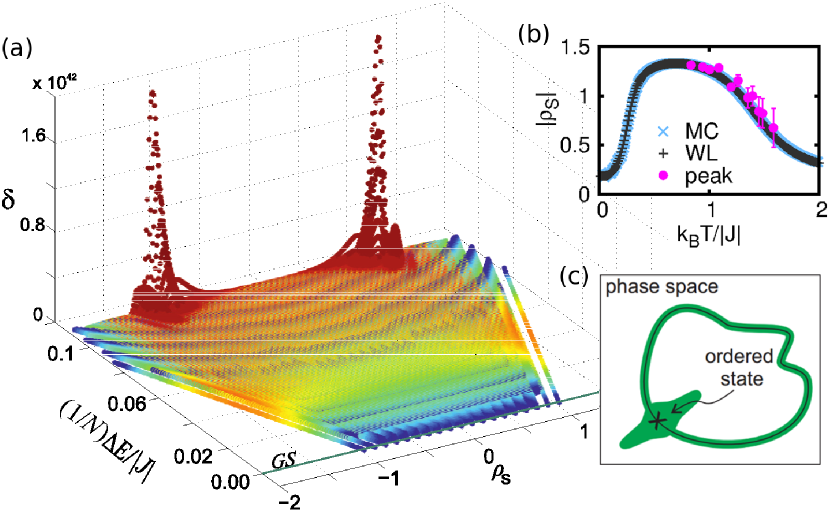
Figure 3: (a) Density of states $\delta$ as a function of excitation energy, $\Delta E$, and total staggered charge density, $\rho_{S}$, for a system of size $L=3$ and for $\mu B/|J|=7.562$. Each coloured circle corresponds to a single energy of the system. The two symmetric peaks are centered at $|\rho_{S}^{\rm peak}|\approx 1.2$. Inset (b) compares $|\rho_{S}|$ calculated from the WL method and the MC simulation with the values directly obtained from the maxima of $\delta$. Inset (c) –copied from Ref. Moessner (2001)– represents the ground state manifold (black curve) in parameter space, and the selection of an ordered state (cross) by thermal excitations (green region).

We will now discuss how an experimental contrast to our results may be possible with magnetic Reimers et al. (1991); Sadeghi et al. (2015); Anand et al. (2015); Xu et al. (2015); Marrows (2016) or colloidal Olson Reichhardt et al. (2012) samples. In order to observe classical ObD experimentally in these systems, the tendency towards a charge ordered ground state favoured by a misaligned ${\mathbf{B}}$ or long range dipolar interactions should be made as small as possible. A first option are the AF Ising pyrochlores Reimers et al. (1991); Sadeghi et al. (2015); Anand et al. (2015). They have the advantage that the stabilisation of the all-in–all-out state is achieved through the exchange interaction; this allows to keep the dipolar interaction small. Field misalignment can also be minimised by using a vector magnet Bruin et al. (2013). The observation of charge order at temperatures much higher than that characterising both the residual field and dipolar energy scales would be a strong indication of ObD. Detecting the AF order disappear as a function of increasing field (see Fig. 1(c)) would also be a conclusive smoking gun. Neutron scattering could be a sensitive probe if only short or medium range AF order is set due to competing ordering trends. A second route towards ObD is to take advantage of the recent advances in the design of frustrated magnets to create a planar system similar to the one in Fig. 1(b), thus minimising problems of field misalignment. The idea is to use artificial square-lattice spin-ice samples in their AF phase, with the vertex energy hierarchy $\epsilon_{\rm c}<\epsilon_{\rm e}<\epsilon_{\rm a,b}$ where ${\rm c}$ indicates AF, ${\rm e}$ three-in/one-out or three-out/one-in and ${\rm a,b}$ FM vertices Marrows (2016); Morgan et al. (2010) (see the Supplemental Material for a detailed explanation sup ). The third route concerns the use of colloidal systems in $2d$ arrays of optical traps, where staggered charge order could be attainable Olson Reichhardt et al. (2012); Ortíz-Ambriz and Tierno (2016). The precise control over the interactions and accessibility of thermal excitations may offer another fertile ground to recreate this experiment. As we have seen, FSE have a very strong influence in $\rho_{S}^{s}$; this fact may be exploited to recognise incipient ObD using samples with small size.

In summary, we have made an in-depth numerical and theoretical study of ObD in two models closely linked to ice systems. Our results may establish a route to the much sought-after experimental realisation of classical order-by-disorder.

I Simulation methods and further analysis

We provide here some details on the simulations used in the main text to study the equilibrium properties of nearest-neighbour antiferromagnetic Ising pyrochlores. We simulated $L\times L\times L$ conventional cubic cells of the pyrochlore lattice with periodic boundary conditions in the three directions with Metropolis and Wang-Landau Wang and Landau (2001) methods. In both cases we used a single-spin flip algorithm. In the Metropolis case, after reaching equilibrium we averaged the data over $10-150$ independent runs and $5\times 10^{4}-1.5\times 10^{6}$ time steps depending on temperature and lattice size. We have used a modified version of the Wang Landau Algorithm proposed by R. Bellardinelli and V. Pereyra Belardinelli and Pereyra (2007) to compute the density of states $\delta(\Delta E,\rho_{S})$ as a function of the order parameter $\rho_{S}$ and the excitation energy, restricting this last one to a range $\Delta E/(N|J|)=0.385$ from the ground state. The time-dependent modification factor changed from $e^{1}$ to $e^{10^{-7}}$ evolving as a function of the inverse of the Monte Carlo time. The final result is a relative density of state of the system. We used the condition $\delta(\rho_{s}=2)=1$ (where the addition over all energies is implied) to normalise it.

The main text is concerned with the order-by-disorder (ObD) process at low temperature; we now pay some attention to the high temperature feature (the usual “disorder-by-disorder” transition). In this case, while order is reinforced by the increasing number of double charges at higher $T$, the proliferation of neutral excitations has the opposite effect of decorrelating magnetic charges Guruciaga et al. (2014), thus disordering the system. To study this process, we performed a finite size analysis on systems with $L$ between $3$ and $20$ (a maximum of $128000$ spins). We show in Fig. 4 the single charge susceptibility $\chi_{S}^{s}$ (defined as the quadratic fluctuation of $\rho_{S}^{s}$ over temperature) in the temperature range of this transition. This quantity, as well as the specific heat $C$ and $\rho_{S}^{s}$ at the critical point, evolve with $L$ as in a second order phase transition (not shown). The critical exponents we observe are consistent with the three-dimensional Ising universality class (Fig. 4, inset).

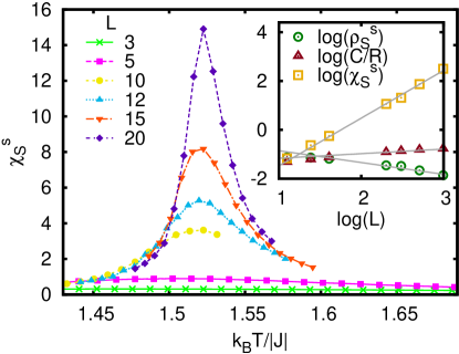
Figure 4: The single charge susceptibility $\chi_{S}^{s}$ displays finite size effects consistent with a second order phase transition. Inset: $\rho_{S}^{s}\left(T_{c}\left(L\right)\right)$, $C\left(T_{c}\left(L\right)\right)/R$ and $\chi_{S}^{s}\left(T_{c}\left(L\right)\right)$ evolve as power laws with the size of the system, and present good correspondence with the behavior expected for the three dimensional Ising model universality class (gray lines).

II Details on the antiferromagnetic ground state for the artificial spin ice

In this Supplemental Material we explain how ObD can be realized in artificial spin-ice (ASI) samples on planar square lattices. Differently from the three dimensional pyrochlores, deviations of the field orientation will not have drastic effects in these systems, making them suitable for the observation of thermal ObD.

ASI materials are made of arrays of elongated single-domain ferromagnetic nano-islands frustrated by dipolar interactions. The interaction parameters can be precisely engineered – by tuning the distance between islands, i.e. the lattice constant, or by applying external fields. These systems should set into different phases depending on the experimental conditions. Despite the irrelevance of temperature fluctuations, methods to equilibrate ASI up to quite low temperatures have been devised. Two of them are the gradual magneto-fluidization of an initially polarized state and the thermalization during the slow growth of the samples Morgan et al. (2010). Neglecting dipolar interactions between the magnetic islands, these systems can be described with the sixteen vertex model on a square lattice, with individual vertices shown and labeled as in Fig. 5 Levis et al. (2013); Foini et al. (2013).

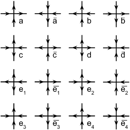
Figure 5: The sixteen vertices.

The idea is to engineer samples with the following (unusual but feasible Marrows (2016)) vertex energy hierarchy:

$$\epsilon_{\rm c}<\epsilon_{\rm e}<\epsilon_{\rm a,b}<\epsilon_{\rm d}\;.$$ (7)

The ground state of the system is the two-degenerate fully antiferromagnetic state, with alternating ${\rm c},\ \overline{\rm c}$ vertices. If one applies a magnetic field with magnitude $B$ in the $y$ direction, all vertices with vertical arrows pointing upwards decrease their energy (${\rm a},\ {\rm b},\ {\rm e}_{3},\ {\rm e}_{4}$), complementary all vertices with vertical arrows pointing downwards increase their energy ($\overline{\rm a},\ \overline{\rm b},\ \overline{\rm e}_{3},\ \overline{\rm e}_{4}$) while all other vertices are insensitive to this field. The vertex energy dependence on the field is sketched in Fig. 6. For $B>B^{*}$ the energies of the ${\rm e}_{3},\ {\rm e}_{4}$ vertices cross the ones of the ${\rm c},\ \overline{\rm c}$ vertices and the ground state becomes a disordered state made of ${\rm e}_{3},\ {\rm e}_{4}$ vertices. Indeed, all vertical arrows must point in the direction of the field. Therefore, each horizontal line is a sequence of alternating ${\rm e}_{3}$ and ${\rm e}_{4}$ vertices but there is no constraint on the way two consecutive horizontal lines order relative to each other. The number of ground states is proportional to $2^{L}$, with $L$ the number of lines.

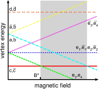
Figure 6: The dependence of the vertex energies on the applied magnetic field in the vertical direction. As in Fig. 1 in the main text, the shaded rectangle marks the field range where order-by-disorder would be expected.

If we choose a field with strength slightly larger than $B^{*}$, by the same mechanism explained in the main text, two ground states with staggered order between the horizontal lines (see Fig. 7 where one of them is shown) have a huge number of low energy excitations that correspond to flipping all the encircled vertical arrows that transform the ${\rm e}_{3}$ and ${\rm e}_{4}$ vertices into ${\rm c}$ and $\overline{\rm c}$ vertices. This feature produces an effective antiferromagnetic interaction between the horizontal spins that orders the system as soon as these excitation are activated by temperature. An effective one dimensional model can be derived for this problem following the same steps presented in the main text. Strong finite size effects are also present in this case and we propose to use them as a signature for ObD by analysing experimental data at low, but not so low, temperatures for moderate system sizes. Note that this scenario is not destroyed by a slight misalignment of the field. However, the dipolar interactions could lift the degeneracy between the ground states. Care must then be taken to make the dipolar interactions as weak as possible.

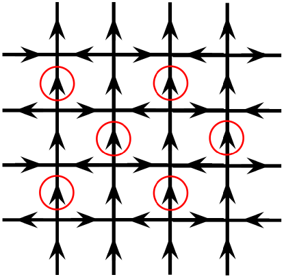
Figure 7: One of the two ground states with the most numerous low energy excitations. We indicate with circles the spins that could be flipped with the lowest energy cost, the only possible at very low temperatures.