Generative Topic Embedding: a Continuous Representation of Documents (Extended Version with Proofs)

Abstract

Word embedding maps words into a low-dimensional continuous embedding space by exploiting the local word collocation patterns in a small context window. On the other hand, topic modeling maps documents onto a low-dimensional topic space, by utilizing the global word collocation patterns in the same document. These two types of patterns are complementary. In this paper, we propose a generative topic embedding model to combine the two types of patterns. In our model, topics are represented by embedding vectors, and are shared across documents. The probability of each word is influenced by both its local context and its topic. A variational inference method yields the topic embeddings as well as the topic mixing proportions for each document. Jointly they represent the document in a low-dimensional continuous space. In two document classification tasks, our method performs better than eight existing methods, with fewer features. In addition, we illustrate with an example that our method can generate coherent topics even based on only one document.

1 Introduction

Representing documents as fixed-length feature vectors is important for many document processing algorithms. Traditionally documents are represented as a bag-of-words (BOW) vectors. However, this simple representation suffers from being high-dimensional and highly sparse, and loses semantic relatedness across the vector dimensions.

Word Embedding methods have been demonstrated to be an effective way to represent words as continuous vectors in a low-dimensional embedding space [Bengio et al., 2003, Mikolov et al., 2013, Pennington et al., 2014, Levy et al., 2015]. The learned embedding for a word encodes its semantic/syntactic relatedness with other words, by utilizing local word collocation patterns. In each method, one core component is the embedding link function, which predicts a word’s distribution given its context words, parameterized by their embeddings.

When it comes to documents, we wish to find a method to encode their overall semantics. Given the embeddings of each word in a document, we can imagine the document as a “bag-of-vectors”. Related words in the document point in similar directions, forming semantic clusters. The centroid of a semantic cluster corresponds to the most representative embedding of this cluster of words, referred to as the semantic centroids. We could use these semantic centroids and the number of words around them to represent a document.

In addition, for a set of documents in a particular domain, some semantic clusters may appear in many documents. By learning collocation patterns across the documents, the derived semantic centroids could be more topical and less noisy.

Topic Models, represented by Latent Dirichlet Allocation (LDA) [Blei et al., 2003], are able to group words into topics according to their collocation patterns across documents. When the corpus is large enough, such patterns reflect their semantic relatedness, hence topic models can discover coherent topics. The probability of a word is governed by its latent topic, which is modeled as a categorical distribution in LDA. Typically, only a small number of topics are present in each document, and only a small number of words have high probability in each topic. This intuition motivated ?) to regularize the topic distributions with Dirichlet priors.

Semantic centroids have the same nature as topics in LDA, except that the former exist in the embedding space. This similarity drives us to seek the common semantic centroids with a model similar to LDA. We extend a generative word embedding model PSDVec [Li et al., 2015], by incorporating topics into it. The new model is named TopicVec. In TopicVec, an embedding link function models the word distribution in a topic, in place of the categorical distribution in LDA. The advantage of the link function is that the semantic relatedness is already encoded as the cosine distance in the embedding space. Similar to LDA, we regularize the topic distributions with Dirichlet priors. A variational inference algorithm is derived. The learning process derives topic embeddings in the same embedding space of words. These topic embeddings aim to approximate the underlying semantic centroids.

To evaluate how well TopicVec represents documents, we performed two document classification tasks against eight existing topic modeling or document representation methods. Two setups of TopicVec outperformed all other methods on two tasks, respectively, with fewer features. In addition, we demonstrate that TopicVec can derive coherent topics based only on one document, which is not possible for topic models.

The source code of our implementation is available at https://github.com/askerlee/topicvec.

2 Related Work

?) proposed a generative word embedding method PSDVec, which is the precursor of TopicVec. PSDVec assumes that the conditional distribution of a word given its context words can be factorized approximately into independent log-bilinear terms. In addition, the word embeddings and regression residuals are regularized by Gaussian priors, reducing their chance of overfitting. The model inference is approached by an efficient Eigendecomposition and blockwise-regression method [Li et al., 2016]. TopicVec differs from PSDVec in that in the conditional distribution of a word, it is not only influenced by its context words, but also by a topic, which is an embedding vector indexed by a latent variable drawn from a Dirichlet-Multinomial distribution.

?) proposed to model topics as a certain number of binary hidden variables, which interact with all words in the document through weighted connections. ?) assigned each word a unique topic vector, which is a summarization of the context of the current word.

?) proposed to incorporate global (document-level) semantic information to help the learning of word embeddings. The global embedding is simply a weighted average of the embeddings of words in the document.

?) proposed Paragraph Vector. It assumes each piece of text has a latent paragraph vector, which influences the distributions of all words in this text, in the same way as a latent word. It can be viewed as a special case of TopicVec, with the topic number set to 1. Typically, however, a document consists of multiple semantic centroids, and the limitation of only one topic may lead to underfitting.

?) proposed Latent Feature Topic Modeling (LFTM), which extends LDA to incorporate word embeddings as latent features. The topic is modeled as a mixture of the conventional categorical distribution and an embedding link function. The coupling between these two components makes the inference difficult. They designed a Gibbs sampler for model inference. Their implementation is slow and infeasible when applied to a large corpous.

?) proposed Topical Word Embedding (TWE), which combines word embedding with LDA in a simple and effective way. They train word embeddings and a topic model separately on the same corpus, and then average the embeddings of words in the same topic to get the embedding of this topic. The topic embedding is concatenated with the word embedding to form the topical word embedding of a word. In the end, the topical word embeddings of all words in a document are averaged to be the embedding of the document. This method performs well on our two classification tasks. Weaknesses of TWE include: 1) the way to combine the results of word embedding and LDA lacks statistical foundations; 2) the LDA module requires a large corpus to derive semantically coherent topics.

?) proposed Gaussian LDA. It uses pre-trained word embeddings. It assumes that words in a topic are random samples from a multivariate Gaussian distribution with the topic embedding as the mean. Hence the probability that a word belongs to a topic is determined by the Euclidean distance between the word embedding and the topic embedding. This assumption might be improper as the Euclidean distance is not an optimal measure of semantic relatedness between two embeddings.

3 Notations and Definitions

Throughout this paper, we use uppercase bold letters such as $\boldsymbol{S},\boldsymbol{V}$ to denote a matrix or set, lowercase bold letters such as $\boldsymbol{v}_{w_{i}}$ to denote a vector, a normal uppercase letter such as $N,W$ to denote a scalar constant, and a normal lowercase letter as $s_{i},w_{i}$ to denote a scalar variable.

Table 1 lists the notations in this paper.

In a document, a sequence of words is referred to as a text window, denoted by $w_{i},\cdots,w_{i+l}$, or $w_{i}{:}w_{i+l}$. A text window of chosen size $c$ before a word $w_{i}$ defines the context of $w_{i}$ as $w_{i-c},\cdots,w_{i-1}$. Here $w_{i}$ is referred to as the focus word. Each context word $w_{i-j}$ and the focus word $w_{i}$ comprise a bigram $w_{i-j},w_{i}$.

Name	Description
$\boldsymbol{S}$	Vocabulary $\{s_{1},\cdots,s_{\scriptscriptstyle W}\}$
$\boldsymbol{V}$	Embedding matrix $(\boldsymbol{v}_{s_{1}},\cdots,\boldsymbol{v}_{s_{\scriptscriptstyle W}})$
$\boldsymbol{D}$	Document set $\{d_{1},\cdots,d_{\scriptscriptstyle M}\}$
$\boldsymbol{v}_{s_{i}}$	Embedding of word $s_{i}$
$a_{s_{i}s_{j}},\boldsymbol{A}$	Bigram residuals
$\boldsymbol{t}_{ik},\boldsymbol{T}_{i}$	Topic embeddings in doc $d_{i}$
$r_{ik},\boldsymbol{r}_{i}$	Topic residuals in doc $d_{i}$
$z_{ij}$	Topic assignment of the $j$-th word $j$ in doc $d_{i}$
$\boldsymbol{\phi}_{i}$	Mixing proportions of topics in doc $d_{i}$

Table 1: Table of notations

We assume each word in a document is semantically similar to a topic embedding. Topic embeddings reside in the same $N$-dimensional space as word embeddings. When it is clear from context, topic embeddings are often referred to as topics. Each document has $K$ candidate topics, arranged in the matrix form $\boldsymbol{T}_{i}=(\boldsymbol{t}_{i1}\cdots\boldsymbol{t}_{iK})$, referred to as the topic matrix. Specifically, we fix $\boldsymbol{t}_{i1}=\boldsymbol{0}$, referring to it as the null topic.

In a document $d_{i}$, each word $w_{ij}$ is assigned to a topic indexed by $z_{ij}\in\{1,\cdots,K\}$. Geometrically this means the embedding $\boldsymbol{v}_{w_{ij}}$ tends to align with the direction of $\boldsymbol{t}_{i,z_{ij}}$. Each topic $\boldsymbol{t}_{ik}$ has a document-specific prior probability to be assigned to a word, denoted as $\phi_{ik}=P(k|d_{i})$. The vector $\boldsymbol{\phi}_{i}=(\phi_{i1},\cdots,\phi_{iK})$ is referred to as the mixing proportions of these topics in document $d_{i}$.

4 Link Function of Topic Embedding

In this section, we formulate the distribution of a word given its context words and topic, in the form of a link function.

The core of most word embedding methods is a link function that connects the embeddings of a focus word and its context words, to define the distribution of the focus word. ?) proposed the following link function:

$$P(w_{c}\mid w_{0}:w_{c-1})$$

$$\approx P(w_{c})\exp\biggl{\{}\boldsymbol{v}_{w_{c}}^{\operatorname*{\scriptscriptstyle\top}}\sum_{l=0}^{c-1}\boldsymbol{v}_{w_{l}}+\sum_{l=0}^{c-1}a_{w_{l}w_{c}}\biggr{\}}.$$ (1)

Here $a_{w_{l}w_{c}}$ is referred as the bigram residual, indicating the non-linear part not captured by $\boldsymbol{v}_{w_{c}}^{\operatorname*{\scriptscriptstyle\top}}\boldsymbol{v}_{w_{l}}$. It is essentially the logarithm of the normalizing constant of a softmax term. Some literature, e.g. [Pennington et al., 2014], refers to such a term as a bias term.

(1) is based on the assumption that the conditional distribution $P(w_{c}\mid w_{0}:w_{c-1})$ can be factorized approximately into independent log-bilinear terms, each corresponding to a context word. This approximation leads to an efficient and effective word embedding algorithm PSDVec [Li et al., 2015]. We follow this assumption, and propose to incorporate the topic of $w_{c}$ in a way like a latent word. In particular, in addition to the context words, the corresponding embedding $\boldsymbol{t}_{ik}$ is included as a new log-bilinear term that influences the distribution of $w_{c}$. Hence we obtain the following extended link function:[-0.5em]0em

$$\>P(w_{c}\mid w_{0}{:}w_{c-1},z_{c},d_{i})\approx P(w_{c})\cdot$$

$$\exp\Bigl{\{}\boldsymbol{v}_{w_{c}}^{\operatorname*{\scriptscriptstyle\top}}\Bigl{(}\sum_{l=0}^{c-1}\boldsymbol{v}_{w_{l}}+\boldsymbol{t}_{z_{c}}\Bigr{)}\negmedspace+\negmedspace\sum_{l=0}^{c-1}a_{w_{l}w_{c}}\negmedspace+\negmedspace r_{z_{c}}\Bigr{\}},$$ (2)

where $d_{i}$ is the current document, and $r_{z_{c}}$ is the logarithm of the normalizing constant, named the topic residual. Note that the topic embeddings $\boldsymbol{t}_{z_{c}}$ may be specific to $d_{i}$. For simplicity of notation, we drop the document index in $\boldsymbol{t}_{z_{c}}$. To restrict the impact of topics and avoid overfitting, we constrain the magnitudes of all topic embeddings, so that they are always within a hyperball of radius $\gamma$.

It is infeasible to compute the exact value of the topic residual $r_{k}$. We approximate it by the context size $c=0$. Then (2) becomes:

$$P(w_{c}\mid k,d_{i})=P(w_{c})\exp\left\{\boldsymbol{v}_{w_{c}}^{\operatorname*{\scriptscriptstyle\top}}\boldsymbol{t}_{k}+r_{k}\right\}.$$ (3)

It is required that $\sum_{w_{c}\in\boldsymbol{S}}P(w_{c}\mid k)=1$ to make (3) a distribution. It follows that

$$r_{k}=-\log\Bigl{(}\sum_{s_{j}\in\boldsymbol{S}}P(s_{j})\exp\{\boldsymbol{v}_{s_{j}}^{\operatorname*{\scriptscriptstyle\top}}\boldsymbol{t}_{k}\}\Bigr{)}.$$ (4)

(4) can be expressed in the matrix form:

$$\boldsymbol{r}=-\log(\boldsymbol{u}\exp\{\boldsymbol{V}^{\operatorname*{\scriptscriptstyle\top}}\boldsymbol{T}\}),$$ (5)

where $\boldsymbol{u}$ is the row vector of unigram probabilities.

[-1em]0em

Figure 1: Graphical representation of TopicVec.

5 Generative Process and Likelihood

The generative process of words in documents can be regarded as a hybrid of LDA and PSDVec. Analogous to PSDVec, the word embedding $\boldsymbol{v}_{s_{i}}$ and residual $a_{s_{i}s_{j}}$ are drawn from respective Gaussians. For the sake of clarity, we ignore their generation steps, and focus on the topic embeddings. The remaining generative process is as follows:

1. For the $k$-th topic, draw a topic embedding uniformly from a hyperball of radius $\gamma$, i.e. $\boldsymbol{t}_{k}\sim\textrm{Unif}(B_{\gamma})$;

2. For each document $d_{i}$:

   1. Draw the mixing proportions $\boldsymbol{\phi}_{i}$ from the Dirichlet prior $\textrm{Dir}(\boldsymbol{\alpha})$;

   2. For the $j$-th word:

      1. Draw topic assignment $z_{ij}$ from the categorical distribution Cat$(\boldsymbol{\phi}_{i})$;

      2. Draw word $w_{ij}$ from $\boldsymbol{S}$ according to $P(w_{ij}\mid w_{i,j-c}{:}w_{i,j-1},z_{ij},d_{i})$.

The above generative process is presented in plate notation in Figure (1).

5.1 Likelihood Function

Given the embeddings $\boldsymbol{V}$, the bigram residuals $\boldsymbol{A}$, the topics $\boldsymbol{T}_{i}$ and the hyperparameter $\boldsymbol{\alpha}$, the complete-data likelihood of a single document $d_{i}$ is:

$$p(d_{i},\boldsymbol{Z}_{i},\boldsymbol{\phi}_{i}|\boldsymbol{\alpha},\boldsymbol{V},\boldsymbol{A},\boldsymbol{T}_{i})$$

$$= p(\boldsymbol{\phi}_{i}|\boldsymbol{\alpha})p(\boldsymbol{Z}_{i}|\boldsymbol{\phi}_{i})p(d_{i}|\boldsymbol{V},\boldsymbol{A},\boldsymbol{T}_{i},\boldsymbol{Z}_{i})$$

$$= \frac{\Gamma(\sum_{k=1}^{K}\alpha_{k})}{\prod_{k=1}^{K}\Gamma(\alpha_{k})}\prod_{j=1}^{K}\phi_{ij}^{\alpha_{j}-1}\cdot\prod_{j=1}^{L_{i}}\Bigg{(}\phi_{i,z_{ij}}P(w_{ij})$$

$$\cdot\exp\biggl{\{}\boldsymbol{v}_{w_{ij}}^{\operatorname*{\scriptscriptstyle\top}}\Bigl{(}\sum_{l=j-c}^{j-1}\boldsymbol{v}_{w_{il}}+\boldsymbol{t}_{z_{ij}}\Bigr{)}$$

$$+\negthickspace\sum_{l=j-c}^{j-1}a_{w_{il}w_{ij}}\negmedspace+r_{i,z_{ij}}\biggr{\}}\Bigg{)},$$ (6)

where $\boldsymbol{Z}_{i}=(z_{i1},\cdots,z_{iL_{i}})$, and $\Gamma(\cdot)$ is the Gamma function.

Let $\boldsymbol{Z},\boldsymbol{T},\boldsymbol{\phi}$ denote the collection of all the document-specific $\{\boldsymbol{Z}_{i}\}_{i=1}^{M},\{\boldsymbol{T}_{i}\}_{i=1}^{M},\{\boldsymbol{\phi}_{i}\}_{i=1}^{M}$, respectively. Then the complete-data likelihood of the whole corpus is:

$$p(\boldsymbol{D},\boldsymbol{A},\boldsymbol{V},\boldsymbol{Z},\boldsymbol{T},\boldsymbol{\phi}|\boldsymbol{\alpha},\gamma,\boldsymbol{\mu})$$

$$= \prod_{i=1}^{W}P(\boldsymbol{v}_{s_{i}};\mu_{i})\prod_{i,j=1}^{W,W}P(a_{s_{i}s_{j}};f(h_{ij}))\prod_{k}^{K}\textrm{Unif}(B_{\gamma})$$

$$\cdot\prod_{i=1}^{M}\left\{p(\boldsymbol{\phi}_{i}|\boldsymbol{\alpha})p(\boldsymbol{Z}_{i}|\boldsymbol{\phi}_{i})p(d_{i}|\boldsymbol{V},\boldsymbol{A},\boldsymbol{T}_{i},\boldsymbol{Z}_{i})\right\}$$

$$= \frac{1}{\mathcal{Z}(\boldsymbol{H},\boldsymbol{\mu})U_{\gamma}^{K}}\exp\{-\negmedspace\sum_{i,j=1}^{W,W}f(h_{i,j})a_{s_{i}s_{j}}^{2}\negmedspace-\negmedspace\sum_{i=1}^{W}\mu_{i}\|\boldsymbol{v}_{s_{i}}\|^{2}\}$$

$$\cdot\prod_{i=1}^{M}\biggl{\{}\frac{\Gamma(\sum_{k=1}^{K}\alpha_{k})}{\prod_{k=1}^{K}\Gamma(\alpha_{k})}\prod_{j=1}^{K}\phi_{ij}^{\alpha_{j}-1}\cdot\prod_{j=1}^{L_{i}}\biggl{(}\phi_{i,z_{ij}}P(w_{ij})$$

$$\cdot\exp\Bigl{\{}\boldsymbol{v}_{w_{ij}}^{\operatorname*{\scriptscriptstyle\top}}\Bigl{(}\sum_{l=j-c}^{j-1}\boldsymbol{v}_{w_{il}}\negmedspace+\negmedspace\boldsymbol{t}_{z_{ij}}\Bigr{)}\negmedspace+\negmedspace\negthickspace\sum_{l=j-c}^{j-1}\negmedspace a_{w_{il}w_{ij}}\negmedspace+\negmedspace r_{i,z_{ij}}\negmedspace\Bigr{\}}\negmedspace\biggr{)}\negmedspace\biggr{\}},$$ (7)

where $P(\boldsymbol{v}_{s_{i}};\mu_{i})$ and $P(a_{s_{i}s_{j}};f(h_{ij}))$ are the two Gaussian priors as defined in [Li et al., 2015]. Following the convention in [Li et al., 2015], $h_{ij},\boldsymbol{H}$ are empirical bigram probabilities, $\boldsymbol{\mu}$ are the embedding magnitude penalty coefficients, and $\mathcal{Z}(\boldsymbol{H},\boldsymbol{\mu})$ is the normalizing constant for word embeddings. $U_{\gamma}$ is the volume of the hyperball of radius $\gamma$.

Taking the logarithm of both sides, we obtain

$$\log p(\boldsymbol{D},\boldsymbol{A},\boldsymbol{V},\boldsymbol{Z},\boldsymbol{T},\boldsymbol{\phi}|\boldsymbol{\alpha},\gamma,\boldsymbol{\mu})$$

$$= C_{0}-\log\mathcal{Z}(\boldsymbol{H},\boldsymbol{\mu})-\|\boldsymbol{A}\|_{f(\boldsymbol{H})}^{2}-\sum_{i=1}^{W}\mu_{i}\|\boldsymbol{v}_{s_{i}}\|^{2}$$

$$+ \sum_{i=1}^{M}\biggl{\{}\sum_{k=1}^{K}\log\phi_{ik}(m_{ik}+\alpha_{k}-1)+\sum_{j=1}^{L_{i}}\biggl{(}r_{i,z_{ij}}$$

$$+ \boldsymbol{v}_{w_{ij}}^{\operatorname*{\scriptscriptstyle\top}}\Bigl{(}\sum_{l=j-c}^{j-1}\boldsymbol{v}_{w_{il}}+\boldsymbol{t}_{z_{ij}}\Bigr{)}+\negthickspace\sum_{l=j-c}^{j-1}\negthickspace a_{w_{il}w_{ij}}\biggr{)}\negthickspace\biggr{\}},$$ (8)

where $m_{ik}=\sum_{j=1}^{L_{i}}\delta(z_{ij}=k)$ counts the number of words assigned with the $k$-th topic in $d_{i}$, $C_{0}=M\log\frac{\Gamma(\sum_{k=1}^{K}\alpha_{k})}{\prod_{k=1}^{K}\Gamma(\alpha_{k})}+\sum_{i,j=1}^{M,L_{i}}\log P(w_{ij})-K\log U_{\gamma}$ is constant given the hyperparameters.

6 Variational Inference Algorithm

6.1 Learning Objective and Process

Given the hyperparameters $\boldsymbol{\alpha},\gamma,\boldsymbol{\mu}$, the learning objective is to find the embeddings $\boldsymbol{V}$, the topics $\boldsymbol{T}$, and the word-topic and document-topic distributions $p(\boldsymbol{Z}_{i},\boldsymbol{\phi}_{i}|d_{i},\boldsymbol{A},\boldsymbol{V},\boldsymbol{T})$. Here the hyperparameters $\boldsymbol{\alpha},\gamma,\boldsymbol{\mu}$ are kept constant, and we make them implicit in the distribution notations.

However, the coupling between $\boldsymbol{A},\boldsymbol{V}$ and $\boldsymbol{T},\boldsymbol{Z},\boldsymbol{\phi}$ makes it inefficient to optimize them simultaneously. To get around this difficulty, we learn word embeddings and topic embeddings separately. Specifically, the learning process is divided into two stages:

1. In the first stage, considering that the topics have a relatively small impact to word distributions and the impact might be “averaged out” across different documents, we simplify the model by ignoring topics temporarily. Then the model falls back to the original PSDVec. The optimal solution $\boldsymbol{V}^{*},\boldsymbol{A}^{*}$ is obtained accordingly;

2. In the second stage, we treat $\boldsymbol{V}^{*},\boldsymbol{A}^{*}$ as constant, plug it into the likelihood function, and find the corresponding optimal $\boldsymbol{T}^{*},p(\boldsymbol{Z},\boldsymbol{\phi}|\boldsymbol{D},\boldsymbol{A}^{*},\boldsymbol{V}^{*},\boldsymbol{T}^{*})$ of the full model. As in LDA, this posterior is analytically intractable, and we use a simpler variational distribution $q(\boldsymbol{Z},\boldsymbol{\phi})$ to approximate it.

6.2 Mean-Field Approximation and Variational GEM Algorithm

In this stage, we fix $\boldsymbol{V}=\boldsymbol{V}^{*},\boldsymbol{A}=\boldsymbol{A}^{*}$, and seek the optimal $\boldsymbol{T}^{*},p(\boldsymbol{Z},\boldsymbol{\phi}|\boldsymbol{D},\boldsymbol{A}^{*},\boldsymbol{V}^{*},\boldsymbol{T}^{*})$. As $\boldsymbol{V}^{*},\boldsymbol{A}^{*}$ are constant, we also make them implicit in the following expressions.

For an arbitrary variational distribution $q(\boldsymbol{Z},\boldsymbol{\phi})$, the following equalities hold

$$E_{q}\log\left[\frac{p(\boldsymbol{D},\boldsymbol{Z},\boldsymbol{\phi}|\boldsymbol{T})}{q(\boldsymbol{Z},\boldsymbol{\phi})}\right]$$

$$= E_{q}\left[\log p(\boldsymbol{D},\boldsymbol{Z},\boldsymbol{\phi}|\boldsymbol{T})\right]+\mathcal{H}(q)$$

$$= \log p(\boldsymbol{D}|\boldsymbol{T})-\textrm{KL}(q||p),$$ (9)

where $p=p(\boldsymbol{Z},\boldsymbol{\phi}|\boldsymbol{D},\boldsymbol{T})$, $\mathcal{H}(q)$ is the entropy of $q$. This implies

$$\textrm{KL}(q||p)$$

$$= \log p(\boldsymbol{D}|\boldsymbol{T})-\Bigl{(}E_{q}\left[\log p(\boldsymbol{D},\boldsymbol{Z},\boldsymbol{\phi}|\boldsymbol{T})\right]+\mathcal{H}(q)\Bigr{)}$$

$$= \log p(\boldsymbol{D}|\boldsymbol{T})-\mathcal{L}(q,\boldsymbol{T}).$$ (10)

In (10), $E_{q}\left[\log p(\boldsymbol{D},\boldsymbol{Z},\boldsymbol{\phi}|\boldsymbol{T})\right]+\mathcal{H}(q)$ is usually referred to as the variational free energy $\mathcal{L}(q,\boldsymbol{T})$, which is a lower bound of $\log p(\boldsymbol{D}|\boldsymbol{T})$. Directly maximizing $\log p(\boldsymbol{D}|\boldsymbol{T})$ w.r.t. $\boldsymbol{T}$ is intractable due to the hidden variables $\boldsymbol{Z},\boldsymbol{\phi}$, so we maximize its lower bound $\mathcal{L}(q,\boldsymbol{T})$ instead. We adopt a mean-field approximation of the true posterior as the variational distribution, and use a variational algorithm to find $q^{*},\boldsymbol{T}^{*}$ maximizing $\mathcal{L}(q,\boldsymbol{T})$.

The following variational distribution is used:

$$q(\boldsymbol{Z},\boldsymbol{\phi};\boldsymbol{\pi},\boldsymbol{\theta})=q(\boldsymbol{\phi};\boldsymbol{\theta})q(\boldsymbol{Z};\boldsymbol{\pi})$$

$$= \prod_{i=1}^{M}\left\{\textrm{Dir}(\boldsymbol{\phi}_{i};\boldsymbol{\theta}_{i})\prod_{j=1}^{L_{i}}\textrm{Cat}(z_{ij};\boldsymbol{\pi}_{ij})\right\}.$$ (11)

We can obtain (Appendix A)

$$\mathcal{L}(q,\boldsymbol{T})$$

$$= \sum_{i=1}^{M}\Biggl{\{}\sum_{k=1}^{K}\Bigl{(}\sum_{j=1}^{L_{i}}\pi_{ij}^{k}+\alpha_{k}-1\Bigr{)}\Bigl{(}\psi(\theta_{ik})-\psi(\theta_{i0})\Bigr{)}$$

$$+\textrm{Tr}(\boldsymbol{T}_{i}^{\operatorname*{\scriptscriptstyle\top}}\sum_{j=1}^{L_{i}}\boldsymbol{v}_{w_{ij}}\boldsymbol{\pi}_{ij}^{\operatorname*{\scriptscriptstyle\top}})+\boldsymbol{r}_{i}^{\operatorname*{\scriptscriptstyle\top}}\sum_{j=1}^{L_{i}}\boldsymbol{\pi}_{ij}\Biggr{\}}$$

$$+\mathcal{H}(q)+C_{1},$$ (12)

where $\boldsymbol{T}_{i}$ is the topic matrix of the $i$-th document, and $\boldsymbol{r}_{i}$ is the vector constructed by concatenating all the topic residuals $r_{ik}$. $C_{1}=C_{0}-\log\mathcal{Z}(\boldsymbol{H},\boldsymbol{\mu})-\|\boldsymbol{A}\|_{f(\boldsymbol{H})}^{2}-\sum_{i=1}^{W}\mu_{i}\|\boldsymbol{v}_{s_{i}}\|^{2}+\sum_{i,j=1}^{M,L_{i}}\Bigl{(}\boldsymbol{v}_{w_{ij}}^{\operatorname*{\scriptscriptstyle\top}}\sum_{k=j-c}^{j-1}\boldsymbol{v}_{w_{ik}}+\sum_{k=j-c}^{j-1}a_{w_{ik}w_{ij}}\Bigr{)}$ is constant.

We proceed to optimize (12) with a Generalized Expectation-Maximization (GEM) algorithm w.r.t. $q$ and $\boldsymbol{T}$ as follows:

1. Initialize all the topics $\boldsymbol{T}_{i}=\boldsymbol{0}$, and correspondingly their residuals $\boldsymbol{r}_{i}=\boldsymbol{0}$;

2. Iterate over the following two steps until convergence. In the $l$-th step:

   1. Let the topics and residuals be $\boldsymbol{T}=\boldsymbol{T}^{(l-1)},\boldsymbol{r}=\boldsymbol{r}^{(l-1)}$, find $q^{(l)}(\boldsymbol{Z},\boldsymbol{\phi})$ that maximizes $\mathcal{L}(q,\boldsymbol{T}^{(l-1)})$. This is the Expectation step (E-step). In this step, $\log p(\boldsymbol{D}|\boldsymbol{T})$ is constant. Then the $q$ that maximizes $\mathcal{L}(q,\boldsymbol{T}^{(l)})$ will minimize $\textrm{KL}(q||p)$, i.e. such a $q$ is the closest variational distribution to $p$ measured by KL-divergence;

   2. Given the variational distribution $q^{(l)}(\boldsymbol{Z},\boldsymbol{\phi})$, find $\boldsymbol{T}^{(l)},\boldsymbol{r}^{(l)}$ that improve $\mathcal{L}(q^{(l)},\boldsymbol{T})$, using Gradient descent method. This is the generalized Maximization step (M-step). In this step, $\boldsymbol{\pi},\boldsymbol{\theta},\mathcal{H}(q)$ are constant.

6.2.1 Update Equations of $\boldsymbol{\pi},\boldsymbol{\theta}$ in E-Step

In the E-step, $\boldsymbol{T}=\boldsymbol{T}^{(l-1)},\boldsymbol{r}=\boldsymbol{r}^{(l-1)}$ are constant. Taking the derivative of $\mathcal{L}(q,\boldsymbol{T}^{(l-1)})$ w.r.t. $\pi_{ij}^{k}$ and $\theta_{ik}$, respectively, we can obtain the optimal solutions (Appendix B) at:

$$\pi_{ij}^{k} \propto\exp\{\psi(\theta_{ik})+\boldsymbol{v}_{w_{ij}}^{\operatorname*{\scriptscriptstyle\top}}\boldsymbol{t}_{ik}+r_{ik}\}.$$ (13)

$$\theta_{ik} =\sum_{j=1}^{L_{i}}\pi_{ij}^{k}+\alpha_{k}.$$ (14)

6.2.2 Update Equation of $\boldsymbol{T}_{i}$ in M-Step

In the Generalized M-step, $\boldsymbol{\pi}=\boldsymbol{\pi}^{(l)},\boldsymbol{\theta}=\boldsymbol{\theta}^{(l)}$ are constant. For notational simplicity, we drop their superscripts $(l)$.

To update $\boldsymbol{T}_{i}$, we first take the derivative of (12) w.r.t. $\boldsymbol{T}_{i}$, and then take the Gradient Descent method.

The derivative is obtained as (Appendix C):

$$\frac{\partial\mathcal{L}(q^{(l)},\boldsymbol{T})}{\partial\boldsymbol{T}_{i}}$$

$$= \sum_{j=1}^{L_{i}}\boldsymbol{v}_{w_{ij}}\boldsymbol{\pi}_{ij}^{\operatorname*{\scriptscriptstyle\top}}+\sum_{k=1}^{K}\bar{m}_{ik}\frac{\partial r_{ik}}{\partial\boldsymbol{T}_{i}},$$ (15)

where $\bar{m}_{ik}=\sum_{j=1}^{L_{i}}\pi_{ij}^{k}=E[m_{ik}]$, the sum of the variational probabilities of each word being assigned to the $k$-th topic in the $i$-th document. $\frac{\partial r_{ik}}{\partial\boldsymbol{T}_{i}}$ is a gradient matrix, whose $j$-th column is $\frac{\partial r_{ik}}{\partial\boldsymbol{t}_{ij}}$.

Remind that $r_{ik}=-\log\Bigl{(}E_{P(s)}[\exp\{\boldsymbol{v}_{s}^{\operatorname*{\scriptscriptstyle\top}}\boldsymbol{t}_{ik}\}]\Bigr{)}$. When $j\neq k$, it is easy to verify that $\frac{\partial r_{ik}}{\partial\boldsymbol{t}_{ij}}=\boldsymbol{0}$. When $j=k$, we have

$$\frac{\partial r_{ik}}{\partial\boldsymbol{t}_{ik}} =e^{-r_{ik}}\cdot E_{P(s)}[\exp\{\boldsymbol{v}_{s}^{\operatorname*{\scriptscriptstyle\top}}\boldsymbol{t}_{ik}\}\boldsymbol{v}_{s}]$$

$$=e^{-r_{ik}}\cdot\sum_{s\in W}\exp\{\boldsymbol{v}_{s}^{\operatorname*{\scriptscriptstyle\top}}\boldsymbol{t}_{ik}\}P(s)\boldsymbol{v}_{s}$$

$$=e^{-r_{ik}}\cdot\exp\{\boldsymbol{t}_{ik}^{\operatorname*{\scriptscriptstyle\top}}\boldsymbol{V}\}(\boldsymbol{u}\circ\boldsymbol{V}),$$ (16)

where $\boldsymbol{u}\circ\boldsymbol{V}$ is to multiply each column of $\boldsymbol{V}$ with $\boldsymbol{u}$ element-by-element.

Therefore $\frac{\partial r_{ik}}{\partial\boldsymbol{T}_{i}}=(\boldsymbol{0},\cdots\frac{\partial r_{ik}}{\partial\boldsymbol{t}_{ik}},\cdots,\boldsymbol{0})$. Plugging it into (15), we obtain

$$\frac{\partial\mathcal{L}(q^{(l)},\boldsymbol{T})}{\partial\boldsymbol{T}_{i}}=\sum_{j=1}^{L_{i}}\boldsymbol{v}_{w_{ij}}\boldsymbol{\pi}_{ij}^{\operatorname*{\scriptscriptstyle\top}}+(\bar{m}_{i1}\frac{\partial r_{i1}}{\partial\boldsymbol{t}_{i1}},\cdots,\bar{m}_{iK}\frac{\partial r_{iK}}{\partial\boldsymbol{t}_{iK}}).$$

We proceed to optimize $\boldsymbol{T}_{i}$ with a gradient descent method:

$$\boldsymbol{T}_{i}^{(l)}=\boldsymbol{T}^{(l-1)}+\lambda(l,L_{i})\frac{\partial\mathcal{L}(q^{(l)},\boldsymbol{T})}{\partial\boldsymbol{T}_{i}},$$

where $\lambda(l,L_{i})=\frac{L_{0}\lambda_{0}}{l\cdot\max\{L_{i},L_{0}\}}$ is the learning rate function, $L_{0}$ is a pre-specified document length threshold, and $\lambda_{0}$ is the initial learning rate. As the magnitude of $\frac{\partial\mathcal{L}(q^{(l)},\boldsymbol{T})}{\partial\boldsymbol{T}_{i}}$ is approximately proportional to the document length $L_{i}$, to avoid the step size becoming too big a on a long document, if $L_{i}>L_{0}$, we normalize it by $L_{i}$.

To satisfy the constraint that $\|\boldsymbol{t}_{ik}^{(l)}\|\leq\gamma$, when $\boldsymbol{t}_{ik}^{(l)}>\gamma$, we normalize it by $\gamma/\|\boldsymbol{t}_{ik}^{(l)}\|$.

After we obtain the new $\boldsymbol{T}$, we update $\boldsymbol{r}_{i}^{(m)}$ using (5).

Sometimes, especially in the initial several iterations, due to the excessively big step size of the gradient descent, $\mathcal{L}(q,\boldsymbol{T})$ may decrease after the update of $\boldsymbol{T}$. Nonetheless the general direction of $\mathcal{L}(q,\boldsymbol{T})$ is increasing.

6.3 Sharing of Topics across Documents

In principle we could use one set of topics across the whole corpus, or choose different topics for different subsets of documents. One could choose a way to best utilize cross-document information.

For instance, when the document category information is available, we could make the documents in each category share their respective set of topics, so that $M$ categories correspond to $M$ sets of topics. In the learning algorithm, only the update of $\pi_{ij}^{k}$ needs to be changed to cater for this situation: when the $k$-th topic is relevant to the document $i$, we update $\pi_{ij}^{k}$ using (13); otherwise $\pi_{ij}^{k}=0$.

An identifiability problem may arise when we split topic embeddings according to document subsets. In different topic groups, some highly similar redundant topics may be learned. If we project documents into the topic space, portions of documents in the same topic in different documents may be projected onto different dimensions of the topic space, and similar documents may eventually be projected into very different topic proportion vectors. In this situation, directly using the projected topic proportion vectors could cause problems in unsupervised tasks such as clustering. A simple solution to this problem would be to compute the pairwise similarities between topic embeddings, and consider these similarities when computing the similarity between two projected topic proportion vectors. Two similar documents will then still receive a high similarity score.

7 Experimental Results

To investigate the quality of document representation of our TopicVec model, we compared its performance against eight topic modeling or document representation methods in two document classification tasks. Moreover, to show the topic coherence of TopicVec on a single document, we present the top words in top topics learned on a news article.

7.1 Document Classification Evaluation

7.1.1 Experimental Setup

Compared Methods  Two setups of TopicVec were evaluated:

• TopicVec: the topic proportions learned by TopicVec;

• TV+MeanWV: the topic proportions, concatenated with the mean word embedding of the document (same as the MeanWV below).

We compare the performance of our methods against eight methods, including three topic modeling methods, three continuous document representation methods, and the conventional bag-of-words (BOW) method. The count vector of BOW is unweighted.

The topic modeling methods include:

• LDA: the vanilla LDA [Blei et al., 2003] in the gensim library;

• sLDA: Supervised Topic Model [McAuliffe and Blei, 2008], which improves the predictive performance of LDA by modeling class labels;

• LFTM: Latent Feature Topic Modeling [Nguyen et al., 2015].

The document-topic proportions of topic modeling methods were used as their document representation.

The document representation methods are:

• Doc2Vec: Paragraph Vector [Le and Mikolov, 2014] in the gensim library.

• TWE: Topical Word Embedding [Liu et al., 2015], which represents a document by concatenating average topic embedding and average word embedding, similar to our TV+MeanWV;

• GaussianLDA: Gaussian LDA [Das et al., 2015], which assumes that words in a topic are random samples from a multivariate Gaussian distribution with the mean as the topic embedding. Similar to TopicVec, we derived the posterior topic proportions as the features of each document;

• MeanWV: The mean word embedding of the document.

Datasets  We used two standard document classification corpora: the 20 Newsgroups and the ApteMod version of the Reuters-21578 corpus. The two corpora are referred to as the 20News and Reuters in the following.

20News contains about 20,000 newsgroup documents evenly partitioned into 20 different categories. Reuters contains 10,788 documents, where each document is assigned to one or more categories. For the evaluation of document classification, documents appearing in two or more categories were removed. The numbers of documents in the categories of Reuters are highly imbalanced, and we only selected the largest 10 categories, leaving us with 8,025 documents in total.

The same preprocessing steps were applied to all methods: words were lowercased; stop words and words out of the word embedding vocabulary (which means that they are extremely rare) were removed.

Experimental Settings  TopicVec used the word embeddings trained using PSDVec on a March 2015 Wikipedia snapshot. It contains the most frequent 180,000 words. The dimensionality of word embeddings and topic embeddings was 500. The hyperparameters were $\boldsymbol{\alpha}=(0.1,\cdots,0.1),\gamma=7$. For 20news and Reuters, we specified 15 and 12 topics in each category on the training set, respectively. The first topic in each category was always set to null. The learned topic embeddings were combined to form the whole topic set, where redundant null topics in different categories were removed, leaving us with 281 topics for 20News and 111 topics for Reuters. The initial learning rate was set to 0.1. After 100 GEM iterations on each dataset, the topic embeddings were obtained. Then the posterior document-topic distributions of the test sets were derived by performing one E-step given the topic embeddings trained on the training set.

LFTM includes two models: LF-LDA and LF-DMM. We chose the better performing LF-LDA to evaluate. TWE includes three models, and we chose the best performing TWE-1 to compare.

LDA, sLDA, LFTM and TWE used the specified 50 topics on Reuters, as this is the optimal topic number according to [Lu et al., 2011]. On the larger 20news dataset, they used the specified 100 topics. Other hyperparameters of all compared methods were left at their default values.

GaussianLDA was specified 100 topics on 20news and 70 topics on Reuters. As each sampling iteration took over 2 hours, we only had time for 100 sampling iterations.

For each method, after obtaining the document representations of the training and test sets, we trained an $\ell$-1 regularized linear SVM one-vs-all classifier on the training set using the scikit-learn library. We then evaluated its predictive performance on the test set.

Evaluation metrics  Considering that the largest few categories dominate Reuters, we adopted macro-averaged precision, recall and F1 measures as the evaluation metrics, to avoid the average results being dominated by the performance of the top categories.

Evaluation Results  Table 2 presents the performance of the different methods on the two classification tasks. The highest scores were highlighted with boldface. It can be seen that TV+MeanWV and TopicVec obtained the best performance on the two tasks, respectively. With only topic proportions as features, TopicVec performed slightly better than BOW, MeanWV and TWE, and significantly outperformed four other methods. The number of features it used was much lower than BOW, MeanWV and TWE (Table 3).

GaussianLDA performed considerably inferior to all other methods. After checking the generated topic embeddings manually, we found that the embeddings for different topics are highly similar to each other. Hence the posterior topic proportions were almost uniform and non-discriminative. In addition, on the two datasets, even the fastest Alias sampling in [Das et al., 2015] took over 2 hours for one iteration and 10 days for the whole 100 iterations. In contrast, our method finished the 100 EM iterations in 2 hours.

	20News			Reuters
	Prec	Rec	F1	Prec	Rec	F1
BOW	69.1	68.5	68.6	92.5	90.3	91.1
LDA	61.9	61.4	60.3	76.1	74.3	74.8
sLDA	61.4	60.9	60.9	88.3	83.3	85.1
LFTM	63.5	64.8	63.7	84.6	86.3	84.9
MeanWV	70.4	70.3	70.1	92.0	89.6	90.5
Doc2Vec	56.3	56.6	55.4	84.4	50.0	58.5
TWE	69.5	69.3	68.8	91.0	89.1	89.9
GaussianLDA	30.9	26.5	22.7	46.2	31.5	35.3
TopicVec	71.3	71.3	71.2	92.5	92.1	92.2
TV+MeanWV	71.8	71.5	71.6	92.2	91.6	91.6

Table 2: Performance on multi-class text classification. Best score is in boldface.

Avg. Features	BOW	MeanWV	TWE	TopicVec	TV+MeanWV
20News	50381	500	800	281	781
Reuters	17989	500	800	111	611

Table 3: Number of features of the five best performing methods.

7.2 Qualitative Assessment of Topics Derived from a Single Document

Topic models need a large set of documents to extract coherent topics. Hence, methods depending on topic models, such as TWE, are subject to this limitation. In contrast, TopicVec can extract coherent topics and obtain document representations even when only one document is provided as input.

To illustrate this feature, we ran TopicVec on a New York Times news article about a pharmaceutical company acquisition, and obtained 20 topics.

Figure 2 presents the most relevant words in the top-6 topics as a topic cloud. We first calculated the relevance between a word and a topic as the frequency-weighted cosine similarity of their embeddings. Then the most relevant words were selected to represent each topic. The sizes of the topic slices are proportional to the topic proportions, and the font sizes of individual words are proportional to their relevance to the topics. Among these top-6 topics, the largest and smallest topic proportions are 26.7% and 9.9%, respectively.

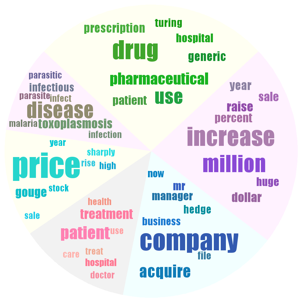
Figure 2: Topic Cloud of the pharmaceutical company acquisition news.

As shown in Figure 2, words in obtained topics were generally coherent, although the topics were only derived from a single document. The reason is that TopicVec takes advantage of the rich semantic information encoded in word embeddings, which were pretrained on a large corpus.

The topic coherence suggests that the derived topic embeddings were approximately the semantic centroids of the document. This capacity may aid applications such as document retrieval, where a “compressed representation” of the query document is helpful.

8 Conclusions and Future Work

In this paper, we proposed TopicVec, a generative model combining word embedding and LDA, with the aim of exploiting the word collocation patterns both at the level of the local context and the global document. Experiments show that TopicVec can learn high-quality document representations, even given only one document.

In our classification tasks we only explored the use of topic proportions of a document as its representation. However, jointly representing a document by topic proportions and topic embeddings would be more accurate. Efficient algorithms for this task have been proposed [Kusner et al., 2015].

Our method has potential applications in various scenarios, such as document retrieval, classification, clustering and summarization.

Acknowlegement

We thank Xiuchao Sui and Linmei Hu for their help and support. We thank the anonymous mentor for the careful proofreading. This research is funded by the National Research Foundation, Prime Minister’s Office, Singapore under its IDM Futures Funding Initiative and IRC@SG Funding Initiative administered by IDMPO. Part of the work was conceived when Shaohua Li was visiting Tsinghua. Jun Zhu is supported by National NSF of China (No. 61322308) and the Youngth Top-notch Talent Support Program.

Appendix A Derivation of $\mathcal{L}(q,\boldsymbol{T})$

The variational distribution is defined as:

$$q(\boldsymbol{Z},\boldsymbol{\phi};\boldsymbol{\pi},\boldsymbol{\theta})=q(\boldsymbol{\phi};\boldsymbol{\theta})q(\boldsymbol{Z};\boldsymbol{\pi})$$

$$= \prod_{i=1}^{M}\left\{\textrm{Dir}(\boldsymbol{\phi}_{i};\boldsymbol{\theta}_{i})\prod_{j=1}^{L_{i}}\textrm{Cat}(z_{ij};\boldsymbol{\pi}_{ij})\right\}.$$ (17)

Taking the logarithm of both sides of (17), we obtain

$$\log q(\boldsymbol{Z},\boldsymbol{\phi};\boldsymbol{\pi},\boldsymbol{\theta})$$

$$= \sum_{i=1}^{M}\Biggl{\{}\log\Gamma(\theta_{i0})-\sum_{k=1}^{K}\log\Gamma(\theta_{ik})$$

$$+\sum_{k=1}^{K}(\theta_{ik}-1)\log\phi_{ik}+\sum_{j,k=1}^{L_{i},K}\delta(z_{ij}=k)\log\pi_{ij}^{k}\Biggr{\}},$$

where $\theta_{i0}=\sum_{k=1}^{K}\theta_{ik}$, $\pi_{ij}^{k}$ is the $k$-th component of $\boldsymbol{\pi}_{ij}$.

Let $\psi(\cdot)$ denote the digamma function: $\psi(x)=\frac{d}{dx}\ln{\Gamma(x)}=\frac{\Gamma^{\prime}(x)}{\Gamma(x)}.$ It follows that

$$\mathcal{H}(q)$$

$$= -E_{q}[\log q(\boldsymbol{Z},\boldsymbol{\phi};\boldsymbol{\pi},\boldsymbol{\theta})]$$

$$= \sum_{i=1}^{M}\Biggl{\{}\sum_{k=1}^{K}\log\Gamma(\theta_{ik})-\log\Gamma(\theta_{i0})-\sum_{k=1}^{K}(\theta_{ik}-1)\psi(\theta_{ik})$$

$$+(\theta_{i0}-K)\psi(\theta_{i0})-\sum_{j,k=1}^{L_{i},K}\pi_{ij}^{k}\log\pi_{ij}^{k}\Biggr{\}}.$$ (18)

Plugging $q$ into $\mathcal{L}(q,\boldsymbol{T})$, we have

$$\mathcal{L}(q,\boldsymbol{T})$$

$$= \mathcal{H}(q)+E_{q}\left[\log p(\boldsymbol{Z},\boldsymbol{\phi}|\boldsymbol{T})\right]$$

$$= \mathcal{H}(q)+C_{0}-\log\mathcal{Z}(\boldsymbol{H},\boldsymbol{\mu})-\|\boldsymbol{A}\|_{f(\boldsymbol{H})}^{2}-\sum_{i=1}^{W}\mu_{i}\|\boldsymbol{v}_{s_{i}}\|^{2}$$

$$+\sum_{i=1}^{M}\bBigg@{3}\{\sum_{k=1}^{K}\left(E_{q(\boldsymbol{Z}_{i}|\boldsymbol{\pi}_{i})}[m_{ik}]+\alpha_{k}-1\right)\cdot E_{q(\phi_{ik}|\boldsymbol{\theta}_{i})}[\log\phi_{ik}$$

$$+\sum_{j=1}^{L_{i}}\Bigg{(}\boldsymbol{v}_{w_{ij}}^{\operatorname*{\scriptscriptstyle\top}}\Bigl{(}\sum_{k=j-c}^{j-1}\boldsymbol{v}_{w_{ik}}+E_{q(z_{ij}|\boldsymbol{\pi}_{ij})}[\boldsymbol{t}_{z_{ij}}]\Bigr{)}+\sum_{k=j-c}^{j-1}a_{w_{ik}w_{ij}}+E_{q(z_{ij}|\boldsymbol{\pi}_{ij})}[r_{i,z_{ij}}]\Bigg{)}\bBigg@{3}\}$$

$$= C_{1}+\mathcal{H}(q)+\sum_{i=1}^{M}\Biggl{\{}\sum_{k=1}^{K}\Bigl{(}\sum_{j=1}^{L_{i}}\pi_{ij}^{k}+\alpha_{k}-1\Bigr{)}\Bigl{(}\psi(\theta_{ik})-\psi(\theta_{i0})\Bigr{)}+\sum_{j=1}^{L_{i}}\Bigl{(}\boldsymbol{v}_{w_{ij}}^{\operatorname*{\scriptscriptstyle\top}}\boldsymbol{T}_{i}\boldsymbol{\pi}_{ij}+\boldsymbol{r}_{i}^{\operatorname*{\scriptscriptstyle\top}}\boldsymbol{\pi}_{ij}\Bigr{)}\Biggr{\}}$$

$$= C_{1}+\mathcal{H}(q)+\sum_{i=1}^{M}\Biggl{\{}\sum_{k=1}^{K}\Bigl{(}\sum_{j=1}^{L_{i}}\pi_{ij}^{k}+\alpha_{k}-1\Bigr{)}\Bigl{(}\psi(\theta_{ik})-\psi(\theta_{i0})\Bigr{)}$$

$$+\textrm{Tr}(\boldsymbol{T}_{i}^{\operatorname*{\scriptscriptstyle\top}}\sum_{j=1}^{L_{i}}\boldsymbol{v}_{w_{ij}}\boldsymbol{\pi}_{ij}^{\operatorname*{\scriptscriptstyle\top}})+\boldsymbol{r}_{i}^{\operatorname*{\scriptscriptstyle\top}}\sum_{j=1}^{L_{i}}\boldsymbol{\pi}_{ij}\Biggr{\}},$$ (19)

Appendix B Derivation of the E-Step

The learning objective is:

$$\mathcal{L}(q,\boldsymbol{T})$$

$$= \sum_{i=1}^{M}\Biggl{\{}\sum_{k=1}^{K}\Bigl{(}\sum_{j=1}^{L_{i}}\pi_{ij}^{k}+\alpha_{k}-1\Bigr{)}\Bigl{(}\psi(\theta_{ik})-\psi(\theta_{i0})\Bigr{)}$$

$$+\textrm{Tr}(\boldsymbol{T}_{i}^{\operatorname*{\scriptscriptstyle\top}}\sum_{j=1}^{L_{i}}\boldsymbol{v}_{w_{ij}}\boldsymbol{\pi}_{ij}^{\operatorname*{\scriptscriptstyle\top}})+\boldsymbol{r}_{i}^{\operatorname*{\scriptscriptstyle\top}}\sum_{j=1}^{L_{i}}\boldsymbol{\pi}_{ij}\Biggr{\}}+\mathcal{H}(q)+C_{1},$$ (20)

(20) can be expressed as

$$\mathcal{L}(q,\boldsymbol{T}^{(l-1)})$$

$$= \sum_{i=1}^{M}\Biggl{\{}\sum_{k=1}^{K}\log\Gamma(\theta_{ik})-\log\Gamma(\theta_{i0})-\sum_{k=1}^{K}(\theta_{ik}-1)\psi(\theta_{ik})+(\theta_{i0}-K)\psi(\theta_{i0})-\sum_{j,k=1}^{L_{i},K}\pi_{ij}^{k}\log\pi_{ij}^{k}$$

$$+\sum_{k=1}^{K}\Bigl{(}\sum_{j=1}^{L_{i}}\pi_{ij}^{k}+\alpha_{k}-1\Bigr{)}\Bigl{(}\psi(\theta_{ik})-\psi(\theta_{i0})\Bigr{)}+\sum_{j=1}^{L_{i}}\Bigl{(}\boldsymbol{v}_{w_{ij}}^{\operatorname*{\scriptscriptstyle\top}}\boldsymbol{T}_{i}\boldsymbol{\pi}_{ij}+\boldsymbol{r}_{i}^{\operatorname*{\scriptscriptstyle\top}}\boldsymbol{\pi}_{ij}\Bigr{)}\Biggr{\}}+C_{1}.$$ (21)

We first maximize (21) w.r.t. $\pi_{ij}^{k}$, the probability that the $j$-th word in the $i$-th document takes the $k$-th latent topic. Note that this optimization is subject to the normalization constraint that $\sum_{k=1}^{K}\pi_{ij}^{k}=1$.

We isolate terms containing $\boldsymbol{\pi}_{ij}$, and form a Lagrange function by incorporating the normalization constraint:

$$\Lambda(\boldsymbol{\pi}_{ij})=-\sum_{k=1}^{K}\pi_{ij}^{k}\log\pi_{ij}^{k}+\sum_{k=1}^{K}\Bigl{(}\psi(\theta_{ik})-\psi(\theta_{i0})\Bigr{)}\pi_{ij}^{k}+\boldsymbol{v}_{w_{ij}}^{\operatorname*{\scriptscriptstyle\top}}\boldsymbol{T}_{i}\boldsymbol{\pi}_{ij}+\boldsymbol{r}_{i}^{\operatorname*{\scriptscriptstyle\top}}\boldsymbol{\pi}_{ij}+\lambda_{ij}(\sum_{k=1}^{K}\pi_{ij}^{k}-1).$$ (22)

Taking the derivative w.r.t. $\pi_{ij}^{k}$, we obtain

$$\frac{\partial\Lambda(\boldsymbol{\pi}_{ij})}{\partial\pi_{ij}^{k}}=-1-\log\pi_{ij}^{k}+\psi(\theta_{ik})-\psi(\theta_{i0})+\boldsymbol{v}_{w_{ij}}^{\operatorname*{\scriptscriptstyle\top}}\boldsymbol{t}_{ik}+r_{ik}+\lambda_{ij}.$$ (23)

Setting this derivative to $0$ yields the maximizing value of $\pi_{ij}^{k}$:

$$\pi_{ij}^{k}\propto\exp\{\psi(\theta_{ik})+\boldsymbol{v}_{w_{ij}}^{\operatorname*{\scriptscriptstyle\top}}\boldsymbol{t}_{ik}+r_{ik}\}.$$ (24)

Next, we maximize (21) w.r.t. $\theta_{ik}$, the $k$-th component of the posterior Dirichlet parameter:

$$\frac{\partial\mathcal{L}(q,\boldsymbol{T}^{(l-1)})}{\partial\theta_{ik}}$$

$$= \frac{\partial}{\partial\theta_{ik}}\biggl{\{}\log\Gamma(\theta_{ik})-\log\Gamma(\theta_{i0})+\Bigl{(}\sum_{j=1}^{L_{i}}\pi_{ij}^{k}+\alpha_{k}-\theta_{ik}\Bigr{)}\psi(\theta_{ik})-\Bigl{(}L_{i}+\sum_{k}\alpha_{k}-\theta_{i0}\Bigr{)}\psi(\theta_{i0})\biggr{\}}$$

$$= \Bigl{(}\sum_{j=1}^{L_{i}}\pi_{ij}^{k}+\alpha_{k}-\theta_{ik}\Bigr{)}\psi^{\prime}(\theta_{ik})-\Bigl{(}L_{i}+\sum_{k}\alpha_{k}-\theta_{i0}\Bigr{)}\psi^{\prime}(\theta_{i0}),$$ (25)

where $\psi^{\prime}(\cdot)$ is the derivative of the digamma function $\psi(\cdot)$, commonly referred to as the trigamma function.

Setting (25) to $0$ yields a maximum at

$$\theta_{ik}=\sum_{j=1}^{L_{i}}\pi_{ij}^{k}+\alpha_{k}.$$ (26)

Note this solution depends on the values of $\pi_{ij}^{k}$, which in turn depends on $\theta_{ik}$ in (24). Then we have to alternate between (24) and (26) until convergence.

Appendix C Derivative of $\mathcal{L}(q^{(l)},\boldsymbol{T})$ w.r.t. $\boldsymbol{T}_{i}$:

$$\frac{\partial\mathcal{L}(q^{(l)},\boldsymbol{T})}{\partial\boldsymbol{T}_{i}}$$

$$= \frac{\partial\sum_{j=1}^{L_{i}}\left(\boldsymbol{v}_{w_{ij}}^{\operatorname*{\scriptscriptstyle\top}}\boldsymbol{T}_{i}\boldsymbol{\pi}_{ij}+\boldsymbol{\pi}_{ij}^{\operatorname*{\scriptscriptstyle\top}}\boldsymbol{r}_{i}\right)}{\partial\boldsymbol{T}_{i}}$$

$$= \frac{\partial}{\partial\boldsymbol{T}_{i}}\textrm{Tr}(\boldsymbol{T}_{i}\sum_{j=1}^{L_{i}}\boldsymbol{\pi}_{ij}\boldsymbol{v}_{w_{ij}}^{\operatorname*{\scriptscriptstyle\top}})+(\sum_{j=1}^{L_{i}}\boldsymbol{\pi}_{ij})^{\operatorname*{\scriptscriptstyle\top}}\frac{\partial\boldsymbol{r}_{i}}{\partial\boldsymbol{T}_{i}}$$

$$= \sum_{j=1}^{L_{i}}\boldsymbol{v}_{w_{ij}}\boldsymbol{\pi}_{ij}^{\operatorname*{\scriptscriptstyle\top}}+(\sum_{j=1}^{L_{i}}\boldsymbol{\pi}_{ij})^{\operatorname*{\scriptscriptstyle\top}}\frac{\partial\boldsymbol{r}_{i}}{\partial\boldsymbol{T}_{i}}$$

$$= \sum_{j=1}^{L_{i}}\boldsymbol{v}_{w_{ij}}\boldsymbol{\pi}_{ij}^{\operatorname*{\scriptscriptstyle\top}}+\sum_{k=1}^{K}\bar{m}_{ik}\frac{\partial r_{ik}}{\partial\boldsymbol{T}_{i}},$$ (27)

where $\bar{m}_{ik}=\sum_{j=1}^{L_{i}}\pi_{ij}^{k}=E[m_{ik}]$, the sum of the variational probabilities of each word being assigned to the $k$-th topic in the $i$-th document.

References

- [Bengio et al., 2003] Yoshua Bengio, Réjean Ducharme, Pascal Vincent, and Christian Jauvin. 2003. A neural probabilistic language model. Journal of Machine Learning Research, pages 1137–1155.
- [Blei et al., 2003] David M Blei, Andrew Y Ng, and Michael I Jordan. 2003. Latent dirichlet allocation. the Journal of machine Learning research, 3:993–1022.
- [Das et al., 2015] Rajarshi Das, Manzil Zaheer, and Chris Dyer. 2015. Gaussian LDA for topic models with word embeddings. In Proceedings of the 53rd Annual Meeting of the Association for Computational Linguistics and the 7th International Joint Conference on Natural Language Processing (Volume 1: Long Papers), pages 795–804, Beijing, China, July. Association for Computational Linguistics.
- [Hinton and Salakhutdinov, 2009] Geoffrey E Hinton and Ruslan R Salakhutdinov. 2009. Replicated softmax: an undirected topic model. In Advances in neural information processing systems, pages 1607–1614.
- [Huang et al., 2012] Eric H Huang, Richard Socher, Christopher D Manning, and Andrew Y Ng. 2012. Improving word representations via global context and multiple word prototypes. In Proceedings of the 50th Annual Meeting of the Association for Computational Linguistics: Long Papers-Volume 1, pages 873–882. Association for Computational Linguistics.
- [Kusner et al., 2015] Matt Kusner, Yu Sun, Nicholas Kolkin, and Kilian Q. Weinberger. 2015. From word embeddings to document distances. In David Blei and Francis Bach, editors, Proceedings of the 32nd International Conference on Machine Learning (ICML-15), pages 957–966. JMLR Workshop and Conference Proceedings.
- [Larochelle and Lauly, 2012] Hugo Larochelle and Stanislas Lauly. 2012. A neural autoregressive topic model. In Advances in Neural Information Processing Systems, pages 2708–2716.
- [Le and Mikolov, 2014] Quoc Le and Tomas Mikolov. 2014. Distributed representations of sentences and documents. In Proceedings of the 31st International Conference on Machine Learning (ICML-14), pages 1188–1196.
- [Levy et al., 2015] Omer Levy, Yoav Goldberg, and Ido Dagan. 2015. Improving distributional similarity with lessons learned from word embeddings. Transactions of the Association for Computational Linguistics, 3:211–225.
- [Li et al., 2015] Shaohua Li, Jun Zhu, and Chunyan Miao. 2015. A generative word embedding model and its low rank positive semidefinite solution. In Proceedings of the 2015 Conference on Empirical Methods in Natural Language Processing, pages 1599–1609, Lisbon, Portugal, September. Association for Computational Linguistics.
- [Li et al., 2016] Shaohua Li, Jun Zhu, and Chunyan Miao. 2016. PSDVec: a toolbox for incremental and scalable word embedding. To appear in Neurocomputing.
- [Liu et al., 2015] Yang Liu, Zhiyuan Liu, Tat-Seng Chua, and Maosong Sun. 2015. Topical word embeddings. In AAAI, pages 2418–2424.
- [Lu et al., 2011] Yue Lu, Qiaozhu Mei, and ChengXiang Zhai. 2011. Investigating task performance of probabilistic topic models: an empirical study of PLSA and LDA. Information Retrieval, 14(2):178–203.
- [McAuliffe and Blei, 2008] Jon D McAuliffe and David M Blei. 2008. Supervised topic models. In Advances in neural information processing systems, pages 121–128.
- [Mikolov et al., 2013] Tomas Mikolov, Ilya Sutskever, Kai Chen, Greg S Corrado, and Jeff Dean. 2013. Distributed representations of words and phrases and their compositionality. In Proceedings of NIPS 2013, pages 3111–3119.
- [Nguyen et al., 2015] Dat Quoc Nguyen, Richard Billingsley, Lan Du, and Mark Johnson. 2015. Improving topic models with latent feature word representations. Transactions of the Association for Computational Linguistics, 3:299–313.
- [Pennington et al., 2014] Jeffrey Pennington, Richard Socher, and Christopher D Manning. 2014. GloVe: Global vectors for word representation. Proceedings of the Empiricial Methods in Natural Language Processing (EMNLP 2014), 12.