Analytical investigation of the decrease in the size of the habitable zone due to limited CO₂ outgassing rate

Abstract

The habitable zone concept is important because it focuses the scientific search for extraterrestrial life and aids the planning of future telescopes. Recent work has shown that planets near the outer edge of the habitable zone might not actually be able to stay warm and habitable if CO₂ outgassing rates are not large enough to maintain high CO₂ partial pressures against removal by silicate weathering. In this paper I use simple equations for the climate and CO₂ budget of a planet in the habitable zone that can capture the qualitative behavior of the system. With these equations I derive an analytical formula for an effective outer edge of the habitable zone, including limitations imposed by the CO₂ outgassing rate. I then show that climate cycles between a Snowball state and a warm climate are only possible beyond this limit if the weathering rate in the Snowball climate is smaller than the CO₂ outgassing rate (otherwise stable Snowball states result). I derive an analytical solution for the climate cycles including a formula for their period in this limit. This work allows us to explore the qualitative effects of weathering processes on the effective outer edge of the habitable zone, which is important because weathering parameterizations are uncertain.

1 Introduction

The habitable zone is defined as the region around a star where a planet with CO₂ and H₂O as its main greenhouse gases can support liquid water at its surface (Kasting et al., 1993). The habitable zone is relatively wide because of the silicate-weathering feedback (Walker et al., 1981). Silicate-weathering is a geological process that removes CO₂ from the atmosphere and a negative (stabilizing) feedback is possible because this process is believed to run faster at higher temperatures and higher CO₂ partial pressures (Pierrehumbert, 2010). The inner edge of the habitable zone is set by the moist or runaway greenhouse (Kasting, 1988; Nakajima et al., 1992; Goldblatt & Watson, 2012), which should not be influenced by the details of the silicate-weathering feedback since the CO₂ should have been drawn down to low levels when they occur. On the other hand, calculations of the outer edge of the habitable zone generally assume that the silicate-weathering feedback can maintain CO₂ at arbitrarily high levels. The outer edge is then marked by some threshold where adding CO₂ to the atmosphere no longer provides additional warming, for example if additional CO₂ increases Rayleigh scattering more than it increases greenhouse warming (Kasting et al., 1993; Kopparapu et al., 2013). This picture essentially considers the asymptotic limit of unlimited CO₂ outgassing capacity.

More recently it has been recognized that for finite CO₂ outgassing rates the maximum CO₂ that a planet can achieve may be lower than the CO₂ needed to keep that planet habitable at the outer edge of the habitable zone (Tajika, 2007; Kadoya & Tajika, 2014). This leads to what I will call the “effective outer edge of the habitable zone,” which will depend on the CO₂ outgassing rate and the functioning of silicate weathering on the planet. Beyond the effective outer edge of the habitable zone, a planet may experience cycles (Menou, 2015; Haqq-Misra et al., 2016) between a globally frozen, Snowball Earth climate (Kirschvink, 1992; Hoffman et al., 1998) and a habitable climate. Understanding and constraining the effective outer edge of the habitable zone is critical because it determines our estimate of the fraction of stars that host an Earth-like planet (Petigura et al., 2013; Kopparapu, 2013), which is essential for planning future telescopes that would observe such planets.

The purpose of this paper is to investigate what determines the position of the effective outer edge of the habitable zone and what happens beyond the effective outer edge. The behavior of a planet in this regime is largely determined by its uncertain silicate-weathering behavior. Instead of viewing this an an obstacle, I will exploit it to make progress on the problem. The importance and uncertainty of weathering justifies the use of a simple climate model since the errors associated with making the grave assumptions that such a model entails pale in comparison to the uncertainty in weathering. It also allows me to use a relatively simple weathering parameterization that captures the expected qualitative behavior. I will use the simplifying assumptions to derive useful formulae. This will allow us to understand issues such as which processes determine whether the effective outer edge of the habitable zone is inside the traditional outer edge of the habitable zone and how much the parameters associated with these processes would need to be changed from our best estimates of their values to change the qualitative behavior of the system. Moreover, I am able to determine the conditions for climate cycles to occur beyond the effective outer edge of the habitable zone, an analytical solution for these cycles, and a formula for the period of the cycles. Using more complicated climate and weathering models will alter quantitative results, but is unlikely to alter the qualitative dependencies on parameters that my formulae give. This work therefore complements recent work by Menou (2015) and Haqq-Misra et al. (2016), who used more complicated radiative and climate models, but only explored a few values of weathering parameters.

I will neglect sophisticated radiative (Kopparapu, 2013; Goldblatt et al., 2013) and 3D calculations (Leconte et al., 2013b, a; Yang et al., 2013, 2014; Wolf & Toon, 2014, 2015) and consider the following linearized, zero-dimensional model of planetary climate, similar to that used by (Abbot et al., 2012):

$$C\frac{dT}{dt}=\frac{S}{4}(1-\alpha(T))-\frac{S_{0}}{4}(1-\alpha_{o})-a(T-T_{0})+b\log\left(\frac{P}{P_{0}}\right),$$ (1)

where $a$ and $b$ are constants, $T$ is the global mean temperature, $T_{0}$ is the temperature of the reference state, $P$ is the atmospheric partial pressure of CO₂, $P_{0}$ is the atmospheric partial pressure of CO₂ in the reference state, $S$ is the stellar flux, $S_{0}$ is the stellar flux in the reference state, $C$ is the heat capacity in units of J m^-2 ∘C^-1, $\alpha(T)$ is the temperature-dependent planetary albedo (reflectivity), and $\alpha_{0}$ is the albedo of the reference state. Table 1 contains a list model parameters and their standard values. The values I use here are drawn from Abbot et al. (2012), Menou (2015), and Haqq-Misra et al. (2016), but it is important to emphasize that the arguments in this paper do not depend on the exact values chosen.

I will let the albedo be specified by

$$\alpha(T)=\begin{cases}\alpha_{w},\ T\geq T_{i},\\ \alpha_{c},\ T<T_{i},\end{cases}$$ (2)

where $\alpha_{w}$ is the albedo of the warm climate state; $\alpha_{c}$ is the albedo of the cold and icy, “Snowball” climate state; and $T_{i}$ is the temperature at which the planet transitions between the two climate states. Equation (2) assumes a step-wise transition in albedo, which neglects the effects of spatial resolution (Yang et al., 2012a, b, c; Voigt et al., 2011; Voigt & Abbot, 2012). Nevertheless, it allows us to make easier analytical progress and does not alter the qualitative behavior of the system unless multiple Snowball-like climate states possible (Abbot et al., 2011; Rose, 2015), which is a possibility we will not consider here. As we will see below, introducing a smoothed albedo transition only introduces a repulsing fixed point in some situations that the climate could not exist stably in. Finally, if we assume that the reference climate state is warm, then $\alpha_{0}=\alpha_{w}$.

The partial pressure of CO₂ is determined by outgassing and weathering

$$\frac{dP}{dt}=V-W_{0}e^{k(T-T_{0})}\left(\frac{P}{P_{0}}\right)^{\beta},$$ (3)

where $V$ is the CO₂ outgassing rate, $W_{0}$ is the rate of removal of CO₂ from the atmosphere by silicate weathering in the reference climate state, $k$ is a rate constant for the increase in weathering with temperature, and $\beta$ is an exponent that determines how strongly weathering depends on atmospheric CO₂ partial pressure. West et al. (2005) used an analysis of river catchments to estimate that $k=0.11\pm 0.04$ ^∘C^-1 (1-$\sigma$ error). Based on that study, the plausible range for $k$ is roughly 0–0.2. I will use a standard value of $k$=0.1 and vary $k$ over this range. $\beta$ could be zero if land plants concentrate CO₂ in the soil at the same level regardless of the atmospheric CO₂ concentration (Pierrehumbert, 2010), and theoretical arguments suggest $\beta$ has a maximum of 1 (Berner, 1994). I will use a standard value of $\beta$=0.5 (Berner, 1994; Pierrehumbert, 2010; Abbot et al., 2012; Menou, 2015; Haqq-Misra et al., 2016), but consider variations within the plausible range. Depressurization caused by glacial unloading can cause temporary increases in the CO₂ outgassing rate (Huybers & Langmuir, 2009). I neglect this affect and take the CO₂ outgassing rate to be independent climate state here, which is appropriate for longterm average behavior. Note also that in section 4 we will consider $W_{0}$=0 when $T<T_{i}$.

For the purposes of this paper I am assuming that weathering follows a similar parameterization on land and at the seafloor, but it should be understood that the weathering behavior of an ocean planet would likely be quite different from that of a planet with an Earth-like land fraction (Abbot et al., 2012). The weathering parameterization in Equation (3) is similar to that used by other authors (Berner, 1994, 2004; Pierrehumbert, 2010; Abbot et al., 2012; Menou, 2015; Haqq-Misra et al., 2016), but I have dropped the relatively weak dependence on temperature that is often included to represent changes in precipitation with temperature. The qualitative behavior of weathering as a function of temperature is captured by Equation (3) without this additional complication. Given the ad hoc nature of all weathering parameterizations, it is reasonable to choose the simplest parameterization that gives the expected qualitative behavior of weathering processes given the objectives of this paper.

Equations (1)-(3) define the system. The plan for analyzing them is as follows. First we will consider the warm (habitable) state (section 2). I will set the albedo (Equation (2)) to its warm state value, set the time derivatives in Equations (1) and (3) to zero, and solve the system for conditions when the temperature is high enough for the warm state to exist. This will allow us to put bounds on the existence of the warm state, that is, define an effective outer edge of the habitable zone that may be more restrictive than the traditional outer edge. Next I will find nullclines of the system defined by Equations (1) and (3) (that is, lines where the time derivatives equal zero), find their intersections (fixed points, or solutions of the system), and determine the stability of these fixed points. Physically, this will reveal that if Equation (3) is followed as is, enough weathering occurs that the system settles into a stable Snowball state when the warm climate state ceases to exist, rather than into climate cycles between Snowball and warm conditions. I will then show that climate cycles do occur if we set weathering to zero in the Snowball state in Equation (3) (section 4). I will find analytical solutions for the components of these cycles and derive an analytical formula for their period that can predict well results from the more intricate model of (Menou, 2015). I will then discuss these results in section 5 and conclude in section 6.

Table 1: A list of the model parameters, their descriptions, and the standard values I use for them. The parameter values in this table are taken from Abbot et al. (2012), Menou (2015), and Haqq-Misra et al. (2016). Note that, following Haqq-Misra et al. (2016), I use a value of $W_{0}$ ten times higher than Menou (2015). I perform sensitivity analyses where I vary $k$ and $\beta$.

Parameter	Description	Standard Value
$S_{0}$	reference state stellar flux	1365.0 W m-2
$S$	stellar flux	variable
$T_{0}$	reference state temperature	15.0∘C
$P_{0}$	reference state partial pressure CO2	3$\times 10^{-4}$ bars
$a$	slope of planetary infrared emission with temperature	2.0 W m-2 ∘C-1
$b$	slope of planetary infrared emission with logarithm of CO2	10.0 W m-2
$\alpha_{0}$	reference state albedo	0.3
$\alpha_{w}$	warm state albedo	0.3
$\alpha_{c}$	cold state albedo	0.6
$T_{i}$	albedo transition temperature	-10∘C
$C$	planetary heat capacity	2$\times 10^{8}$ J m-2 ∘C-1
$V$	CO2 outgassing rate	variable
$W_{0}$	reference state CO2 weathering rate	70 bars Gyr-1
$k$	weathering-temperature rate constant	0.1 ∘C-1
$\beta$	weathering-CO2 power law exponent	0.5

2 Conditions on the existence of a habitable climate state

In this section we will consider the conditions that allow the carbon cycle to maintain a planet in the warm climate state, which is necessary for the planet to be considered habitable in the traditional sense. This requires a steady-state solution, so we can set the time derivatives in Equations (1) and (3) to zero. We can solve this system to find

$$T_{w}-T_{0}=\frac{b\log\left(\frac{V}{W_{0}}\right)+\frac{\beta}{4}(S-S_{0})(1-\alpha_{w})}{kb+a\beta},$$ (4)

where $T_{w}$ is the warm state temperature. We could rewrite Equation (4) in non-dimensional form, but I will leave it, and subsequent equations, in dimensionful form to make them more accessible physically. From Equation (4) we can see that increasing the CO₂ outgassing rate logarithmically increases the warm state temperature, and that increased outgassing warms the warm state more if the climate is more sensitive to CO₂ (higher $b$), provided $\beta\neq 0$. We can also see that the influence of stellar flux on the warm state temperature depends on $\beta$, the weathering-CO₂ power-law exponent. If $\beta=0$, then changing the stellar flux has no effect on the warm state temperature as long as the stellar flux is high enough that $T_{w}\geq T_{i}$, so that the warm state can exist. Instead, the warm state temperature is determined by the outgassing rate. As $\beta$ increases, the warm climate state becomes increasingly sensitive to changes in stellar flux.

We can solve for the warm state CO₂ partial pressure ($P_{w}$) as follows

$$\log\left(\frac{P_{w}}{P_{0}}\right)=\frac{a\log\left(\frac{V}{W_{0}}\right)+\frac{k}{4}(S_{0}-S)(1-\alpha_{w})}{kb+a\beta}.$$ (5)

The warm state CO₂ partial pressure has a power law dependence on the CO₂ outgassing rate. The exponent depends most strongly on $a$, which determines the increase in outgoing longwave radiation with temperature. The more that increasing the warm state temperature by a given amount increases longwave cooling, the higher the warm state CO₂ must be to maintain that temperature at a given CO₂ outgassing rate. As expected, the warm state CO₂ partial pressure is exponentially lower if the stellar flux is higher. This effect is mediated mainly by $k$, the parameter that determines the increase in weathering with temperature. If $k$ is higher, then a given warming from an increase in stellar flux causes the weathering to increase more, and draws down the CO₂ more.

Using Equation (4), we can solve for the coldest possible warm state by setting $T_{w}=T_{i}$. This is a very important condition because habitability would be lost if anything were to cool the climate when it is in the coldest possible warm state. We can solve for the stellar flux at which the coldest possible warm state exists ($S^{\ast}$), which we can think as the effective outer edge of the habitable zone, as follows

$$S^{\ast}=S_{0}-\left(\frac{4}{1-\alpha_{w}}\right)\left(\frac{b}{\beta}\log\left(\frac{V}{W_{0}}\right)+k(T_{0}-T_{i})\left(\frac{b}{\beta}+\frac{a}{k}\right)\right).$$ (6)

A lower value of $S^{\ast}$ means that the stellar flux must be decreased more to reach the coldest possible warm state, which means that the warm climate state exists in more of the habitable zone. The ideal situation for habitability is when $S^{\ast}$ is decreased enough that it is smaller than the outer edge of the habitable zone, the point at which some other process, such as Rayleigh scattering, prevents CO₂ from warming the planetary surface. If this is the case then the silicate-weathering feedback can keep a planet habitable throughout the entire habitable zone.

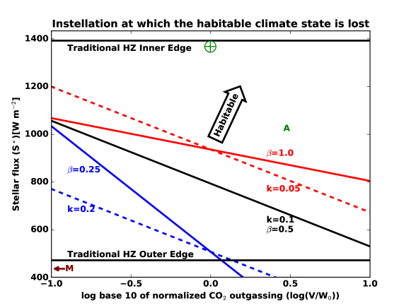
Figure 1: The stellar flux at which the habitable climate state is lost (the effective outer edge of the habitable zone) as a function of the logarithm of the normalized CO₂ outgassing (black line for standard parameters). The different curves show the behavior for different values of the weathering-CO₂ power law exponent ($\beta$, solid red and blue lines) and the weathering-temperature rate constant ($k$, dashed red and blue lines), both of which are relatively unconstrained. Red lines indicate changes to parameters that restrict the region where the habitable climate state can exist and blue lines indicate changes to parameters that expand this region. The traditional inner and outer edges of the habitable zone from Kopparapu et al. (2013) are at the top and bottom of this plot. The symbol $\bigoplus$ represents modern Earth, the “A” represents Earth 3.8 Gyr ago assuming 75% modern Earth’s stellar flux (i.e., insolation, Gough, 1981) and a CO₂ outgassing rate of three times modern, and the “M” represents Mars 3.8 Gyr ago assuming a CO₂ outgassing rate of 1 bar Gyr^-1 (Grott et al., 2011), which would plot to the left of the minimum CO₂ outgassing rate shown here. The CO₂ outgassing rate on early Earth is not well-constrained, but probably was higher than modern (Dasgupta, 2013).

The first thing we can note from Equation (6) is that if the albedo of the warm state is smaller, the effective outer edge of the habitable zone will be further out. Since absorption of stellar flux by atmospheric water vapor should be larger for planets orbiting smaller, redder stars (Kasting et al., 1993), the effective outer edge of the habitable zone is less likely to restrict the traditional habitable zone for M-stars than for G-stars and more likely for F-stars, which is consistent with what has been recently found by Haqq-Misra et al. (2016). Equation (6) also tells us that the effective outer edge of the habitable zone depends only logarithmically on the CO₂ outgassing rate. This is important because it tells us that large changes in the CO₂ outgassing rate are necessary to significantly change the effective outer edge. For example, increasing the CO₂ outgassing rate by a factor of ten only decreases the effective outer edge from 794 W m^-2 to 530 W m^-2, for our standard parameters (Figure 1). Changing the weathering parameters can have a much larger effect, which we can investigate by doing a sensitivity analysis in which we vary them. For example, either increasing the weathering-temperature rate constant ($k$) by a factor of two or decreasing the weathering-CO₂ power law exponent ($\beta$) by a factor of two causes a similar reduction in the effective outer edge as increasing the CO₂ outgassing by a factor of ten (Figure 1).

Changing $k$ and changing $\beta$ have qualitatively different effects on the response of $S^{\ast}$ to changes in the CO₂ outgassing rate (Figure 1). Decreasing $\beta$ increases the slope of $S^{\ast}$ as a function of $\log\left(\frac{V}{W_{0}}\right)$, which means that increasing the CO₂ outgassing rate by a given amount extends the effective habitable zone further (Equation (6)). This is because the temperature becomes more sensitive to the CO₂ outgassing rate when $\beta$ is smaller (Equation (4)). Alternatively, changing $k$ changes the offset of the $S^{\ast}$ versus $\log\left(\frac{V}{W_{0}}\right)$ line, but not the slope. A higher value of $k$ means that the temperature has to change less to cause the same change in weathering rate. This allows the stellar flux to be dropped to a lower value before the warm state temperature reaches the temperature at which the warm state is lost ($T_{w}=T_{i}$).

For reference I have plotted the estimated positions of modern Earth, Earth 3.8 Gyr ago, and Mars 3.8 Gyr on Figure 1. The simple model used here indicates that early and modern Earth are safely inside the effective outer edge of the habitable zone, whereas early Mars would have been beyond the effective outer edge of the habitable zone even if it were within the traditional habitable zone. This is consistent with the histories of the two planets if we assume that fluvial features on early Mars were episodic (Wordsworth et al., 2013; Halevy & Head III, 2014; Kite et al., 2015). That said, it should be understood that specific conclusions like these depend on details of weathering parameterizations, and the purpose of this paper is to expose the qualitative effects of weathering, rather than to try to answer detailed questions.

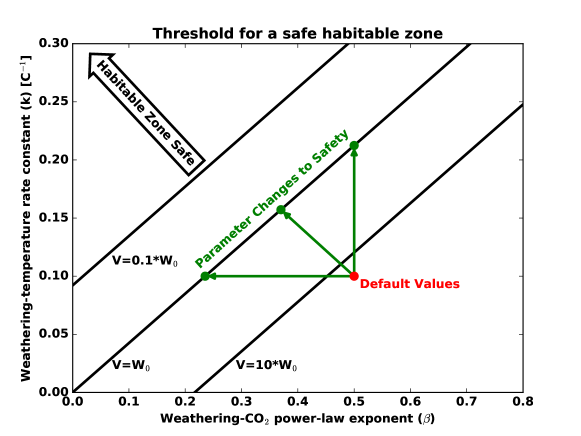
Figure 2: Lines of the weathering-temperature rate constant ($k$) as a function of the weathering-CO₂ power law exponent ($\beta$) at which the effective outer edge of the habitable zone equals the traditional outer edge. These lines are plotted for three different values of the CO₂ outgassing rate (0.1, 1, and 10 times modern Earth’s value). If the $k$ and $\beta$ combination is to the upper left of this plot relative to a given line, then CO₂ outgassing does not limit habitability and the full habitable zone is saved.

Another way we can think about this is to consider the set of weathering parameters that would make the effective outer edge of the habitable zone correspond to the traditional outer edge of the habitable zone. If we denote the traditional outer edge of the habitable zone as $S^{\ast}_{out}$, we can rewrite Equation (6) as

$$k=-\frac{\log\left(\frac{V}{W_{0}}\right)}{T_{0}-T_{i}}+\frac{\beta}{b}\left(\frac{\frac{1}{4}(S_{0}-S^{\ast}_{out})(1-\alpha_{w})}{T_{0}-T_{i}}-a\right).$$ (7)

Equation (7) represents a series of lines of $k$ as a function of $\beta$ for different values of the CO₂ outgassing rate. If $k$ is larger or $\beta$ is smaller than the line for a particular CO₂ outgassing rate, then the effective habitable zone is just as large as the traditional habitable zone for this CO₂ outgassing rate. Figure 2 shows three such curves for different CO₂ outgassing rates. For the default values of $k$ and $\beta$, some of the habitable zone would be lost even if the CO₂ outgassing rate were ten times higher than modern Earth’s ($\frac{V^{\ast}}{W_{0}}=16.6$ would be required for the effective outer edge to equal the traditional outer edge). However, relatively small changes to $k$, $\beta$, or some combination of the two can save the habitable zone even for modern Earth’s CO₂ outgassing rate (Figure 2). The parameters $k$ and $\beta$ are uncertain and may vary between planets, but the expressions in this section could be used for a probabilistic estimate of planetary habitability if appropriate priors are used for $k$ and $\beta$.

3 What happens when the habitable climate state ceases to exist

If the stellar flux or CO₂ outgassing rate is lowered enough that the warm climate state no longer exists, the planet enters a Snowball state and the albedo increases according to Equation (2). It is an open question how weathering would behave in a Snowball state. Menou (2015) assumed that weathering would go to zero due to lack of rain (liquid water), and we will consider this case in section 4. The possibility remains, however, that weathering could continue to occur under wet-based ice sheets or at the seafloor (Le Hir et al., 2008). For illustrative purposes, we will continue to use Equation (3) to characterize weathering in the Snowball state, but it should be understood that either subglacial or seafloor weathering could lead to different parameterizations. As we will see, however, the important point is that if some CO₂-dependent weathering can occur in the Snowball state, and it causes weathering to increase enough to balance CO₂ outgassing before the Snowball deglaciates, then it is possible for this state to be a stable solution of the system.

We can solve for the temperature tendency nullcline (the line on which $\frac{dT}{dt}$=0 in Equation (1)), which results in

$$\log\left(\frac{P}{P_{0}}\right)=\begin{cases}\frac{1}{b}\left(a(T-T_{0})+\frac{1}{4}S_{0}(1-\alpha_{w})-\frac{1}{4}S(1-\alpha_{w})\right),\ T\geq T_{i}\\ \frac{1}{b}\left(a(T-T_{0})+\frac{1}{4}S_{0}(1-\alpha_{w})-\frac{1}{4}S(1-\alpha_{c})\right),\ T<T_{i}.\end{cases}$$ (8)

Equation (8) describes two lines of $\log\left(\frac{P}{P_{0}}\right)$ as a function of $T-T_{0}$, each with a slope of $\frac{a}{b}$. The colder solution has a larger vertical offset. This is because more CO₂ would be required to keep the cold state at a given temperature than the warm state because the albedo is higher in the cold state (although they can never actually exist at the same temperature). Similarly, we solve for the CO₂ partial pressure tendency nullcline (the line on which $\frac{dP}{dt}$=0 in Equation (3)) to find

$$\log\left(\frac{P}{P_{0}}\right)=\frac{1}{\beta}\log\left(\frac{V}{W_{0}}\right)-\frac{k}{\beta}(T-T_{0}).$$ (9)

Equation (9) describes a line of $\log\left(\frac{P}{P_{0}}\right)$ as a function of $T-T_{0}$ with a slope of $-\frac{k}{\beta}$. Since the slope is negative, there will always be at least one intersection of the two nullclines, which will be a steady-state of the system. As the CO₂ outgassing rate ($V$) increases, the intercept of Equation (9) is increased and the solution becomes warmer. For high values of $V$ only the warm state is a steady state, and for low values only the cold state is a steady state. For intermediate values of $V$ it is possible to have both states to be a steady state of the system.

We already solved for the warm state temperature and CO₂ in Equations (4) and (5). We can now solve for the cold state temperature ($T_{c}$) and CO₂ ($P_{c}$) using the cold branch of Equation (8)

$$T_{c}-T_{0}=\frac{b\log\left(\frac{V}{W_{0}}\right)+\frac{\beta}{4}S(1-\alpha_{c})-\frac{\beta}{4}S_{0}(1-\alpha_{w})}{kb+a\beta},$$ (10)

$$\log\left(\frac{P_{c}}{P_{0}}\right)=\frac{a\log\left(\frac{V}{W_{0}}\right)+\frac{k}{4}S_{0}(1-\alpha_{w})-\frac{k}{4}S(1-\alpha_{c})}{kb+a\beta}.$$ (11)

The final point of interest is to determine the stability of the fixed points described by Equations (4), (5), (10), and (11). We can do this by evaluating the Jacobian ($J$) of the system at the fixed points

$$J=\begin{bmatrix}\frac{\partial}{\partial T}\frac{dT}{dt}&\frac{\partial}{\partial P}\frac{dT}{dt}\\ \frac{\partial}{\partial T}\frac{dP}{dt}&\frac{\partial}{\partial P}\frac{dP}{dt}\end{bmatrix}=\begin{bmatrix}-\frac{a}{C}&\frac{b}{CP}\\ -kW_{0}e^{k(T-T_{0})}\left(\frac{P}{P_{0}}\right)^{\beta}&-\frac{W_{0}}{P_{0}}\beta e^{k(T-T_{0})}\left(\frac{P}{P_{0}}\right)^{\beta-1}\end{bmatrix}.$$ (12)

For both the warm and cold states, the trace of the Jacobian ($\tau$) is less than zero and its determinant ($\Delta$) is greater than zero. This means that the warm and cold states are always attracting (Strogatz, 1994). $\tau^{2}-4\Delta$ is generally positive, which means that the fixed points will usually be stable nodes, although it is possible for them to be stable spirals for some parameter combinations.

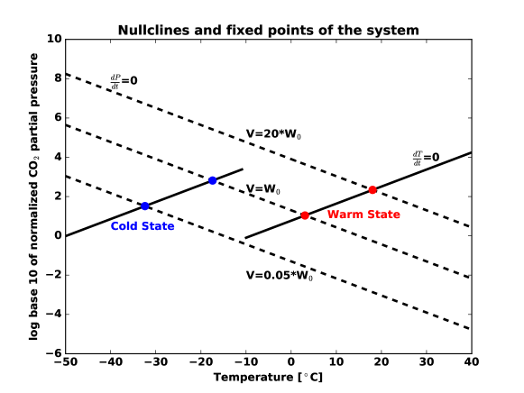
Figure 3: This plot shows nullclines of the system, where either the temperature tendency is zero ($\frac{dT}{dt}$=0, solid lines) or the CO₂ partial pressure tendency is zero ($\frac{dP}{dt}$=0, dashed lines). Three pressure partial pressure tendency nullclines are shown: for a CO₂ outgassing rate of 0.05, 1, and 20 times modern Earth’s. The intersections of these nullclines represent fixed points of the system, which are all attractors. Warm climate state fixed points are plotted in red and cold climate state fixed points are plotted in blue. For higher CO₂ outgassing rates only the warm state exists, for lower rates only the cold state exists, and at intermediate rates both the warm and cold climate states exist. The stellar flux is 80% of modern Earth’s in this figure.

I have plotted what we have learned about the nullclines and their intersections for a representative set of parameters in Figure 3. This plot shows how intersections of the nullclines lead to steady states, and how at least one intersection will always occur since the CO₂ partial pressure tendency nullcline has a negative slope and the two temperature tendency nullclines have a positive slope. Note that although the simplicity of the model we are considering constrains the nullclines to be linear, we would expect similar, but potentially nonlinear, behavior from a more complicated model. For example, if we used a more sophisticated radiative transfer model for the climate calculations (e.g., Kopparapu et al., 2013) it would lead to curvature in the temperature tendency nullclines, but no change in the topology of the system.

Because we have assumed a discontinous albedo transition (Equation (2)) stable fixed points appear and disappear in isolation in Figure 3. If we had instead assumed a smoothed albedo transition, for example smoothed with a hyperbolic tangent function, the two temperature tendency nullclines would smoothly join together. In this case, there would always be an unstable saddle fixed point between the two attracting fixed points representing the warm and Snowball climate states when both attracting states exist at the same CO₂ outgassing rate. If the CO₂ outgassing rate were changed sufficiently, the saddle fixed point would merge with either of the attracting fixed points in a saddle node bifurcation, rather than the attracting fixed point just disappearing as it does in the discontinous albedo system.

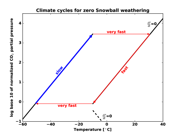
Figure 4: Plot of the climate cycles that occur when both (1) the CO₂ outgassing rate is too low to achieve a warm climate steady state and (2) the weathering rate is set to zero when the temperature is less than the Snowball transition temperature ($T<T_{i}$). This plot is similar to Figure 3, but the CO₂ partial pressure nullcline ends for $T<T_{i}$ because there is no way for the time derivative of the CO₂ partial pressure to be zero if the weathering rate is zero. There is no steady state and instead planetary climate experiences a limit cycle with four stages. Most of the time is spent with the planet in the Snowball state, where it warms very slowly as a result of CO₂ outgassing.

4 Climate cycles when the Snowball weathering is set to zero

Alternatively, we can consider the situation where the weathering rate is smaller than the CO₂ outgassing rate for temperatures less than the temperature at which the planet transitions between the two climate states ($T<T_{i}$). For simplicity, I will set the weathering rate to zero for $T<T_{i}$, following Menou (2015). In this case no Snowball steady state is possible because there is no weathering term to balance CO₂ outgassing when the planet is experiencing a Snowball (Equation (3)). Instead CO₂ simply accumulates in the Snowball state, warming it, until the temperature $T_{i}$ is reached. This causes the albedo to decrease (physically the ice melts) and the planet abruptly jumps into the warm climate state. If we assume that the CO₂ outgassing rate is low enough that no warm climate steady state exists, then the warm climate leads to the rapid removal of CO₂ by weathering until $T_{i}$ is again reached, then the climate abruptly jumps into the Snowball state, and the cycle repeats. Figure 4 shows a diagram of this cycle in phase space and Figure 5 shows timeseries of CO₂ partial pressure and temperature through the cycle.

The two transitions between the Snowball and warm states occur on the timescale of relaxation back to the temperature tendency nullcline. This timescale is given by $\frac{C}{a}\approx 3$ years, which is essentially instantaneous for our purposes (the system is extremely stiff). This allows us to make the approximation that as the CO₂ changes in either the warm or Snowball state, the climate exists along the temperature tendency nullcline ($\frac{dT}{dt}$=0 in Equation (1)). The CO₂ partial pressure in the warm state ($\tilde{P_{w}}$) as a function of the temperature in the warm state ($\tilde{T_{w}}$) is therefore

$$b\log\left(\frac{\tilde{P_{w}}}{P_{0}}\right)=a(\tilde{T_{w}}-T_{0})+\frac{S_{0}}{4}(1-\alpha_{w})-\frac{S}{4}(1-\alpha_{w}),$$ (13)

and the CO₂ partial pressure in the cold state ($\tilde{P_{c}}$) as a function of the temperature in the cold state ($\tilde{T_{c}}$) is

$$b\log\left(\frac{\tilde{P_{c}}}{P_{0}}\right)=a(\tilde{T_{c}}-T_{0})+\frac{S_{0}}{4}(1-\alpha_{w})-\frac{S}{4}(1-\alpha_{c}).$$ (14)

I have used a tilde for the CO₂ partial pressure and temperature variables in these equations because they are not true solutions of the system, since weathering never balances CO₂ outgassing during the cycles.

$\frac{dP}{dt}$ is constant during the Snowball phase if the weathering rate is zero (equal to $V$), so it is easy to calculate the time spent in the Snowball phase ($\tau_{c}$) as

$$\tau_{c}=\frac{\tilde{P_{c}}(T_{i})-\tilde{P_{w}}(T_{i})}{\frac{dP}{dt}}\approx\frac{\tilde{P_{c}}(T_{i})}{\frac{dP}{dt}}=\frac{P_{0}}{V}e^{\frac{1}{b}(a(T_{i}-T_{0})+\frac{S_{0}}{4}(1-\alpha_{w})-\frac{S}{4}(1-\alpha_{c}))},$$ (15)

where we have used the fact that in general $\tilde{P_{c}}(T_{i})\gg\tilde{P_{w}}(T_{i})$. Similarly, if we assume that silicate weathering is limited by the supply of silicate cations from erosion (Mills et al., 2011; Foley, 2015), then we can approximate the weathering rate as a constant during the warm phase. Using similar logic as we used to get Equation (15), we arrive at a first estimate for the time spent in the warm state ($\tau_{w1}$) of

$$\tau_{w1}=\frac{\tilde{P_{c}}(T_{i})-\tilde{P_{w}}(T_{i})}{\frac{dP}{dt}}\approx\frac{\tilde{P_{c}}(T_{i})}{\phi W_{0}-V}\approx\frac{\tilde{P_{c}}(T_{i})}{\phi W_{0}}=\gamma\tau_{c},$$ (16)

where $\phi$ is the factor by which the supply-limited maximum weathering rate exceeds modern Earth’s weathering rate ($\sim$2.5 is a good guess for an Earth-like planet, Mills et al., 2011) and $\gamma$ is the fractional reduction in warm state relative to cold state lifetime due to the fact that the weathering is higher in the warm state. Using $W_{0}$=20$V$, as in Figure 4, we get $\gamma$=$\frac{1}{50}$. This would indicate that a negligible amount of the time in the cycle is spent in the warm state relative to the cold state.

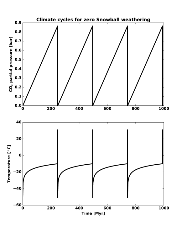
Figure 5: Timeseries of CO₂ partial pressure and temperature for the limit cycle depicted in phase space in Figure 4. Most of the limit cycle is spent in the Snowball state, during which the CO₂ increases linearly in the atmosphere. I have made this plot based on the analytical expressions in section 4: exploiting the constant CO₂ accumulation in the Snowball state, a warm state CO₂ given by Equation (18), temperature jumps at constant CO₂ for the transitions between states, and using Equations (13) and (14) to find the temperatures from the CO₂ values.

It is more difficult to calculate the time spent in the warm climate state if we let $\frac{dP}{dt}$ vary. Substituting into Equation (3) we find the following differential equation for the CO₂ partial pressure in the warm state ($\tilde{P_{w}}$)

$$\frac{d\tilde{P_{w}}}{dt}=V-W_{0}e^{k(\tilde{T_{w}}-T_{0})}\left(\frac{\tilde{P_{w}}}{P_{0}}\right)^{\beta}=V-W_{0}e^{\frac{k}{4a}(S-S_{0})(1-\alpha_{w})}\left(\frac{\tilde{P_{w}}}{P_{0}}\right)^{\beta+\frac{kb}{a}}.$$ (17)

Equation (17) has a simple analytical solution for $\beta+\frac{kb}{a}$=1, which happens to be the case for our default parameters (Table 1). I will use this limit to illustrate the behavior of the warm state CO₂ drawdown. The initial condition is $\tilde{P_{w}}(t=0)=\tilde{P_{c}}(T_{i})$, so that Equation (17) is solved by

$$\tilde{P_{w}}(t)=(\tilde{P_{c}}(T_{i})-\frac{V}{W_{0}}P_{0}e^{\frac{k}{4a}(S_{0}-S)(1-\alpha_{w})})e^{-\frac{W_{0}}{P_{0}}e^{\frac{k}{4a}(S-S_{0})(1-\alpha_{w})}t}+\frac{V}{W_{0}}P_{0}e^{\frac{k}{4a}(S_{0}-S)(1-\alpha_{w})}.$$ (18)

We are seeking the time, $\tau_{w}$, such that $\tilde{P_{w}}(t=\tau_{w})=\tilde{P_{w}}(T_{i})$, so plugging into Equation (18) we find

$$\tau_{w2}=\frac{P_{0}}{W_{0}}e^{\frac{k}{4a}(S_{0}-S)(1-\alpha_{w})}\log\left(\frac{\tilde{P_{c}}(T_{i})-\frac{V}{W_{0}}P_{0}e^{\frac{k}{4a}(S_{0}-S)(1-\alpha_{w})}}{\tilde{P_{w}}(T_{i})-\frac{V}{W_{0}}P_{0}e^{\frac{k}{4a}(S_{0}-S)(1-\alpha_{w})}}\right).$$ (19)

In general $\tau_{c}\gg\tau_{w1}>\tau_{w2}$, as we would expect because the temperatures are high and the weathering is fast in the warm state (leading to a low $\tau_{w2}$) and we limit the weathering rate in our other warm state timescale estimate ($\tau_{w1}$). For example, for the parameters used in Figure (4), $\tau_{c}$=250 Myr (slow), the two estimates for the time spent in the warm state are $\tau_{w1}$=5 Myr and $\tau_{w2}$=0.5 Myr (fast), and the time to transition between the warm and Snowball states ($\frac{C}{a}$) is about 3 years (very fast).

Since the other components of the cycle take are short, $\tau_{c}$ (Equation (15)) yields a good approximation of the period of the total cycle, which we will call $\tau$. We can drop the constants associated with the reference state in Equation (15) as follows to think about the variable dependencies of $\tau$

$$\tau\propto\frac{1}{V}e^{\frac{a}{b}T_{i}-\frac{S}{4b}(1-\alpha_{c})}.$$ (20)

As one might expect, the period of the cycles is inversely proportional to the CO₂ outgassing rate. The more interesting aspect of Equation (20) is that it gives us a functional form for the dependence of the period of the cycle on the stellar flux and albedo of the cold state. If we start in the warm state and decrease the stellar flux (say by moving the planet away from the star), a limit cycle will suddenly appear when the threshold for existence of the warm state is crossed (Equation (6)). If we continue to decrease the stellar flux, the period of this cycle will grow exponentially as the stellar flux is decreased. The exponential functional dependence ultimately derives from the logarithmic effect of CO₂ on infrared emission to space (Equation (1)). This means that the period of the cycle for planets near the outer edge of the habitable zone will be very long, so the difference between having a permanent Snowball state as in section 3 and having very slow cycles through the Snowball and warm states as described in this section will be marginal. Similarly, the timescales will be exponentially shorter as we decrease the Snowball albedo. Since ice and snow have a much lower albedo for an M-star spectrum (Joshi & Haberle, 2012; Shields et al., 2013), this implies that the climate cycles for planets in M-star systems would have much shorter periods. Finally, increasing $b$ decreases the effect of changing the stellar flux and Snowball albedo. It is important to note that since we have set the weathering rate to zero in the Snowball, which is the part of the cycle that determines its period, none of the uncertain weathering parameters affect the period of the cycle.

The dependence of $\tau$ on $T_{i}$ (Equation (20) can significantly affect the comparison of different models. For example, I implemented a smoothed version of the albedo transition (Equation (2)) and integrated the system numerically. I found that the period of the cycle was strongly dependent on the temperature smoothing of the albedo parameterization because this affected the effective temperature at which the transition from the Snowball to the warm climate occurred. Using $\frac{a}{b}=0.2$, a decrease in $T_{i}$ by about 10 K leads to a decrease in $\tau$ by about an order of magnitude. This sensitivity will affect the comparison of cycle periods between models, however, the dependencies shown in Equation (20) should hold within a given model.

We can use Equation (20) to understand simulations in more complex models. For example, Menou (2015) performed six different simulations of climate cycles for planets at different orbital distances (corresponding to different stellar fluxes), CO₂ outgassing rates, and values of $\beta$. Two of these simulations have a CO₂ outgassing rate three times higher than the others, and, according to Equation (20), I have adjusted their period by multiplying it by three. I have plotted the logarithm of the adjusted period as a function of stellar flux in Figure 6. I have also plotted the time spent in the Snowball state for each simulation, which we can calculate because Menou (2015) gives the percentage of the cycle spent in the warm state. The first thing to note is that the logarithm of the period is fairly linear in stellar flux, consistent with Equation (20). If we assume that the Snowball albedo is 0.7, the slope of the line corresponds to a value of $b$ of about 27 W m^-2, which is the right order of magnitude. Two of the simulations have periods 10–20% longer than expected. These simulations have a lower value of $\beta$, and therefore spend a higher fraction of their cycle in the warm state (Menou, 2015). We should also note that even the time spent in the Snowball state does not fall exactly on a straight line, and it is not a single-valued function of stellar flux. The reasons for this are: (1) Menou (2015) uses a much more complex radiation model in which infrared emission to space is not simply a linear function of the logarithm of CO₂, (2) Menou (2015) calculates the Snowball albedo including the effect of the amount of CO₂, so it is not a constant, and (3) the weathering parameterization that Menou (2015) uses allows some weathering for temperatures slightly below the Snowball deglaciation temperature threshold, which can delay the deglaciation and causes different results for different values of $\beta$. Despite these differences, Equation (20) does an excellent job of describing the qualitative behavior of period of the cycles from the simulations of Menou (2015).

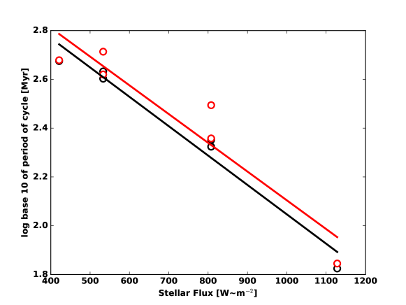
Figure 6: Logarithm of the period of the climate cycles from Menou (2015) (red circles) and time in the Snowball state (black circles) as a function of stellar flux. Lines of best fit, with corresponding colors, are also shown. Two of the simulations from Menou (2015) have a CO₂ outgassing rate three times higher than the other simulations, and I adjusted the period of these simulations by multiplying it by three.

5 Discussion

A major advance of this paper is to derive an explicit formula for the effective outer edge of the habitable zone (Equation 6). Although the weathering parameters in this formula are uncertain, it could be incorporated into future probabilistic estimates of habitability of discovered exoplanets, with appropriate prior distributions placed on weathering parameters. Once a planet is beyond this limit, I have found that it will either experience a permanent Snowball state or long cycles between a Snowball and warm climate, depending on whether weathering goes completely to zero during the Snowball or note. Either way the habitability of the planet would be greatly reduced. Also, the fact that the Snowball episodes Earth has experienced did end does not imply that the weathering was zero during them (Le Hir et al., 2008), since the stellar flux was relatively high during these episodes.

Kopparapu et al. (2014) found that the outer edge of the traditional habitable zone has only a small dependence on planet size, but the effective outer edge of the habitable zone could strongly depend on planet size. A larger planet will tend to have a higher rate of volcanism, and presumably CO₂ outgassing, yet it will also have a larger overburden pressure for a given volatile inventory (Kite et al., 2009). These competing effects will determine how planetary size affects CO₂ outgassing rate, and consequently susceptibility to loss of the warm climate state inside the traditional habitable zone. Moreover, the CO₂ outgassing rate should decrease strongly with time (Kite et al., 2009), which indicates that planets near the outer edge of the traditional habitable zone are more likely to actually be habitable in younger systems.

The albedo and thermal phase curve of an Earth-like planet could be interrogated to determine whether it was in a Snowball or warm climate state (Cowan et al., 2012). This might be possible for a planet near the outer edge of the habitable zone with the James Webb Space Telescope (Yang et al., 2013; Koll & Abbot, 2015), and would certainly be possible with a future mission such as the High Definition Space Telescope (Dalcanton et al., 2015). New geochronological data (Condon et al., 2016) suggest that the Sturtian and Marinoan Snowball Earth episodes had a combined duration of about 80 Myr, which is about 10% of the time since they occurred, implying that a roughly 10% Snowball duty cycle could be realistic for an Earth-like planet. Planets near the outer edge of the traditional habitable zone that have a stable warm state but are perturbed away from it and into a Snowball could take longer to warm up via CO₂ outgassing and will therefore spend a somewhat higher percentage of their time as a Snowball. If these planets are anything like Earth, however, they should still spend the vast majority of their time in the warm climate state. Planets outside the effective outer edge of the habitable zone, on the other hand, should spend most of their time as a Snowball. Therefore a measurement of the fraction of Earth-like planets in a warm state as a function of position in the habitable zone would tell us whether CO₂-outgassing limitations on the habitable zone are important. A large increase in the average number of Earth-like planets in a Snowball state near the outer edge of the habitable zone would indicate that CO₂-outgassing limitations are important on average. In this way astronomical measurements could increase our understanding of weathering. Similarly, continued study of river catchments, paleoclimate, and laboratory weathering analogs should help improve our understanding of weathering, and therefore the effective outer edge of the habitable zone, which will inform the astronomical search for habitable exoplanets.

In this paper I have not included the effect of CO₂ on planetary albedo. This means that if the weathering is set to zero in a Snowball state, then the CO₂ can always build up to high enough values to cause deglaciation and lead to climate cycles if the warm state does not exist (section 4). For Snowball states that require tens of bars of CO₂ to deglaciate, increased shortwave scattering by CO₂ could prevent deglaciation from ever occurring. If this were the case, the Snowball state could be stable even if the CO₂ cycle is not balanced. If deglaciaton does occur at a very high CO₂ level, then the atmospheric albedo might be so high that the change in surface albedo has a minimal effect on the planetary albedo (Wordsworth et al., 2011), so the warming associated with deglaciation is minimal. In this case CO₂ could still be drawn down due to high CO₂ concentrations (Equation (3)), leading to a climate cycle, but the planet would likely spend more time in the warm state.

Finally, we should note that even if the effective outer edge of the habitable zone occurs at a significantly higher stellar flux than the traditional outer edge, there should still be plenty of habitats for life in the universe. If the habitable zone were cut in half, the proportion of Sun-like stars hosting Earth-like potentially habitable planets would go from $\sim$5% to $\sim$2.5% (Petigura et al., 2013), which might have been considered an optimistic estimate before the Kepler mission. Moreover, recent work on H₂-greenhouse planets suggests that habitable planets can exist even outside of the traditional habitable zone (Stevenson, 1999; Pierrehumbert & Gaidos, 2011; Wordsworth, 2012; Abbot, 2015). Additionally, life, and maybe even animal life, seems to have survived the Snowball Earth episodes, and could potentially survive permanent or cyclical Snowball climates near the outer edge of the habitable zone, although such conditions would certainly be less favorable to complex life than modern Earth. Finally, if simple life can exist in subglacial oceans on distant or unbound Earth-like planets (Laughlin & Adams, 2000; Abbot & Switzer, 2011), then the Snowball planets beyond the effective habitable zone would still be viable hosts for some sort of life.

6 Conclusions

The main conclusions of this paper are:

1. The stellar flux at the effective outer edge of the habitable zone can be approximated by the following formula:

   $$S^{\ast}=S_{0}-\left(\frac{4}{1-\alpha_{w}}\right)\left(\frac{b}{\beta}\log\left(\frac{V}{W_{0}}\right)+k(T_{0}-T_{i})(\frac{b}{\beta}+\frac{a}{k})\right).$$

   Larger values of $k$, the weathering-temperature rate constant, linearly decrease the stellar flux of the effective outer edge of the habitable zone, moving it farther from the star and providing more habitable space in the system. Smaller values of $\beta$, the weathering-CO₂ power law exponent, directly decrease the stellar flux of the effective outer edge of the habitable zone and also leverage the effect of increases in the CO₂ outgassing rate. If $k$ is increased by about a factor of two or $\beta$ is decreased by a factor of two, or some smaller combination of the two, then the effective outer edge of the habitable zone equals the traditional outer edge of the habitable zone even for modern Earth’s CO₂ outgassing rate, and none of the habitable zone would be lost. These changes are within the uncertainty in the values of $k$ and $\beta$. This equation also tells us that M-star planets should tend to have less of a reduction in their habitable zone due to limited CO₂ outgassing, since $\alpha_{w}$, the warm state albedo, will tend to be smaller for M-star planets (making $S^{\ast}$ smaller).

   The formula for $S^{\ast}$ could be incorporated into probabilistic estimates of whether a discovered exoplanet is habitable, using appropriate priors on $k$ and $\beta$. It could similarly be used to estimate the fraction of stars that host an Earth-like planet given statistics of exoplanet occurrences. Both of these uses would aid in the planning of telescopes that would observe Earth-like planets and search for biosignatures.

2. Beyond the effective outer edge of the habitable zone (but inside the traditional outer edge) cycles between a Snowball and warm climate are possible if weathering is weak enough that the CO₂ needed to deglaciate a Snowball is reached before weathering can balance CO₂ outgassing (for example if the weathering rate is simply set to zero in a Snowball climate). If weathering occurs either subglacially or at the seafloor, it is possible to have a stable, attracting Snowball climate state.

3. If climate cycles between a Snowball and warm state occur, then the period of these cycles scales as

   $$\tau\propto\frac{1}{V}e^{\frac{a}{b}T_{i}-\frac{S}{4b}(1-\alpha_{c}))}.$$

   This formula comes from the time spent in the Snowball state, which dominates the total period and can be calculated by dividing the CO₂ needed to deglaciate the Snowabll by the CO₂ outgassing rate (which explains why the period of the cycles is inversely proportional to the CO₂ outgassing rate). The exponential dependence on the temperature at which the Snowball state deglaciates and the negative exponential dependence on the stellar flux ultimately derive from the fact that CO₂ has a logarithmic effect on infrared emission to space and the greenhouse warming of a planet. The negative exponential dependence on stellar flux indicates that cycles near the outer edge of the habitable zone will have very long periods, and may be hard to distinguish from permanent Snowball states. The exponential dependence on the planetary albedo of the cold state indicates that climate cycles will have a shorter period for planets orbiting M-stars because the albedo of ice and snow is lower for an M-star spectrum. Finally, it is important to note that none of the uncertain weathering parameters appear in this scaling.

7 Acknowledgements

I acknowledge support from the NASA Astrobiology Institute’s Virtual Planetary Laboratory, which is supported by NASA under cooperative agreement NNH05ZDA001C. I thank Navah Farahat for helping me learn python plotting routines. I thank Cael Berry, Edwin Kite, Daniel Koll, Mary Silber, and Robin Wordsworth for reading an early draft of this paper and providing detailed and insightful suggestions.

References

- Abbot (2015) Abbot, D. S. 2015, Astrophysical Journal Letters, 815, L3
- Abbot et al. (2012) Abbot, D. S., Cowan, N. B., & Ciesla, F. J. 2012, Astrophysical Journal, 756, 178, doi:10.1088/0004-637X/756/2/178
- Abbot & Switzer (2011) Abbot, D. S., & Switzer, E. R. 2011, Astrophysical Journal, 735, L27, doi:10.1088/2041-8205/735/2/L27
- Abbot et al. (2011) Abbot, D. S., Voigt, A., & Koll, D. 2011, Journal of Geophysical Research, 116, D18103, doi:10.1029/2011JD015927
- Berner (1994) Berner, R. 1994, Am J Sci, 294, 56
- Berner (2004) Berner, R. A. 2004, The Phranerozoic Carbon Cycle (Oxford University Press, New York, N.Y.)
- Condon et al. (2016) Condon, D., Macdonald, F. A., Rooney, A. D., Zhu, M., Schmitz, M. D., & Bowring, S. A. 2016, Sci. Adv., submitted
- Cowan et al. (2012) Cowan, N. B., Abbot, D. S., & Voigt, A. 2012, Astrophysical Journal, 757, 80, doi:10.1088/0004-637X/757/1/80
- Dalcanton et al. (2015) Dalcanton, J., et al. 2015, arXiv preprint arXiv:1507.04779
- Dasgupta (2013) Dasgupta, R. 2013, Rev Mineral Geochem, 75, 183
- Foley (2015) Foley, B. J. 2015, The Astrophysical Journal, 812, 36
- Goldblatt et al. (2013) Goldblatt, C., Robinson, T. D., Zahnle, K. J., & Crisp, D. 2013, Nature Geoscience, 6, 661
- Goldblatt & Watson (2012) Goldblatt, C., & Watson, A. J. 2012, Philosophical Transactions Of The Royal Society A-Mathematical Physical And Engineering Sciences, 370, 4197
- Gough (1981) Gough, D. O. 1981, Sol Phys, 74, 21
- Grott et al. (2011) Grott, M., Morschhauser, A., Breuer, D., & Hauber, E. 2011, Earth and Planetary Science Letters, 308, 391
- Halevy & Head III (2014) Halevy, I., & Head III, J. W. 2014, Nature Geoscience, 7, 865
- Haqq-Misra et al. (2016) Haqq-Misra, J., Kopparapu, R. K., Batalha, N. E., Harman, C. E., & Kasting, J. F. 2016, arXiv preprint arXiv:1605.07130
- Hoffman et al. (1998) Hoffman, P. F., Kaufman, A. J., Halverson, G. P., & Schrag, D. P. 1998, Science, 281, 1342
- Huybers & Langmuir (2009) Huybers, P., & Langmuir, C. 2009, Earth and Planetary Science Letters, 286, 479
- Joshi & Haberle (2012) Joshi, M. M., & Haberle, R. M. 2012, Astrobiology, 12, 3
- Kadoya & Tajika (2014) Kadoya, S., & Tajika, E. 2014, The Astrophysical Journal, 790, 107
- Kasting (1988) Kasting, J. F. 1988, Icarus, 74, 472
- Kasting et al. (1993) Kasting, J. F., Whitmire, D. P., & Reynolds, R. T. 1993, Icarus, 101, 108
- Kirschvink (1992) Kirschvink, J. 1992, in The Proterozoic Biosphere: A Multidisciplinary Study, ed. J. Schopf & C. Klein (Cambridge University Press, New York), 51–52
- Kite et al. (2009) Kite, E., Manga, M., & Gaidos, E. 2009, Astrophys Journal, 700, 1732, doi:10.1088/0004-637X/700/2/1732
- Kite et al. (2015) Kite, E. S., Howard, A. D., Lucas, A. S., Armstrong, J. C., Aharonson, O., & Lamb, M. P. 2015, Icarus, 253, 223
- Koll & Abbot (2015) Koll, D. D. B., & Abbot, D. S. 2015, The Astrophysical Journal, 802, 21, doi:10.1088/0004-637X/802/1/21
- Kopparapu (2013) Kopparapu, R. K. 2013, Astrophysical Journal Letters, 767, L8
- Kopparapu et al. (2014) Kopparapu, R. K., Ramirez, R. M., SchottelKotte, J., Kasting, J. F., Domagal-Goldman, S., & Eymet, V. 2014, The Astrophysical Journal Letters, 787, L29
- Kopparapu et al. (2013) Kopparapu, R. K., et al. 2013, The Astrophysical Journal, 765, 131
- Laughlin & Adams (2000) Laughlin, G., & Adams, F. 2000, Icarus, 145, 614
- Le Hir et al. (2008) Le Hir, G., Ramstein, G., Donnadieu, Y., & Godderis, Y. 2008, Geology, 36, 47
- Leconte et al. (2013a) Leconte, J., Forget, F., Charnay, B., Wordsworth, R., & Pottier, A. 2013a, Nature, 504, 268
- Leconte et al. (2013b) Leconte, J., Forget, F., Charnay, B., Wordsworth, R., Selsis, F., Millour, E., & Spiga, A. 2013b, Astronomy And Astrophysics, 554, A69
- Menou (2015) Menou, K. 2015, Earth and Planetary Science Letters, 429, 20
- Mills et al. (2011) Mills, B., Watson, A. J., Goldblatt, C., Boyle, R., & Lenton, T. M. 2011, Nature Geosciences, 4, 861, DOI: 10.1038/NGEO1305
- Nakajima et al. (1992) Nakajima, S., Hayashi, Y. Y., & Abe, Y. 1992, Journal of the Atmospheric Sciences, 49, 2256
- Petigura et al. (2013) Petigura, E. A., Howard, A. W., & Marcy, G. W. 2013, Proceedings of the National Academy of Sciences, 110, 19273
- Pierrehumbert & Gaidos (2011) Pierrehumbert, R., & Gaidos, E. 2011, Astrophys J Lett, 734, L13, doi:10.1088/2041-8205/734/1/L13
- Pierrehumbert (2010) Pierrehumbert, R. T. 2010, Principles of Planetary Climate (Cambridge University Press)
- Rose (2015) Rose, B. E. 2015, Journal of Geophysical Research: Atmospheres, 120, 1404
- Shields et al. (2013) Shields, A. L., Meadows, V. S., Bitz, C. M., Pierrehumbert, R. T., Joshi, M. M., & Robinson, T. D. 2013, Astrobiology, 13, 715
- Stevenson (1999) Stevenson, D. J. 1999, Nature, 400, 32, doi:10.1038/21811
- Strogatz (1994) Strogatz, S. 1994, Nonlinear dynamics and chaos (Westview Press)
- Tajika (2007) Tajika, E. 2007, Earth, 59, 293
- Voigt & Abbot (2012) Voigt, A., & Abbot, D. S. 2012, Climate of the Past, 8, 2079, doi:10.5194/cp-8-2079-2012
- Voigt et al. (2011) Voigt, A., Abbot, D. S., Pierrehumbert, R. T., & Marotzke, J. 2011, Clim. Past, 7, 249, doi:10.5194/cp-7-249-2011
- Walker et al. (1981) Walker, J. C. G., Hays, P. B., & Kasting, J. F. 1981, Journal of Geophysical Research, 86, 9776
- West et al. (2005) West, A. J., Galy, A., & Bickle, M. 2005, Earth and Planetary Science Letters, 235, 211
- Wolf & Toon (2014) Wolf, E., & Toon, O. 2014, Geophysical Research Letters, 41, 167–172, dOI: 10.1002/2013GL058376
- Wolf & Toon (2015) —. 2015, Journal of Geophysical Research, 120, 5775
- Wordsworth (2012) Wordsworth, R. 2012, Icarus, 219, 267, doi:10.1016/j.icarus.2012.02.035
- Wordsworth et al. (2013) Wordsworth, R., Forget, F., Millour, E., Head, J. W., Madeleine, J. B., & Charnay, B. 2013, Icarus, 222, 1
- Wordsworth et al. (2011) Wordsworth, R. D., Forget, F., Selsis, F., Millour, E., Charnay, B., & Madeleine, J.-B. 2011, Astrophys J Lett, 733, L48, doi:10.1088/2041-8205/733/2/L48
- Yang et al. (2014) Yang, J., Boué, G., Fabrycky, D. C., & Abbot, D. S. 2014, Astrophysical Journal Letters, 787, L2, doi:10.1088/2041-8205/787/1/L2
- Yang et al. (2013) Yang, J., Cowan, N. B., & Abbot, D. S. 2013, Astrophysical Journal Letters, 771, L45, DOI:10.1088/2041-8205/771/2/L45
- Yang et al. (2012a) Yang, J., Peltier, W., & Hu, Y. 2012a, Journal of Climate, 25, 2711, doi: 10.1175/JCLI-D-11-00189.1
- Yang et al. (2012b) —. 2012b, Journal of Climate, 25, 2737, doi: 10.1175/JCLI-D-11-00190.1
- Yang et al. (2012c) Yang, J., Peltier, W. R., & Hu, Y. 2012c, Climate of the Past, 8, 907, doi:10.5194/cp-8-907-2012