Stabilization of Second Order Nonlinear Equations with Variable Delay

Abstract

For a wide class of second order nonlinear non-autonomous models, we illustrate that combining proportional state control with the feedback that is proportional to the derivative of the chaotic signal, allows to stabilize unstable motions of the system. The delays are variable, which leads to more flexible controls permitting delay perturbations; only delay bounds are significant for stabilization by a delayed control. The results are applied to the sunflower equation which has an infinite number of equilibrium points.

1 Introduction

It is well known that control of dynamical systems is a classical subject in engineering sciences. Time delayed feedback control is an efficient method for stabilizing unstable periodic orbits of chaotic systems which are described by second order delay differential equations, see Botmart (2012); Dombovari (2011); French (2009); Freitas (2000); Kim (2013); Liu (2010); Reithmeier (2003); Stepan (2009); Szalai (2010); Wan (2010). When introducing a control, we assume that the chosen equilibrium of an equation is unstable, and the controller will transform the unstable equation into an asymptotically or exponentially stable equation. Instability tests for some autonomous delay models of the second order could be found, for example, in Cahlon (2004). Two basic proportional (adaptive) control models are widely used: standard feedback controllers $u(t)=K[x(t)-x^{\ast}]$ with the controlling force proportional to the deviation of the system from the attractor, where $x^{\ast}$ is an equilibrium of the equation, and the delayed feedback control $u(t)=K[x(t-\tau(t))-x(t)]$, see Boccaletti (2000); Johnston (1993); Konishi (2011).

Proportional control fails if there exist rapid changes to the system that come from an external source, and to keep the system steady under an abrupt change, a derivative control was used in Bielawski (1994); Reithmeier (2003); Vyhlial (2009), i.e. $u(t)=\beta\frac{d}{dt}e(t)$, where, for example, $e(t)=x(t-\tau)-x(t)$ or $e(t)=x(t)-x^{\ast}$. In electronics, a simple operational amplifier differentiator circuit will generate the continuous feedback signal which is proportional to the time derivative of the voltage across the negative resistance, see Johnston (1993). A classical proportional control does not stabilize even linear ordinary differential equations; e.g. the equation $\ddot{x}=u(t)$ with the control $u(t)=K[x(t-\tau(t))-x(t)]$ is not asymptotically stable for any $K$, since any constant is a solution of this equation. The pure derivative control $u(t)=-\lambda\dot{x}(t)$ also does not stabilize all second order differential equations. For example, the equation $\ddot{x}+ax(t)-ax(t-\tau)=u(t)$ with the control $u(t)=-\lambda\dot{x}(t)$ is not asymptotically stable for any control since any constant is a solution of this equation. Some interesting and novel results could be found in Ren (2009); Rusinek (2014); Sipahi (2011); Wang (2013); Yan (2011). For a linear non-autonomous model $\dot{x}=A(t)x(t)+B(t)u(t)$ the effective multiple-derivative feedback controller $\displaystyle u(t)=\sum_{i=0}^{M-1}K_{i}x^{(i)}(t-h)$ was introduced in Stoorvogel (2010), and a special transformation was used to transform neutral-type DDE into a retarded DDE. However, most of second order applied models are nonlinear, even the original pendulum equation. The main focus of the paper is the control of nonlinear delay equations, some real world models are considered in Examples 2.9,3.2,3.3.

In the present paper we study a nonlinear second order delay differential equation

$$\ddot{x}(t)+\sum_{k=1}^{l}f_{k}(t,\dot{x}(g_{k}(t)))+\sum_{k=1}^{m}s_{k}(t,x(h_{k}(t)))=u(t),~{}~{}t\geq t_{0},$$ (1.1)

with the input or the controller $u(t)$, along with its linear version

$$\ddot{x}(t)+\sum_{k=1}^{l}a_{k}(t)\dot{x}(g_{k}(t))+\sum_{k=1}^{m}b_{k}(t)x(h_{k}(t))=u(t),~{}~{}t\geq t_{0}.$$ (1.2)

Both equations (1.2) and (1.1) satisfy for any $t_{0}\geq 0$ the initial condition

$$x(t)=\varphi(t),~{}\dot{x}(t)=\psi(t),~{}t\leq t_{0}.$$ (1.3)

We will assume that the initial value problem has a unique global solution on $[t_{0},\infty)$ for all nonlinear equations considered in this paper, and the following conditions are satisfied:
(a1) $a_{i},b_{j}$ are Lebesgue measurable and essentially bounded on $[0,\infty)$ functions, $i=1,\dots,l$, $j=1,\dots,m$, which allows to define essential eventual limits

$$\alpha=\limsup_{t\rightarrow\infty}\sum_{k=1}^{l}|a_{k}(t)|,~{}\beta=\limsup_{t\rightarrow\infty}\sum_{k=1}^{m}|b_{k}(t)|;$$ (1.4)

(a2) $h_{j},g_{i}$ are Lebesgue measurable functions, $h_{i}(t)\leq t,g_{i}(t)\leq t,$ $\lim\limits_{t\to\infty}h_{i}(t)=\infty$, $\lim\limits_{t\to\infty}g_{i}(t)=\infty$, $i=1,\dots,l$, $j=1,\dots,m$.

The paper is organized as follows. In Section 2 we design a stabilizing damping control $u(t)=\lambda_{1}\dot{x}(t)+\lambda_{2}(x(t)-x^{*})$ for any linear non-autonomous equation (1.2). Under some additional condition on the functions $f_{k}$ and $s_{k}$, such control also stabilizes equations of type (1.1). The results are based on stability tests recently obtained in Berezansky (2008, arXiv,2014) for second order non-autonomous differential equations. We also prove in Section 2 that a strong enough controlling force, depending on the derivative and the present (and past) positions, can globally stabilize an equilibrium of the controlled equation. In Section 3 classical proportional delayed feedback controller $u(t)=K[x(t-\tau(t))-x(t)]$ is applied to stabilize a certain class of second order delay equations with a single delay involved in the state term only. We develop tailored feedback controllers and justify their application both analytically and numerically.

2 Damping Control

We will use auxiliary results recently obtained in Berezansky (2008, arXiv,2014).

Lemma 2.1.

(Berezansky, 2008, Corollary 3.2) If $a>0,b>0,$

$$4b>a^{2},~{}~{}\frac{2(a+\sqrt{4b-a^{2}})}{a\sqrt{4b-a^{2}}}\alpha+\frac{4}{a\sqrt{4b-a^{2}}}\beta<1,$$ (2.1)

where $\alpha$ and $\beta$ are defined in (a1) by (1.4), then the zero solution of the equation

$$\ddot{x}(t)+a\dot{x}(t)+bx(t)+\sum_{k=1}^{l}a_{k}(t)\dot{x}(g_{k}(t))+\sum_{k=1}^{m}b_{k}(t)x(h_{k}(t))=0$$ (2.2)

is globally exponentially stable.

Lemma 2.2.

Berezansky (arXiv,2014) Assume that the equation

$$\ddot{x}(t)+f(t,x(t),\dot{x}(t))+s(t,x(t))+\sum_{k=1}^{m}s_{k}(t,x(t),x(h_{k}(t)))=0$$ (2.3)

possesses a unique trivial equilibrium, where $f(t,v,0)=0$, $s(t,0)=0$, $s_{k}(t,v,0)=0$,
$0<a_{0}\leq\frac{f(t,v,u)}{u}\leq A$, $\displaystyle 0<b_{0}\leq\frac{s(t,u)}{u}\leq B$, $\displaystyle\left|\frac{s_{k}(t,v,u)}{u}\right|\leq C_{k},u\neq 0,~{}t-h_{k}(t)\leq\tau$.

If at least one of the conditions
1) $\displaystyle B\leq\frac{a_{0}^{2}}{4},~{}\sum_{k=1}^{m}C_{k}<b_{0}-\frac{a_{0}}{2}(A-a_{0})$,        2) $\displaystyle b_{0}\geq\frac{a_{0}}{2}\left(A-\frac{a_{0}}{2}\right),~{}\sum_{k=1}^{m}C_{k}<\frac{a_{0}^{2}}{2}-B$
holds, then zero is a global attractor for all solutions of equation (2.3).

We start with linear equations. Stabilization results for linear systems were recently obtained in Stoorvogel (2010); Wang (2013). Unlike Stoorvogel (2010); Wang (2013), the following theorem considers models with variable delays, however, the control is not delayed.

Theorem 2.3.

For any $\delta\in(0,2)$, $\alpha$ and $\beta$ defined by (1.4) and

$$\lambda>\mu(\lambda):=\frac{(\delta+\sqrt{4-\delta^{2}})\alpha+\sqrt{(\delta+\sqrt{4-\delta^{2}})^{2}\alpha^{2}+4\sqrt{4-\delta^{2}}\beta\delta}}{\delta\sqrt{4-\delta^{2}}}\,,$$ (2.4)

equation (1.2) with the control $u(t)=-\delta\lambda\dot{x}(t)-\lambda^{2}x(t)$ is exponentially stable.

Proof.

Equation (1.2) with the control

$$\ddot{x}(t)+\sum_{k=1}^{l}a_{k}(t)\dot{x}(g_{k}(t))+\sum_{k=1}^{m}b_{k}(t)x(h_{k}(t))=-\delta\lambda\dot{x}(t)-\lambda^{2}x(t)$$ (2.5)

has the form of (2.2) with $a=\delta\lambda$ and $b=\lambda^{2}$. Then the inequalities in (2.1) have the form

$$4\lambda^{2}>\delta^{2}\lambda^{2}\mbox{~{}~{}and~{}~{}}\frac{2(\delta+\sqrt{4-\delta^{2}})}{\delta\lambda\sqrt{4-\delta^{2}}}\alpha+\frac{4}{\delta\lambda^{2}\sqrt{4-\delta^{2}}}\beta<1.$$ (2.6)

The first inequality in (2.6) holds as $\delta\in(0,2)$, and the second one is equivalent to

$$\delta\lambda^{2}\sqrt{4-\delta^{2}}-2\left(\delta+\sqrt{4-\delta^{2}}\right)\alpha\lambda-4\beta>0.$$ (2.7)

Condition (2.4) implies (2.7), which completes the proof. ∎

Corollary 2.4.

Let $\displaystyle\mu(\delta_{0})=\min_{\delta\in[\varepsilon,2-\varepsilon]}\mu(\delta)$ for some $\varepsilon>0$, where $\mu(\delta)$ is defined in (2.4). Then for $\lambda>\mu(\delta_{0})$ equation (1.2) with the control $u(t)=-\delta_{0}\lambda\dot{x}(t)-\lambda^{2}x(t)$ is exponentially stable.

For $\delta=\sqrt{2}$ Theorem 2.3 yields the following result.

Corollary 2.5.

Eq. (1.2) with the control $u(t)=-\sqrt{2}\lambda\dot{x}(t)-\lambda^{2}x(t)$ is exponentially stable if

$$\lambda>\sqrt{2}(\alpha+\sqrt{\alpha^{2}+\beta}).$$ (2.8)

Remark 2.6.

For any equation (1.2) there exists $\lambda>0$ such that condition (2.8) holds. Hence the stabilizing damping control exists for any equation of form (1.2).

Example 2.7.

For the equation

$$\ddot{x}(t)+(\sin t)\dot{x}(g(t))+(\cos t)x(h(t))=0,~{}~{}h(t)\leq t,~{}g(t)\leq t,$$ (2.9)

the upper bounds defined in (1.4) are $\alpha=\beta=1$. Hence, as long as $\lambda>2+\sqrt{2}$ in Corollary 2.5, equation (2.9) with the control $u(t)=-\sqrt{2}\lambda\dot{x}(t)-\lambda^{2}x(t)$ is exponentially stable.

Let us proceed to nonlinear equation (1.1); its stabilization is the main object of the present paper. For simplicity we consider here nonlinear equations with the zero equilibrium, since the change of the variable $z=x-x^{\ast}$ transforms an equation with the equilibrium $x^{*}$ into an equation in $z$ with the zero equilibrium.

Theorem 2.8.

Suppose $f_{k}(t,0)=s_{k}(t,0)=0$,

$$\left|\frac{f_{k}(t,u)}{u}\right|\leq a_{k}(t),~{}\left|\frac{s_{k}(t,u)}{u}\right|\leq b_{k}(t),u\neq 0.$$ (2.10)

Then for any $\delta\in(0,2)$, the zero equilibrium of (1.1) with the control $u(t)=-\delta\lambda\dot{x}(t)-\lambda^{2}x(t)$

$$\ddot{x}(t)+\sum_{k=1}^{l}f_{k}(t,\dot{x}(g_{k}(t)))+\sum_{k=1}^{m}s_{k}(t,x(h_{k}(t)))=-\delta\lambda\dot{x}(t)-\lambda^{2}x(t)$$ (2.11)

is globally asymptotically stable, provided (2.4) holds with $\alpha$ and $\beta$ defined in (1.4).

Proof.

Suppose $x$ is a fixed solution of equation  (2.11). Equation (2.11) can be rewritten as

$$\ddot{x}(t)+\sum_{k=1}^{l}a_{k}(t)\dot{x}(g_{k}(t))+\sum_{k=1}^{m}b_{k}(t)x(h_{k}(t))=-\delta\lambda\dot{x}(t)-\lambda^{2}x(t),$$

where $\displaystyle a_{k}(t)=\left\{\begin{array}[]{cc}\frac{f_{k}(t,\dot{x}(t))}{\dot{x}(t)},&\dot{x}(t)\neq 0,\\ 0,&\dot{x}(t)=0,\end{array}\right.~{}~{}b_{k}(t)=\left\{\begin{array}[]{cc}\frac{s_{k}(t,x(t))}{x(t)},&x(t)\neq 0,\\ 0,&x(t)=0.\end{array}\right.$    Hence the function $x$ is a solution of the linear equation

$$\ddot{y}(t)+\sum_{k=1}^{l}a_{k}(t)\dot{y}(g_{k}(t))+\sum_{k=1}^{m}b_{k}(t)y(h_{k}(t))=-\delta\lambda\dot{y}(t)-\lambda^{2}y(t),$$ (2.12)

which is exponentially stable by Theorem 2.3. Thus $\lim\limits_{t\rightarrow\infty}y(t)=0$ for any solution $y$ of equation (2.12), and since $x$ is a solution of (2.12), $\lim\limits_{t\rightarrow\infty}x(t)=0.$ ∎

In particular, for $\delta=\sqrt{2}$ condition (2.4) transforms into (2.8).

Example 2.9.

Consider the equation

$$\ddot{x}(t)+a(t)\dot{x}(g(t))+b(t)\sin(x(h(t)))=0,~{}~{}h(t)\leq t,~{}g(t)\leq t,$$ (2.13)

with $|a(t)|\leq\alpha,|b(t)|\leq\beta$. Equation (2.13) generalizes the sunflower equation introduced by Israelson and Johnson in Israelson (1967) as a model for the geotropic circumnutations of Helianthus annuus; later it was studied in Casal (1982); Lizana (1999); Somolinos (1978).

We have $\displaystyle\left|\frac{\sin u}{u}\right|\leq 1,~{}u\neq 0$; hence if condition (2.8) holds for $\alpha=\limsup\limits_{t\rightarrow\infty}|a(t)|$ and $\beta=\limsup\limits_{t\rightarrow\infty}|b(t)|$, then the zero equilibrium of equation (2.13) with the control $u(t)=-\sqrt{2}\lambda\dot{x}(t)-\lambda^{2}x(t)$ in the right-hand side is globally exponentially stable. Equation (2.13) has an infinite number of equilibrium points $x^{\ast}=\pi k$, $k=0,1,\dots$. To stabilize a fixed equilibrium $x^{\ast}=\pi k$ we apply the controller $u(t)=-\sqrt{2}\lambda\dot{x}(t)-\lambda^{2}(x(t)-x^{\ast})$.

For example, consider the sunflower equation

$$\ddot{x}(t)+\dot{x}(t)+2\sin(x(t-\pi))=0$$

with various initial conditions $x(0)=6,3,0.1$, where $x(t)$ is constant for $t\leq 0$, $x^{\prime}(0)=1$ which has chaotic solutions (see Fig. 1, left). Application of the controller $u(t)=-\lambda\delta\dot{x}(t)-\lambda^{2}[x(t)-\pi]$, where $\delta=\sqrt{2}$ and $\lambda>\sqrt{2}+\sqrt{6}$, for example, $\lambda=4$, stabilizes the otherwise unstable equilibrium $x^{\ast}=\pi$, as illustrated in Fig. 1, right.

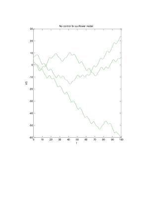
Figure 1: Stabilization of the equilibrium of the sunflower equation $\ddot{x}(t)+\dot{x}+2\sin(x(t-\pi))=0$ with various initial conditions. The left graph illustrates unstable (chaotic) solutions while in the right graph, corresponding to the sunflower model with the control $u(t)=-\lambda\delta\dot{x}(t)-\lambda^{2}[x(t)-\pi]$, all three solutions of the controlled equation converge to the equilibrium $\pi$.

3 Classical proportional control

In this section we investigate stabilization with the standard proportional delayed control.

Consider the equation

$$\ddot{x}(t)+a\dot{x}(t)+bx(h(t))=f(t,x(g(t)))$$ (3.1)

which has an equilibrium $x^{\ast}$. The equation

$$\ddot{x}(t)+a\dot{x}(t)+bx(h(t))=f(t,x(g(t)))+u(t)$$ (3.2)

with the control $u(t)=-b[x(t)-x(h(t))]$ has the same equilibrium as (3.2) and can be rewritten as

$$\ddot{x}(t)+a\dot{x}(t)+bx(t)=f(t,x(g(t))).$$ (3.3)

After the substitution $x=y+x^{\ast}$ into equation (3.3) we obtain

$$\ddot{y}(t)+a\dot{y}(t)+by(t)=p(t,y(g(t))),$$ (3.4)

with $p(t,v)=f(t,v+x^{\ast})-bx^{\ast}$, where (3.4) has the zero equilibrium.

Theorem 3.1.

Suppose $\left|f(t,v+x^{\ast})-bx^{\ast}\right|\leq C|v|$ for any $t$ and at least one of the following conditions
a) $C<b\leq a^{2}/4$;    b) $a^{2}/4\leq b<a^{2}/2-C$;    c) $C<a\sqrt{4b-a^{2}}/4$
holds. Then the equilibrium $x^{\ast}$ of equation (3.1) with the control $u(t)=-b[x(t)-x(h(t))]$ is globally asymptotically stable.

Proof.

Statements a) and b) of Theorem 3.1 are direct corollaries of Lemma 2.2. To prove Part c) suppose that $x$ is a solution of equation (3.4). Equation (3.4) can be rewritten in the form

$$\ddot{x}(t)+a\dot{x}(t)+bx(t)=P(t)x(g(t)),$$ (3.5)

where   $\displaystyle P(t)=\left\{\begin{array}[]{cc}\frac{p(t,x(t))}{x(t)},&x(t)\neq 0,\\ 0,&x(t)=0.\end{array}\right.$   Hence the function $x$ is a solution of the linear equation

$$\ddot{y}(t)+a\dot{y}(t)+by(t)=P(t)y(g(t)).$$ (3.6)

If $\alpha=0,\beta=C$, then condition c) of the theorem coincides with condition (2.1) of Lemma 2.1. Hence by Lemma 2.1 equation (3.6) is exponentially stable, i.e. for any solution $y$ of this equation we have $\limsup\limits_{t\rightarrow\infty}y(t)=0$. Hence for a fixed solution $x$ of equation (3.5) we also have $\limsup\limits_{t\rightarrow\infty}x(t)=0$. ∎

Let us examine a popular model

$$\ddot{x}(t)+a\dot{x}(t)+bx(h(t))=F(x(g(t)),$$ (3.7)

where $F$ is either monotone or non-monotone feedback. Its applications include the neuromuscular regulation of movement and posture, acousto-optical bistability, metal cutting, the cascade control of fluid level devices and the electronically clamped pupil light Campbell (1995).

Example 3.2.

Consider the special case of (3.7)

$$\ddot{x}(t)+a\dot{x}(t)+bx(h(t))=\frac{d(t)|x(g(t))|^{m+1}}{1+|x(g(t))|^{n}},$$ (3.8)

where $0\leq m<n,|d(t)|\leq d_{0}.$ Denote    $\displaystyle\mu=\sup_{v\geq 0}\frac{v^{m}}{1+v^{n}}=\left\{\begin{array}[]{ll}1,&m=0,\\ \displaystyle\frac{m^{m/n}}{n(n-m)^{m/n-1}},&m>0.\end{array}\right.$
If the conditions of Theorem 3.1 hold with $C=\mu d_{0}$ then the zero equilibrium of equation (3.8) with the control $u(t)=-b[x(t)-x(h(t))]$ is globally asymptotically stable.

Example 3.3.

Consider the particular case of (3.7)

$$\ddot{x}(t)+2\dot{x}(t)+x(h(t))=\frac{0.8x(g(t))}{1+x^{n}(g(t))},$$ (3.9)

where $n\geq 6$. As can be easily verified, the range of the function $f(x)=1.6x/(1+x^{n})$ includes $[-1,1]$ for $n\geq 6$. Let us demonstrate that for a certain choice of $h(t)$ and $g(t)$ the function $x(t)=\sin(t/4)$ is a solution. We restrict ourselves to the interval $[0,8\pi]$, and then extend it in such a way that both $t-h(t)$ and $t-g(t)$ are periodic with a period $8\pi$. We can find $h(t)\in[0,t]$ such that $\sin(h(t)/4)=\frac{1}{16}\sin(t/4)$, since $\sin(0)=0$, and the continuous function takes all its values between zero and $\sin(t/4)$. As mentioned above, the function $y=1.6u/(1+u^{n})$ takes all the values $y\in[-1,1]$ for $u\in[-1,1]$, and $\cos(x/4)$ takes all the values between -1 and 1 for $x\in[-4\pi,t]$, there is $g(t)$ such that $\displaystyle\frac{1}{2}\cos\left(\frac{t}{4}\right)=\frac{0.8\sin(g(t)/4)}{1+\sin^{n}(g(t)/4)}$ and $g(t)\in[-4\pi,t]$. Then $x(t)=\sin(t/4)$ is a solution of (3.9) on $[0,4\pi]$, with the same initial function on $[-4\pi,0]$. Further, we extend $h(t+8\pi)=h(t)+8\pi$, $g(t+8\pi)=g(t)+8\pi$ and obtain that $x(t)=\sin(t/4)$ is a solution of (3.9), $t\geq 0$, with $\varphi(t)=\sin(t/4)$, $t\leq 0$, and a bounded (by $16\pi$) delay. Hence, equation (3.9) is not asymptotically stable.

Equation (3.9) with control $u=-(x(t)-x(h(t)))$ becomes    $\displaystyle\ddot{x}(t)+2\dot{x}(t)+x(t)=\frac{0.8x(g(t))}{1+x^{n}(g(t))}$, and it is globally asymptotically stable by Theorem 3.1, Part a), since $C=0.8<b=1=a^{2}/4$. Fig. 2 numerically illustrates the results for the constant delay $g(t)=t-\tau$.

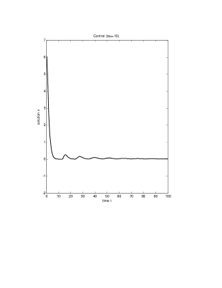
Figure 2: Stabilization with a proportional control for the equation $\ddot{x}(t)+2\dot{x}+x(t-\tau))=\frac{0.8x(t-\tau)}{1+x^{8}(t-\tau)}$ here $\tau=10$ . The left graph illustrates an unstable (oscillating and unbounded) solution while in the right graph, the control $u(t)=x(t-\tau)-x(t)$ produces a stable trajectory.

Consider the nonlinear equation

$$\ddot{x}(t)+a\dot{x}(t)+f(t,x(h(t)))=0$$ (3.10)

which has an equilibrium $x(t)=x^{\ast}$. For stabilization we will use the controller $u=-K[x(t)-x^{\ast}]$, $K>0$ and obtain the equation

$$\ddot{x}(t)+a\dot{x}(t)+f(t,x(h(t)))=-K[x(t)-x^{\ast}].$$ (3.11)

The substitution of $y(t)=x(t)-x^{\ast}$ into equation (3.11) yields

$$\ddot{y}(t)+a\dot{y}(t)+p(t,y(h(t)))=-Ky,$$ (3.12)

where $p(t,v)=f(t,v+x^{\ast})$.

Theorem 3.4.

Suppose $\displaystyle\left|f(t,v+x^{\ast})\right|\leq C|v|$, and at least one of the conditions holds:
a) $C<K\leq a^{2}/4$;    b) $a^{2}/4\leq K<a^{2}/2-C$;    c) $C<a\sqrt{4K-a^{2}}/4$.

Then the equilibrium $x^{\ast}$ of equation (3.10) with the control $u=-K(x(t)-x^{\ast})$ is globally asymptotically stable.

Proof.

Equation (3.12) has the form $\ddot{y}(t)+a\dot{y}(t)+Ky=-p(t,y(h(t))),$ and application of Lemmas 2.1 and 2.2 concludes the proof. ∎

To illustrate application of Theorem 3.4, consider the sunflower equation

$$\ddot{x}(t)+a\dot{x}(t)+A\sin(\omega x(h(t)))=0,~{}~{}a,A,\omega>0.$$ (3.13)

This equation has an infinite number of unstable equilibrium points $x=\frac{(2k+1)\pi}{\omega}$, $k=0,1,\dots$, see Berezansky (arXiv,2014). To stabilize a fixed equilibrium $x^{*}=\frac{(2k+1)\pi}{\omega}$ of equation (3.13), we choose the controller $u=-K\left[x(t)-\frac{(2k+1)\pi}{\omega}\right],K>0$, i.e.

$$\ddot{x}(t)+a\dot{x}(t)+A\sin(\omega x(h(t)))=-K\left[x(t)-\frac{(2k+1)\pi}{\omega}\right].$$ (3.14)

Since $\displaystyle\left|A\sin(\omega v)\right|\leq A\omega|v|$, Theorem 3.4 implies the following result.

Corollary 3.5.

Suppose at least one of the conditions holds:
a) $A\omega<K\leq a^{2}/4$;    b) $a^{2}/4\leq K<a^{2}/2-A\omega$;    c) $A\omega<a\sqrt{4K-a^{2}}/4$.

Then the equilibrium $x^{\ast}=\frac{(2k+1)\pi}{\omega}$ of equation (3.14) is globally asymptotically stable.

4 Summary

The results of the paper can be summarized as follows:

1. For a wide class of nonlinear delay second order equations, we developed stabilizing controls combining the proportional feedback with the proportional derivative feedback.

2. We designed a standard feedback controller which allows to stabilize a second order nonlinear equation with a linear nondelay damping term.

The results are illustrated using nonlinear models with several equilibrium points, for example, modifications of the sunflower equation.

4.1 Acknowledgments

L. Berezansky was partially supported by Israeli Ministry of Absorption, E. Braverman was partially supported by the NSERC DG Research Grant, L. Idels was partially supported by a grant from VIU. The authors are very grateful to the editor and the anonymous referees whose comments significantly contributed to the better presentation of the results of the paper.

References

• Berezansky (2008) L. Berezansky, E. Braverman, A. Domoshnitsky, Stability of the second order delay differential equations with a damping term, Differ. Equ. Dyn. Syst. 16 (2008) 185–205.
• Berezansky (arXiv,2014) L. Berezansky, E. Braverman, L. Idels, Stability tests for second order linear and nonlinear delayed models, arXiv:1403.7554.
• Bielawski (1994) S. Bielawski, D. Derozier, P. Glorieux, Controlling unstable periodic orbits by a delayed continuous feedback, Phys. Rev. E, 49 (2) (1994) R971–R974.
• Boccaletti (2000) S. Boccaletti, C. Grebogi, Y.-C. Lai, H. Mancini, D. Maza, The control of chaos: theory and applications, Phys. Reports, 329 (2000) 103–197.
• Botmart (2012) T. Botmart, P. Niamsup, X. Liu, Synchronization of non-autonomous chaotic systems with time-varying delay via delayed feedback control, Commun. Nonlinear Sci. Numer. Simul. 17 (2012) 1894–1907.
• Cahlon (2004) B. Cahlon, D. Schmidt, Stability criteria for certain second-order delay differential equations with mixed coefficients, J. Comput. Appl. Math. 170 (2004) 79–102.
• Campbell (1995) S. A. Campbell, J. Bélair, T. Ohira, J. Milton, Limit cycles, tori, and complex dynamics in a second-order differential equation with delayed negative feedback, J. Dynam. Diff. Equat. 7 (1995) 213–236.
• Casal (1982) A. Casal, A. Somolinos, Forced oscillations for the sunflower equation, entrainment, Nonlinear Anal. Theor. Meth. Appl., 6 (1982) 397–414.
• Dombovari (2011) Z. Dombovari, D. Barton, R. Wilson, G. Stepan, On the global dynamics of chatter in the orthogonal cutting model, Int. J. Non-Lin. Mech. 46 (2011) 330–338.
• French (2009) M. French, A. Ilchmann, M. Mueller, Robust stabilization by linear output delay feedback, SIAM J. Control Optim. 48 (2009) 2533–2561.
• Freitas (2000) P. Freitas, Delay-induced instabilities in gyroscopic systems, SIAM J. Control Optim. 39 (2000), 196–207.
• Israelson (1967) D. Israelson, A. Johnson, A theory of circumnutations of Helianthus annus, Physiol. Plants 20 (1967), 957–976.
• Johnston (1993) G. Johnston, E. Hunt, Derivative control of the steady state in Chua’s circuit driven in the chaotic region, IEEE Trans. Circuits Systems I Fund. Theory Appl. 40 (1993) 833–835.
• Kim (2013) P. Kim, J. Jung, S. Lee, J. Seok, Stability and bifurcation analysis of chatter vibrations in a nonlinear cylindrical traverse grinding process, J. Sound Vibration, 332 (2013) 3879–3896.
• Kharitonov (2013) V. Kharitonov, Time-delay Systems. Lyapunov Functionals and Matrices, Control Engineering, Birkhäuser/Springer, New York, 2013.
• Konishi (2011) K. Konishi, H. Kokame, N. Hara, Delayed feedback control based on the act-to-wait concept, Nonlinear Dynam. 63 (2011) 513–519.
• Liu (2010) L. Liu, T. Kalmár-Nagy, High-dimensional harmonic balance analysis for second-order delay-differential equations, J. Vib. Control 16 (2010) 1189–1208.
• Lizana (1999) M. Lizana, Global analysis of the sunflower equation with small delay, Nonlinear Anal. Theor. Meth. Appl. 36 (1999) 697–706.
• Ren (2009) J. Ren, Z. Cheng, On high-order delay differential equation. Comput. Math. Appl. 57 (2009) 324–331.
• Reithmeier (2003) E. Reithmeier, G. Leitmann, Robust vibration control of dynamical systems based on the derivative of the state, Arch. Appl. Mech. 72 (2003) 856–864.
• Sipahi (2011) R. Sipahi, S. I. Niculescu, C. T. Abdallah, W. Michiels, K. Gu, Stability and stabilization of systems with time delay: limitations and opportunities, IEEE Control Syst. Mag. 31 (2011) 38–65.
• Somolinos (1978) A. Somolinos, Periodic solution of the sunflower equation $\ddot{x}+(a/r)\dot{x}+(b/r)\sin x(t-r)=0$, Quart. Appl. Math. 4 (1978) 468–478.
• Stepan (2009) G. Stepan, Delay effects in the human sensory system during balancing, Phil. Trans. Roy. Soc. Lond. Ser. A Math. Phys. Eng. Sci. 367 (2009) 1195–1212.
• Stoorvogel (2010) A. A. Stoorvogel, S. Roy, Y. Wan, A. Saberi, A class of neutral-type delay differential equations that are effectively retarded, IEEE Trans. Automat. Control 55 (2010), 435-–440.
• Szalai (2010) R. Szalai, G. Stepan, Period doubling bifurcation and center manifold reduction in a time-periodic and time-delayed model of machining, J. Vib. Control 16 (2010) 1169–1187.
• Rusinek (2014) R. Rusinek et.al, Dynamics of a time delayed Duffing oscillator, Int. J. Non-Lin. Mech. 65 (2014) 98–106.
• Vyhlial (2009) T. Vyhlial, W. Michiels, P. Zitek, P. McGahan, Stability impact of small delays in proportional-derivative state feedback, Control Eng. Practice, 17 (2009) 382–393.
• Wan (2010) M. Wan, W. Zhang, J. Dang, Y. Yang, A unified stability prediction method for milling process with multiple delays, Int. J. Machine Tools Manufacture, 50 (2010) 29–41.
• Wang (2013) X. Wang, A. Saberi, A. A. Stoorvogel, Stabilization of linear system with input saturation and unknown constant delays, Automatica J. IFAC 49 (2013) 3632-–3640.
• Yan (2011) J. Yan, Existence of oscillatory solutions of forced second order delay differential equations, Appl. Math. Lett. 24 (2011) 1455–1460.