Surface code fidelity at finite temperatures

Abstract

We study the dependence of the fidelity of the surface code in the presence of a single finite-temperature massless bosonic environment after a quantum error correction cycle. The three standard types of environment are considered: super-Ohmic, Ohmic, and sub-Ohmic. Our results show that, for regimes relevant to current experiments, quantum error correction works well even in the presence of environment-induced, long-range interqubit interactions. A threshold always exists at finite temperatures, although its temperature dependence is very sensitive to the type of environment. For the super-Ohmic case, the critical coupling constant separating high- from low-fidelity decreases with increasing temperature. For both Ohmic and super-Ohmic cases, the dependence of the critical coupling on temperature is weak. In all cases, the critical coupling is determined by microscopic parameters of the environment. For the sub-Ohmic case, it also depends strongly on the duration of the QEC cycle.

I Introduction

A fundamental challenge to quantum information processing is protection against detrimental effects of the environment Unruh1995 . A milestone in addressing this problem was the development of quantum error correction (QEC) Steane1996 ; CS96 . In fact, it is believed that any practical quantum information processing device will unavoidably contain some sort of QEC Zurek2003 .

The main idea behind active QEC is to encode the information in a region of the system’s Hilbert space known as the logical subspace. This region is chosen to be less vulnerable to the action of the environment. However, during quantum evolution information can leak out of this subspace. This leakage can be diagnosed by measuring some observables in a process known as syndrome extraction. If an error is detected by the syndromes, then a recovery operation is performed. This sequence of actions, extracting the syndrome and a recovery operation, can be called active QEC. It is clear that the QEC protocol demands additional physical and computational resources, thus there is a cost-benefit analysis that must be done. It is believed that there is a particular noise strength below which the benefits of QEC overcome its cost DAMB99 .

Although a large body of work has been devoted to including realistic noise models in the analysis of the QEC efficacy TerhalBurkard2005 ; AGP06 ; AKP2006 ; NB05 ; NMB07 ; NP09b ; NERM10 ; YL15 , there is little discussion on the interplay between the environmental temperature and the dynamics of the system affect the value of threshold for active QEC. An important exception to this is given by Brell and co-workers BBDFP2014 in the context of topological quantum memories that are constantly monitored. In contrast, for passive QEC it is well understood that a finite environmental temperature radically affects the threshold AH06 ; BT09 ; AFH09 ; PhysRevB.90.134302 ; arXiv:1411.6643 . In this paper, we contribute to this theme by considering an environment whose temperature changes due to the interaction with qubits when active QEC is employed. We choose to evaluate the surface code performance against the well-known pure dephasing model when a single logical qubit is in an idle state against super-Ohmic and Ohmic bosonic baths. In order to isolate the effects of finite temperature, we consider a perfect syndrome extraction in a nonerror syndrome evolution and assume all quantum gates and state preparations as flawless. Hence, our thresholds should be regarded as an upper bound to the real QEC threshold. Both analytical results and numerical calculations are presented and we focus on temperatures and time scales relevant to current experimental setups.

Our main result is that, in experimentally relevant regimes, an error threshold always exists, but its dependence on temperature is not universal. While for super-Ohmic environments the critical coupling constant separating high fidelity and low fidelity behavior decreases with increasing temperature, for Ohmic and sub-Ohmic environments the dependence on temperature is weak. For the Ohmic cases, the critical coupling depends primarily on microscopic parameters related to the environment. For the sub-Ohmic case, it depends in addition on the duration of the QEC cycle.

The paper is organized as follows. In Sec. II we provide a brief description of the effect of quantum error correction in the fidelity of a logical qubit coupled to an environment and the evolution is not restricted to uncorrelated errors only. To account for correlations, we consider environments composed of free boson. In Sec. III we develop a finite-temperature formulation for the fidelity of the surface code in the presence of a bosonic environment. The calculation of the fidelity after one QEC cycle is mapped onto the calculation of certain expectation values of a statistical spin model. The analysis that follows in Sec. IV is restricted to a realistic regime where time-correlations (namely, thus developed inside the bosonic light cone) predominate. Three significant cases are studied, namely, super-Ohmic, Ohmic, and sub-Ohmic environments. Both analytical and numerical results are presented. Concluding remarks and a summary are presented in Sec. V. Appendixes with detailed results of calculations and a description of methods employed are provided.

II Quantum error correction in the presence of correlated errors

In order to focus on the effects of correlated errors and the ability of QEC to tame the environmental degrees of freedom, we make two simplifying assumptions. First, we assume that a quantum state can be perfectly prepared. Hence, we consider that the environment and the quantum system are disentangled at the beginning of the evolution. While this assumption could in principle be relaxed, it would result in a much more cumbersome calculation, that would obscure the main effects that we want to discuss. Second, we assume that the environment itself can be initially set to its lowest possible energy state. This choice can easily be relaxed, but would lead to lower threshold values. Even though we allow for the initial state of the environment to be its ground state, we do not assume that it is returned to the ground state at the end of the QEC cycle. Physically, we are considering that the preparation of the initial state and the environment could take a very long time (and we choose the best possible preparation). When the system starts to evolve, the QEC dynamics introduce a finite time scale that limits one’s ability to refrigerate the environment.

In order to clarify the notation and provide a self-contained discussion, we start by giving a brief description of QEC. Following the standard formulation of QEC, see Ref. JP-notes , the unitary evolution of a qubit and its environment in the interaction picture can be described as

$$\hat{U}\left|\psi\right\rangle\left|e_{0}\right\rangle = \hat{I}\left|\psi\right\rangle\left|e_{I}\right\rangle+\hat{X}\left|\psi\right\rangle\left|e_{X}\right\rangle+\hat{Y}\left|\psi\right\rangle\left|e_{Y}\right\rangle$$ (1)

$$+\ \hat{Z}\left|\psi\right\rangle\left|e_{Z}\right\rangle,$$

where $\left|e_{\sigma}\right\rangle$ are environment states (in general non orthogonal and non normalized) and $\hat{I}$, $\hat{X}$, $\hat{Y}$, and $\hat{Z}$ are Pauli operators acting on the qubit. For a system comprised of $n$ qubits, we can straightforwardly define an expansion similar to Eq. (1), namely,

$$\hat{U}\left|\psi\right\rangle\left|e_{0}\right\rangle=\sum_{a}\hat{E}_{a}\left|\psi\right\rangle\left|e_{a}\right\rangle,$$ (2)

where $\hat{E}_{a}\in\left\{\hat{I},\hat{X},\hat{Y},\hat{Z}\right\}^{\otimes n}$.

At the core of any QEC code is the choice of a particular subset ${\cal E}\subseteq\left\{\hat{E}_{a}\right\}$, known as the error set, which the code can correct. The complementary set ${\cal\bar{E}}$ are the uncorrectable errors. It is therefore natural to write the quantum evolution as

$$\hat{U}\left|\psi\right\rangle\left|e_{0}\right\rangle=\sum_{a\in{\cal E}}\hat{E}_{a}\left|\psi\right\rangle\left|e_{a}\right\rangle+\sum_{b\notin{\cal E}}\hat{E}_{b}\left|\psi\right\rangle\left|e_{b}\right\rangle.$$ (3)

The next step in a QEC protocol is the syndrome extraction, where a set of observables corresponding to the projector ${\cal\hat{P}}_{\alpha}$ are measured in order to diagnose the errors and then an appropriate recovery operation $\hat{R}_{\alpha}$ is chosen:

$$\hat{R}_{\alpha}\hat{{\cal P}}_{\alpha}\hat{U}\left|\psi\right\rangle\left|e_{0}\right\rangle=\left|\psi\right\rangle\left|e_{\alpha}\right\rangle+\sum_{b\notin{\cal E}}\hat{R}_{\alpha}\hat{{\cal P}}_{\alpha}\hat{E}_{b}\left|\psi\right\rangle\left|e_{b}\right\rangle.$$ (4)

QEC is in essence a method to steer the quantum evolution of a qubit system through a series of syndrome extractions. Even though QEC in itself is not a perturbative method or description, its cost-benefit analysis is usually done by performing a perturbative expansion in the coupling between the environment and the system. To understand this point, let us consider the fidelity of an initial state after a single QEC step is performed and a syndrome $\alpha$ is detected. The fidelity of the logical state in this case is given by

$${\cal F}_{\alpha}=1-\frac{\left|\left|\sum_{b\notin{\cal E}}\hat{R}_{\alpha}\hat{{\cal P}}_{\alpha}\hat{E}_{b}\left|\psi\right\rangle\left|e_{b}\right\rangle\right|\right|}{\left|\left|\hat{R}_{\alpha}\hat{{\cal P}}_{\alpha}\hat{U}\left|\psi\right\rangle\left|e_{0}\right\rangle\right|\right|},$$ (5)

where, for simplicity, we assumed that the environment states are orthogonal to each other. After the syndrome is extracted only a subset of terms in the Dyson series of the operator $\hat{U}$ is kept. This expansion in the coupling with the environment is used in many calculations of QEC. For instance, in the surface code it is an essential ingredient in the understanding of minimal-weight matching decodings. Hence, if

$$\left|\left|\sum_{b\notin{\cal E}}\hat{R}_{\alpha}\hat{{\cal P}}_{\alpha}\hat{E}_{b}\left|\psi\right\rangle\left|e_{b}\right\rangle\right|\right|\ll\left|\left|\hat{R}_{\alpha}\hat{{\cal P}}_{\alpha}\hat{U}\left|\psi\right\rangle\left|e_{0}\right\rangle\right|\right|,$$ (6)

a high fidelity can be achieved. Thus the choice of ${\cal E}$ and its complement is a choice of the perturbative expansion imposed by the error syndrome $\hat{{\cal P}}_{\alpha}$ extracted for a particular evolution. Clearly, the fidelity can differ from unity due to uncorrectable errors.

Choosing a recovery operation can be difficult in the surface code PNTM2014 . There are strategies for choosing the most likely $\hat{R}_{\alpha}$ for a certain syndrome. However, there is no guarantee that the correct one is chosen. Hence the nonerror syndrome turns out to be of special interest,

$${\cal F}_{0}=1-\frac{\left|\left|\sum_{b\notin{\cal E}}\hat{{\cal P}}_{0}\hat{E}_{b}\left|\psi\right\rangle\left|e_{b}\right\rangle\right|\right|}{\left|\left|\hat{{\cal P}}_{0}\hat{U}\left|\psi\right\rangle\left|e_{0}\right\rangle\right|\right|}.$$ (7)

It requires no recovery operation; thus ${\cal F}_{0}$ corresponds to an intrinsic property of the error model. In this sense, it is expected to provide an upper bound to the fidelity after a QEC cycle with an arbitrary syndromePNTM2014 . We restrict our analysis to the nonerror syndrome case hereafter.

II.1 Correlated and uncorrelated errors

To discuss the concept of a threshold, we need to define a measure of the noise strength. One way to do that is through the fidelity of a single physical qubit,

$${\cal F}_{\mbox{single qubit}} = \left\langle e_{0}\right|\left\langle\psi\right|\hat{U}^{\dagger}\left|\psi\right\rangle\left\langle\psi\right|\hat{U}\left|\psi\right\rangle\left|e_{0}\right\rangle$$ (8)

$$= \left\langle e_{I}|e_{I}\right\rangle$$

$$= 1-p,$$

where $p$ is named the single qubit error probability. Thus, we can rewrite Eq. (8) as

$$p=1-{\cal F_{\mbox{single qubit}}}.$$ (9)

With this quantity, it is possible to define the concept of uncorrelated errors. For instance, for a two-qubit system, the evolution with a nonerror syndrome is said to be uncorrelated if it is possible to write the fidelity resulting from the QEC cycle as

$${\cal F}_{\mbox{two qubits}} = \left\langle e_{0}\right|\left\langle\psi\right|\hat{U}^{\dagger}\left|\psi\right\rangle\left\langle\psi\right|\hat{U}\left|\psi\right\rangle\left|e_{0}\right\rangle,$$ (10)

$$= \left(1-p\right)^{2}.$$

Conversely, when such decomposition of the noise evolution is not possible, the problem is said to contain correlated errors.

Most quantum error threshold discussions in the literature rely on the existence of a single qubit error probability, $p$, and, explicitly or implicitly, rely on uncorrelated error models. Furthermore, we note that the decompositions of Eqs. (1) and (2) are, in general, only valid for a single QEC step. The iteration of the process to the next QEC step demands that the environment and the qubits be again disentangled. Thus, any memory effects between QEC steps are formally excluded in many discussions of the error threshold.

II.2 A microscopic model for correlated errors

A paradigm model in the study of decoherence is the spin-boson model for pure dephasing Weiss1999 ; Breuer2002 . The model consists of free bosons coupled linearly to qubits and whose total $\hat{H}=\hat{H}_{0}+\hat{H}_{{\rm int}}$ contains the free-boson term

$$\hat{H}_{0}=\sum_{{\bf k}}\omega_{{\bf k}}\,\hat{a}_{{\bf k}}^{\dagger}\hat{a}_{{\bf k}}$$ (11)

and the qubit-boson interaction (Breuer2002, , Chap. 4)

$$\hat{H}_{{\rm int}}=\lambda\sum_{{\bf r}}\hat{f}\left({\bf r}\right)\hat{\sigma}_{{\bf r}}^{x},$$ (12)

where $\hat{\sigma}_{{\bf r}}^{x}$ is an $x$ spin operator for the qubit located at site ${\bf r}$, with $\left[\hat{a}_{{\bf k}},\hat{a}_{{\bf q}}^{\dagger}\right]=\delta_{{\bf k},{\bf q}}$, $\omega_{{\bf k}}$ defines the dispersion relation, and

$$\hat{f}\left({\bf r}\right)=\frac{(v/\omega_{0})^{D/2+s}}{L^{D/2}}\sum_{{\bf k}\neq 0}g_{{\bf k}}\,\left(e^{i{\bf k}\cdot{\bf r}}\,\hat{a}_{{\bf k}}^{\dagger}+\mbox{H.c.}\right).$$ (13)

Here, $D$ is the number of spatial dimensions of the bath, $L$ is its linear dimension, $\omega_{0}$ is a characteristic microscopic frequency scale ($\hbar=1$), and $v$ is the bosonic velocity. In Eq. (12), $\lambda$ is the qubit-bath coupling constant, which we separate from the form factor $g_{{\bf k}}$. For convenience, the exponent $s$ is chosen such that $\hat{f}$ is dimensionless and $\lambda$ has units of energy or frequency.

It is straightforward to write the resulting evolution operator in the interaction picture and in normal order,

$$\hat{U}\left(t\right)=\prod_{{\bf k}\neq 0}e^{-\hat{{\cal G}}(t;{\bf k})}\,e^{-i\hat{\alpha}\,\left(t;{\bf k}\right)\,\hat{a}_{{\bf k}}^{\dagger}}\,e^{-i\hat{\alpha}^{*}\,\left(t;{\bf k}\right)\,\hat{a}_{{\bf k}}},$$ (14)

where

$$\hat{\alpha}\left(t;{\bf k}\right)=\frac{\lambda(v/\omega_{0})^{D/2+s}}{L^{D/2}}\sum_{{\bf r}}\frac{g_{{\bf k}}}{\omega_{{\bf k}}}\sin\left(\omega_{k}t/2\right)\hat{\sigma}_{{\bf r},n}^{x}\,e^{i{\bf k}\cdot{\bf r}+i\omega_{{\bf k}}t/2}$$ (15)

and

$$\hat{{\cal G}}\left(t;{\bf k}\right)=\frac{\lambda^{2}}{4L^{D}}(v/\omega_{0})^{D+2s}\int_{0}^{t}dt_{1}\int_{0}^{t}dt_{2}\sum_{{\bf r},{\bf s}}\left|g_{{\bf k}}\right|^{2}e^{-i{\bf k}\cdot\left({\bf r}-{\bf s}\right)-i\omega_{{\bf k}}\left(t_{1}-t_{2}\right)}\,\hat{\sigma}_{{\bf r}}^{x}\,\hat{\sigma}_{{\bf s}}^{x}\,\theta\left(t_{1}-t_{2}\right).$$ (16)

Even though this model does not contain a full set of errors, it is amenable to an exact and explicitly analytical description. Hence it is well suited for exploring the effects of correlations, as well as nonperturbative effects in QEC NB05 .

There are several possible regimes of correlations that can be discussed using this model PNM2013 . They can be classified according to the asymptotic behavior found after tracing out the environment as follows.

1. Super-Ohmic: when some correlation functions of the system have an ultraviolet divergence in the cutoff frequency of the environment. Of course, there are no real divergences on a physical system, with the ultraviolet divergence just signaling that a more accurate description of the small-scale local physics of the qubit is missing from the model.

2. Ohmic: there are log divergences in the ultraviolet and in the infrared correlation functions. This is a more universal behavior, since results depend only on the logarithmic of the ultraviolet and infrared scales of the system.

3. Sub-Ohmic: all correlation functions of the system have a well-defined ultraviolet behavior, but some have infrared divergences.

Both infrared and ultraviolet divergences can be troublesome to QEC, but are amenable by suitable engineering of physical qubits. An ultraviolet divergence signals that the qubit is strongly coupled to the environment at high frequencies. This divergence is controlled by form factors in the qubit design and therefore can be dealt with by appropriate qubit engineering. Conversely, infrared divergences are connected to long-distance correlations. This problem can be addressed by better encoding designs. If we demand only local operations and local communications between physical qubits, an infrared divergence sets a limit on the number of qubits that one can have on the same physical setup.

III QEC with a bath at finite temperature

We assume that the qubits can be prepared in the logical state $\left|\psi\right\rangle$. In order to simplify the calculation and in accordance with Eq. (1), we consider the initial state of the bosonic environment to be the vacuum, $\left|e_{0}\right\rangle=\left|0\right\rangle$. A mixed initial state for the environment could also be considered, but would make the notation and the calculation more complex, obscuring the analysis. Thus, the qubits and the environment are initially in the product state $\left|\psi,0\right\rangle$. In Appendix A we discuss a possible initialization prescription.

After evolving for a time $\Delta$, the density matrix of the combined system becomes

$$\hat{\rho}(\Delta)=\hat{U}(\Delta)\,|\psi,0\rangle\langle\psi,0|\,\hat{U}^{\dagger}(\Delta).$$ (17)

The next step is the syndrome extraction. We assume that the result of this extraction is a nonerror. The occurrence of other types of syndromes would introduce another layer of choices on the decoding procedure, and therefore would potentially further reduce the threshold (see discussion in Ref. PNTM2014 ). Hence we postselect the result of the syndrome in order to write the quantum operation Breuer2002

$$\Phi_{0}\left(\hat{\rho}_{s}\right)=\sum_{m}\hat{\cal P}_{0}\,\hat{\rho}_{s}\,\hat{\cal P}_{0}^{\dagger},$$ (18)

where $\hat{\rho}_{s}$ is a density matrix in the Hilbert space of the qubits and the Kraus operator is the projector

$$\hat{\cal P}_{0}=\left|\bar{\uparrow}\right\rangle\left\langle\bar{\uparrow}\right|+\left|\bar{\downarrow}\right\rangle\left\langle\bar{\downarrow}\right|.$$ (19)

A measurement can be understood as the selection of a pointer basis due to the interaction of the measuring apparatus with another, fast acting, environment Breuer2002 . Hence, during the time that the syndrome is extracted, it is unphysical to regard the total system (bosonic environment and the qubits) as isolated. The extraction of the syndrome bound us to also discuss how the environment would behave during this part of the evolution.

We cannot control the bosonic environment degrees of freedom, but it is possible to place it into contact with an even larger reservoir. This interaction can lead to a dissipative dynamics for the environment that can help in reducing correlations and memory effects. The qubits dynamics cannot affect the environment in any substantial form during the interaction time. Hence, the quantum operation that describes this evolution is

$$\Phi_{\beta}\left(\hat{\rho}_{e}\right)=\sum_{n}\hat{K}_{n}\,\hat{\rho}_{e}\,\hat{K}_{n}^{\dagger},$$ (20)

where $\hat{\rho}_{e}$ is a reduced density matrix in the environment Hilbert space, the Kraus operators are

$$\hat{K}_{n}=\frac{e^{-\beta E_{n}/2}}{\sqrt{Z(\beta)}}\left|n\rangle\langle n\right|,$$ (21)

$E_{n}$ and $|n\rangle$ are the eigenvalues and eigenvectors of $\hat{H}_{0}$, and, finally, the partition function $Z(\beta)=\sum_{n}e^{-\beta E_{n}}$. Since $\sum_{n}\hat{K}^{\dagger}_{n}\,\hat{K}_{n}\leq I$, the result of the quantum operation has to be normalized and the density matrix after the operation is given by

$$\tilde{\rho}_{e}(\beta)=\frac{\Phi_{\beta}\left(\hat{\rho}_{e}\right)}{\mathrm{tr}_{e}\left[\Phi_{\beta}\left(\hat{\rho}_{e}\right)\right]}.$$ (22)

Although it is tempting to associate $\beta$ with the inverse temperature of the larger reservoir, it is straightforward to see that this is an incorrect interpretation. To fully understand the physics of $\hat{K}_{n}$, let us consider a few examples. The first case is the action of $\Phi_{\beta}$ on the “infinity temperature” density matrix, $\hat{\rho}_{e}(\infty)\equiv\sum_{n}\left|n\rangle\langle n\right|$,

$$\tilde{\rho}_{e}(\beta) = \frac{\Phi_{\beta}\left(\hat{\rho}_{e}(\infty)\right)}{\mathrm{tr}_{e}\left[\Phi_{\beta}\left(\hat{\rho}_{e}(\infty)\right)\right]},$$ (23)

$$= \sum_{n}\frac{e^{-\beta E_{n}}}{Z(\beta)}\left|n\rangle\langle n\right|.$$

The bosonic environment is brought from an “infinity” to a $1/\beta$ temperature. Now, if we apply $\Phi_{\beta}$ to Eq. (23), we obtain

$$\frac{\Phi_{\beta}\left(\hat{\rho}_{e}(\beta)\right)}{\mathrm{tr}_{e}\left[\Phi_{\beta}\left(\hat{\rho}_{e}(\beta)\right)\right]}=\sum_{n}\frac{e^{-2\beta E_{n}}}{Z(2\beta)}\left|n\rangle\langle n\right|,$$ (24)

thus corresponding now to an ensemble characterized by a even smaller temperature, $1/(2\beta)$. In general, the operation $\Phi_{e}$ enhances the probabilities of low-energy states in an statistical ensemble instead of equilibrating it at a certain temperature. Therefore, it is possible to call it a refrigeration or cooling mechanism. In Appendix B we discuss a microscopic model that implements this quantum operation.

Combining both quantum operations, $\Phi=\Phi_{\beta}\otimes\Phi_{0}$, produces an action on the Hilbert space of the qubits and the environment. This quantum operation is not normalized, since it is not trace preserving. Thus the correct quantum evolution is given by

$$\tilde{\rho}(\Delta) = \Phi\left(\hat{\rho}(\Delta)\right)$$ (25)

$$= \frac{\sum_{n}\hat{\cal P}_{0}\,\hat{K}_{n}\,\hat{\rho}(\Delta)\,\hat{K}_{n}^{\dagger}\,\hat{\cal P}_{0}}{\text{tr}\left[\sum_{n}\hat{\cal P}_{0}\,\hat{K}_{n}\,\hat{\rho}(\Delta)\,\hat{K}_{n}^{\dagger}\,\hat{\cal P}_{0}\right]}$$ (26)

and the reduced density matrix of the qubits is equal to

$$\tilde{\rho}_{s}\left(\Delta\right)=\text{tr}_{e}\left[\tilde{\rho}(\Delta)\right].$$ (27)

For the qubits, the fidelity between the reduced density matrix at the end of the QEC cycle and the initial density matrix is given by the expression

$${\cal F}=\text{tr}_{s}\left[\tilde{\rho}_{s}\left(\Delta\right)\tilde{\rho}_{s}\left(0\right)\right],$$ (28)

which can be rewritten as

$${\cal F}=\frac{\left\langle 0,\bar{\uparrow}\right|\hat{U}^{\dagger}\left(\Delta\right)\hat{\cal P}_{0}\left|\bar{\uparrow}\right\rangle\left\langle\bar{\uparrow}\right|e^{-\beta\hat{H}_{0}}\,\hat{\cal P}_{0}\,\hat{U}\left(\Delta\right)\left|0,\bar{\uparrow}\right\rangle}{\left\langle 0,\bar{\uparrow}\right|\hat{U}^{\dagger}\left(\Delta\right)\hat{\cal P}_{0}\,e^{-\beta\hat{H}_{0}}\,\hat{U}\left(\Delta\right)\left|0,\bar{\uparrow}\right\rangle},$$ (29)

where we used the relation $\sum_{n}\hat{K}_{n}^{\dagger}\,\hat{K}_{n}=\sum_{n}\frac{e^{-\beta E_{n}}}{Z(\beta)}\left|n\rangle\langle n\right|=e^{-\beta\hat{H}_{0}}/Z(\beta)$.

The best possible scenario for QEC is when, at the end of the cycle, the environment remains at zero temperature. This situation was considered in Refs. NM2013 ; PNM2013 ; PNTM2014 . It corresponds to forcefully setting the environment back to its ground state, hence suppressing some correlations and memory effects. Even in this extreme optimistic case, strong correlations among the qubits can still persist, leading to a nontrivial threshold.

We can further simplify Eq. (29) by considering that

$${\rm tr}\left[|\psi\rangle\langle\psi|\,\hat{\rho}(\Delta)\right] = \frac{e^{-\beta E_{0}}}{Z(\beta)}\,\langle\psi,0|\,\hat{U}^{\dagger}(\Delta;0)\,\hat{{\cal P}}_{0}\,|\psi\rangle$$ (30)

$$\times\langle\psi|\,\hat{{\cal P}}_{0}\,\hat{U}(\Delta;\beta)\,|\psi,0\rangle$$

and

$${\rm tr}\left[\hat{\rho}(\Delta)\right]=\frac{e^{-\beta E_{0}}}{Z(\beta)}\,\langle\psi,0|\hat{U}^{\dagger}(\Delta;0)\,\hat{{\cal P}}_{0}\,\hat{U}(\Delta;\beta)\,|\psi,0\rangle,$$ (31)

where $\hat{U}(\Delta;\beta)=e^{-\beta\hat{H}_{0}}\,\hat{U}(\Delta)\,e^{\beta\hat{H}_{0}}$ and we used $\hat{\cal{P}}_{0}^{2}=\hat{\cal{P}}_{0}$. The end result is that the fidelity can be rewritten as

$${\cal F}_{0}=\frac{\langle\psi,0|\,\hat{U}^{\dagger}(\Delta;0)\,\hat{{\cal P}}_{0}\,|\psi\rangle\langle\psi|\,\hat{{\cal P}}_{0}\,\hat{U}(\Delta;\beta)\,|\psi,0\rangle}{\langle\psi,0|\hat{U}^{\dagger}(\Delta;0)\,\hat{{\cal P}}_{0}\,\hat{U}(\Delta;\beta)\,|\psi,0\rangle}.$$ (32)

When we specialize to the pure dephasing bosonic model, Eq. (12), we obtain a compact expression for the evolution operator

$$\hat{U}(\Delta;\beta)=\prod_{{\bf k}\neq 0}e^{-\hat{{\cal G}}(\Delta;{\bf k})}\,e^{-i\hat{\alpha}(\Delta;{\bf k};\beta)\,\hat{a}_{{\bf k}}^{\dagger}}\,e^{-i\hat{\alpha}^{\ast}(\Delta;{\bf k};\beta)\,\hat{a}_{{\bf k}}},$$ (33)

where

$$\hat{\alpha}(\Delta;{\bf k};\beta) = \frac{\lambda}{L^{D/2}}\left(\frac{v}{\omega_{0}}\right)^{D/2+s}\sum_{{\bf r}}\frac{g_{{\bf k}}}{\omega_{{\bf k}}}\sin\left(\frac{\omega_{k}\Delta}{2}\right)$$ (34)

$$\times \hat{\sigma}_{{\bf r},n}^{x}\,e^{i{\bf k}\cdot{\bf r}+i\omega_{{\bf k}}\left(\frac{\Delta}{2}+i\beta\right)}$$

and

$$\hat{\alpha}^{*}(\Delta;{\bf k};\beta) = \frac{\lambda}{L^{D/2}}\left(\frac{v}{\omega_{0}}\right)^{D/2+s}\sum_{{\bf r}}\frac{g_{{\bf k}}^{*}}{\omega_{{\bf k}}}\sin\left(\frac{\omega_{k}\Delta}{2}\right)$$ (35)

$$\times \hat{\sigma}_{{\bf r},n}^{x}\,e^{-i{\bf k}\cdot{\bf r}-i\omega_{{\bf k}}\left(\frac{\Delta}{2}+i\beta\right)}.$$

III.1 Surface code and the pure dephasing model

The surface code DKLP2002 is regarded as a benchmark among the QEC protocols FSG2009 ; Stephens2014 . It is implemented on a two-dimensional array of qubits, greatly simplifying the design of control and measurement circuits Jones2012 . In addition, all the required interactions between the qubits are spatially local. Finally, it has been estimated that it has a large noise threshold in the absence of correlated errors WFH2011 .

The surface code has the qubits located on the links of a two-dimensional square lattice, as shown in Fig. 1. The quantum code is defined by two sets of operators. The first set corresponds to local operators that define the syndromes that have to be extracted at each QEC step. These are four-body observables,

$$\hat{A}_{\lozenge}=\prod_{{\rm r}\in\lozenge}\hat{\sigma}_{{\rm r}}^{x}$$ (36)

and

$$\hat{B}_{\square}=\prod_{{\rm r}\in\square}\hat{\sigma}_{{\rm r}}^{z},$$ (37)

where $\lozenge$ is a label for the positions of four qubits linked to a vertex of the lattice (“star”) and $\square$ labels the positions of four qubits in a plaquette. To diagnose the evolution of a single logical qubit, all plaquette and star operators have to be measured in order for the syndrome to be extracted.

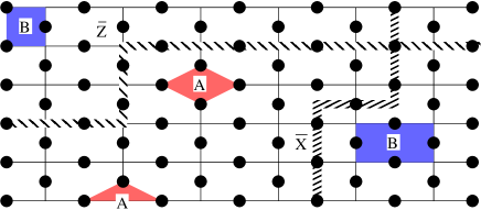
Figure 1: (Color online) Surface code lattice and operators. Physical qubits are located at the edges (black circles). Some star $\hat{A}$ and plaquette $\hat{B}$ operators are indicated, as well, as some realizations of the logical operators $\hat{\bar{X}}$ and $\hat{\bar{Z}}$.

The second set corresponds to two extended operators that act on the logical Hilbert space,

$$\hat{\bar{X}}=\prod_{{\rm r}\in\Gamma}\hat{\sigma}_{{\rm r}}^{x}$$ (38)

and

$$\hat{\bar{Z}}=\prod_{{\rm r}\in\Gamma^{\prime}}\hat{\sigma}_{{\rm r}}^{z},$$ (39)

where $\Gamma$ is any path running from top to bottom of the lattice (dual path) and $\Gamma^{\prime}$ is any path running from left to right of the lattice (primal path), see Fig. 1. Hence, the logical Hilbert space is defined by the basis vectors

$$\left|\bar{\uparrow}\right\rangle=\frac{1}{\sqrt{N_{\lozenge}}}\,\hat{G}\left|F_{z}\right\rangle$$ (40)

and

$$\left|\bar{\downarrow}\right\rangle=\hat{\bar{X}}\left|\bar{\uparrow}\right\rangle,$$ (41)

where $\hat{G}=\prod_{\lozenge}\left(1+\hat{A}_{\lozenge}\right)$, $N_{\lozenge}=2^{n}$ is a normalization constant, $n$ is the number of stars, and $\hat{\sigma}_{{\rm r}}^{z}\left|F_{z}\right\rangle=\left|F_{z}\right\rangle$ for a qubit locate at position ${\rm r}$. The nonerror syndrome projector in the logical Hilbert space can then be written as

$$\hat{{\cal P}}_{0}=\left|\bar{\uparrow}\right\rangle\left\langle\bar{\uparrow}\right|+\hat{\bar{X}}\left|\bar{\uparrow}\right\rangle\left\langle\bar{\uparrow}\right|\hat{\bar{X}}.$$ (42)

In order to investigate the error threshold for a pure dephasing model, it is sufficient to consider that the system is initially prepared in the logical state $\left|\bar{\uparrow}\right\rangle$. Then, the fidelity for a nonerror evolution can be expressed as

$${\cal F}_{0} = \frac{{\cal A}}{{\cal A}+{\cal B}},$$ (43)

where we introduced the amplitudes

$${\cal A}=\left\langle 0\right|\left\langle\bar{\uparrow}\right|\hat{U}^{\dagger}(\Delta,0)\left|\bar{\uparrow}\right\rangle\left\langle\bar{\uparrow}\right|\hat{U}(\Delta;\beta)\left|\bar{\uparrow}\right\rangle\left|0\right\rangle,$$ (44)

and

$${\cal B}=\left\langle 0\right|\left\langle\bar{\uparrow}\right|\hat{U}^{\dagger}(\Delta,0)\,\hat{\bar{X}}\left|\bar{\uparrow}\right\rangle\left\langle\bar{\uparrow}\right|\hat{\bar{X}}\,\hat{U}(\Delta;\beta)\left|\bar{\uparrow}\right\rangle\left|0\right\rangle.$$ (45)

The evolution operators, the star operators, and the logical operators in Eqs. (44) and (45) are diagonal in the $x$ basis of the qubits. Thus it is natural to rewrite the ferromagnetic state as

$$\left|F_{z}\right\rangle=\frac{1}{2^{N/2}}\sum_{\sigma}\left|\sigma\right\rangle,$$ (46)

where $\sigma$ labels the $2^{N}$ eigenstates of the operator $\prod_{{\bf r}}\hat{\sigma}_{{\bf r}}^{x}$, namely, $\prod_{{\bf r}}\hat{\sigma}_{{\rm r}}^{x}\left|\sigma\right\rangle=\pm\left|\sigma\right\rangle$. Using Eq. (46) and assuming $\omega_{{\bf k}}$ is isotropic in ${\bf k}$ footnote , we can write the amplitudes as

$${\cal A}=\sum_{\sigma,\tau}e^{-\lambda^{2}{\cal H}(\Delta;\beta)}\langle\tau|\hat{G}|\tau\rangle\langle\sigma|\hat{G}|\sigma\rangle$$ (47)

and

$${\cal B}=\sum_{\sigma,\tau}e^{-\lambda^{2}{\cal H}\Delta;\beta)}\langle\tau|\hat{\bar{X}}\hat{G}|\tau\rangle\langle\sigma|\hat{\bar{X}}\hat{G}|\sigma\rangle,$$ (48)

where

$${\cal H}(\Delta;\beta) = \frac{N}{2}F(\Delta;0;0)-\frac{1}{2}\,F(\Delta;0;\beta)\sum_{{\bf r}}\sigma_{{\bf r}}\tau_{{\bf r}}+\frac{1}{4}\sum_{{\bf r}\neq{\bf s}}\left[F(\Delta;{\bf r}-{\bf s};0)\left(\tau_{{\bf r}}\tau_{{\bf s}}+\sigma_{{\bf r}}\sigma_{{\bf s}}\right)\right.$$ (49)

$$\left.-\ F(\Delta;{\bf r}-{\bf s};\beta)\left(\sigma_{{\bf r}}\tau_{{\bf s}}+\tau_{{\bf r}}\sigma_{{\bf s}}\right)+i\Phi(\Delta;{\bf r}-{\bf s})\left(\tau_{{\bf s}}-\sigma_{{\bf s}}\right)\left(\tau_{{\bf r}}+\sigma_{{\bf r}}\right)\right],$$

$$F(\Delta;{\bf r};\beta)=\frac{(v/\omega_{0})^{D+2s}}{L^{D}}\sum_{{\bf k}\neq 0}\left|g_{{\bf k}}\right|^{2}e^{-\beta\omega_{{\bf k}}}\left[\frac{1-\cos(\omega_{{\bf k}}\Delta)}{\omega_{{\bf k}}^{\text{2}}}\right]\cos({\bf k}\cdot{\bf r}),$$ (50)

and

$$\Phi(\Delta;{\bf r})=\frac{(v/\omega_{0})^{D+2s}}{L^{D}}\sum_{{\bf k}\neq 0}\left|g_{{\bf k}}\right|^{2}\left[\frac{\omega_{{\bf k}}\Delta-\sin({\bf k}\Delta)}{\omega_{{\bf k}}^{2}}\right]\cos({\bf k}\cdot{\bf r}).$$ (51)

Notice that both functions $F$ and $\Phi$ contain a dependence on interqubit distance, but only the former depends on the environment temperature.

Equations (47) to (51) are quite general. They represent the mapping of the evaluation of the fidelity onto the computation of expectation values of a classical spin system comprising two coupled square-lattice layers and a complex Hamiltonian ${\cal H}$, with $\lambda^{2}$ playing the role of an effective inverse temperature. Notice that the presence of the operator $\hat{G}$ in the matrix elements entering in the expressions for ${\cal A}$ and ${\cal B}$, Eqs. (47) and (48), constrains the sums over the variables $\sigma$ and $\tau$ to configurations with positive plaquettes, namely, to configurations with $\hat{A}_{\diamond}|\sigma\rangle=|\sigma\rangle$ and $\hat{A}_{\diamond}|\tau\rangle=|\tau\rangle$. For configurations containing negative plaquettes, the matrix elements are identically zero.

At this point, in order to carry out a calculation of the fidelity, it is necessary to consider a concrete example. We choose to discuss the well-known pure dephasing decoherence model of Refs. Unruh1995 ; Breuer2002 . Thus we specialize our analysis to situations comprising the following conditions:

1. a two-dimensional ($D=2$) environment;

2. a linear dispersion relation, $\omega_{{\bf k}}=v|{\bf k}|$;

3. a coupling between the qubits and the environmental modes with a power-law behavior, $g_{{\bf k}}=\left|{\bf k}\right|^{s}$;

4. a bosonic ultraviolet cutoff $\Lambda$ for the qubit form factor $g_{{\bf k}}$ smaller than the environment’s natural cutoff.

With these conditions fulfilled and taking the infinite-volume limit, we can rewrite the auxiliary functions in Eqs. (50) and (51) as

$$F(\Delta;{\bf r};\beta) = \frac{1}{\pi}\frac{1}{\omega_{0}^{2}\,(\omega_{0}\Delta)^{2s}}\int_{0}^{\infty}dx\,x^{2s-1}\,J_{0}\left(\frac{\left|{\bf r}\right|x}{v\Delta}\right)$$ (52)

$$\times\ (1-\cos x)\,e^{-\left(\beta+\frac{1}{v\Lambda}\right)x/\Delta},$$

and

$$\Phi(\Delta;{\bf r}) = \frac{1}{\pi}\frac{1}{\omega_{0}^{2}(\omega_{0}\Delta)^{2s}}\int_{0}^{\infty}dx\,x^{2s-1}\,J_{0}\left(\frac{\left|{\bf r}\right|x}{v\Delta}\right)$$ (53)

$$\times\ (x-\sin x)\,e^{-x/(v\Delta\Lambda)},$$

where $J_{0}(z)$ is the zeroth order Bessel function. The parameter $s$ defines the correlation regime of the model: $s>0$ corresponds to a super-Ohmic , $s=0$ to an Ohmic, and $s<0$ to a sub-Ohmic environment.

Following the well-known phenomenology of the single-qubit case, $\beta$ defines the thermal correlation time Breuer2002 . Whenever $\Delta\ll\beta$, the system is in the vacuum regime and systematic corrections can be evaluated in powers of $\Delta/\beta$. The opposite case is the thermal regime, $\beta<\Delta$, which has not been previously studied in the context of the surface code. It is important to note that finite temperature means simply that even though the environment is prepared at zero temperature, the external cooling mechanism cannot suppress the bosonic excitations during the evolution of the system. The functions $F(\Delta;{\bf r};\beta)$ and $\Phi(\Delta;{\bf r})$ in different regimes are presented in Appendix C.

Finally, in order to numerically evaluate the threshold we need to make some additional choices. Guided by the most recent experimental developments of superconducting qubits Chen2014 , which are good candidates for implementing the surface code, we assume a certain range of values for the model’s microscopic parameters.

1. It is reasonable to assume that in a running QEC protocol the environmental temperature for superconducting qubits is of the order of a few millikelvin. Hence, we set $\beta=\frac{\hbar}{k_{B}T}\approx 10^{-9}$ s.

2. It is also reasonable to consider that the QEC period $\Delta$ is of the order of $100$ ns. Therefore, we only consider the thermal regime $\beta\ll\Delta$.

3. Furthermore, the distance between nearest neighbors qubits, $a$, in an superconducting qubit array is likely to be of the order of $10^{-5}$ m.

All the above choices are very reasonable. We note that the thermal regime is likely to be applicable to physical implementations other than the superconducting qubits as well.

The only parameter that is difficult to estimate is the velocity of the bosonic environment. Its value can vary by several orders of magnitude depending on the dominant physical environment. For instance, a typical phonon velocity in solid-state substrates is $v=10^{3}$ m/s; however, electromagnetic fluctuations propagate with $v=10^{8}$ m/s. Roughly, for every power on $10$ in the bosonic velocity, the number of qubits in the time-like cone increases by $10$. Hence, all qubits in an experimental set up would be time-like correlated for the latter case since $v\Delta\gg\left|{\bf r}\right|$. This is likely less so for the phononic environment, but time-like correlations should predominate. Thus, in the following we assume $v\Delta>\left|{\bf r}\right|$.

IV QEC threshold for the pure dephasing model

IV.1 Super-Ohmic environment with $s=1/2$

The $s=1/2$ environment can describe an acoustic phonon bath or an electromagnetic environment Mahan2000 . Using the expressions for the coupling functions defined in Eqs. (50) and (51) presented in Table C of Appendix C, we clearly see that for a super-Ohmic bath $F\left(\Delta;0;0\right)$ diverges with the ultraviolet cutoff and $F\left(\Delta;0;\beta\right)$ diverges with the inverse of the temperature in the thermal regime. Moreover, the ratio of any of other coupling function present in Eq. (49) by one these two diverging couplings tends to zero. Hence, since $F(\Delta,{\bf r},0)$ and $F(\Delta,{\bf r},\beta)$ can be made of the same order in the thermal regime, we can simplify the statistical model and keep only the leading interaction, namely,

$${\cal H}_{\rm super}(\Delta;\beta)=-\,\frac{1}{2}\,F(\Delta;0;\beta)\sum_{{\bf r}}\sigma_{{\bf r}}\,\tau_{{\bf r}}\>,$$ (54)

in order to describe the effect of a super-Ohmic environment on the fidelity. The purely local (yet constrained) spin model defined by the effective two-body interaction of Eq. (54) can be solved exactly by introducing an auxiliary plaquette variable

$$\mu_{{\bf r}-\delta}\,\mu_{{\bf r}+\delta}=\sigma_{{\bf r}}\,\tau_{{\bf r}},$$ (55)

with ${\bf r}\pm\delta$ labeling the plaquettes that share the link where the qubit ${\bf r}$ is located. The statistical sum over the $\mu$ variables in Eqs. (47) and (48) is unconstrained PNTM2014 . Thus the introduction of plaquette spin variables maps the problem onto a standard two-dimensional Ising model with boundary fields. In the thermodynamic limit, $N\rightarrow\infty$, there is a well-known critical coupling Salinas

$$\lambda_{c}=\left[\frac{\ln\left(1+\sqrt{2}\right)}{F\left(\Delta;0;\beta\right)}\right]^{1/2},$$ (56)

separating a region where the fidelity is equal to 1 $(\lambda<\lambda_{c})$ from a region where the fidelity goes to $1/2$ $(\lambda>\lambda_{c})$. We confirm this analytical result performing a standard Monte Carlo simulation, as shown in Fig. 2. The random walk is performed in the mass field variables, while the energy updates are computed using the original spin variables. The numerical simulation clearly indicates the QEC threshold predicted by Eq. (56). We stress that this result is fundamentally different from previous results by the authors NM2013 ; PNTM2014 ; PNM2013 , where the limit $\beta\to\infty$ was taken and therefore the nearest-neighbor coupling in the statistical spin model was the dominant term.

A remarkable feature of Eq. (56) is that the critical coupling for the threshold in a super-Ohmic environment has a square root dependence with the inverse of the temperature but is independent of the QEC time $\Delta$,

$$\lambda_{c}\propto\omega_{0}\,\sqrt{\omega_{0}\,\beta}.$$ (57)

Therefore, for any value of the microscopic coupling with the environment, there will always be a sufficiently low temperature for which the fidelity of the qubit will be 1.

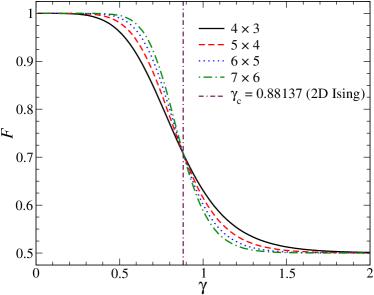
Figure 2: (Color online) Fidelity in the presence of a super-Ohmic environment ($s=1/2$) in the thermal regime for several system sizes. Data obtained by averaging over $10^{9}$ Monte Carlo steps. Here, $\gamma=\lambda^{2}F(\Delta;0;\beta)$. The dashed line marks the phase transition point of an Ising model on a square lattice with nearest-neighbor interactions.

The introduction of the nearest-neighbor coupling to ${\cal H}_{\rm super}$ with the real coupling function $F$, as prescribed by Eq. (49), does not dramatically change these results. However, the addition of the term with the imaginary part $\Phi$ could, in principle, introduce enough oscillations to remove the threshold. Thus we explore numerically the stability of the threshold against the introduction of an imaginary part between nearest neighbors by studying the modified Hamiltonian

$${\cal H}_{\rm super}(\Delta;\beta) = -\,\frac{1}{2}\,F(\Delta;0;\beta)\sum_{{\bf r}}\sigma_{{\bf r}}\,\tau_{{\bf r}}$$

$$+\ \frac{i}{4}\,\Phi(\Delta;d)\sum_{\langle{\bf r},{\bf s}\rangle}\left(\tau_{{\bf s}}-\sigma_{{\bf s}}\right)\left(\tau_{{\bf r}}+\sigma_{{\bf r}}\right),$$

where $d=a/\sqrt{2}$. For time-like correlations and in the thermal regime we expect $\eta\equiv\Phi(\Delta;d)/F(\Delta;0;\beta)\sim\beta/\Delta\ll 1$.

The complex interaction in Eq. (LABEL:eq:Hsuper_imag) prevents the use of the Monte Carlo method. We employ instead Binder’s recursive method to compute the amplitudes ${\cal A}$ and ${\cal B}$ KB72 ; GB90 , as explained in Appendix E. The results for the fidelity are presented in Fig. 3 and show that a shift toward lower thresholds occurs. Hence we conclude that the QEC threshold for the super-Ohmic environment, with $s=1/2$, is mildly robust against small deviations from the asymptotic model defined by Eq. (54). A threshold continues to exists, but it is lowered due to the coherence oscillations caused by the imaginary effective interaction term in the statistical model.

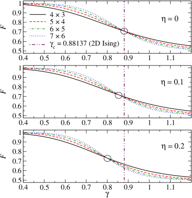
Figure 3: (Color online) Fidelity of the surface code in the presence of a super-Ohmic environment ($s=1/2$) for several system sizes when a small imaginary nearest-neighbor interaction is present; see Eq. (LABEL:eq:Hsuper_imag). Data points obtained using Binder’s method. Here, $\gamma=\lambda^{2}F(\Delta;0;\beta)$ and $\eta=\Phi(\Delta;d)/F(\Delta;0;\beta)$. The dashed line marks the phase transition point of an Ising model in a square lattice with nearest-neighbor interactions. The circle marks the threshold position.

IV.2 Ohmic environment

The Ohmic environment corresponds to $s=0$. Long-range correlations are ubiquitous to this environment, hence it cannot be discussed in the same manner as the super-Ohmic case (see Appendix C).

Some analytical development can be made if we consider the limit where all qubits interact with each other with the same strength (thus taking the logarithmic interaction as a constant): $F\left(\Delta,{\bf r},\beta\right)=\bar{F}$ and $\Phi\left(\Delta,{\bf r}\right)=\bar{\Phi}$, with $\bar{F}\approx\bar{\Phi}\sim 1/\omega_{0}^{2}$. Physically, this corresponds to the distance between the qubits being smaller than the thermal coherence length. In such a simplified model, the Hamiltonian can be rewritten as

$${\cal H}\left(\Delta,\beta\right) = -\,\frac{1}{2}\,\Delta F\sum_{{\bf r}}\sigma_{{\bf r}}\tau_{{\bf r}}+\frac{\bar{F}}{4}\left[\sum_{{\bf r}}\left(\sigma_{{\bf r}}-\tau_{{\bf r}}\right)\right]^{2}$$ (60)

$$+\ i\frac{\bar{\Phi}}{4}\left[\sum_{{\bf r}}\left(\sigma_{{\bf r}}-\tau_{{\bf r}}\right)\right]\left[\sum_{{\bf r}}\left(\sigma_{{\bf r}}+\tau_{{\bf r}}\right)\right]$$

$$= -\,\frac{1}{2}\,\Delta F\sum_{{\bf r}}\sigma_{{\bf r}}\tau_{{\bf r}}+\frac{\bar{F}}{4}(m_{\sigma}-m_{\tau})^{2}$$

$$+\ i\frac{\bar{\Phi}}{4}(m_{\sigma}-m_{\tau})(m_{\sigma}+m_{\tau}),$$

where $\Delta F\equiv F(\Delta;0;\beta)-\bar{F}$, $m_{\sigma}\equiv\sum_{\bf r}\sigma_{\bf r}$ and $m_{\tau}\equiv\sum_{\bf r}\tau_{\bf r}$. It is straightforward to show that, in the absence of QEC, this model causes a reduction of the fidelity proportional to the square of the number of qubits Unruh1995 ; Breuer2002 . The use of QEC changes this scenario quite dramatically. The logical states of the surface code have a finite probability amplitude in most total magnetization sectors $(m_{\sigma},m_{\tau})$. Hence, for nearly every qubit configuration without a logical error one can find another configuration with a logical error and with the same value for the difference $m_{\sigma}-m_{\tau}$. As a consequence, although the effective Hamiltonian in Eq. (60) contains long-range interactions, they do not distinguish between configurations with and without logical errors and the threshold is controlled by the local term proportional to $\Delta F$.

We evaluate numerically the fidelity for the statistical model of Eq. (60) using the Monte Carlo method but disregarding the imaginary part of the interaction. (Unfortunately Binder’s method is no longer practical when interactions go beyond nearest neighbors.) We take $\bar{F}=0.72\Delta F$. The results are presented in Fig. 4 and indicate the existence of a threshold for

$$\lambda_{c}\approx\left[\frac{0.475}{\Delta F\left(\Delta;0;\beta\right)}\right]^{\frac{1}{2}},$$ (61)

thus corresponding to a reduction of about $1/4$ of the super-Ohmic value in Eq. (56).

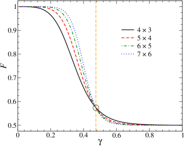
Figure 4: (Color online) Fidelity of the surface code in the presence of an Ohmic bath, as given by the statistical model of Eq. (60), for different lattice sizes. Here, $\gamma=\lambda^{2}\Delta F$, $\bar{\Phi}=0$ and $\bar{F}=0.72\Delta F$. Data obtained by averaging over $10^{9}$ Monte Carlo steps. The location of the transition point, indicated by the crossing point surrounded by a circle, is marked by the dashed line.

The most important difference to the super-Ohmic case is not the numerical value in the coupling constant, but rather the insensitivity to changes in temperature: the threshold depends on temperature only through a logarithm,

$$\lambda_{c}\propto\omega_{0}\left|\ln\left(\frac{\Delta}{\beta}\right)\right|^{-\frac{1}{2}}.$$ (62)

As a result, in practice, only the microscopic frequency scale $\omega_{0}$ determines whether a particular realization of the surface code is above or below the threshold for a given QEC time $\Delta$.

IV.3 Sub-Ohmic environment with $s=-1/2$

A sub-Ohmic environment introduces correlations among very distant qubits. In particular, for the case of $s=-1/2$, as presented in Appendix C, we find that correlations are weakly dependent on qubit-qubit distances and environment temperature. Hence we can revive the analytical discussion used for the Ohmic environment. Considering again the thermal regime and the numerical estimates discussed in Sec. IV.2, namely, $\beta\ll\Delta$ and $v\beta\ll\left|{\bf r}\right|<v\Delta$, we find that $\Delta F\approx\Delta/\omega_{0}$ and temperature independent up to subleading logarithmic corrections. Thus, the critical coupling is controlled by the microscopic characteristic frequency scale $\omega_{0}$ and the QEC time, namely,

$$\lambda_{c}\propto\sqrt{\frac{\omega_{0}}{\Delta}}.$$ (63)

V Discussion and Summary

It is unavoidable that during its quantum evolution a system will get entangled with its environment. This entanglement can be understood as an effective temperature that characterizes the system’s reduced density matrix. To make this point clear, let us consider the simple example of a single qubit interacting with a bosonic environment through the pure bit-flip model Breuer2002 . If the combined system plus environment starts in the pure state $\left|\uparrow\right\rangle_{z}\otimes\left|0\right\rangle$, and we use as the effective Hamiltonian only the site-diagonal term in Eq. (49), the fidelity of this single qubit can be written as

$${\cal F}\left(\Delta,\beta\right)=\frac{1}{1+\bar{M}_{x}},$$ (64)

where $\bar{M}_{x}=\tanh\left[\lambda^{2}\frac{F\left(\Delta;0;\beta\right)}{2}\right]$. The fidelity of this qubit is a smooth function of $\lambda$, going continuously from $1$ to $1/2$.

The $\bar{M}_{x}$ function can be understood as the mean magnetization of a fictitious statistical mechanics problem of a qubit in the presence of a magnetic field, $h=\frac{F\left(\Delta;0;\beta\right)}{2}$, at a temperature $1/\lambda^{2}$. Notice that the actual degrees of freedom of the statistical mechanics problem are not the original qubit variables $\sigma$ and $\tau$, but instead the square of their difference, namely,

$$\mu=1-\frac{1}{2}\left(\sigma-\tau\right)^{2}.$$ (65)

In the spin-boson model literature Leggett:1987:1 , time intervals where $\sigma=\tau$ are called “sojourns”; while for $\sigma=-\tau$ they are called “blips”. Transitions between sojourns and blips correspond to flips of the spin variable $\mu$.

This simple picture is precisely what we generalize in this paper. We consider the fidelity of a single logical qubit coupled to a bosonic environment through a pure bit-flip interaction. After tracing the environment the dynamical problem can once again be mapped onto an effective thermodynamics problem. The remarkable feature of QEC is to transform a crossover into a true phase transition in the limit of a logical qubit with an infinite number of physical qubits. The microscopic parameters that define the transition point yield the intrinsic noise threshold value for the code (which is independent of decoding errors, see discussion in Ref. PNTM2014 ). Ideally it would be preferable to have simultaneously bit-flips and phase flips in an error model; however, this is not fundamental to deduce the existence or not of a threshold.

There are many regimes to consider, but it is very likely that physical realizations of a quantum memory will be in the thermal, $\beta\ll\Delta$, and time-correlated, $\left|{\bf r}\right|<v\Delta$, regimes. For this range of parameters, our main conclusion is that the surface code in a super-Ohmic environment always has a noise threshold and the critical value of the qubit-environment coupling constant goes as $\lambda_{c}\propto\omega_{0}\sqrt{\omega_{0}\beta}$, where $\beta$ is the inverse temperature of the environment at the end of the QEC cycle. Therefore, for the super-Ohmic case, it is always possible to place the system below the noise threshold by reducing the environmental temperature. In contrast, for Ohmic environments, $\lambda_{c}$ is a weak function of temperature and only microscopic parameters play a relevant role in determining whether QEC protects or not the logical qubit state. For sub-Ohmic environments, $\lambda_{c}$ is also approximately temperature independent, but in addition to depending on microscopic scales, it is inversely proportional to the QEC cycle duration.

These results are overall reassuring and indicate that there is no fundamental limitation to the existence of a noise threshold for the surface code in the presence of bosonic environments after a single QEC cycle. We are currently investigating the effects on the fidelity of errors correlated over multiple cycles.

Appendix A Initializing the state

Suppose that the environment is controlled by the Hamiltonian $\hat{H}_{0}$. The Hamiltonian of the combined qubit-environment system is

$$\hat{H}=\hat{H}_{0}+\sum_{{\bf r}}\left[\hat{f}\left({\bf r}\right)\hat{\sigma}_{{\bf r}}^{z}-h\,\hat{\sigma}_{{\bf r}}^{z}\right],$$ (66)

where $\hat{f}\left({\bf r}\right)$ represents the interaction between the qubit at position ${\bf r}$ and the environment and $h$ is an external field. The density matrix of the system at thermal equilibrium reads

$$\hat{\rho}\left(\beta,h\right)=\frac{e^{-\beta\hat{H}}}{Z},$$ (67)

where $Z$ is the partition function, $Z=\text{tr}\left[e^{-\beta\hat{H}}\right]$.

The Hamiltonian in Eq. (66) is diagonal in the qubit space. Assume that $h$ is large and the qubits are frozen in the $+z$ direction. Then,

$$\hat{\rho}\left(\beta,h\to\infty\right)=\frac{e^{-\beta\left[\sum_{k}\omega_{k}\,\hat{a}_{k}^{\dagger}\,\hat{a}_{k}+\lambda\sum_{n}\hat{f}\left(n\right)\right]}}{Z}\otimes\left|F\rangle\langle F\right|,$$ (68)

where $\left|F\right>$ is the ferromagnetic $z$ state of the qubits. Using Eq. (11), it is natural to define $\hat{b}_{k}=\hat{a}_{k}+\alpha_{k}/\omega_{k}$ in order to rewrite the bosonic Hamiltonian as

$$\omega_{k}\,\hat{b}_{k}^{\dagger}\,\hat{b}_{k}=\omega_{k}\,\hat{a}_{k}^{\dagger}\,\hat{a}_{k}+\alpha_{k}\,\hat{a}_{k}^{\dagger}+\alpha_{k}^{*}\,\hat{a}_{k}+\frac{\left|\alpha_{k}\right|^{2}}{\omega_{k}}$$ (69)

and the density matrix as

$$\hat{\rho}\left(\beta,h\to\infty\right)=\frac{e^{-\beta\left[\sum_{k}\omega_{k}\,\hat{b}_{k}^{\dagger}\,\hat{b}_{k}\right]}}{\bar{Z}}\otimes\left(\left|F\rangle\langle F\right|\right),$$ (70)

where $\bar{Z}$ is the partition function for the new $\hat{b}_{k}$ bosons. Raking the temperature to zero ($\beta\to\infty$), we arrive at

$$\hat{\rho}\left(\beta\to\infty,h\to\infty\right)=\left|\bar{0}\rangle\langle\bar{0}\right|\otimes\left|F\rangle\langle F\right|,$$ (71)

where $|\bar{0}\rangle$ is the ground state of the $\hat{b}_{k}$ bosons. This ground state is a coherent state of the original $\hat{a}_{k}$ bosons,

$$\hat{a}_{k}|\bar{0}\rangle=-\lambda\left|{\bf k}\right|^{s-1}\frac{\sum_{n}e^{-i{\bf k}\cdot{\bf r}_{n}}}{vL^{D/2}}\,|\bar{0}\rangle.$$ (72)

However, if the qubits do not form a dense set with respect to the bosonic environment, then, in the limit $L\to\infty$,

$$|\bar{0}\rangle=|0\rangle,$$ (73)

and we obtain the state

$$\hat{\rho}\left(\beta\to\infty,h\to\infty\right)=|0\rangle\langle 0|\otimes|F\rangle\langle F|.$$ (74)

Finally, assuming the ability of instantaneous (faster than the environment inverse cutoff) and flawless gates, the initial state can be prepared as

$$\hat{\rho}_{0} = |0\rangle\langle 0|\otimes G\,|F\rangle\langle F|G$$ (75)

$$= |0\rangle\langle 0|\otimes\left|\bar{\uparrow}\right\rangle\left\langle\bar{\uparrow}\right|.$$ (76)

Appendix B Microscopic Cooling Mechanism

A microscopic description of the cooling process of the free bosonic environment coupled to the qubits proceeds as follows. The relation of the bosonic environment and an external reservoir can be described by the usual damped harmonic oscillator master equation Breuer2002 . For an illustrative example of this microscopic description, consider qubits inside an electromagnetic cavity. The modes inside the cavity constitute the correlated environment. However, there are electromagnetic modes outside the cavity as well. These external modes can damp the modes inside the cavity.

For a given bosonic mode, the master equation, after the usual Born-Markov approximations, is given by

$$\frac{d}{dt}\hat{\rho}_{{\bf k}} = -i\omega_{{\bf k}}\left[\hat{a}_{{\bf k}}^{\dagger}\,\hat{a}_{{\bf k}},\hat{\rho}_{{\bf k}}\right]$$ (77)

$$+\ \gamma_{\bf k}\left(N_{\bf k}+1\right)\left(\hat{a}_{{\bf k}}\,\hat{\rho}_{{\bf k}}\,\hat{a}_{{\bf k}}^{\dagger}-\frac{1}{2}\hat{a}_{{\bf k}}^{\dagger}\,\hat{a}_{{\bf k}}\,\hat{\rho}_{{\bf k}}-\frac{1}{2}\hat{\rho}_{{\bf k}}\,\hat{a}_{{\bf k}}^{\dagger}\,\hat{a}_{{\bf k}}\right)$$

$$+\ \gamma_{\bf k}N_{\bf k}\left(\hat{a}_{{\bf k}}^{\dagger}\,\hat{\rho}_{{\bf k}}\,\hat{a}_{{\bf k}}-\frac{1}{2}\hat{a}_{{\bf k}}\,\hat{a}_{{\bf k}}^{\dagger}\,\hat{\rho}_{{\bf k}}-\frac{1}{2}\hat{\rho}_{{\bf k}}\,\hat{a}_{{\bf k}}\,\hat{a}_{{\bf k}}^{\dagger}\right),$$

where $N_{\bf k}=\left[\exp\left(\tilde{\beta}\omega_{{\bf k}}\right)-1\right]^{-1}$, $\gamma_{\bf k}$ is the damping rate, and we defined the inverse temperature $\tilde{\beta}=1/\tilde{T}$ ($k_{B}=1$). In order to maximize the cooling and be compatible with the initial state chosen for the bosonic environment (see Appendix A), the external reservoir should be at its lowest possible temperature, $\tilde{T}=0$.

If we evoke the usual assumption that decoherence is much faster than dissipation, we can focus on solving the master equation for the populations, known as Pauli master equation. For $\tilde{T}=0$ it is simply

$$\frac{d}{dt}P_{\bf k}(n,t)=\gamma_{\bf k}\left[(n+1)P_{\bf k}(n+1,t)-nP_{\bf k}(n,t)\right],$$ (78)

where $P_{\bf k}(n,t)=\langle{\bf k};n|\hat{\rho}_{\omega_{{\bf k}}}(t)|{\bf k};n\rangle$ and $n$ denotes the number of ${\bf k}$ modes Breuer2002 .

These coupled differential equations are easily solvable if we consider that the original populations are only sparsely nonzero, i.e., if $P_{\bf k}(n,0)\neq 0$, then $P_{\bf k}(n\pm 1,0)=0$. Considering that syndrome extraction takes a time $t=\epsilon$, the initial population of mode ${\bf k}$ is reduced to

$$P_{\bf k}(n,\epsilon)=e^{-\gamma_{\bf k}\,n\,\epsilon}\,P_{\bf k}(n,0).$$ (79)

It is also reasonable to assume that the damping rate is a function of the energy of the bosonic mode. A simple choice is to make it a linear relation,

$$\gamma_{\bf k}\,n\,\epsilon=\langle n|\beta\,\omega_{\bf k}\,\hat{a}^{\dagger}_{\bf k}\,\hat{a}_{\bf k}|n\rangle.$$ (80)

This corresponds physically to having higher frequencies coupled more strongly to the external reservoir than lower ones. Therefore, a given environmental mode with initial density matrix

$$\hat{\rho}_{\bf k}(0)=\sum_{n,m}w_{n,m}|{\bf k};n\rangle\langle{\bf k};m|,$$ (81)

evolves towards

$$\hat{\rho}_{{\bf k}}(\epsilon)=\sum_{n}w_{n,n}\,e^{-\beta\,\omega_{\bf k}\,\hat{a}^{\dagger}_{\bf k}\,\hat{a}_{\bf k}}|{\bf k};n\rangle\langle{\bf k};n|.$$ (82)

These considerations hold for all environmental modes ${\bf k}$. Finally, if we assume that decoherence would quickly destroy the coherences between different environmental modes, we find that the initial density matrix of the environment,

$$\hat{\rho}_{e}(0)=\sum_{i,j}w_{i,j}\,|i\rangle\langle j|,$$ (83)

evolves towards the density matrix

$$\hat{\rho}_{e}(\epsilon)=\sum_{i}w_{i,i}\,e^{-\beta\hat{H}_{0}}|i\rangle\langle i|.$$ (84)

That corresponds to the quantum operation $\Phi_{\beta}\left(\hat{\rho}_{e}(0)\right)$, where $\beta$ is defined as a function of the damping rates of the environment, Eq. (80). The particular case of $\beta=0$ corresponds to having no damping, hence describing a situation where the environment has a unitary evolution during the syndrome extraction.

Appendix C Coupling constants for some environments

The evaluation of Eqs. (50) and (51) is a straightforward but long task. Closed forms can only be found for special values of $s$. Here we present results for some representative cases and for different environments. As discussed in the main text, the inverse temperature $\beta$ defines the thermal coherence time, creating two limiting regimes. For the quantum vacuum regime we can assume $\Delta/\beta\ll 1$ to evaluate the integrals. Conversely, for the thermal regime we can assume that $\beta/\Delta\ll 1$. Finally, during the evaluation of Eqs. (50) and (51) it is assumed that all distances $\left|{\bf r}\right|$ are much larger than $\mbox{max}\{v\beta,\Lambda^{-1}\}$. The results are presented in Table C.

	super-Ohmic ($s=\frac{1}{2})$	Ohmic ($s=0)$	sub-Ohmic ($s=-\frac{1}{2})$

& $\frac{\Delta}{2\omega_{0}}$ $\Phi(\Delta;{\bf r}\neq 0)$ $\frac{v}{\pi\omega_{0}^{3}}\frac{\theta(v\Delta-\left|{\bf r}\right|)}{\sqrt{v^{2}\Delta^{2}-\left|{\bf r}\right|^{2}}}$ $\frac{1}{\pi\omega_{0}^{2}}\left[\frac{\pi}{2}\theta(v\Delta-\left|{\bf r}\right|)+\right.$ $\left.\arcsin\left(\frac{v\Delta}{\left|{\bf r}\right|}\right)\theta(\left|{\bf r}\right|-v\Delta)\right]$ $\frac{\Delta}{\pi\omega_{0}}\ln\left[\sqrt{\left(\frac{v\Delta}{{\bf r}}\right)^{2}-1}+\frac{v\Delta}{{\bf r}}\right.$ $\left.-\sqrt{1-\left(\frac{{\bf r}}{v\Delta}\right)^{2}}\right]\theta\left(v\Delta-{\bf r}\right)$ $F_{\mbox{thermal}}(\Delta;0;\beta)$ $\frac{1}{\pi\omega_{0}^{3}\beta}$ $\frac{1}{\pi}\frac{1}{\omega_{0}^{2}}\ln\left(\frac{\Delta}{\beta}\right)$ $\frac{\Delta}{\pi\omega_{0}}\left(\frac{\pi}{2}+\frac{\beta}{\Delta}\ln\frac{\beta}{\Delta}\right)$ $F_{\mbox{thermal}}(\Delta;{\bf r}\neq 0;\beta)$ $\frac{v}{\pi\omega_{0}^{3}}\left[\frac{1}{\left|{\bf r}\right|}-\frac{\theta(\left|{\bf r}\right|-v\Delta)}{\sqrt{\left|{\bf r}\right|^{2}-v^{2}\Delta^{2}}}\right]$ $\frac{1}{\pi\omega_{0}^{2}}\left[\mbox{arccosh}\left(\frac{v\Delta}{\left|{\bf r}\right|}\right)\theta(v\Delta-\left|{\bf r}\right|)\right.$ $\left.+\frac{v\beta}{\sqrt{\left|{\bf r}\right|^{2}-\left(v\Delta\right)^{2}}}\theta\left(\left|{\bf r}\right|-v\Delta\right)-\frac{v\beta}{\left|{\bf r}\right|}\right]$ $\frac{\Delta}{\pi\omega_{0}}\left\{\left[\left(\frac{\pi}{2}-\frac{\left|{\bf r}\right|}{v\Delta}\right)+\right.\right.$ $\left.\mbox{$\frac{\beta}{\Delta}$arccosh}\left(\frac{v\Delta}{\left|{\bf r}\right|}\right)\right]\theta(v\Delta-\left|{\bf r}\right|)$ +$\left[\arcsin\frac{v\Delta}{\left|{\bf r}\right|}+\right.$ $\left.\left.\sqrt{\left(\frac{\left|{\bf r}\right|}{v\Delta}\right)^{2}-1}-\frac{\left|{\bf r}\right|}{v\Delta}\right]\theta(\left|{\bf r}\right|-v\Delta)\right\}$

Table 1: Coupling constants for different noise regimes.

Appendix D Mass field formulation

One of the main difficulties in evaluating Eqs. (47) and (48) numerically is to enforce the positive star constraints. An efficient method to enforce the constraint is to introduce auxiliary plaquette variables, the so-called mass fields PNTM2014 , for the bulk qubits in the surface code,

$$\sigma_{\mathbf{r}}=\mu_{\mathbf{m}}\mu_{\mathbf{n}},$$ (85)

and

$$\tau_{\mathbf{r}}=\nu_{\mathbf{m}}\nu_{\mathbf{n}},$$ (86)

where $\mathbf{m}$ and $\mathbf{n}$ denote the plaquettes that share the edge where the spin site $\mathbf{r}$ is located (see Fig. 5). For qubits on the top and bottom boundaries, we follow the discussion in Ref. NM2013 and use instead

$$\sigma_{\mathbf{r}}=\mu_{\mathbf{m}}\alpha_{t}$$ (87)

or

$$\sigma_{\mathbf{r}}=\mu_{\mathbf{m}}\alpha_{b}$$ (88)

and

$$\tau_{\mathbf{r}}=\nu_{\mathbf{m}}\beta_{t}$$ (89)

or

$$\tau_{\mathbf{r}}=\nu_{\mathbf{m}}\beta_{b},$$ (90)

with $\alpha_{t},\alpha_{b},\beta_{t},\beta_{b}=\pm 1$.

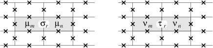
Figure 5: Mass field variable composition.

The introduction of mass fields automatically enforce positive stars: $\langle\mu|\hat{G}|\mu\rangle=\langle\nu|\hat{G}|\nu\rangle=1$ for all $\mu$ and $\nu$. In addition,

$$\langle\sigma|\hat{X}\hat{G}|\sigma\rangle = \alpha_{t}\alpha_{b}$$ (91)

and

$$\langle\tau|\hat{X}\hat{G}|\tau\rangle = \beta_{t}\beta_{b}.$$ (92)

In the mass field variables it is evident that the effective energy of the qubit configurations that contribute to the amplitudes in Eqs. (47) and (48) obeys some symmetry properties. For instance, time-reversal symmetry still holds,

$$E(\mu,\nu;\alpha,\beta)=E(-\mu,-\nu;-\alpha,-\beta),$$ (93)

as well as complex conjugation through the exchange of mass-field and boundary-field variables,

$$E(\mu,\nu;\alpha,\beta)=[E(\nu,\mu;\beta,\alpha)]^{\ast}.$$ (94)

In addition to automatically enforcing the positive star constraints, the mass fields are also very useful to deal with on-site and nearest-neighbor interactions in the original qubits. If we restrict ourselves to this particular case of nearest neighbor, and define

$$J=\frac{F\left(\Delta,a,\beta\right)+i\Phi\left(\Delta,a\right)}{F\left(\Delta,0,\beta\right)},$$ (95)

we find that the energy can be written as

$$E(\mu,\nu;\alpha,\beta) =E_{\mathrm{bulk}}(\mu,\nu)+E_{\mathrm{top}}(\mu,\nu;\alpha_{t},\beta_{t})+E_{\mathrm{bottom}}(\mu,\nu;\alpha_{b},\beta_{b})$$

where

$$E_{\mathrm{bulk}}(\mu,\nu)=\frac{1}{2}\left[N-\sum_{\langle\mathbf{m},\mathbf{n}\rangle}\mu_{\mathbf{m}}\mu_{\mathbf{n}}\nu_{\mathbf{m}}\nu_{\mathbf{n}}\right]+J^{\ast}\sum_{\langle\langle\mathbf{m},\mathbf{n}\rangle\rangle}\mu_{\mathbf{m}}\mu_{\mathbf{n}}+J\sum_{\langle\langle\mathbf{m},\mathbf{n}\rangle\rangle}\nu_{\mathbf{m}}\nu_{\mathbf{n}}-\mathrm{Re}\{J\}\left[\sum_{\langle\mathbf{m},\mathbf{n},\mathbf{m}^{\prime}\rangle}\mu_{\mathbf{m}}\mu_{\mathbf{n}}\nu_{\mathbf{n}}\nu_{\mathbf{m}^{\prime}}\right],$$ (96)

$$E_{\mathrm{top}}(\mu,\nu;\alpha_{t},\beta_{t}) = -\frac{1}{2}\left[\alpha_{t}\beta_{t}\sum_{\mathbf{m}\in y=N_{y}}\mu_{\mathbf{m}}\nu_{\mathbf{m}}\right]+J^{\ast}\alpha_{t}\left[\sum_{\mathbf{m}\in y=N_{y},2\leq x\leq N_{x}-1}\mu_{\mathbf{m}}+\frac{1}{2}(\mu_{1,N_{y}}+\mu_{N_{x},N_{y}})\right]$$ (97)

$$+\ J\beta_{t}\left[\sum_{\mathbf{m}\in y=N_{y},2\leq x\leq N_{x}-1}\nu_{\mathbf{m}}+\frac{1}{2}(\nu_{1,N_{y}}+\nu_{N_{x},N_{y}})\right]$$

$$-\ \mathrm{Re}\{J\}\left[\alpha_{t}\sum_{\langle\mathbf{m},\mathbf{n}\rangle\in y=N_{y}}\nu_{\mathbf{m}}\nu_{\mathbf{n}}\mu_{\mathbf{n}}+\beta_{t}\sum_{\langle\mathbf{m},\mathbf{n}\rangle\in y=N_{y}}\mu_{\mathbf{m}}\mu_{\mathbf{n}}\nu_{\mathbf{n}}\right],$$

and

$$E_{\mathrm{bottom}}(\mu,\nu;\alpha_{b},\beta_{b}) = -\frac{1}{2}\left[\alpha_{b}\beta_{b}\sum_{\mathbf{m}\in y=1}\mu_{\mathbf{m}}\nu_{\mathbf{m}}\right]+J^{\ast}\alpha_{b}\left[\sum_{\mathbf{m}\in y=1,2\leq x\leq N_{x}-1}\mu_{\mathbf{m}}+\frac{1}{2}(\mu_{1,1}+\mu_{N_{x},1})\right]$$ (98)

$$+\ J\beta_{b}\left[\sum_{\mathbf{m}\in y=1,2\leq x\leq N_{x}-1}\nu_{\mathbf{m}}+\frac{1}{2}(\nu_{1,1}+\nu_{N_{x},1})\right]$$

$$-\ \mathrm{Re}\{J\}\left[\alpha_{b}\sum_{\langle\mathbf{m},\mathbf{n}\rangle\in y=1}\nu_{\mathbf{m}}\nu_{\mathbf{n}}\mu_{\mathbf{n}}+\beta_{b}\sum_{\langle\mathbf{m},\mathbf{n}\rangle\in y=1}\mu_{\mathbf{m}}\mu_{\mathbf{n}}\nu_{\mathbf{n}}\right],$$

where $N_{x}$ and $N_{y}$ indicate the horizontal and vertical number of plaquettes in the surface code lattice.

There are two features that complicate any numerical calculation: the appearance of three-body interactions and the next-to-nearest neighbor interactions. Both of these features make any recursive computation very difficult and any Monte-Carlo simulation less efficient (if at all possible, due to the presence of an imaginary coupling).

In terms of mass fields and boundary fields, the targets of the calculation are the quantities

$${\cal B}=\frac{1}{Z}\sum_{\alpha_{t},\alpha_{b}=\pm 1}\sum_{\beta_{t},\beta_{b}=\pm 1}\sum_{\{\mu\}}\sum_{\{\nu\}}e^{-\xi E(\mu,\nu;\alpha,\beta)}\alpha_{t}\alpha_{b}\beta_{t}\beta_{b}$$ (99)

and

$$Z=\sum_{\alpha_{t},\alpha_{b}=\pm 1}\sum_{\beta_{t},\beta_{b}=\pm 1}\sum_{\{\mu\}}\sum_{\{\nu\}}e^{-\xi E(\mu,\nu;\alpha,\beta)},$$ (100)

where $\xi\equiv\lambda^{2}F\left(\Delta,0,\beta\right)$ is a fictitious temperature. It is straightforward to prove that $Z$ and ${\cal B}$ are real quantities. Furthermore, from $Z\left(\gamma\right)$ we can compute the expectation value of the effective energy and corresponding heat capacity,

$$E=-\frac{d\ln Z}{d\xi},$$ (101)

and

$$C=-\xi^{2}\frac{dE}{d\xi}.$$ (102)

Using the auxiliary function

$$c(\alpha,\beta) \equiv \sum_{\{\mu\}}\sum_{\{\nu\}}e^{-\xi E(\mu,\nu;\alpha,\beta)},$$ (103)

we can write

$$Z = 2\left[c(+,+,+,+)+2c(+,+,+,-)\right.$$ (104)

$$+\ 2c(+,-,+,+)+c(+,+,-,-)$$

$$+\ \left.c(+,-,+,-)+c(+,-,-,+)\right]$$

and

$${\cal B} = \frac{2}{Z}\left[c(+,+,+,+)-2c(+,+,+,-)\right.$$ (105)

$$-\ 2c(+,-,+,+)+c(+,+,-,-)$$

$$+\ \left.c(+,-,+,-)+c(+,-,-,+)\right],$$

where we used the time-reversal symmetry of $E(\mu,\nu;\alpha,\beta)$ to reduce the number of terms.

Appendix E Binder’s recursive method for the surface code with nearest-neighbors interactions

We can extend Binder’s recursive method KB72 ; GB90 for computing the partition function of the Ising model in a two-dimensional square lattice with nearest-neighbor interactions to the effective statistical model of Eq. (49). Two modifications are necessary: (i) to consider two spins per site and (ii) to introduce auxiliary variables in the recursive steps.

Suppose we start with a square lattice of dimensions $N_{x}\times N_{y}$ ($N_{x}$ columns and $N_{y}$ rows). To each lattice site on a row we associate two binary numbers $(s_{x},r_{x})$, with $s_{x}=0,1$, $r_{x}=0,1$ and $x=1,\ldots,N_{x}$. We can then index the state of the spins in a lattice row by two integers $(\mathbf{s},\mathbf{r})$, where

$$\mathbf{s}=s_{N}\times 2^{N-1}+s_{N-1}\times 2^{N-2}+\ldots+s_{2}\times 2^{1}+s_{1}\times 2^{0}$$ (106)

and

$$\mathbf{r}=r_{N}\times 2^{N-1}+r_{N-1}\times 2^{N-2}+\ldots+r_{2}\times 2^{1}+r_{1}\times 2^{0}.$$ (107)

The numbers $\mathbf{s}$ and $\mathbf{r}$ are related to the mass field variables $\mu$ and $\nu$ by

$$\mu_{x,y} = 2s_{x}-1$$ (108)

$$\nu_{x,y} = 2r_{x}-1,$$ (109)

where $x=1,\ldots,N$.

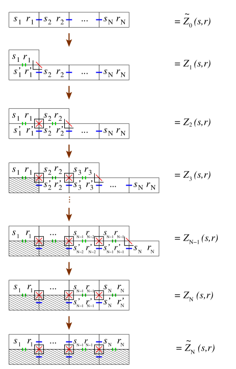
Figure 6: (Color online) Thick horizontal lines represent two-body nearest-neighbor horizontal interactions. Short thick double vertical lines represent two-body nearest-neighbor vertical interactions. Diagonal thin lines represent two-body next-to-nearest neighbor interactions. L-shaped lines and squares represent three-body interactions.

Let $Z_{0}(\mathbf{s},\mathbf{r})$ denote the partition function term containing the first (bottom) row of the lattice when only nearest-neighbor interactions within that row are taken into account. From this partial partition function we can build the full partition function of the entire lattice (see Fig. 6) with the following recursive protocol.

1. Find $Z_{0}(\mathbf{s},\mathbf{r})$ for the first (bottom) row.

2. Incorporate boundary fields (the dependence on boundary fields is left implicit hereafter):

   $$\tilde{Z}_{0}(\mathbf{s},\mathbf{r})=Z_{0}(\mathbf{s},\mathbf{r})\kappa(\alpha_{b},\beta_{b},\mathbf{s},\mathbf{r}).$$ (110)

3. Evaluate $Z_{1}(\mathbf{s},\mathbf{r};s_{1}^{\prime},r_{1}^{\prime})$ at the second row, first site:

   $$Z_{1}(\mathbf{s},\mathbf{r};s_{1}^{\prime},r_{1}^{\prime})=\eta(s_{1},r_{1};s_{2},r_{2},s_{1}^{\prime},r_{1}^{\prime})\tilde{Z}_{0}(\mathbf{s}^{\prime},\mathbf{r}^{\prime}),$$ (111)

   where $\mathbf{s}^{\prime}=\mathbf{s}+s_{1}^{\prime}-s_{1}$ and $\mathbf{r}^{\prime}=\mathbf{r}+r_{1}^{\prime}-r_{1}$.

4. Evaluate $Z_{2}(\mathbf{s},\mathbf{r};s_{2}^{\prime},r_{2}^{\prime})$ at the second row, second site:

   $$Z_{2}(\mathbf{s},\mathbf{r};s_{2}^{\prime},r_{2}^{\prime}) = \eta(s_{2},r_{2};s_{3},r_{3},s_{2}^{\prime},r_{2}^{\prime})$$ (112)

   $$\times\sum_{s_{1}^{\prime},r_{1}^{\prime}}\lambda(s_{1},r_{1};s_{2},r_{2};s_{1}^{\prime},r_{1}^{\prime};s_{2}^{\prime},r_{2}^{\prime})$$

   $$\times\ Z_{1}(\mathbf{s}^{\prime},\mathbf{r}^{\prime};s_{1}^{\prime},r_{1}^{\prime}),$$

   where $\mathbf{s}^{\prime}=\mathbf{s}+2(s_{2}^{\prime}-s_{2})$ and $\mathbf{r}^{\prime}=\mathbf{r}+2(r_{2}^{\prime}-r_{2})$. Update $Z_{1}=Z_{2}$.

5. Evaluate $Z_{k}(\mathbf{s},\mathbf{r};s_{k}^{\prime},r_{k};)$ at the second row, $k$-th site ($2<k\leq N_{x}-1$):

   $$Z_{2}(\mathbf{s},\mathbf{r};s_{k}^{\prime},r_{k}^{\prime}) = \eta(s_{k},r_{k};s_{k+1},r_{k+1},s_{k}^{\prime},r_{k}^{\prime})\sum_{s_{k-1}^{\prime},r_{k-1}^{\prime}}$$ (113)

   $$\lambda(s_{k-1},r_{k-1};s_{k},r_{k};s_{k-1}^{\prime},r_{k-1}^{\prime};s_{k}^{\prime},r_{k}^{\prime})$$

   $$\times\ Z_{1}(\mathbf{s}^{\prime},\mathbf{r}^{\prime};s_{k-1}^{\prime},r_{k-1}^{\prime}),$$

   where $\mathbf{s}^{\prime}=\mathbf{s}+2^{k-1}(s_{k}^{\prime}-s_{k})$ and $\mathbf{r}^{\prime}=\mathbf{r}+2^{k-1}(r_{k}^{\prime}-r_{k})$. Update $Z_{1}=Z_{2}$.

6. Evaluate $Z_{N_{x}}(\mathbf{s},\mathbf{r})$ at the second row, $N_{x}$-th site:

   $$Z_{2}(\mathbf{s},\mathbf{r}) = \sum_{s_{N_{x}}^{\prime},r_{N_{x}}^{\prime}}\gamma(s_{N_{x}},r_{N_{x}};s_{N_{x}}^{\prime},r_{N_{x}}^{\prime})\sum_{s_{N_{x-1}}^{\prime},r_{N_{x-1}}^{\prime}}$$ (114)

   $$\lambda(s_{N_{x}-1},r_{N_{x}-1};s_{N_{x}},r_{N_{x}};s_{N_{x}-1}^{\prime},r_{N_{x}-1}^{\prime};s_{N_{x}}^{\prime},r_{N_{x}}^{\prime})$$

   $$\times\ Z_{1}(\mathbf{s}^{\prime},\mathbf{r}^{\prime};s_{N_{x}-1}^{\prime},r_{N_{x}-1}^{\prime}),$$

   where $\mathbf{s}^{\prime}=\mathbf{s}+2^{N_{x}-1}(s_{N_{x}}^{\prime}-s_{N_{x}})$ and $\mathbf{r}^{\prime}=\mathbf{r}+2^{N_{x}-1}(r_{N_{x}}^{\prime}-r_{N_{x}})$.

7. Evaluate $\tilde{Z}_{0}(\mathbf{s},\mathbf{r})$ to incorporate horizontal interactions in the second row:

   $$\tilde{Z}_{0}(\mathbf{s},\mathbf{r})=Z_{2}(\mathbf{s},\mathbf{r})Z_{0}(\mathbf{s},\mathbf{r})$$ (115)

8. Rename $\tilde{Z}_{0}(\mathbf{s},\mathbf{r})$ as $Z_{0}(\mathbf{s},\mathbf{r})$ and do another iteration (third row).

9. Repeat until, at the end of the $N_{y}-1$ iteration ($N_{y}$th row),

   $$c(\alpha_{t},\alpha_{b},\beta_{t},\beta_{b})=\sum_{\mathbf{s},\mathbf{r}}\tilde{Z}_{0}(\mathbf{s},\mathbf{r})\kappa(\alpha_{t},\beta_{t},\mathbf{s},\mathbf{r}).$$ (116)

The algorithm is straightforward to implement numerically once expressions for the coefficients $\kappa(\alpha_{b},\beta_{b},\mathbf{s},\mathbf{r})$, $\eta(s_{x},r_{x};s_{x+1},r_{x+1};s_{x}^{\prime},r_{x}^{\prime})$, $\lambda(s_{x-1},r_{x-1};s_{x},r_{x};s_{x-1}^{\prime},r_{-1}^{\prime};s_{x}^{\prime},r_{x}^{\prime})$, and $\gamma(s_{N_{x}},r_{N_{x}};s_{N_{x}}^{\prime},r_{N_{x}}^{\prime})$ are provided. These coefficients incorporate boundary fields and vertical nearest-neighbor interactions, as well as next-to-nearest neighbor (diagonal) interactions and three-site interactions.

References

- (1) W. G. Unruh, Phys. Rev. A 51, 992 (1995).
- (2) A. Steane, Proc. R. Soc. Lond. A 452, 2551 (1996).
- (3) A. R. Calderbank and P. W. Shor, Phys. Rev. A 54, 1098 (1996).
- (4) W. H. Zurek, Rev. Mod. Phys. 75, 715 (2003).
- (5) D. Aharonov and M. Ben-Or, SIAM J. Comput. 38, 1207 (2008).
- (6) B. M. Terhal and G. Burkard, Phys. Rev. A 71, 012336 (2005).
- (7) P. Aliferis, D. Gottesman, and J. Preskill, Q. Info. Comp. 6, 97 (2006).
- (8) D. Aharonov, A. Kitaev, and J. Preskill, Phys. Rev. Lett. 96, 050504 (2006).
- (9) E. Novais and H. U. Baranger, Phys. Rev. Lett. 97, 040501 (2006).
- (10) E. Novais, E. R. Mucciolo, and H. U. Baranger, Phys. Rev. Lett. 98, 040501 (2007).
- (11) H. K. Ng and J. Preskill, Phys. Rev. A 79, 032318 (2009).
- (12) E. Novais, E. R. Mucciolo, and H. U. Baranger, Phys. Rev. A 82, 020303 (2010).
- (13) D. D. Yavuz and B. Lemberger, arXiv:1511.06336.
- (14) C. G. Brell, S. Burton, G. Dauphinais, S. T. Flammia, and D. Poulin, Phys. Rev. X 4, 031058 (2014).
- (15) R. Alicki and M. Horodecki, arXiv:quant-ph/0603260.
- (16) S. Bravyi and B. Terhal, New J. Phys. 11, 043029 (2009).
- (17) R. Alicki, M. Fannes, and M. Horodecki, J. Phys. A:Math. Theor. 42, 065303 (2009).
- (18) B. J. Brown, D. Loss, J. K. Pachos, C. N. Self, and J. R. Wootton, arXiv:1411.6643.
- (19) C. D. Freeman, C. M. Herdman, D. J. Gorman, and K. B. Whaley, Phys. Rev. B 90, 134302 (2014).
- (20) J. Preskill, Quantum Error Correction, Caltech Lecture Notes (unpublished).
- (21) S. Weiss, Quantum Dissipative Systems (World Scientific, Cambridge, UK, 1999).
- (22) H. P. Breuer, and F. Petruccione, The Theory of Open Quantum Systems (Oxford University Press, Oxford, 2007).
- (23) P. Jouzdani, E. Novais, and E. R. Mucciolo, Phys. Rev. A 88, 012336 (2013).
- (24) P. Jouzdani, E. Novais, I. S. Tupitsyn, and E. R. Mucciolo, Phys. Rev. A 90, 042315 (2014).
- (25) E. Novais and E. R. Mucciolo, Phys. Rev. Lett. 110, 010502 (2013).
- (26) E. Dennis, A. Kitaev, A. Landahl, and J. Preskill, J. Math Phys. 43, 4452 (2002).
- (27) A. G. Fowler, A. M. Stephens, and P. Groszkowski, Phys. Rev. A 80, 052312 (2009); ibid 87, 019905 (2013).
- (28) A. M. Stephens, Phys. Rev. A 89, 022321 (2014).
- (29) N. C. Jones et al., Phys. Rev. X 2, 031007 (2012).
- (30) D. S. Wang, A. G. Fowler, and L. C. L. Hollenberg, Phys. Rev. A 83, 020302 (2011).
- (31) This assumption simply means that the same dispersion relation holds for all spatial dimensions. Although this is the most common situation, it is conceivable that in some solid-state environments it will not hold.
- (32) Y. Chen et al., Phys. Rev. Lett. 113, 220502 (2014).
- (33) G. D. Mahan, Many-Particle Physics (Kluwer Academic, New York, 2000).
- (34) S. Salinas, Introduction to Statistical Physics (Springer-Verlag New York, 2001).
- (35) A. J. Leggett, et al., Rev. Mod. Phys. 59, 1 (1987).
- (36) K. Binder, Physica 62, 508 (1972).
- (37) G. Bhanot, J. Stat. Phys. 60, 55 (1990).