Chern number in Ising models with spatially modulated real and complex fields

Abstract

We study an one-dimensional transverse field Ising model with additional periodically modulated real and complex fields. It is shown that both models can be mapped on a pseudo spin system in the $k$ space in the aid of an extended Bogoliubov transformation. This allows us to introduce the geometric quantity, the Chern number, to identify the nature of quantum phases. Based on the exact solution, we find that the spatially modulated real and complex fields rearrange the phase boundaries from that of the ordinary Ising model, which can be characterized by the Chern numbers defined in the context of Dirac and biorthonormal inner products, respectively.

I Introduction

Characterizing the quantum phase transitions (QPTs) is of central significance to both condensed matter physics and quantum information science. Exactly solvable quantum many-body models are benefit to demonstrate the concept and characteristic of QPTs. Recently, topological phases and phase transitions Wen have attracted much attention in various physical contexts. In general, QPTs are classified two types, characterized by topologically nontrivial properties in the Hilbert space, and by the local order parameters associated with symmetry breaking, respectively. A topological state typically features a topological invariant, the Chern number. In recent work ZG PRL , it turns out that the local order parameter and topological order parameter can coexist to characterize the quantum phase transitions.

Our aim is extending the result on the connection between the quantum phase diagram and geometric quantity to more generalized systems, which are exactly solvable models of spin systems with a little complicated transverse field. The Hamiltonians are Hermitian and non-Hermitian, depending on the magnetic field affecting the whole system. In both cases, the conventional QPT occurring at zero temperature, i.e., the groundstate energy density experiences a divergence S.Sachdev ; LC1 PRA , rather than the appearance of complex eigen energy Bender 02 ; Bender 98 ; Bender 99 ; ZXZ1 PRA ; ZXZ2 PRA .

In this paper, we investigate an one-dimensional transverse field Ising model with additional periodically modulated real and complex fields. It is shown that both models can be mapped on a pseudo spin system in the $k$ space with the aid of an extended Bogoliubov transformation. This allows us to introduce the geometric quantity, the Chern number, to identify the nature of quantum phases. Based on the exact solution, we find that the spatially modulated real and complex fields rearrange the phase boundaries from that of the ordinary Ising model, which can be characterized by the Chern numbers defined in the context of Dirac and biorthonormal inner products, respectively.

This paper is organized as follows. In section II, we present the models and the solutions. In section III, we calculate the Chern numbers in different quantum phases. Section IV summarizes the results and explores its implications.

Figure 1: (Color online) Phase diagrams of Hermitian and non-Hermitian Ising models. (a) The staggered field strength $g_{1}$ and $g_{2}$ are real and the phase boundary is $\left|g_{1}g_{2}\right|=1$. (b) The staggered field strength is complex with real part $\eta$ and imaginary part $\pm\xi$. The phase boundary is the circle $\eta^{2}+\xi^{2}=1$. In both cases, the Chern number can be employed to characterized the quantum phases in the regions I and II.

II Hamiltonian and solutions

We start our investigation by considering a Ising ring with spatially modulated real and complex fields

$$H=-\underset{j=1}{\overset{2N}{\sum}}\left(\sigma_{j}^{z}\sigma_{j+1}^{z}+g_{{}_{j}}\sigma_{j}^{x}\right),$$ (1)

where the external field $g_{{}_{j}}$ can be either real or complex. For real field, we take $g_{{}_{j}}=g_{{}_{1}}$ ($g_{{}_{2}}$) for odd (even) $j$, while complex field $g_{{}_{1}}=\eta-i\xi$ and $g_{2}=\eta+i\xi$ ($i=\sqrt{-1}$) with $\eta$ and $\xi$ being real numbers. Here $\sigma_{j}^{\lambda}$ ($\lambda=x,$ $y,$ $z$) are the Pauli operators on site $j$, and satisfy the periodic boundary condition $\sigma_{j}^{\lambda}\equiv\sigma_{j+2N}^{\lambda}$.

The groundstate properties of this model in its Hermitian version have been studied recently Giorgi1 ; Canosa , while its non-Hermitian version is investigated in Refs. Giorgi2 ; LC1 PRA ; LC2 PRA . Although the transverse field is non-Hermitian, it turns out that the QPTs still have the features in a Hermitian one, such as the divergence geometric phase LC1 PRA and vanishing fidelity LC2 PRA near the critical points.

In the following, we will diagonalize the Hermitian and non-Hermitian models respectively. In both cases, one can perform the Jordan-Wigner transformation P.Jordan

$$\sigma_{j}^{+} = \prod\limits_{l<j}\left(1-2c_{l}^{{\dagger}}c_{l}\right)c_{j},$$ (2)

$$\sigma_{j}^{x} = 1-2c_{j}^{{\dagger}}c_{j},$$ (3)

$$\sigma_{j}^{z} = -\prod\limits_{l<j}\left(1-2c_{l}^{\dagger}c_{l}\right)\left(c_{j}+c_{j}^{\dagger}\right),$$ (4)

to replace the Pauli operators by the fermionic operators $c_{j}$. In this paper, we focus on the system in the thermodynamic limit, in which the difference between even and odd numbers of fermions can be neglected. The Hamiltonian can be expressed as

$$H = -\sum\limits_{j=1}^{2N-1}(c_{j}^{{\dagger}}c_{j+1}+c_{j}^{{\dagger}}c_{j+1}^{{\dagger}})+c_{2N}^{{\dagger}}c_{1}+c_{2N}^{{\dagger}}c_{1}^{{\dagger}}$$ (5)

$$+\mathrm{h.c.}-J\sum\limits_{j=1}^{2N-1}g_{j}(1-2c_{j}^{\dagger}c_{j}).$$

The Fourier transformation of two sub-lattices is

$$c_{j}=\frac{1}{\sqrt{N}}\sum\limits_{k}e^{ikj}\left\{\begin{array}[]{cc}e^{ik/2}\alpha_{k},&\text{even }j\\ \beta_{k},&\text{odd }j\end{array}\right.,$$ (6)

where $k=2m\pi/N$, $m=0,1,2,...,N-1$, and $\alpha_{k},$ $\beta_{k}$ are fermionic operators in $k$ space defined by

$$\left\{\begin{array}[]{cc}\alpha_{k}=\frac{1}{\sqrt{N}}\sum\limits_{j}e^{-ik\left(j+1\right)/2}c_{j},&\text{even }j\\ \beta_{k}=\frac{1}{\sqrt{N}}\sum\limits_{j}e^{-ik\left(j+1\right)/2}c_{j},,&\text{odd }j\end{array}\right..$$ (7)

This transformation block diagonalizes the Hamiltonian due to its translational symmetry, i.e.,

$$H=\sum_{k\geq 0}H_{k},$$ (8)

satisfying $\left[H_{k},H_{k^{\prime}}\right]=\delta_{kk^{\prime}}$, where

$$H_{k}=-2\cos\frac{k}{2}\left(\alpha_{k}^{\dagger}\beta_{k}+\alpha_{-k}^{\dagger}\beta_{-k}\right)$$

$$+i2\sin\frac{k}{2}\left(\alpha_{-k}^{\dagger}\beta_{k}^{\dagger}-\alpha_{k}^{\dagger}\beta_{-k}^{\dagger}\right)+\mathrm{h.c.}$$

$$+2g_{2}\left(\alpha_{k}^{\dagger}\alpha_{k}-\alpha_{-k}\alpha_{-k}^{\dagger}\right)+2g_{1}\left(\beta_{k}^{{\dagger}}\beta_{k}-\beta_{-k}\beta_{-k}^{{\dagger}}\right),$$ (9)

In order to diagonalize $H_{k}$, we rewrite $H_{k}$ in the basis

$$\psi_{k}^{{\dagger}}=\left(\begin{array}[]{cccc}\alpha_{k}^{{\dagger}}&\beta_{k}^{\dagger}&\alpha_{-k}&\beta_{-k}\end{array}\right),\psi_{k}=\left(\begin{array}[]{c}\alpha_{k}\\ \beta_{k}\\ \alpha_{-k}^{{\dagger}}\\ \beta_{-k}^{\dagger}\end{array}\right),$$ (10)

in the Nambu representation

$$H_{k}=\psi_{k}^{{\dagger}}h_{k}\psi_{k}.$$ (11)

Here $h_{k}$ is a $4\times 4$ matrix

$$\frac{h_{k}}{2}=\left(\begin{array}[]{cccc}g_{2}&-\cos\frac{k}{2}&0&-i\sin\frac{k}{2}\\ -\cos\frac{k}{2}&g_{1}&-i\sin\frac{k}{2}&0\\ 0&i\sin\frac{k}{2}&-g_{2}&\cos\frac{k}{2}\\ i\sin\frac{k}{2}&0&\cos\frac{k}{2}&-g_{1}\end{array}\right),$$ (12)

the diagonalization of which leads to the solution of the original Hamiltonian in both Hermitian and non-Hermitian versions.

II.1 Real field

In this case, matrix $h_{k}$ is Hermitian and can be diagonalized directively. The eigenvectors $\Psi_{\rho\sigma}$ and eigenvalues $\varepsilon_{\rho\sigma}$, obeying the equation $h_{k}\Psi_{\rho\sigma}=\varepsilon_{\rho\sigma}\Psi_{\rho\sigma}$, are

$$\Psi_{\rho\sigma} = \frac{1}{\sqrt{\Omega_{\rho\sigma}}}\left(\begin{array}[]{c}\eta_{\rho}^{\sigma}\\ \xi_{\rho}^{\sigma}\\ -2g_{1}\sin k\\ \Lambda_{\rho}^{\sigma}\end{array}\right),$$ (17)

$$\varepsilon_{\rho\sigma} = -\rho\epsilon_{\sigma}.$$ (18)

Here the $k$-dependent factors $\left\{\Lambda_{\rho}^{\sigma},\eta_{\rho}^{\sigma},\xi_{\rho}^{\sigma},\epsilon_{\sigma},A\right\}$ are explicitly expressed as

$$\Lambda_{\rho}^{\sigma} = \sin\frac{k}{2}[\left(g_{1}-g_{2}\right)^{2}+\sigma A+\rho\epsilon_{\sigma}\left(g_{1}-g_{2}\right)],$$ (19)

$$\eta_{\rho}^{\sigma} = -i[2g_{1}\cos k+2g_{2}$$ (20)

$$+\frac{\rho\epsilon_{\sigma}-2g_{2}}{2}\left(g_{1}^{2}-g_{2}^{2}-\sigma A\right)],$$

$$\xi_{\rho}^{\sigma} = i\cos\frac{k}{2}[\left(g_{1}+g_{2}\right)^{2}+\sigma A-\rho\epsilon_{\sigma}\left(g_{1}+g_{2}\right)],$$ (21)

and

$$\Omega_{\rho\sigma} = \left(\eta_{\rho}^{\sigma}\right)^{2}+\left(\xi_{\rho}^{\sigma}\right)^{2}+4g_{1}^{2}\sin^{2}k+\left(\Lambda_{\rho}^{\sigma}\right)^{2}$$ (22)

$$\epsilon_{\sigma} = \sqrt{2}\sqrt{g_{1}^{2}+g_{2}^{2}+\sigma A+2},$$ (23)

$$A = [\left(g_{1}^{2}-g_{2}^{2}\right)^{2}+4g_{1}^{2}+8g_{1}g_{2}\cos k+4g_{2}^{2}]^{1/2},$$ (24)

with $\sigma,\rho=\pm$. Based on this result, the Hamiltonian can be diagonalized in the form

$$H=\sum_{k\geq 0,\rho,\sigma}\varepsilon_{\rho\sigma}\left(\gamma_{\rho\sigma}^{k}\right)^{{\dagger}}\gamma_{\rho\sigma}^{k},$$ (25)

where the fermion operator is defined as

$$\gamma_{\rho\sigma}^{k}=\left(\Psi_{\rho\sigma}\right)^{T}\psi_{k}.$$ (26)

The ground state is

$$\left|\mathrm{G}\right\rangle=\prod_{k\geq 0,\sigma=\pm}\left(\gamma_{+\sigma}^{k}\right)^{{\dagger}}\left|\mathrm{Vac}\right\rangle,$$ (27)

with the groundstate energy density

$$\frac{E_{\mathrm{g}}}{2N}=\frac{1}{2N}\sum_{k\geq 0,\sigma=\pm}\varepsilon_{+\sigma}(k),$$ (28)

where $\left|\mathrm{Vac}\right\rangle$ is the vacuum state of operator $\gamma_{\rho\sigma}^{k}$. The phase diagram can be identified by the behavior of $E_{\mathrm{g}}/\left(2N\right)$. We note that $E_{\mathrm{g}}$ is the summation of pair $\sum_{\sigma}\varepsilon_{+\sigma}=\varepsilon_{++}+\varepsilon_{+-}$ for each $k$:

$$\sum_{\sigma}\varepsilon_{+\sigma}=-2\{g_{1}^{2}+g_{2}^{2}+2$$

$$+2[\left(g_{1}g_{2}-\cos k\right)^{2}+\sin^{2}k]^{1/2}\}^{1/2}.$$ (29)

Obviously, around points $k=0,\pi$, the term $\left|g_{1}g_{2}\pm 1\right|$ leads to the discontinuity of the derivative of groundstate density. Then the phase boundary is the line

$$\left|g_{1}g_{2}\right|=1,$$ (30)

which accords with the result for the ordinary transverse Ising model when we take $g_{1}=g_{2}$. The phase diagram is illustrated in Fig. 1(a).

II.2 Complex field

In this case, matrix $h_{k}$ is non-Hermitian and can also be diagonalized directively. The eigenvectors and eigenvalues are still in the form of Eqs. (17) and (18). The factors $\left\{\Lambda_{\rho}^{\sigma},\eta_{\rho}^{\sigma},\xi_{\rho}^{\sigma},\epsilon_{\sigma},A\right\}$ can be obtained by taking $g_{{}_{1}}=\eta-i\xi$ and $g_{2}=\eta+i\xi$, while the normalization factor $\Omega_{\rho\sigma}$ should be redefined based on the eigenvector of matrix $h_{k}^{{\dagger}}$. Similarly, the eigenvectors and eigenvalues of $h_{k}^{\dagger}$ are still in the form of Eqs. (17) and (18), with the factors $\left\{\Lambda_{\rho}^{\sigma},\eta_{\rho}^{\sigma},\xi_{\rho}^{\sigma},\epsilon_{\sigma},A\right\}$ by taking $g_{{}_{1}}=\eta+i\xi$ and $g_{2}=\eta-i\xi$.

The non-Hermitian Hamiltonian can be diagonalized in the form

$$H=\sum_{k\geq 0,\rho,\sigma}\varepsilon_{\rho\sigma}\overline{\zeta}_{\rho\sigma}^{k}\zeta_{\rho\sigma}^{k},$$ (31)

where the fermion operators $\overline{\zeta}_{\rho\sigma}^{k}$ and $\zeta_{\rho\sigma}^{k}$ are defined by

$$\zeta_{\rho\sigma}^{k} = \gamma_{\rho\sigma}^{k}\left(g_{{}_{1}}\rightarrow\eta-i\xi,g_{2}\rightarrow\eta+i\xi\right),$$ (32)

$$\overline{\zeta}_{\rho\sigma}^{k} = \left(\gamma_{\rho\sigma}^{k}\right)^{{\dagger}}\left(g_{{}_{1}}\rightarrow\eta+i\xi,g_{2}\rightarrow\eta-i\xi\right).$$ (33)

Note that $\overline{\zeta}_{\rho\sigma}^{k}\neq\left(\zeta_{\rho\sigma}^{k}\right)^{{\dagger}}$, but

$$\{\zeta_{\rho^{\prime}\sigma^{\prime}}^{k\prime},\overline{\zeta}_{\rho\sigma}^{k}\}=\delta_{kk\prime}\delta_{\rho\rho^{\prime}}\delta_{\sigma\sigma^{\prime}}.$$ (34)

The ground states of $H$ and $H^{{\dagger}}$ can be constructed as

$$\left|\mathrm{G}\right\rangle=\prod_{k\geq 0,\sigma=\pm}\overline{\zeta}_{+\sigma}^{k}\left|\mathrm{Vac}\right\rangle,$$ (35)

and

$$\left\langle\overline{\mathrm{G}}\right|=\left\langle\overline{\mathrm{Vac}}\right|\prod_{k\geq 0,\sigma=\pm}\zeta_{+\sigma}^{k},$$ (36)

respectively. Here, vacuum states are defined by $\zeta_{\rho\sigma}^{k}\left|\mathrm{Vac}\right\rangle=0$ and $\left\langle\overline{\mathrm{Vac}}\right|\left(\overline{\zeta}_{\rho\sigma}^{k}\right)^{{\dagger}}=0$.

Accordingly, the phase diagram can be identified by the behavior of the term

$$\sum_{\sigma}\varepsilon_{+\sigma}=-2\{\eta^{2}-\xi^{2}+1$$

$$+2[\left(\eta^{2}+\xi^{2}-\cos k\right)^{2}+\sin^{2}k]^{1/2}\}^{1/2},$$ (37)

when $k\rightarrow 0$

$$\varepsilon_{++}+\varepsilon_{+-}=-2[\left(\eta^{2}-\xi^{2}+1\right)+2\left|\eta^{2}+\xi^{2}-1\right|]^{1/2}.$$ (38)

The term $\left|\eta^{2}+\xi^{2}-1\right|$ leads to the discontinuity of the derivative of groundstate density. Then the phase boundary are the lines

$$\eta^{2}+\xi^{2}=1$$ (39)

separating paramagnetic and ferromagnetic phases LC1 PRA . The phase diagram is illustrated in Fig. 1(b). The aim of this paper is trying to retrieve the quantum phase diagrams by some geometric quantities of the models.

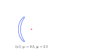
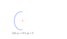
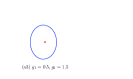
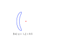
Figure 2: (color online) Several typical graphs obtained from parameter equations in Eq. 58, which characterize the quantum phases for Hermitian and non-Hermitian Ising models. The red dot indicates the origin of the $xy$ plane.

III Chern numbers

In the previous work LC1 PRA , it was found that the Berry phase can be utilized to identify the phase diagram of the non-Hermitian Hamiltonian. We now investigate the connection between quantum phases and other geometric quantity, the Chern number. We start our analysis from the Bloch Hamiltonian $H_{k}$. We will give the derivations in parallel steps for both Hermitian and non-Hermitian Hamiltonians. In both cases, one can rewrite the Hamiltonian in the form

$$H_{k}=\vec{B}_{k}\cdot\vec{s}_{k},$$ (40)

where $\vec{B}_{k}=(0,0,2(\varepsilon_{++}+\varepsilon_{+-}))$ and pseudo spin operators are defined as

$$s_{k}^{-} = \left(s_{k}^{+}\right)^{{\dagger}}=\gamma_{++}^{k}\gamma_{+-}^{k},$$

$$s_{k}^{z} = \frac{1}{2}[\sum_{\sigma=\pm}\left(\gamma_{+\sigma}^{k}\right)^{{\dagger}}\gamma_{+\sigma}^{k}-1],$$ (41)

for real field and

$$s_{k}^{-} = \zeta_{++}^{k}\zeta_{+-}^{k},s_{k}^{+}=\overline{\zeta}_{+-}^{k}\overline{\zeta}_{++}^{k},$$

$$s_{k}^{z} = \frac{1}{2}[\sum_{\sigma=\pm}\overline{\zeta}_{+\sigma}^{k}\zeta_{+\sigma}^{k}-1],$$ (42)

for complex field, satisfying the commutation relations of Lie algebra

$$\left[s_{k}^{z},s_{k^{\prime}}^{\pm}\right]=\pm\delta_{kk^{\prime}}s_{k^{\prime}}^{\pm},\text{ }\left[s_{k}^{+},s_{k^{\prime}}^{-}\right]=2\delta_{kk^{\prime}}s_{k^{\prime}}^{z}.$$ (43)

In order to capture the topological features of the ground states, we map the Hamiltonian $H_{k}$ to $H_{k}(\theta,\varphi)$. It has the form

$$H_{k}(\theta,\varphi)=\vec{B}_{k}(\theta,\varphi)\cdot\vec{s}_{k},$$ (44)

where the field is

$$\vec{B}_{k}(\theta,\varphi)=(\left|\vec{B}_{k}\right|\sin\varphi\cos\theta,\left|\vec{B}_{k}\right|\sin\varphi\sin\theta,\cos\varphi).$$ (45)

Here $\theta$ is taken as

$$\tan\theta_{k}=\frac{\sin k}{\cos k-g_{1}g_{2}},\text{ }$$

$$\text{and }\frac{\sin k}{\cos k-(\eta^{2}+\xi^{2})},$$ (46)

for real and complex fields, respectively. We note that when $\varphi=\pi/2$, $H_{k}(\theta,\varphi)$ has the same spectrum with the original Hamiltonian $H_{k}$.

The eigenstates of $H_{k}(\theta,\varphi)$ in the even particle-number invariant subspace are

$$\left|u_{k}^{\pm}\right\rangle = \frac{1}{\sqrt{\Omega_{k}^{\pm}}}[(\cos\varphi+\varepsilon_{k}^{\pm})(\gamma_{++}^{k}\gamma_{+-}^{k})^{{\dagger}}$$ (48)

$$+\left|\vec{B}_{k}\right|^{2}e^{i\theta}\sin\varphi]\left|\mathrm{Vac}\right\rangle,$$

$$\text{and }\frac{1}{\sqrt{\Omega_{k}^{\pm}}}[(\cos\varphi+\varepsilon_{k}^{\pm})\overline{\zeta}_{+-}^{k}\overline{\zeta}_{++}^{k}$$

$$+\left|\vec{B}_{k}\right|^{2}e^{i\theta}\sin\varphi]\left|\mathrm{Vac}\right\rangle,$$

with $\Omega_{k}^{\pm}=2\left|\varepsilon_{k}^{\pm}\right|\left(\left|\varepsilon_{k}^{\pm}\right|\pm\cos\varphi\right)$, for real and complex fields, respectively. The corresponding eigen energy is

$$\varepsilon_{k}^{\pm}=\pm\sqrt{\cos^{2}\varphi+\left|\vec{B}_{k}\right|^{2}\sin^{2}\varphi}.$$ (49)

We are interested in the ground state, then considering the lower energy level. The Berry connection for $\left|u_{k}^{-}\right\rangle$ is given by

$$A_{k}=i\left\langle u_{k}^{-}\right|\partial_{k}\left|u_{k}^{-}\right\rangle,A_{\varphi}=i\left\langle u_{k}^{-}\right|\partial_{\varphi}\left|u_{k}^{-}\right\rangle,$$ (50)

for real field and

$$A_{k}=i\left\langle\bar{u}_{k}^{-}\right|\partial_{k}\left|u_{k}^{-}\right\rangle,A_{\varphi}=i\left\langle\bar{u}_{k}^{-}\right|\partial_{\varphi}\left|u_{k}^{-}\right\rangle,$$ (51)

for complex field, where $\left\langle\bar{u}_{k}^{-}\right|$ is the biorthonormal conjugation of $\left|u_{k}^{-}\right\rangle$. We would like to point out that the Berry connection here is defined in the framework of biorthonormal inner product for the non-Hermitian system. A straightforward derivation shows that, in both cases, we have

$$A_{k} = -\frac{1}{\Omega_{k}^{-}}\left|\vec{B}_{k}\right|^{2}\sin^{2}\varphi\frac{\partial\theta}{\partial k},$$ (52)

$$A_{\varphi} = 0.$$ (53)

and the Berry curvature is

$$\Omega_{k\varphi} = \partial_{k}A_{\varphi}-\partial_{\varphi}A_{k}$$ (54)

$$= \frac{1}{2(\varepsilon_{k}^{-})^{3}}\left|\vec{B}_{k}\right|^{2}\sin\varphi\frac{\partial\theta}{\partial k}.$$

For the cases with $\left|g_{1}g_{2}\right|\neq 1$ and $\eta^{2}+\xi^{2}\neq 1$, the corresponding Chern number is

$$c = \frac{1}{2\pi}\int_{0}^{\pi}\text{d}\varphi\int_{0}^{2\pi}\text{d}k\Omega_{k\varphi}$$ (55)

$$= -\frac{1}{2\pi}\left[\theta\left(2\pi\right)-\theta\left(0\right)\right],$$

which only depends on the function of $\theta\left(k\right)$ defined in Eq. (46). For the cases with $\left|g_{1}g_{2}\right|=1$ and $\eta^{2}+\xi^{2}=1$, a straightforward derivation shows $c=\frac{1}{2}$. In summary, it is easy to check that the Chern number is

$$c=\left\{\begin{array}[]{cc}1,&\left|g_{1}g_{2}\right|<1\\ \frac{1}{2}&\left|g_{1}g_{2}\right|=1\\ 0,&\left|g_{1}g_{2}\right|>1\end{array}\right.,$$ (56)

for the Hermitian system and

$$c=\left\{\begin{array}[]{cc}1,&\eta^{2}+\xi^{2}<1\\ \frac{1}{2}&\eta^{2}+\xi^{2}=1\\ 0,&\eta^{2}+\xi^{2}>1\end{array}\right.,$$ (57)

for the non-Hermitian system, which accords with the phase diagram. We get the conclusion that the topological quantity, the Chern number can be used to identify the quantum phases. It indicates that the connection between QPT and topological quantity in the Ising model can be extended to more general systems.

This conclusion can be understood from the viewpoint of geometry. We consider the case with $\varphi=\pi/2$, the field reduces to a two-dimensional field. In this plane, the ground state corresponds to a loop depicted by the parameter equations

$$x=\left|\vec{B}_{k}\right|\cos\theta,y=\left|\vec{B}_{k}\right|\sin\theta.$$ (58)

The winding number of a closed curve in the auxiliary $xy$-plane around the origin is defined as

$$\nu=\frac{1}{2\pi}\int\nolimits_{c}\frac{1}{\left|\vec{B}_{k}\right|^{2}}\left(x\mathrm{d}y-y\mathrm{d}x\right),$$ (59)

which has been shown to equal to the Chern number ZG Arxiv . To illustrate this point, we plot the graphs with several typical values of $g_{1}g_{2}$ and $\eta^{2}+\xi^{2}$ in Fig. 2. It clearly shows the connections between the quantum phase diagram and the geometry of the graphs.

IV Summary

We have studied the QPTs in an one-dimensional transverse field Ising model with additional periodically modulated real and complex fields from an alternative view. The equivalent Hamiltonians in the $k$ space allow us to characterize the change of the ground states on passing the phase transition. Based on the exact solution, we have found that the phase boundaries can be identified by the Chern numbers defined in the context of Dirac and biorthonormal inner products, respectively. A notable feature which emerges is that the indicator of the phase transition is not only a local order parameter but also can be the Chern number, which is a key topological quantity. Furthermore, it is available for the non-Hermitian system. An interesting prediction is the extension of such methods to a wider class of quantum spin systems which is consisted of multi-sublattices with the periodic modulation on the coupling strength and field.

References

• (1) X. G. Wen, Int. J. Mod. Phys. B Vol. 04, No. 02, pp. 239-271 (1990).
• (2) G. Zhang and Z. Song, Phys. Rev. Lett. 115, 177204 (2015).
• (3) S. Sachdev, Quantum Phase Transition (Cambridge University Press, Cambridge, 1999).
• (4) C. Li, G. Zhang, X. Z. Zhang, and Z. Song, Phys. Rev. A 90, 012103 (2014).
• (5) C. M. Bender, D. C. Brody, and H. F. Jones, Phys. Rev. Lett. 89, 270401 (2002).
• (6) C. M. Bender and S. Boettcher, Phys. Rev. Lett. 80, 5243 (1998).
• (7) C. M. Bender, S. Boettcher, and P. N. Meisinger, J. Math. Phys. 40, 2201 (1999).
• (8) X. Z. Zhang and Z. Song, Phys. Rev. A 88, 042108 (2013).
• (9) X. Z. Zhang and Z. Song, Phys. Rev. A 87, 012114 (2013).
• (10) G. L. Giorgi, Phys. Rev. B 79, 060405(R) (2009).
• (11) N. Canosa, R. Rossignoli, and J. M. Matera, Phys. Rev. B 81, 054415 (2010).
• (12) G. L. Giorgi, Phys. Rev. B 82, 052404 (2010).
• (13) fidelity.
• (14) P. Jordan and E. Wigner, Z. Physik 47, 631 (1928).
• (15) P. Dorey, C. Dunning, and R. Tateo, J. Phys. A: Math. Gen. 34, L391 (2001); P. Dorey, C. Dunning, and R. Tateo, J. Phys. A: Math. Gen. 34, 5679 (2001).
• (16) A. Mostafazadeh, J. Math. Phys. 43, 3944 (2002).
• (17) A. Mostafazadeh and A. Batal, J. Phys. A: Math. Gen. 37, 11645 (2004).
• (18) A. Mostafazadeh, J. Phys. A: Math. Gen. 36, 7081 (2003).
• (19) H. F. Jones, J. Phys. A: Math. Gen. 38, 1741 (2005).
• (20) A. Mostafazadeh, J. Math. Phys. 43, 2814 (2002).
• (21) G. Zhang, C. Li, and Z. Song, Arxiv:1606.00420 (2016).