Numerical computations on the zeros of the Euler double zeta-function II

Abstract.

We study the behavior of zero-sets of the double zeta-function $\zeta_{2}(s_{1},s_{2})$ (and also of more general multiple zeta-function $\zeta_{r}(s_{1},\ldots,s_{r})$). In our former paper we studied the case $s_{1}=s_{2}$, but in the present paper we consider the more general two variable situation. We carry out numerical computations in order to trace the behavior of zero-sets of $\zeta_{2}(s_{1},s_{2})$. We observe that some zero-sets approach the points $(s_{1},s_{2})$ with $s_{2}=0$, while other zero-sets approach the points $(s_{1},s_{2})$, where $s_{2}$ are solutions of $\zeta(s_{2})=1$. In the former case, when $s_{2}$ tends to $0$, we observe that $\Im s_{1}$ becomes close to the imaginary part of a non-trivial zero of the Riemann zeta-function. In the latter case we give a theoretical proof, in the general $r$-fold setting.

1. Introduction

The present paper is a continuation of the authors’ previous article [5] on the study of the zeros of the Euler double zeta-function

(1.1) $$\zeta_{2}(s_{1},s_{2})=\sum_{n_{1}=1}^{\infty}\sum_{n_{2}=1}^{\infty}\frac{1}{n_{1}^{s_{1}}(n_{1}+n_{2})^{s_{2}}},$$

where $s_{1},s_{2}$ are complex variables. This double series is convergent absolutely in the region defined by $\Re s_{1}+\Re s_{2}>2$ and $\Re s_{2}>1$, and can be continued meromorphically to the whole complex space $\mathbb{C}^{2}$ (see [2]).

This is the case $r=2$ of the more general Euler-Zagier $r$-fold sum

(1.2) $$\zeta_{r}(s_{1},\ldots,s_{r})=\sum_{1\leq n_{1}<\cdots<n_{r}}\frac{1}{n_{1}^{s_{1}}\cdots n_{r}^{s_{r}}},$$

which has been investigated quite extensively from various aspects.

In order to understand the analytic properties of (1.2), it is very important to study the behavior of its zeros and singularities. It is already known that possible singularities of (1.2) are located only on the set $S_{r}$, which is the union of hyperplanes in $\mathbb{C}^{r}$ defined by

$$A_{r}^{(j,n)}:=\{(s_{1},\ldots,s_{r})\in\mathbb{C}^{r}\;|\;s_{r-j+1}+\cdots+s_{r}=j-n\}$$

$$\qquad\qquad\qquad\qquad(n=0,1,2,\ldots,\;2\leq j\leq r),$$

$$A_{r}^{(1)}:=\{(s_{1},\ldots,s_{r})\in\mathbb{C}^{r}\;|\;s_{r}=1\}$$

(see [1], [4]). However, the distribution of the zeros of (1.2) has not been, except for the classical case of $r=1$ (that is the case of the Riemann zeta-function $\zeta(s)$), studied in detail. The aim of the present series of papers is to study the behavior of the zeros of (1.1), the simplest case (except for the case $r=1$), from the viewpoint of numerical computations.

In [5], we considered the situation when $s_{1}=s_{2}(=s)$. Then $\zeta_{2}(s,s)$ is a function of one variable, so we can study the distribution of the zeros of $\zeta_{2}(s,s)$ in a way analogous to the case of $\zeta(s)$. Unlike the case of $\zeta(s)$, the function $\zeta_{2}(s,s)$ does not satisfy the analogue of the Riemann hypothesis. We found a lot of zeros in the strip $0\leq\Re s\leq 1$ off the line $\Re s=1/2$, or even outside that strip (see [5, Observation 1] and [5, Figure 1]). We pointed out that the distribution of those zeros is similar, not to the case of $\zeta(s)$, but rather, to the case of Hurwitz zeta-functions.

In the present paper, we consider the general situation, when $s_{1}$ and $s_{2}$ are moving independently. The zeros of $\zeta_{2}(s_{1},s_{2})$, as a function of two variables, are not isolated points. They form analytic sets in $\mathbb{C}^{2}$, which we call zero-sets. We carry out numerical computations in order to trace the behavior of such zero-sets. Mainly we consider the asymptotic situation of those zero-sets when, for example, $|s_{1}-s_{2}|$ becomes large, or $s_{2}\to 0$, or $|s_{1}|\to\infty$. We observe that some zero-sets approach the points $(s_{1},s_{2})$ with $s_{2}=0$, while other zero-sets approach the points $(s_{1},s_{2})$ where $s_{2}$ are solutions of $\zeta(s_{2})=1$.

It seems that, in general, to give theoretical proofs for the observations described in the present paper is a very difficult task. However, at least, we can construct a proof of the fact that some zero-sets approach the points satisfying $\zeta(s_{2})=1$. In fact, we will prove a more general result for the $r$-fold sum (1.2) in the last section.

Acknowledgment. The authors express their sincere gratitude to the referees for their useful comments and suggestions.

2. The behavior of zero-sets

Our basic strategy is to begin with the zeros of $\zeta_{2}(s,s)$ discovered in [5], and study the behavior of zero-sets of $\zeta_{2}(s_{1},s_{2})$ around those zeros.

Let us begin with [5, Figure 1], which we reproduce here as Figure 1, on which a lot of non-real $s$, for which $\zeta_{2}(s,s)=0$ holds, are dotted. The values of some of which are given in the list written on [5, pp.308-309], whose order is according to the magnitude of the imaginary parts of them. The first four of them are

$$(0.27672860)+i(8.39755368),$$

$$(-0.18995147)+i(12.30422130),$$

$$(0.06443907)+i(15.02312694),$$

$$(-0.53767831)+i(17.58063303).$$

Denote those values by $a_{1},a_{2},a_{3},\ldots$ and so on. (See Remark 1 below for some corrections of the data.)

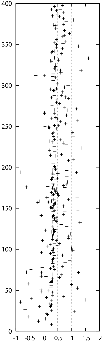
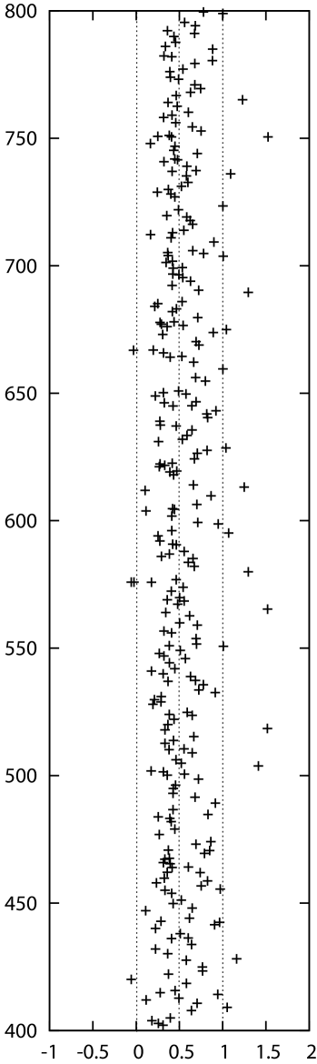
Figure 1. The distribution of zeros of $\zeta_{2}(\sigma+it,\sigma+it)$ for $-1\leq\sigma\leq 2$ and $0\leq t\leq 800$. The horizontal axis represents $\sigma$ and the vertical axis does $t$.

Now consider the two-variable function $\zeta_{2}(s_{1},s_{2})$. Since $\zeta_{2}(s_{1},s_{2})$ cannot have any isolated zero point, the points $(a_{i},a_{i})\in\mathbb{C}^{2}$ are to be intersections of some zero-sets and the hyperplane $s_{1}=s_{2}$. Our first aim is to investigate the behavior of zero-sets near the points $(a_{i},a_{i})$.

Let $\delta$ be a positive number. We search for the zeros of $\zeta_{2}(s_{1},s_{2})$ around the point $(a_{i},a_{i})$ under the condition $|s_{1}-s_{2}|=\delta$. The method of computations is based on the Euler-Maclaurin formula, explained in [5, Section 4]. (It is to be noted that the simple method using the harmonic product formula [5, (2.1), (2.2)] cannot be applied to the present situation where $s_{1}\neq s_{2}$.) Figure 2 describes the loci of the absolute values of zeros satisfying $|s_{1}-s_{2}|=\delta$ around $(a_{i},a_{i})$ ($5\leq i\leq 9$) for various values of $\delta$. We quote the values of those $a_{i}$s from [5]:

$$a_{5}=(0.12844956)+i(20.59707674),$$

$$a_{6}=(0.08804454)+i(21.93232180),$$

$$a_{7}=(1.10778631)+i(23.79708697),$$

$$a_{8}=(0.27268471)+i(24.93425087),$$

$$a_{9}=(-0.67413685)+i(26.88584448).$$

The left one of Figure 2 is the situation when $\delta=0.5$. In this figure we can observe that zero-sets around $(a_{7},a_{7})$ and $(a_{8},a_{8})$ become closer to each other, and it seems that these two zero-sets are connected in the central figure, when $\delta=1$. In the right figure, all the zero-sets around $(a_{5},a_{5})$ to $(a_{8},a_{8})$ seem connected. When $\delta$ becomes larger, more and more zero-sets seem to be connected with each other (see Figure 3).

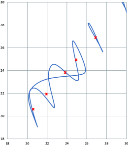
Figure 2. The loci of the absolute values of zeros of $\zeta_{2}(s_{1},s_{2})$ around $(a_{i},a_{i})$ ($5\leq i\leq 9$) with $|s_{1}-s_{2}|=\delta$, where $\delta=0.5$ (left), $1.0$ (center), $2.0$ (right). The horizontal axis represents $|s_{1}|$ and the vertical axis does $|s_{2}|$. The points indicated by the cross marks are $(|a_{5}|,|a_{5}|),(|a_{6}|,|a_{6}|),\ldots,(|a_{9}|,|a_{9}|)$ from the lower-left to the upper-right.

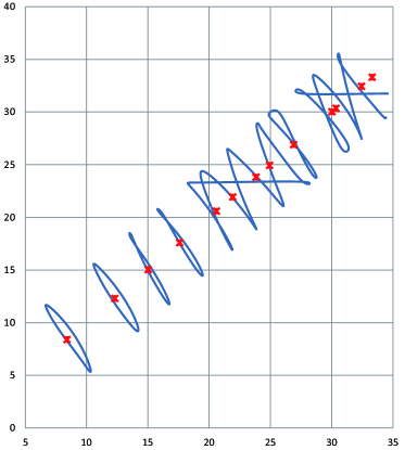
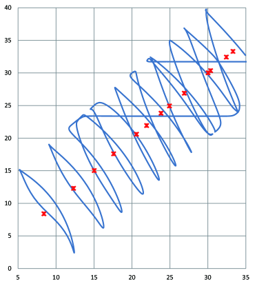
Figure 3. The loci of the absolute values of zeros of $\zeta_{2}(s_{1},s_{2})$ around $(a_{i},a_{i})$ ($1\leq i\leq 13$) with $|s_{1}-s_{2}|=\delta$, where $\delta=5.0$ (left), and $10.0$ (right).

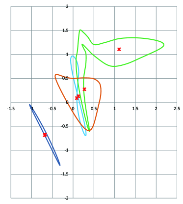
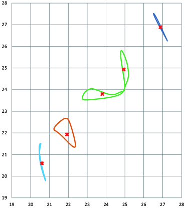
Figure 4. The behavior of real parts and imaginary parts of zeros around $(a_{i},a_{i})$ ($5\leq i\leq 9$) when $\delta=1.0$. On the left figure, the horizontal axis represents $\Re s_{1}$, and the vertical axis does $\Re s_{2}$, while on the right figure they represent $\Im s_{1}$ and $\Im s_{2}$. Since the absolute value is almost determined by the imaginary part (because the real part is relatively small), the right figure is very similar to the central one of Figure 1.

Since Figure 2 only represents the behavior of absolute values, in order to make sure that the above zero-sets are indeed connected, it is necessary to investigate the values of real parts and imaginary parts of those. Figure 4 gives such data. This figure shows that the loci of zeros around $(a_{7},a_{7})$ and $(a_{8},a_{8})$ are indeed connected.

From Figure 3 it seems that all zero-sets appearing in this figure are connected. (The zero-sets including the points $(a_{1},a_{1})$ and $(a_{2},a_{2})$ are not connected to the other zero-sets on the figure, but further computations show that these zero-sets look connected also, when $\delta$ becomes larger.)

From this observation, perhaps we may expect that all points

$$(a_{1},a_{1}),(a_{2},a_{2}),(a_{3},a_{3}),\ldots$$

are lying on the same (unique?) zero-set. However, later in Section 4 we will see that the behavior of some zero-sets is rather different. Probably it is too early to raise any conjecture on the global behavior of zero-sets.

Remark 1.

In [5, p.308], it is noted that the left-most zero in [5, Figure 1] is

$$(-0.830372)+i(35.603804).$$

However, there is at least one zero of $\zeta_{2}(s,s)$ which is located more left. When the authors wrote [5], they overlooked the following two zeros:

$$(-0.874058504)+i(44.93750365),$$

$$(-0.710036436)+i(53.91464901).$$

3. Approaching the axis $s_{2}=0$

From Figure 3 we can observe that, when $\delta$ becomes larger, the shape of the curves consisting of zeros also becomes larger, and the bottoms of the curves look approaching to the horizontal axis (that is, the axis $s_{2}=0$). Figure 5 describes the curves of the absolute values of zeros when $\delta=14.0$. In this case one curve indeed touches the horizontal axis.

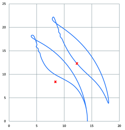
Figure 5. The loci of the absolute values of zeros of $\zeta_{2}(s_{1},s_{2})$ around $(a_{1},a_{1})$ and $(a_{2},a_{2})$ with $|s_{1}-s_{2}|=\delta$, where $\delta=14.0$. The horizontal axis represents $|s_{1}|$ and the vertical axis does $|s_{2}|$.

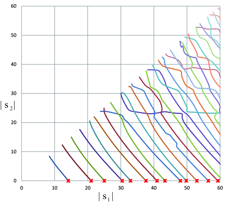
Figure 6. The absolute values of zeros satisfying $s_{2}=\eta s_{1}$, where $1\geq\eta\geq 0$. The horizontal axis represents $|s_{1}|$ (up to $60$) and the vertical axis does $|s_{2}|$. The cross marks represent the absolute values of zeros of $\zeta(s)$.

How about the behavior of other curves? To investigate this point, now we use an alternative way of calculating zeros. Consider the equation $s_{2}=\eta s_{1}$. In [5], we studied the zeros under the condition $\eta=1$. Starting with the data of those zeros, we search for the zeros for various values of $\eta$, $1\geq\eta\geq 0$. When $\eta\to 0$, we find that almost all curves consisting of zeros tend to the horizontal axis (see Figure 6).

Table 1. The left is the list of the values of $s_{1}$ of the points where the curves touch the horizontal axis. The right is the list of non-trivial zeros of $\zeta(s)$.

$(1.247595281)+i(14.14857043)$	$(0.5)+i(14.13472514)$
$(1.279113136)+i(21.01244258)$	$(0.5)+i(21.02203964)$
$(1.292752716)+i(25.03054326)$	$(0.5)+i(25.01085758)$
$(1.304538379)+i(30.39099998)$	$(0.5)+i(30.42487613)$
$(1.310484619)+i(32.97276761)$	$(0.5)+i(32.93506159)$
$(1.319356152)+i(37.57182573)$	$(0.5)+i(37.58617816)$
$(1.320370441)+i(40.90318345)$	$(0.5)+i(40.91871901)$
$(1.328328378)+i(43.36573059)$	$(0.5)+i(43.32707328)$
$(1.333209526)+i(47.94829355)$	$(0.5)+i(48.00515088)$
$(1.330151768)+i(49.81347595)$	$(0.5)+i(49.77383248)$
$(1.338852528)+i(52.98250152)$	$(0.5)+i(52.97032148)$
$(1.341784096)+i(56.42981942)$	$(0.5)+i(56.44624769)$
$(1.336083544)+i(59.30477438)$	$(0.5)+i(59.34704400)$
$(1.347599692)+i(60.90235918)$	$(0.5)+i(60.83177852)$
$(1.350310992)+i(65.06828349)$	$(0.5)+i(65.11254405)$
$(1.343496503)+i(67.09040611)$	$(0.5)+i(67.07981053)$
$(1.348806781)+i(69.55741541)$	$(0.5)+i(69.54640171)$
$(1.354734356)+i(72.08670993)$	$(0.5)+i(72.06715767)$
$(1.356705834)+i(75.63889778)$	$(0.5)+i(75.70469069)$
$(1.344904017)+i(77.17673184)$	$(0.5)+i(77.14484007)$
$(1.360065509)+i(79.37508073)$	$(0.5)+i(79.33737502)$
$(1.360772059)+i(82.86977267)$	$(0.5)+i(82.91038085)$
$(1.355304386)+i(84.75005063)$	$(0.5)+i(84.73549298)$
$(1.353373038)+i(87.38999143)$	$(0.5)+i(87.42527461)$
$(1.365347698)+i(88.87469754)$	$(0.5)+i(88.80911121)$
$(1.367563235)+i(92.45429247)$	$(0.5)+i(92.49189927)$
$(1.352878941)+i(94.60615786)$	$(0.5)+i(94.65134404)$
$(1.364213735)+i(95.93955674)$	$(0.5)+i(95.87063423)$
$(1.367791276)+i(98.82956582)$	$(0.5)+i(98.83119422)$

From Figure 6 we observe that the values $|s_{1}|$ of the points $(s_{1},s_{2})$ at which the loci touch the horizontal axis are almost the same as the absolute values of zeros of $\zeta(s)$. Let us list up those values. The left of Table 1 is the list of the values of $s_{1}$ of the points where the curves touch the horizontal axis. Comparing this table with the list of non-trivial zeros of $\zeta(s)$ (the right of Table 1), we find:

Observation 1.

The imaginary part of each $s_{1}$ in the left list of Table 1 is very close to an imaginary part of a value appearing in the right list of Table 1, that is, a non-trivial zero of $\zeta(s)$.

The following argument is not rigorous, but at least heuristically, explains this observation.

Recall the formula [5, (2.3)] (originally in [1]):

(3.1) $$\zeta_{2}(s_{1},s_{2})=\frac{\zeta(s_{1}+s_{2}-1)}{s_{2}-1}-\frac{\zeta(s_{1}+s_{2})}{2}$$

$$\qquad+\sum_{q=1}^{l}(s_{2})_{q}\frac{B_{q+1}}{(q+1)!}\zeta(s_{1}+s_{2}+q)-\sum_{n_{1}=1}^{\infty}\frac{\phi_{l}(n_{1},s_{2})}{n_{1}^{s_{1}}},$$

where $(s_{2})_{q}=s_{2}(s_{2}+1)\cdots(s_{2}+q-1)$, $B_{q+1}$ is the $(q+1)$-th Bernoulli number, and

$$\phi_{l}(n_{1},s_{2})$$

$$=\sum_{k=1}^{n}\frac{1}{k^{s}}-\left\{\frac{n^{1-s}-1}{1-s}+\frac{1}{2n^{s}}-\sum_{q=1}^{l}\frac{(s)_{q}B_{q+1}}{(q+1)!n^{s+q}}+\zeta(s)-\frac{1}{s-1}\right\}$$

(see [5, (2.4)]). Put $s_{2}=0$ in (3.1). Since $\phi_{l}(n_{1},0)=0$ (which can be seen by [5, (2.5)]), we find that the two sums on the right-hand side of (3.1) are both zero, so

(3.2) $$\zeta_{2}(s_{1},0)=-\zeta(s_{1}-1)-\frac{\zeta(s_{1})}{2}.$$

Now, let $s_{1}^{*}$ be one of the values in the left list of Table 1. Then $\zeta_{2}(s_{1}^{*},0)=0$, so (3.2) implies

(3.3) $$\zeta(s_{1}^{*})=-2\zeta(s_{1}^{*}-1).$$

Let

$$C(t)=\{\zeta(\sigma+it)\;|\;\sigma\in\mathbb{R}\}.$$

If $t$ is very close to the imaginary part of a non-trivial zero of $\zeta(s)$, the graph of the curve $C(t)$ passes very close to the origin when $\sigma=1/2$ (see Figure 7). As can be seen from Figure 7, when $\sigma$ moves, the slope of the graph of $C(t)$ does not so rapidly change. This can be naturally expected, because the approximate functional equation of $\zeta(s)$ (see [6, Theorem 4.15]) implies that the behavior of $\zeta(s)$ is dominated by the terms of the form $n^{-s}=n^{-\sigma}e^{-it\log n}$, and if $t$ is fixed, then the “argument” part of these terms does not change.

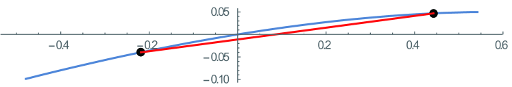
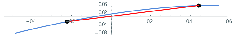
Figure 7. The first one is the locus of $\zeta(\sigma+it_{0})$, where $t_{0}=14.13472514$ (= the first of the right list of Table 1). Therefore this locus crosses the origin. The two black-dots represent the points $s(t_{0})=(0.442629)+i(0.0469269)$ and $s(t_{0}-1)=(-0.218684)-i(0.0397677)$, with $\sigma(t_{0})=1.2475$. This satisfies (3.4). The second one is the locus of $\zeta(\sigma+it_{0}^{*})$, where $t_{0}^{*}=14.14857043$ (= the first of the left list of Table 1), for which $L(t_{0}^{*})$ crosses the origin.

Therefore we can find a number $\sigma(t)\in\mathbb{R}$ such that

(3.4) $$|\zeta(s(t))|=2|\zeta(s(t)-1)|,$$

where $s(t)=\sigma(t)+it$. We denote by $L(t)$ the segment joining $\zeta(s(t))$ and $\zeta(s(t)-1)$.

Now choose $t=t_{0}$, for which $(1/2)+it_{0}$ is in the right list of Table 1. Then, as in the first one of Figure 7 (where the case $t_{0}=14.13472514$ is described), $\arg\zeta(s(t_{0})-1)$ is almost equal to $\arg\zeta(s(t_{0}))\pm\pi$, so $L(t_{0})$ passes very close to the origin. (If $C(t_{0})$ would be a straight line, then $L(t_{0})$ could indeed cross the origin; but this is not the case.) Move the value of $t$ a little from $t_{0}$. Then the curve $C(t)$ also moves a little. Then, as in the second one of Figure 7, we may find a value of $t=t_{0}^{*}$, close to $t_{0}$, for which $L(t_{0}^{*})$ indeed crosses the origin. This implies $\zeta(s(t_{0}^{*}))=-2\zeta(s(t_{0}^{*})-1)$, that is, in view of (3.3), this $s(t_{0}^{*})=\sigma(t_{0}^{*})+it_{0}^{*}$ should be in the left list of Table 1.

It is an interesting problem to make the above argument more rigorous, and to get some formula which expresses the phenomenon of Observation 1.

Remark 2.

It is also observed that the real parts of the points on the list of Table 1 are close to each other, around the value $1.3$. So far we have not found any theoretical reasoning of this phenomenon.

4. Approaching the zeros of $\zeta(s)=1$

In Figure 6, we can observe that almost all curves approach the horizontal axis. However, when we extend the range of computations, we find that there are curves which do not seem to approach the horizontal axis (Figure 8). Along these curves, it seems that $|s_{1}|$ becomes larger and larger.

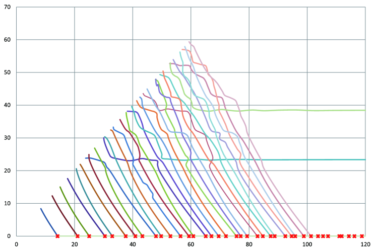
Figure 8. This figure represents the same computations as in Figure 6, but the range of $|s_{1}|$ is up to $120$. The cross marks represent the absolute values of zeros of $\zeta(s)$. There appear two curves which do not approach the horizontal axis.

Moreover, extending the range of computations, we can find more zero-sets, along them $|s_{1}|$ seems to tend to infinity (see Figure 9).

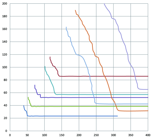
Figure 9. The same computations as in Figure 6, but the range of $|s_{1}|$ is up to $400$. Only the curves which do not approach the horizontal axis are drawn.

The numerical data suggests that $\Re s_{1}$ tends to infinity along these curves (the left of Figure 10), while $\Re s_{2}$ remains finite (the right of Figure 10).

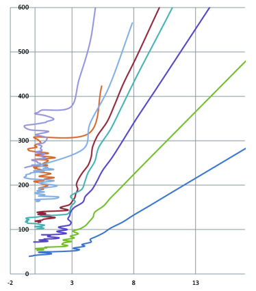
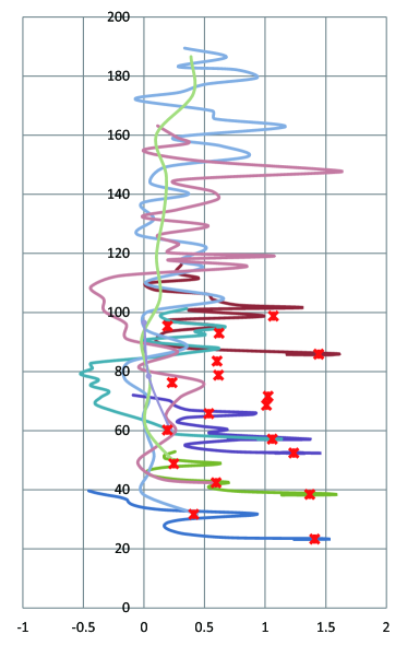
Figure 10. The behavior of $s_{1}$ (left) and $s_{2}$ (right) of curves described in Figure 9. The cross marks on the right figure are solutions of $\zeta(s_{2})=1$. There may be more solutions, but we only mark the solutions we found numerically.

What happens? We can prove the following facts.

Proposition 1.

(i) Let $(s_{1}^{(m)},s_{2}^{(m)})$ $(m=1,2,\ldots)$ be a sequence of points on a zero-divisor of $\zeta_{2}(s_{1},s_{2})$. If $\sigma_{1}^{(m)}=\Re s_{1}^{(m)}$ tends to infinity and $|s_{2}^{(m)}|$ remains bounded (and not close to $1$) as $m\to\infty$, then $s_{2}^{(m)}$ tends to a solution of $\zeta(s_{2})=1$.

(ii) Conversely, for any solution $\rho_{2}$ of $\zeta(\rho_{2})=1$ and any $\varepsilon>0$, we can find a zero of $\zeta_{2}(s_{1},s_{2})$ such that $|s_{2}-\rho_{2}|<\varepsilon$.

This result is due to Professor Seidai Yasuda (Osaka University). The authors express their sincere gratitude to him for the permission of including his result in the present paper.

In the next section we will state general theorems on the asymptotic behavior of zero-sets of $r$-fold sum (1.2). The above proposition is just a special case of those theorems.

Remark 3.

The assertion (i) of the above proposition is, if $\Re s_{2}>1$, obvious. Because in this case we can use (1.1). Letting $\Re s_{1}\to\infty$ on (1.1), we see that the right-hand side tends to $\sum_{n_{2}=1}^{\infty}(1+n_{2})^{-s_{2}}=\zeta(s_{2})-1$.

5. The asymptotic behavior of zero-sets of the $r$-fold sum

We study the behavior of $\zeta_{r}(s_{1},\ldots,s_{r})$ when $\sigma_{k}=\Re s_{k}$ for some $k$ tends to $+\infty$ while the other variables remain bounded. We write $\mathbb{C}^{r}=\mathbb{C}_{(k)}^{r-1}\times\mathbb{C}_{(k)}$, where $\mathbb{C}_{(k)}^{r-1}$ consists of all $(s_{1},\ldots,s_{k-1},s_{k+1},\ldots,s_{r})$ and $\mathbb{C}_{(k)}$ denotes the $s_{k}$-plane. Let $S_{k,r}$ be the union of all hyperplanes $A_{j,n}$ and $A_{1}$ (defined in Section 1) whose defining equation does not include $s_{k}$. That is,

$$S_{k,r}=\Bigl{(}\bigcup_{2\leq j\leq r-k}\bigcup_{n=0}^{\infty}A_{r}^{(j,n)}\Bigr{)}\bigcup A_{r}^{(1)}\qquad(1\leq k\leq r-2),$$

$S_{r-1,r}=A_{r}^{(1)}$, and $S_{r,r}=\emptyset$.

First, when $k\geq 2$, the conclusion is simple.

Theorem 1.

Let $r\geq 2$, $2\leq k\leq r$, and $E_{k,r-1}$ a closed subset of $\mathbb{C}_{(k)}^{r-1}$ such that

$$\{(\sigma_{1},\ldots,\sigma_{k-1},\sigma_{k+1},\ldots,\sigma_{r})\;|\;(s_{1},\ldots,s_{k-1},s_{k+1},\ldots,s_{r})\in E_{k,r-1}\}$$

is bounded, and

(5.1) $$(E_{k,r-1}\times\mathbb{C}_{(k)})\cap S_{k,r}=\emptyset.$$

When $\sigma_{k}=\Re s_{k}$ tends to $+\infty$ while the other variables remain in $E_{k,r-1}$, the value $\zeta_{r}(s_{1},\ldots,s_{r})$ tends to $0$, uniformly in $E_{k,r-1}$.

More interesting is the situation when $k=1$. Let $r\geq 1$, and define

(5.2) $$F_{r-1}(s_{2},\ldots,s_{r})=\sum_{j=1}^{r-1}(-1)^{r-j+1}\zeta_{j}(s_{r-j+1},\ldots,s_{r})-(-1)^{r}.$$

(When $r=1$, we understand simply that $F_{0}=1$.) Denote by $\mathcal{H}_{r-1}$ the hypersurface in the space $\mathbb{C}_{(1)}^{r-1}$ defined by the equation

(5.3) $$F_{r-1}(s_{2},\ldots,s_{r})=0.$$

Theorem 2.

Let $D_{r-1}$ a bounded closed subset of $\mathbb{C}_{(1)}^{r-1}$ such that

(5.4) $$(D_{r-1}\times\mathbb{C}_{(1)})\cap S_{1,r}=\emptyset.$$

Let $(s_{1}^{(m)},\ldots,s_{r}^{(m)})$ $(m=1,2,3,\ldots)$ be a sequence of points in $\mathbb{C}^{r}$. Assume that, as $m\to\infty$, $\sigma_{1}^{(m)}=\Re s_{1}^{(m)}$ tends to $+\infty$ while $(s_{2}^{(m)},\ldots,s_{r}^{(m)})$ remains in $D_{r-1}$. Then for any $\varepsilon>0$, we can choose a sufficiently large $M$, uniformly in $D_{r-1}$, for which

(5.5) $$|\zeta_{r}(s_{1}^{(m)},\ldots,s_{r}^{(m)})-F_{r-1}(s_{2}^{(m)},\ldots,s_{r}^{(m)})|<\varepsilon$$

holds for any $m\geq M$.

Theorem 3.

Assume $r\geq 2$.

(i) Let $(s_{1}^{(m)},\ldots,s_{r}^{(m)})$ $(m=1,2,3,\ldots)$ be a sequence of points on a zero-set of $\zeta_{r}(s_{1},\ldots,s_{r})$. Assume that $\sigma_{1}^{(m)}=\Re s_{1}^{(m)}$ tends to $+\infty$ while $(s_{2}^{(m)},\ldots,s_{r}^{(m)})$ remains in $D_{r-1}$ (as in the statement of Theorem 2). Then, uniformly on $D_{r-1}$, the sequence $(s_{2}^{(m)},\ldots,s_{r}^{(m)})$ is approaching the hypersurface $\mathcal{H}_{r-1}$. Therefore, we can find a subsequence $(s_{2}^{(k_{m})},\ldots,s_{r}^{(k_{m})})$ $(m=1,2,3,\ldots)$ which converges to a point $(\rho_{2},\ldots,\rho_{r})$ on $\mathcal{H}_{r-1}$.

(ii) Conversely, for any solution $(\rho_{2},\ldots,\rho_{r})$ of (5.3), we can find a sequence $(s_{1}^{(m)},\ldots,s_{r}^{(m)})$ $(m=1,2,3,\ldots)$ on a zero-set of $\zeta_{r}(s_{1},\ldots,s_{r})$ which converges to $(\rho_{2},\ldots,\rho_{r})$.

The case $r=2$ of Theorem 3 is exactly Proposition 1 given in the previous section.

6. Proofs of theorems

We begin with the proof of Theorem 1.

Proof of Theorem 1.

We divide the proof into several steps.

Step 1.  The multiple series

(6.1) $$\zeta_{r}(s_{1},\ldots,s_{r})=\sum_{n_{1}=1}^{\infty}\cdots\sum_{n_{r}=1}^{\infty}n_{1}^{-s_{1}}(n_{1}+n_{2})^{-s_{2}}\cdots(n_{1}+\cdots+n_{r})^{-s_{r}}$$

($r\geq 2$) is absolutely convergent when $\sigma_{r}$ is sufficiently large. Since $n_{1}+\cdots+n_{r}\geq r\geq 2$, all the terms on the right-hand side tend to 0 when $\sigma_{r}\to\infty$, uniformly in $(s_{1},\ldots,s_{r-1})\in E_{r,r-1}$. Hence the assertion in the case $k=r$ follows.

Step 2.  However in the case $\sigma_{k}\to\infty$ $(2\leq k\leq r-1)$, the above argument is not enough, because if $\sigma_{r}$ is not large, then the expression (6.1) is not valid. Therefore we first carry out the meromorphic continuation.

We prove the continuation by induction. Assume that $\zeta_{r-1}(s_{1},\ldots,s_{r-1})$ can be continued meromorphically to the whole space $\mathbb{C}^{r-1}$.

Here, we apply the method of using the Mellin-Barnes integral formula

(6.2) $$(1+\lambda)^{-s}=\frac{1}{2\pi i}\int_{(c)}\frac{\Gamma(s+z)\Gamma(-z)}{\Gamma(s)}\lambda^{z}dz,$$

where $s,\lambda\in\mathbb{C}$, $\Re s>0$, $\lambda\neq 0$, $|\arg\lambda|<\pi$, $-\Re s<c<0$, and the path of integration is the vertical line $\Re z=c$. The following argument was done (in a more general form) in [3] [4]. Assume, at first, that $\Re s_{k}>1$ for all $1\leq k\leq r$. Then (6.1) is absolutely convergent, and an application of (6.2) yields

(6.3) $$\zeta_{r}(s_{1},\ldots,s_{r})=\frac{1}{2\pi i}\int_{(c)}\frac{\Gamma(s_{r}+z)\Gamma(-z)}{\Gamma(s_{r})}$$

$$\;\times\zeta_{r-1}(s_{1},\ldots,s_{r-2},s_{r-1}+s_{r}+z)\zeta(-z)dz$$

(see [3, (12.3)]), where $-\Re s_{r}<c<-1$. Then we shift the path of integration to the line $\Re z=M-\varepsilon$, where $M$ is a large positive integer and $\varepsilon$ is a small positive number. Counting the relevant residues, we obtain

(6.4) $$\zeta_{r}(s_{1},\ldots,s_{r})=\frac{1}{s_{r}-1}\zeta_{r-1}(s_{1},\ldots,s_{r-2},s_{r-1}+s_{r}-1)$$

$$+\sum_{l=0}^{M-1}\binom{-s_{n}}{l}\zeta_{r-1}(s_{1},\ldots,s_{r-2},s_{r-1}+s_{r}+l)\zeta(-l)$$

$$+\frac{1}{2\pi i}\int_{(M-\varepsilon)}\frac{\Gamma(s_{r}+z)\Gamma(-z)}{\Gamma(s_{r})}$$

$$\quad\times\zeta_{r-1}(s_{1},\ldots,s_{r-2},s_{r-1}+s_{r}+z)\zeta(-z)dz$$

(see [3, (12.7)]). Since the last integral is convergent in the wider region

(6.5) $$\{(s_{1},\ldots,s_{r})\;|\;\Re(s_{r-j+1}+\cdots+s_{r})>j-1-M+\varepsilon\;(1\leq j\leq r)\}$$

(see [3, (12.9)]), we find that $\zeta_{r}(s_{1},\ldots,s_{r})$ can be continued to this region. Since $M$ is arbitrary, (6.4) implies the meromorphic continuation of $\zeta_{r}(s_{1},\ldots,s_{r})$ to the whole space $\mathbb{C}^{r}$.

Step 3.  Let $2\leq k\leq r-1$, and we prove the theorem in this case by induction on $r$. Note that the theorem in the case $r=2$ has been already proved in Step 1. Assume the theorem is true for $r-1$, and consider the situation:

$(*)$ $\sigma_{k}=\Re s_{k}$ tends to $+\infty$, while the other variables remain in the region $E_{k,r-1}$.

Assume that $(s_{1},\ldots,s_{r})$ is under the situation $(*)$. Then it is clearly included in the above region (6.5) for sufficiently large $M$, so we can use the expression (6.4). Therefore our aim is to show that the right-hand side of (6.4) tends to 0 when $\sigma_{k}\to\infty$.

First note that the factor $(s_{r}-1)^{-1}$ remains bounded. This is because (5.1) especially implies $(E_{k,r-1}\times\mathbb{C}_{(k)})\cap A_{r}^{(1)}=\emptyset$.

When $k=r-1$, we see that the real part of the last variable tends to $+\infty$ in all the $\zeta_{r-1}(\cdot)$ factors on the right-hand side of (6.4). Therefore we can conclude that the right-hand side of (6.4) tends to 0 as $\sigma_{r-1}\to\infty$, as in Step 1.

Step 4.  Assume $2\leq k\leq r-2$. Then we can define

$$E_{k,r-1}^{w}=\left\{(s_{1},\ldots,s_{k-1},s_{k+1},\ldots,s_{r-2},s_{r-1}+s_{r}+w)\;|\right.$$

$$\left.\quad(s_{1},\ldots,s_{k-1},s_{k+1},\ldots,s_{r})\in E_{k,r-1}\right\}\subset\mathbb{C}^{r-2},$$

where $w=-1,0,1,2,\ldots,M-1$. These $E_{k,r-1}^{w}$ are all closed subsets whose real parts are bounded.

We claim

(6.6) $$(E_{k,r-1}^{w}\times\mathbb{C}_{(k)})\cap S_{k,r-1}=\emptyset\qquad(w=-1,0,1,2,\ldots,M-1).$$

In fact, if

$$(s_{1},\ldots,s_{r-2},s_{r-1}+s_{r}+w)$$

$$=((s_{1},\ldots,s_{k-1},s_{k+1},\ldots,s_{r-2},s_{r-1}+s_{r}+w),s_{k})$$

$$\in(E_{k,r-1}^{w}\times\mathbb{C}_{(k)})\cap S_{k,r-1},$$

then $(s_{1},\ldots,s_{r-2},s_{r-1}+s_{r}+w)\in A_{r-1}^{(j,n)}$ for some $j\in\{2,\ldots,r-1-k\}$ and some $n\geq 0$, or $(s_{1},\ldots,s_{r-2},s_{r-1}+s_{r}+w)\in A_{r-1}^{(1)}$. The former case implies

$$s_{r-1-j+1}+\cdots+s_{r-2}+(s_{r-1}+s_{r}+w)=j-n,$$

so $s_{r-j}+\cdots+s_{r}=j-n-w$, and the latter case implies $s_{r-1}+s_{r}=1-w$. Therefore we conclude that $(s_{1},\ldots,s_{r})\in S_{k,r}$, which contradicts with the assumption (5.1). The claim (6.6) follows.

Therefore we can apply the induction assumption to the factors

$$\zeta_{r-1}(s_{1},\ldots,s_{r-2},s_{r-1}+s_{r}+w)\qquad(w=-1,0,1,2,\ldots,M-1)$$

on the right-hand side of (6.4) to find that these factors tends to 0 under the assumption $(*)$.

Lastly we consider the integral term. We may choose $M$ in (6.4) sufficiently large so that the factor $\zeta_{r-1}(s_{1},\ldots,s_{r-2},s_{r-1}+s_{r}+z)$ in the integrand is convergent absolutely. Then

$$\zeta_{r-1}(s_{1},\ldots,s_{r-2},s_{r-1}+s_{r}+z)$$

$$=\sum_{n_{1}=1}^{\infty}\cdots\sum_{n_{r-1}=1}^{\infty}n_{1}^{-s_{1}}\cdots(n_{1}+\cdots+n_{r-2})^{-s_{r-2}}(n_{1}+\cdots+n_{r-1})^{-s_{r-1}-s_{r}-z},$$

and since $n_{1}+\cdots+n_{k}\geq k\geq 2$, this vanishes when $\sigma_{k}\to\infty$. This completes the proof of the theorem.

∎

Next we proceed to the proof of Theorem 2. The assertion (i) of Theorem 3 is clearly a special case of Theorem 2, that is, the case $\zeta_{r}(s_{1}^{(m)},\ldots,s_{r}^{(m)})=0$ in (5.5).

Proof of Theorem 2.

When $r=1$, the assertion of the theorem is $\zeta(s_{1}^{(m)})\to 1$ as $\sigma_{1}^{(m)}\to+\infty$, which is obvious. We assume that the theorem is true for $r-1$, and prove the theorem by induction. We use the following harmonic product formula.

(6.7) $$\zeta(s_{1})\zeta_{r-1}(s_{2},\ldots,s_{r})$$

$$\;=\sum_{n_{1}=1}^{\infty}n_{1}^{-s_{1}}\sum_{n_{2}<\cdots<n_{r}}n_{2}^{-s_{2}}\cdots n_{r}^{-s_{r}}$$

$$\;=\sum_{n_{1}<n_{2}<\cdots<n_{r}}+\sum_{n_{1}=n_{2}<n_{3}<\cdots<n_{r}}+\sum_{n_{2}<n_{1}<n_{3}<\cdots<n_{r}}$$

$$\quad+\sum_{n_{2}<n_{1}=n_{3}<\cdots<n_{r}}+\cdots+\sum_{n_{2}<\cdots<n_{r-1}<n_{1}<n_{r}}$$

$$\quad+\sum_{n_{2}<\cdots<n_{r-1}<n_{1}=n_{r}}+\sum_{n_{2}<\cdots<n_{r-1}<n_{r}<n_{1}}$$

$$\;=\zeta_{r}(s_{1},s_{2},\ldots,s_{r})+\zeta_{r-1}(s_{1}+s_{2},s_{3},\ldots,s_{r})+\zeta_{r}(s_{2},s_{1},s_{3},\ldots,s_{r})$$

$$\quad+\zeta_{r-1}(s_{2},s_{1}+s_{3},\ldots,s_{r})+\cdots+\zeta_{r}(s_{2},\ldots,s_{r-1},s_{1},s_{r})$$

$$\quad+\zeta_{r-1}(s_{2},\ldots,s_{r-1},s_{1}+s_{r})+\zeta_{r}(s_{2},\ldots,s_{r-1},s_{r},s_{1}),$$

which is first valid in the region $\Re s_{k}>1$ ($1\leq k\leq r$), but then is valid in the whole space by meromorphic continuation.

Let $s_{k}=s_{k}^{(m)}$ ($1\leq k\leq r$) in (6.7), and consider the situation when $\sigma_{1}^{(m)}\to+\infty$ and $(s_{2}^{(m)},\ldots,s_{r}^{(m)})$ remains in $D_{r-1}$.

The singularities appearing in the formula (6.7) consist of two types: included in $S_{1,r}$, or some hyperplane whose defining equation includes $s_{1}$. Therefore by (5.4) we find that those singularities are irrelevant during our process $\sigma_{1}^{(m)}\to+\infty$.

Therefore $\zeta_{r-1}(s_{2}^{(m)},\ldots,s_{r}^{(m)})$ remains bounded. Noting $\zeta(s_{1}^{(m)})\to 1$ we see that there exists a large $M_{1}=M_{1}(\varepsilon)$ for which

(6.8) $$|\zeta(s_{1}^{(m)})\zeta_{r-1}(s_{2}^{(m)},\ldots,s_{r}^{(m)})-\zeta_{r-1}(s_{2}^{(m)},\ldots,s_{r}^{(m)})|<\varepsilon/3$$

holds for any $m\geq M_{1}$.

On the right-hand side of (6.7), denote by $G(s_{1},\ldots,s_{r})$ the sum of all the terms, except for the first two terms. Then $G(s_{1}^{(m)},\ldots,s_{r}^{(m)})$ tends to 0, in view of Theorem 1. That is, there exists $M_{2}=M_{2}(\varepsilon)$ for which

(6.9) $$|G(s_{1}^{(m)},\ldots,s_{r}^{(m)})|<\varepsilon/3$$

holds for any $m\geq M_{2}$.

We use the induction assumption to treat the second term on the right-hand side. We can find $M_{3}=M_{3}(\varepsilon)$ for which

(6.10) $$|\zeta_{r-1}(s_{1}^{(m)}+s_{2}^{(m)},s_{3}^{(m)},\ldots,s_{r}^{(m)})-F_{r-2}(s_{3}^{(m)},\ldots,s_{r}^{(m)})|<\varepsilon/3$$

for any $m\geq M_{3}$.

Substituting (6.8), (6.9) and (6.10) into (6.7) we find that

$$|\zeta_{r}(s_{1}^{(m)},\ldots,s_{r}^{(m)})-(\zeta_{r-1}(s_{2}^{(m)},\ldots,s_{r}^{(m)})-F_{r-2}(s_{3}^{(m)},\ldots,s_{r}^{(m)}))|$$

$$\qquad<\varepsilon/3+\varepsilon/3+\varepsilon/3,$$

that is,

$$|\zeta_{r}(s_{1}^{(m)},\ldots,s_{r}^{(m)})-F_{r-1}(s_{2}^{(m)},\ldots,s_{r}^{(m)})|<\varepsilon.$$

The uniformity of the convergence follows from the assertion on the uniformity in Theorem 1. This completes the proof of Theorem 2, and hence the part (i) of Theorem 3. ∎

Remark 4.

(A generalization of Remark 3) If $\Re s_{r}>1$, then (6.1) is valid. In this case, when $\sigma_{1}\to+\infty$ and $(s_{2}^{(m)},\ldots,s_{r}^{(m)})$ tends to $(\rho_{2},\ldots,\rho_{r})$, from (6.1) it is immediate that $\zeta_{r}(s_{1}^{(m)},\ldots,s_{r}^{(m)})$ tends to

(6.11) $$\sum_{n_{2}=1}^{\infty}\cdots\sum_{n_{r}=1}^{\infty}(1+n_{2})^{-\rho_{2}}\cdots(1+n_{2}+\cdots+n_{r})^{-\rho_{r}}.$$

Therefore in the region $\Re s_{r}>1$, the two expressions $F_{r-1}(\rho_{2},\ldots,\rho_{r})$ and (6.11) should be equal to each other. In fact, putting $1+n_{2}=m_{2}$ in (6.11), we see that (6.11) is equal to

$$\sum_{m_{2}=2}^{\infty}\sum_{n_{3}=1}^{\infty}\cdots\sum_{n_{r}=1}^{\infty}m_{2}^{-\rho_{2}}(m_{2}+n_{3})^{-\rho_{3}}\cdots(m_{2}+n_{3}+\cdots+n_{r})^{-\rho_{r}}$$

$$=\zeta_{r-1}(\rho_{2},\rho_{3},\ldots,\rho_{r})-\sum_{n_{3}=1}^{\infty}\cdots\sum_{n_{r}=1}^{\infty}(1+n_{3})^{-\rho_{3}}\cdots(1+n_{3}+\cdots+n_{r})^{-\rho_{r}}.$$

Next we put $1+n_{3}=m_{3}$ and argue similarly to obtain that the second sum on the right-hand side is

$$=\zeta_{r-2}(\rho_{3},\ldots,\rho_{r})-\sum_{n_{4}=1}^{\infty}\cdots\sum_{n_{r}=1}^{\infty}(1+n_{4})^{-\rho_{4}}\cdots(1+n_{4}+\cdots+n_{r})^{-\rho_{r}}.$$

Repeating this argument, we arrive at the expression $F_{r-1}(\rho_{2},\ldots,\rho_{r})$.

Lastly we prove the part (ii) of Theorem 3. Let $(\rho_{2},\ldots,\rho_{r})$ be any solution of (5.3). We fix $\rho_{2},\ldots,\rho_{r-1}$, and regard $F_{r-1}(\rho_{2},\ldots,\rho_{r-1},s_{r})$ as a function of one complex variable $s_{r}$ (and we denote it by $F(s_{r})$ for brevity). Then $F(\rho_{r})=0$, and since any zero of function of one complex variable is isolated, we can find a small positive $\varepsilon_{0}$, with the properties that $F(s_{r})$ is holomorphic in $|s_{r}-\rho_{r}|<\varepsilon_{0}$ and $s_{r}=\rho_{r}$ is the only zero point in this region. Choose $0<\varepsilon<\varepsilon_{0}$, and put

(6.12) $$m(\varepsilon)=\min_{|s_{r}-\rho_{r}|=\varepsilon}|F(s_{r})|>0.$$

Now, put $s_{k}=\rho_{k}$ ($2\leq k\leq r-1$) in (6.7). Also assume that $|s_{r}-\rho_{r}|=\varepsilon$. Then $|\zeta_{r-1}(\rho_{2},\ldots,\rho_{r-1},s_{r})|$ is bounded, so we have

(6.13) $$|\zeta(s_{1})\zeta_{r-1}(\rho_{2},\ldots,\rho_{r-1},s_{r})-\zeta_{r-1}(\rho_{2},\ldots,\rho_{r-1},s_{r})|<m(\varepsilon)/3$$

if $\sigma_{1}>M_{1}(\varepsilon)$ with a sufficiently large $M_{1}(\varepsilon)$.

By Theorem 1, there exists $M_{2}=M_{2}(\varepsilon)$ for which

(6.14) $$|G(s_{1},\rho_{2},\ldots,\rho_{r-1},s_{r})|<m(\varepsilon)/3$$

for $\sigma_{1}>M_{2}(\varepsilon)$.

Lastly, by Theorem 2 we see that there exists $M_{3}=M_{3}(\varepsilon)$ for which

(6.15) $$\Bigl{|}\zeta_{r-1}(s_{1}+\rho_{2},\rho_{3},\ldots,\rho_{r-1},s_{r})\Bigl{.}$$

$$\bigl{.}-(\sum_{j=1}^{r-2}(-1)^{r-j}\zeta_{j}(\rho_{r-j+1},\ldots,\rho_{r-1},s_{r})-(-1)^{r-1})\Bigr{|}<m(\varepsilon)/3$$

for $\sigma_{1}>M_{3}(\varepsilon)$.

Combining (6.7), (6.13), (6.14) and (6.15), and noting

$$\zeta_{r-1}(\rho_{2},\ldots,\rho_{r-1},s_{r})-(\sum_{j=1}^{r-2}(-1)^{r-j}\zeta_{j}(\rho_{r-j+1},\ldots,\rho_{r-1},s_{r})-(-1)^{r-1})$$

$$\quad=F_{r-1}(\rho_{2},\ldots,\rho_{r-1},s_{r})=F(s_{r}),$$

we obtain

$$|\zeta_{r}(s_{1},\rho_{2},\ldots,\rho_{r-1},s_{r})-F(s_{r})|$$

$$\qquad<m(\varepsilon)/3+m(\varepsilon)/3+m(\varepsilon)/3=m(\varepsilon)$$

when $\sigma_{1}>\max\{M_{1}(\varepsilon),M_{2}(\varepsilon),M_{3}(\varepsilon)\}$. We fix such an $s_{1}$. From the above inequality and (6.12) we obtain

$$|\zeta_{r}(s_{1},\rho_{2},\ldots,\rho_{r-1},s_{r})-F(s_{r})|<|F(s_{r})|$$

for all $s_{r}$ satisfying $|s_{r}-\rho_{r}|=\varepsilon$. Therefore by Rouché’s theorem we find that the number of zeros of $\zeta_{r}(s_{1},\rho_{2},\ldots,\rho_{r-1},s_{r})$ (as a function in $s_{r}$) in the region $|s_{r}-\rho_{r}|<\varepsilon$ is equal to the number of zeros of $F(s_{r})$ in the same region, but the latter is 1. This completes the proof of Theorem 3 (ii).

Kohji Matsumoto

Graduate School of Mathematics

Nagoya University

Chikusa-ku, Nagoya 464-8602, Japan

kohjimat@math.nagoya-u.ac.jp

Mayumi Shōji

Department of Mathematical and Physical Sciences

Japan Women’s University

Mejirodai, Bunkyoku, Tokyo 112-8681, Japan

shoji@fc.jwu.ac.jp

References

- [1] S. Akiyama, S. Egami and Y. Tanigawa, Analytic continuation of multiple zeta-functions and their values at non-positive integers, Acta Arith. 98 (2001), 107-116.
- [2] K. Matsumoto, On the analytic continuation of various multiple zeta-functions, in “Number Theory for the Millennium II”, M. A. Bennett et al. (eds.), A K Petres, 2002, pp.417-440.
- [3] K. Matsumoto, Asymptotic expansions of double zeta-functions of Barnes, of Shintani, and Eisenstein series, Nagoya Math. J. 172 (2003), 59-102.
- [4] K. Matsumoto, The analytic continuation and the asymptotic behaviour of certain multiple zeta-functions I, J. Number Theory 101 (2003), 223-243.
- [5] K. Matsumoto and M. Shōji, Numerical computations on the zeros of the Euler double zeta-function I, Moscow J. Combin. Number Theory 4 (2014), 295-313.
- [6] E. C. Titchmarsh, The Theory of the Riemann Zeta-function, Oxford, 1951.