Inferring Sparsity: Compressed Sensing using Generalized Restricted Boltzmann Machines

Abstract

In this work, we consider compressed sensing reconstruction from $M$ measurements of $K$-sparse structured signals which do not possess a writable correlation model. Assuming that a generative statistical model, such as a Boltzmann machine, can be trained in an unsupervised manner on example signals, we demonstrate how this signal model can be used within a Bayesian framework of signal reconstruction. By deriving a message-passing inference for general distribution restricted Boltzmann machines, we are able to integrate these inferred signal models into approximate message passing for compressed sensing reconstruction. Finally, we show for the MNIST dataset that this approach can be very effective, even for $M<K$.

I Introduction

Over the past decade, the study of compressed sensing (CS) [1, 2, 3] has lead to many significant developments in the field of signal processing including novel sub-Nyquist sampling strategies [4, 5] and a veritable explosion of work in sparse approximation and representation [6]. The core problem in CS is the reconstruction of a sparse signal of dimensionality $N$ from a set of $M$ noisy observations for $M\ll N$. Here, a sparse signal is defined as one which possesses many fewer non-zero coefficients, $K$, than its ambient dimensionality, $K\ll N$. The theoretical foundations of CS recovery conditions are built upon the concept of support identification, finding the locations of these non-zero coefficients. Tackling the reconstruction directly is combinatorially hard, requiring a search over all ${N\choose K}$ possible support patterns for the one which best matches the given observations. In the noiseless setting, if such a search were possible, we require at least $M=K$ for the on-support values to be perfectly estimated. As we do not assume any particular distribution on the $K$ non-zero values, this requirement follows directly from linear algebra. It was shown in [2] that a convex relaxation from a strict requirement on $K$-sparsity to an $\ell_{1}$ regularization allows for efficient reconstruction, but requires $M\gtrsim K\log N$ for exact reconstruction. Greedy approaches [7, 8] retain $K$-sparsity, solving the reconstruction problem by iterating between support identification and on-support signal estimation. However, these robust and conceptually simple techniques come at the cost of increased $M$ for exact reconstruction.

Since the identification of sharp thresholds between successful and unsuccessful signal recovery as a function of $\alpha=M/N$ and $\rho=K/N$ [9], these phase transitions in the space of possible CS reconstruction problems have been used as a tool for comparing different CS recovery strategies. In [10, 11], it was shown that using sum-product belief propagation (BP) in conjunction with a two-mode Gauss-Bernoulli sparse signal prior provided a much more favorable phase transition, as compared to $\ell_{1}$ minimization, for $K$-sparse signal reconstruction. In [12], approximate message passing (AMP) was proposed as an efficient alternative to BP and was further refined in a series of papers [13, 14, 15].

While these Bayesian techniques have had a significant impact in improving the lower bound on $M$ for exact reconstruction, the $M=K$ lower bound on general recoverability can only be approached in the case that directly designing the sampling strategy [16] is possible. As such designs are often not practically achievable, decreasing the requirement on $M$ necessitates the use of more informative signal priors, e.g. a prior which leverages a priori known correlations for the signal class of interest. The works [17, 18] sought to model support correlation directly by leveraging the abstraction power of latent variable models via Boltzmann machines trained on examples of signal support. While these techniques demonstrated significant improvements in recovery performance for sparse signals, they are still fundamentally bound by the $M=K$ transition. The unification of machine learning approaches with CS was also addressed in the recent works [19, 20, 21], in which feed-forward deep neural network structures are used to aid CS signal reconstruction.

In this work, we investigate the possibility of modeling both signal and support, as in [22, 23], using however a trained latent variable model as prior for the AMP reconstruction. For this, we turn to real-valued restricted Boltzmann machines (RBMs). In order to utilize real-valued RBMs within the AMP framework, we propose an extended mean-field approximation similar in nature to [18, 24]. However, we extend this approximation to the case of general distributions on both hidden and visible units of the RBM, allowing us to model sparse signals directly. Given this trained RBM, we propose a CS reconstruction algorithm which amounts to two nested inference problems, one on the CS observation-matching problem, and the other on the RBM model. In our results, we show that this technique can provide good reconstructions even for $M<K$, as the RBM signal prior not only models the support correlation structure, but the joint distribution of the on-support values, as well.

II Background

In the CS problem, we wish to recover some unknown $K$-sparse signal $\mathbf{x}\in\mathbb{R}^{N}$ given a set of observations $\mathbf{y}\in\mathbb{R}^{M}$, $M\ll N$, generated by $\mathbf{y}=\mathbf{F}\mathbf{x}+\mathbf{w}$ where $\mathbf{w}\sim\mathcal{N}\left(\mathbf{0},\Delta\mathbf{I}\right)$ and the matrix $\mathbf{F}\in\mathbb{R}^{M\times N}$ is a random projection operator. While a number of different output channels of the form $\mathbf{y}=g(\mathbf{F}\mathbf{x})$ could be conceived [14], for clarity we focus on the case of an additive white Gaussian noise (AWGN) channel.

Following the Bayesian approach to signal reconstruction, we will focus on estimation techniques involving the posterior distribution

$$P(\mathbf{x}|\mathbf{F},\mathbf{y})=\frac{e^{-\frac{1}{2\Delta}\|\mathbf{y}-\mathbf{F}\mathbf{x}\|_{2}^{2}}\,P_{0}(\mathbf{x})}{\int{\rm d}\mathbf{x}~{}~{}e^{-\frac{1}{2\Delta}\|\mathbf{y}-\mathbf{F}\mathbf{x}\|_{2}^{2}}\,P_{0}(\mathbf{x})}.$$ (1)

Even if computing the moments of (1) is intractable for some $P_{0}(\mathbf{x})$, [12, 15] show that the minimum mean-square-error (MMSE) estimator, $\hat{\mathbf{x}}_{\text{MMSE}}(\mathbf{F},\mathbf{y})=\int{\rm d}\mathbf{x}~{}~{}\mathbf{x}\,P(\mathbf{x}|\mathbf{F},\mathbf{y})$, can be computed extremely efficiently using loopy BP or AMP whenever $P_{0}(\mathbf{x})$ is fully factorized.

The AMP algorithm [12, 15, 14], under stricter requirements of i.i.d. random $\mathbf{F}$, provides at each step of its iteration, an approximation to the posterior of the form

$$Q(\mathbf{x}|\bm{A},\bm{B})=\frac{1}{\mathcal{Z}(\bm{A},\bm{B})}\,P_{0}(\mathbf{x})\,e^{-\frac{1}{2}\sum_{i}A_{i}x_{i}^{2}+\sum_{i}B_{i}x_{i}},$$ (2)

where $\mathcal{Z}(\bm{A},\bm{B})$ is a normalization, and $\bm{A}$ and $\bm{B}$ are quantities obtained by iterating the following AMP equations,

$$V_{m}^{\rm(t+1)} =\sum_{i}F_{mi}^{2}c_{i}^{\rm(t)},$$ (3)

$$\omega_{m}^{\rm(t+1)} =\sum_{i}F_{mi}a_{i}^{\rm(t)}-V_{m}^{\rm(t+1)}\frac{y_{m}-\omega_{m}^{\rm(t)}}{\Delta+V_{m}^{\rm(t)}},$$ (4)

$$A_{i}^{\rm(t+1)} =\sum_{m}\frac{F_{mi}^{2}}{\Delta+V_{m}^{\rm(t+1)}},$$ (5)

$$B_{i}^{\rm(t+1)} =A_{i}^{\rm(t+1)}a_{i}^{\rm(t)}+\sum_{m}F_{mi}\,\frac{y_{m}-\omega_{m}^{\rm(t+1)}}{\Delta+V_{m}^{\rm(t+1)}},$$ (6)

where $\mathbf{a}^{(\rm t)}$ and $\mathbf{c}^{(\rm t)}$ are the mean and variance of $Q(\mathbf{x}|\bm{A}^{(\rm t)},\bm{B}^{(\rm t)})$, which after the convergence of the algorithm provide an approximation of the mean and variance of (1). These moments, given a computable $\mathcal{Z}(\bm{A},\bm{B})=\int{\rm d}\mathbf{x}\,P_{0}(\mathbf{x})\,e^{-\frac{1}{2}\sum_{i}A_{i}x_{i}^{2}+\sum_{i}B_{i}x_{i}}$, are easily obtainable from

$$a_{i}\triangleq\frac{\partial\ln\mathcal{Z}(\bm{A},\bm{B})}{\partial B_{i}},~{}~{}c_{i}\triangleq\frac{\partial^{2}\ln\mathcal{Z}(\bm{A},\bm{B})}{\partial B_{i}^{2}}.$$ (7)

In particular, whenever the prior distribution is fully factorized, $P_{0}(\mathbf{x})=\prod_{i}P_{0}(x_{i})$, evaluating $\mathcal{Z}(\bm{A},\bm{B})$ amounts to solving $N$ independent one-dimensional integrals. In contrast, for general $P_{0}(\mathbf{x})$, the normalization is intractable. In this case one must resort to further approximations.

In what follows, we use an RBM [25] to model the signal’s prior distribution jointly with a set of latent, or hidden, variables $\mathbf{h}$,

$$P_{0}(\mathbf{x},\mathbf{h}|\bm{\theta})=\frac{1}{Z(\bm{\theta})}~{}e^{\mathbf{x}^{T}\mathbf{W}\mathbf{h}}\prod_{i}P_{0}(x_{i}|\bm{\theta}_{\mathbf{x}})\prod_{\mu}P_{0}(h_{\mu}|\bm{\theta}_{\mathbf{h}}),$$ (8)

and the parameters $\bm{\theta}=\{\mathbf{W},\bm{\theta}_{\mathbf{x}},\bm{\theta}_{\mathbf{h}}\}$ can be obtained by training the RBM over a set of examples [26, 24]. This construction defines a generalized RBM (GRBM), in the sense that the visible and hidden variables are not strictly binary and may possess any distribution. Using a GRBM as a signal prior, the normalization of (2),

$$\mathcal{Z}(\bm{A},\bm{B}) =\frac{1}{Z(\bm{\theta})}~{}\int\left[\prod_{i}{\rm d}x_{i}\,P_{0}(x_{i})\,e^{-\frac{A_{i}}{2}x_{i}^{2}+B_{i}x_{i}}\right]\,\times$$

$$\kern 50.00008pt\int\left[\prod_{\mu}{\rm d}h_{\mu}\,P_{0}(h_{\mu})\right]e^{\mathbf{x}^{T}\mathbf{W}\mathbf{h}},$$ (9)

is no longer factorized or tractable, thus requiring some approximation to calculate the necessary moments of $Q$. In the next section we introduce a message-passing algorithm to evaluate (9) and estimate these moments.

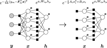
Figure 1: Left: Factor graph representation of the posterior (1) given the RBM signal prior (8). Circles and squares represent variables and factors, respectively. Light gray circles are the observed signal measurements. Black factors are the factors induced by linear operators $\mathbf{F}$ and $\mathbf{W}$. Light gray factors represent prior distributions influencing their adjoining variables. Right: Factor graph for the approximating posterior (2). Factors on the left represent local effective potentials provided by AMP at each of its iterations.

III TAP Approximation of a General-case RBM

In order to use the RBM model (8) as a prior within AMP, we must perform inference over the RBM graphical model given on the right of Fig. 1. Specifically, we construct a message-passing scheme between the factors and the hidden and visible variables of the RBM. Loopy BP has been considered in the context of inference on RBMs in [27], where the authors assume a Bernoulli distribution on the hidden variables and rewrite them as factors. In contrast, we investigate a more general setting with arbitrary distributions on both the hidden and visible variables. Since all factors have degree 2, using BP we can write the messages from variable to variable,

$$\psi_{i\rightarrow\mu}(x_{i}) =\frac{1}{\mathcal{Z}_{i\rightarrow\mu}}P_{0}(x_{i})e^{-\frac{1}{2}A_{i}^{\rm AMP}x_{i}^{2}+B_{i}^{\rm AMP}x_{i}}$$

$$\quad\quad\times\prod_{\nu\in\partial i/\mu}\int{\rm d}h_{\nu}~{}~{}\psi_{\nu\rightarrow i}(h_{\nu})e^{x_{i}W_{i\nu}h_{\nu}},$$ (10)

$$\psi{{}_{\mu\rightarrow i}}(h_{\mu}) =\frac{1}{\mathcal{Z}_{\mu\rightarrow i}}P_{0}(h_{\mu})$$

$$\quad\quad\times\prod_{j\in\partial\mu/i}\int{\rm d}x_{j}~{}~{}\psi_{j\rightarrow\mu}(x_{j})e^{x_{j}W_{j\mu}h_{\mu}},$$ (11)

where we index hidden units by $\mu$, $\nu$ and visible units by $i$, $j$, and the notation $\partial i/\mu$ represents the set of all edge-connected neighbors of variable $i$ except $\mu$. If we assume that the magnitudes of the values of $\mathbf{W}$ are small, then we can perform an expansion on the messages [15]. This is in essence the relaxed BP of [11], transitioning from messages of continuous distributions to messages parameterized by their first two central moments, denoted by the letters $a$ and $c$, respectively. Specifically,

$$\int{\rm d}h_{\nu}~{}~{}\psi_{\nu\rightarrow i}(h_{\nu})e^{x_{i}W_{i\nu}h_{\nu}}$$

$$~{}={\rm exp}\left\{x_{i}W_{i\nu}a^{\rm h}_{\nu\rightarrow i}+\frac{1}{2}x_{i}^{2}W_{i\nu}^{2}c^{\rm h}_{\nu\rightarrow i}\right\}+O(\mathbf{W}^{3}),$$ (12)

$$\int{\rm d}x_{j}~{}~{}\psi_{j\rightarrow\mu}(x_{j})e^{x_{j}W_{j\mu}h_{\mu}}$$

$$~{}={\rm exp}\left\{h_{\mu}W_{j\mu}a^{\rm v}_{j\rightarrow\mu}+\frac{1}{2}h_{\mu}^{2}W_{j\mu}^{2}c^{\rm v}_{j\rightarrow\mu}\right\}+O(\mathbf{W}^{3}),$$ (13)

where $O(\mathbf{W}^{3})$ represents a vanishing third-order correction to the two-moment approximation of the message marginalizations which is dependent on the RBM parameters $\mathbf{W}$. As we are now able to move the product of incoming messages as a sum into the exponent, we define the following intermediate sum variables as in AMP,

$$A^{\rm v}_{i\rightarrow\mu}\triangleq-\sum_{\nu\in H/\mu}W_{i\nu}^{2}c^{\rm h}_{\nu\rightarrow i},~{} B^{\rm v}_{i\rightarrow\mu}\triangleq\sum_{\nu\in H/\mu}W_{i\nu}a^{\rm h}_{\nu\rightarrow i},$$ (14)

$$A^{\rm h}_{\mu\rightarrow i}\triangleq-\sum_{j\in V/i}W_{j\mu}^{2}c^{\rm v}_{j\rightarrow\mu},~{} B^{\rm h}_{\mu\rightarrow i}\triangleq\sum_{j\in V/i}W_{j\mu}a^{\rm v}_{j\rightarrow\mu},$$ (15)

where the sets $H$ and $V$ are the set of all hidden and visible variables, respectively. From these definitions, we can define the message moments explicitly and close the message passing equations on the edges of the RBM factor graph,

$$a^{\rm h}_{\mu\rightarrow i} =f_{\rm a}^{\rm h}(A^{\rm h}_{\mu\rightarrow i},B^{\rm h}_{\mu\rightarrow i}), c^{\rm h}_{\mu\rightarrow i}=f_{\rm c}^{\rm h}(A^{\rm h}_{\mu\rightarrow i},B^{\rm h}_{\mu\rightarrow i}),$$ (16)

$$a^{\rm v}_{i\rightarrow\mu} =f_{\rm a}^{\rm v}(A_{i}^{\rm AMP}+A^{\rm v}_{i\rightarrow\mu},\, B_{i}^{\rm AMP}+B^{\rm v}_{i\rightarrow\mu}),$$ (17)

$$c^{\rm v}_{i\rightarrow\mu} =f_{\rm c}^{\rm v}(A_{i}^{\rm AMP}+A^{\rm v}_{i\rightarrow\mu},\, B_{i}^{\rm AMP}+B^{\rm v}_{i\rightarrow\mu}),$$ (18)

where the prior-dependent functions for the visible and hidden variables, $(f_{\rm a}^{\rm v},f_{\rm c}^{\rm v})$ and $(f_{\rm a}^{\rm h},f_{\rm c}^{\rm h})$ respectively, are defined in a fashion similar to (7), i.e. as the moments of an approximating distribution similar to (2), but using the desired hidden and visible distributions in place of $P_{0}$. The marginal beliefs at each hidden and visible variable can be defined by summing over all incoming messages. One could run this message passing, as stated, until convergence on the beliefs in order to infer marginal distributions on both the hidden and visible variables of the RBM. The moments of the marginal distributions on the visible units, $a_{i}^{\rm v}$ and $c_{i}^{\rm v}$, would give us exactly the moments required by the AMP iteration.

However, such a message passing on the edges of the factor graph can be quite memory and computationally intensive, especially if this inference occurs nested as an inner loop of AMP. If we assume that the entries of $\mathbf{W}$ are widely distributed, without any particular strong correlations in its structure, we can construct an algorithm which operates entirely on the beliefs, the nodes of the factor graph, rather than the messages, the edges. Such an algorithm is similar in spirit to AMP and also to the Thouless-Anderson-Palmer (TAP) equations from statistical physics. We now write these TAP self-consistency equations closed on the parameters of the marginal beliefs alone,

$$A_{\mu}^{\rm h} =-\sum_{i\in V}W_{i\mu}^{2}c_{i}^{\rm v},~{} B_{\mu}^{\rm h}=a_{\mu}^{\rm h}A_{\mu}^{\rm h}+\sum_{i\in V}W_{i\mu}a_{i}^{\rm v},$$ (19)

$$a_{\mu}^{\rm h} =f_{\rm a}^{\rm h}(A_{\mu}^{\rm h},B_{\mu}^{\rm h}),~{} c_{\mu}^{\rm h}=f_{\rm c}^{\rm h}(A_{\mu}^{\rm h},B_{\mu}^{\rm h}),$$ (20)

$$A_{i}^{\rm v} =-\sum_{\mu\in H}W_{i\mu}^{2}c_{\mu}^{\rm h},~{} B_{i}^{\rm v}=a_{i}^{\rm v}A_{i}^{\rm v}+\sum_{\mu\in H}W_{i\mu}a_{\mu}^{\rm h},$$ (21)

$$a_{i} =f_{\rm a}^{\rm v}(A_{i}^{\rm AMP}+A_{i}^{\rm v}\!,\, B_{i}^{\rm AMP}+B_{i}^{\rm v}),$$ (22)

$$c_{i} =f_{\rm c}^{\rm v}(A_{i}^{\rm AMP}+A_{i}^{\rm v}\!,\, B_{i}^{\rm AMP}+B_{i}^{\rm v}).$$ (23)

IV Implementation

Using the equations detailed in (19)–(23), we can construct a fixed-point iteration (FPI) which, given some arbitrary starting condition, can be run until convergence in order to obtain the GRBM-inferred distribution on the signal variables defined by $\mathbf{a}$, $\mathbf{c}$. These distributions are then passed back to the CS observational factors to complete the AMP iteration for CS reconstruction. We detail this procedure in Alg. 1. One important addition is the use of a damping step [28] on the RBM-inferred values of $\mathbf{a}$ and $\mathbf{c}$. We find that a fixed value of $\gamma=0.5$, equally combining the previous and presently inferred moments, stabilizes the interaction between the GRBM and the outer AMP inference. This becomes especially important for $\alpha$ small, where oscillations between the two inference loops degrades reconstruction performance.

Algorithm 1 AMP with GRBM Signal Prior

  Input: $\mathbf{F}$, $\mathbf{y}$, $\mathbf{W}$, $\theta^{\rm v}$, $\theta^{\rm h}$

  Initialize: $\mathbf{a}$,$\mathbf{c}$, ${\rm t}=1$ Outer AMP Inference Loop:

  repeat

     AMP Update on $\{V_{m},\omega_{m}\}$ as in (3), (4)

     AMP Update on $\{A_{i}^{\rm AMP},B_{i}^{\rm AMP}\}$ as in (5), (6)

     (Re)Initialize: $a_{i}=f_{\rm a}^{\rm v}(A_{i}^{\rm AMP},B_{i}^{\rm AMP})\;\forall i$, $a_{\mu}^{\rm h}=c_{\mu}^{\rm h}=0\;\forall\mu$ Inner RBM Inference Loop:

     repeat

        Update $\{A_{i}^{\rm v},B_{i}^{\rm v}\}$ as in (21)

        Update $\{a_{i},c_{i}\}$ as in (22), (23)

        Update $\{A_{\mu}^{\rm h},B_{\mu}^{\rm h}\}$ as in (19)

        Update $\{a_{\mu}^{\rm h},c_{\mu}^{\rm h}\}$ as in (20)

     until Convergence

     $\mathbf{a}^{(\rm t)}=\gamma\cdot\mathbf{a}^{(\rm t-1)}+(1-\gamma)\cdot\mathbf{a}$

     $\mathbf{c}^{(\rm t)}=\gamma\cdot\mathbf{c}^{(\rm t-1)}+(1-\gamma)\cdot\mathbf{c}$

     ${\rm t}\leftarrow{\rm t}+1$

  until Convergence on $\mathbf{a}$

While the Hamiltonian for the RBM model used here is in agreement with the literature on real-valued RBMs, the TAP FPI on the RBM points out one flaw in the construction of the real-valued RBM model. Specifically, the unbounded nature of the energy for variables in $\mathbb{R}$ manifests in this context by allowing negative variance-like terms $A_{i}^{\rm v}$ and $A_{\mu}^{\rm h}$ which carry through into the prior-dependent functions. We propose to handle this dilemma of negative variance by forcing the truncation of $P_{0}(h_{\mu})$ and $P_{0}(x_{i})$. Truncation can gracefully handle negative variances by transforming these distributions to uniformity over the truncation bounds. In practice, truncation is an easy assumption to make on both the training data and the signal to be reconstructed. For example, image data naturally lies within a specific range of values as defined by the images’ bit-depth. For sparse signals, such as those commonly studied in the context of CS, we propose the use of a truncated Gauss-Bernoulli distribution on the visible units, which only has non-zero probability density within a fixed range.

V Experiments

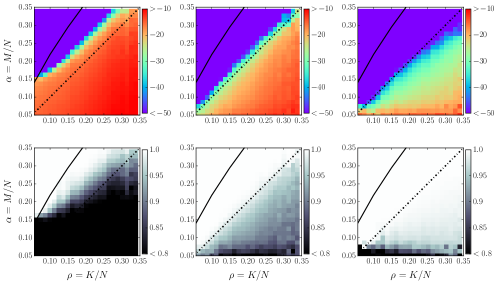
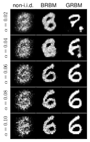
Figure 2: (Left) CS reconstruction performance over first 1,000 digit images from the MNIST test partition. Results for non-i.i.d. AMP, support-based BRBM-AMP, and GRBM-AMP are on the left, center, and right, respectively. The $M=K$ oracle support transition is indicated by the black dotted line, and the spinodal transition [15] by the solid one. Top: Average reconstruction accuracy in MSE measured in dB. Bottom: Average reconstruction correlation with original digit image. (Right) Visual comparison of reconstructions for a single digit image ($\rho=0.25$) for small values of $\alpha$.

We now present the results of our numerical studies of GRBM-AMP performance for the AWGN CS reconstruction task. For all reconstruction tasks, an AWGN noise variance $\Delta=10^{-8}$ was used. Additionally, all elements of the sampling matrices $\mathbf{F}$ were drawn from a zero-mean Gaussian distribution of variance $1/\sqrt{N}$.

The results we present are based on the MNIST handwritten digit dataset [29] which consists of $28\times 28$ gray-scale digit images split between 60,000 training samples and 10,000 test samples. While we train over the entire MNIST training partition, we conduct our reconstruction experiments for the first 1,000 digit images drawn from the test partition. We test three different approaches for this dataset. The first, termed non-i.i.d. AMP, consists of empirically estimating the per-coefficient prior hyper-parameters from the training data. This approach assumes a fully factorized model of the data, neglecting any covariance structure between the coefficients. The second approach is that of [18], here termed binary-support RBM (BRBM-AMP), which uses a binary RBM to model the correlation structure of the support, alone. Finally, we test the proposed GRBM-AMP, using a general RBM trained with binary hidden units and Gauss-Bernoulli visible units, which models the data in its ambient domain.

To train the GRBM parameters for MNIST, we use a GRBM with 784 binary hidden units. The RBM can be trained using either contrastive divergence, sampling the visible units from a truncated GB prior, or using the GRBM TAP iteration shown here in conjunction with the EMF strategy of [24], a strategy which we detail in a forthcoming work. For the specific GRBM model we use for these CS experiments, we train a GRBM using the EMF approach for 150 epochs using a learning rate of 0.01 with an $\ell_{2}$ weight decay penalty of 0.001. Learning momentum of 0.5 was used. Finally, the truncation bounds were set to the range $[0,1]$. In the case of the BRBM, where all variables are binary, EMF training [24] was used with a learning rate of 0.005, while other parameters have been set the same as for the GRBM.

We present the results of the three approaches in Fig. 2, where we evaluate reconstruction performance over the test set in terms of both MSE, measured in decibels, and correlation between the reconstructed and original images, where correlation is measured as $(\mathbf{x}-\bar{x})^{T}(\mathbf{a}-\bar{a})/\sigma_{\mathbf{x}}\sigma_{\mathbf{a}}$. In both of these comparisons, we show performance over the phase diagram, where $\alpha$ refers to the number of CS measurements observed and $\rho$ refers to the overall sparsity for each digit image, $K/N$, where $K$ is the number of non-zero pixels in the digit image. As many of the tested images posses few non-zeros, the test dataset is skewed towards small $\rho$, hence the increased variability at $\rho>0.3$ for Fig. 2. From these results, we can see a clear progression of reconstruction performance as we move from an empirical factorized model, to a model of the support alone, to a model of the signal itself. For non-i.i.d. AMP, we see that the localized information from the training set allows for a transition curve which is parallel to $M=K$, which is in contrast to the well-known transition for AMP with an i.i.d. GB signal prior. For BRBM-AMP we observe that the reconstruction transition lies very close to the $M=K$ optimal line, as also observed in [18], showing the advantage of leveraging the strong support correlations which exist in the dataset. In the case of the GRBM-AMP, we observe that the maximal performance is no longer bounded by the $M=K$ line, with low MSE achievable even for $M<K$. This is an intuitive result, as the GRBM model provides information not only about the support, but also about the values of the signal on that support. This effect is most drastically observed in terms of the average reconstruction correlation, where we observe almost perfect correlation for the entire test set for $\alpha>0.10$, independent of the signal sparsity.

Finally, we also see a visual comparison for one example of a reconstructed digit in Fig. 2 in the small $\alpha$ setting. In this extreme case, we can see that both the BRBM- and GRBM-AMP produce reconstructions whose support closely match the original ‘6’ digit image. We note that the GRBM is able to capture the smoothness of the digit image where the BRBM cannot.

VI Conclusion

In this work, we derived an AMP-based algorithm for CS signal reconstruction using an RBM to model the signal class in its ambient domain. To accomplish this modeling, we developed a model for a class of general RBMs, allowing for arbitrary distributions on the hidden and visible units. To allow the use of such a model within AMP, we proposed a TAP-based approximation of the RBM which we derived from belief propagation. By performing inference on the RBM under the influence of the outer AMP inference, we have developed a novel algorithm for CS reconstruction of sparse structured data. The proposed approach can be of great use in signal reconstruction contexts where there exists an abundance of data which lack developed correlation models. Additionally, the inference we propose for general RBMs could be used to develop novel generative models by varying its architecture and the distribution of the hidden variables.

References

- [1] E. J. Candès and M. B. Wakin, “An introduction to compressive sampling,” IEEE Signal Processing Magazine, vol. 25, no. 2, pp. 21–30, 2008.
- [2] E. Candès and J. Romberg, “Signal recovery from random projections,” in Computational Imaging III. Proc. SPIE 5674, Mar. 2005, pp. 76–86.
- [3] D. L. Donoho, “Compressed sensing,” IEEE Trans. on Information Theory, vol. 52, no. 4, pp. 1289–1306, Apr. 2006.
- [4] D. Takhar, J. N. Laska, M. B. Wakin, M. F. Duarte, D. Baron, S. Sarvotham, K. F. Kelly, and R. G. Baraniuk, “A new compressive imaging camera architecture using optical-domain compression,” in Computational Imaging IV. Proc. SPIE 6065, 2006, p. 606509.
- [5] M. Mishali, Y. C. Eldar, O. Dounaevsky, and E. Shoshan, “Xampling: Analog to digital at sub-Nyquist rates,” IET Circuits, Devices and Systems, vol. 5, no. 1, pp. 8–20, January 2011.
- [6] Z. Zhang, Y. Xu, J. Yang, X. Li, and D. Zhang, “A survey of sparse representation: Algorithms and applications,” IEEE Access, vol. 3, pp. 290–530, 2015.
- [7] D. L. Donoho, Y. Tsaig, I. Drori, and J.-L. Starck, “Sparse solution of underdetermined linear equations by stagewise orthogonal matching pursuit,” Stanford University, Tech. Rep., 2006.
- [8] T. T. Do, L. Gan, N. Nguyen, and T. D. Tran, “Sparsity adaptive matching pursuit algorithm for practical compressed sensing,” in Proc. Asilomar Conf. on Signals, Systems, and Computers, Pacific Grove, California, Oct. 2008, pp. 581–587.
- [9] D. L. Donoho and J. Tanner, “Thresholds for the recovery of sparse solutions via l1 minimization,” in Information Sciences and Systems, Proc. Annual Conference on, 2006, pp. 202–206.
- [10] D. Baron, S. Sarvotham, and R. G. Baraniuk, “Bayesian compressive sensing via belief propagation,” IEEE Trans. on Signal Processing, vol. 58, no. 1, pp. 269–280, 2009.
- [11] S. Rangan, “Estimation with random linear mixing, belief propagation and compressed sensing,” in Proc. Annual Conf. on Information Sciences and Systems, 2010, pp. 1–6.
- [12] D. L. Donoho, A. Maleki, and A. Montanari, “Message-passing algorithms for compressed sensing,” Proc. Nat. Academy of Sciences of the U.S.A., vol. 106, no. 45, p. 18914, 2009.
- [13] ——, “Message passing algorithms for compressed sensing: II. analysis and validation,” in Proc. IEEE Info. Theory Workshop, Cairo, Egypt, 2010, pp. 1–5.
- [14] S. Rangan, “Generalized approximate message passing for estimation with random linear mixing,” in Proc. IEEE Intl. Symp. on Info. Theory, 2011, p. 2168.
- [15] F. Krzakala, M. Mézard, F. Sausset, Y. Sun, and L. Zdeborová, “Probabilistic reconstruction in compressed sensing: Algorithms, phase diagrams, and threshold achieving matrices,” Journal of Statistical Mechanics: Theory and Experiment, vol. 2012, no. 8, p. P08009, 2012.
- [16] ——, “Statistical physics-based reconstruction in compressed sensing,” Phys. Rev. X, vol. 2, p. 021005, 2012.
- [17] A. Drémeau, C. Herzet, and L. Daudet, “Boltzmann machine and mean-field approximation for structured sparse decompositions,” IEEE Trans. on Signal Processing, vol. 60, no. 7, pp. 3425–3438, 2012.
- [18] E. W. Tramel, A. Drémeau, and F. Krzakala, “Approximate message passing with restricted Boltzmann machine priors,” Journal of Statistical Mechanics: Theory and Experiment, 2016, to appear.
- [19] K. Kulkarni, S. Lohit, P. Turaga, R. Kerviche, and A. Ashok, “ReconNet: Non-iterative reconstruction of images from compressively sensed random measurements,” 2016, arXiv:1601.06892.
- [20] A. Mousavi, A. B. Patel, and R. G. Baraniuk, “A deep learning approach to structured signal recovery,” 2015, arXiv:1508.04065.
- [21] U. S. Kamilov and H. Mansour, “Learning optimal nonlinearities for iterative thresholding algorithms,” 2015, arXiv:1512.04754.
- [22] P. Schniter, “Turbo reconstruction of structured sparse signals,” in Proc. Conf. on Info. Sciences and Systems, 2010, pp. 1–6.
- [23] S. Rangan, A. K. Fletcher, V. K. Goyal, and P. Schniter, “Hybrid approximate message passing with applications to structured sparsity,” 2011, arXiv:1111.2581.
- [24] M. Gabrié, E. W. Tramel, and F. Krzakala, “Training restricted Boltzmann machines via the Thouless-Andreson-Palmer free energy,” in Advances in Neural Information Processing System, vol. 28, Montreal, Canada, June 2015, pp. 640–648.
- [25] P. Smolensky, Information Processing in Dynamical Systems: Foundations of Harmony Theory, ser. Parallel Distributed Porcessing: Explorations in the Microsctructure of Cognition. MIT Press, 1986, ch. 6, pp. 194–281.
- [26] G. E. Hinton, “Training products of experts by minimizing contrastive divergence,” Neural Computation, vol. 14, no. 8, pp. 1771–1800, 2002.
- [27] H. Huang and T. Toyoizumi, “Advanced mean-field theory of restricted Boltzmann machine,” Physical Review E, vol. 91, no. 5, p. 050101, 2015.
- [28] T. Heskes, “Stable fixed points of loopy belief propagation are minima of the Bethe free energy,” in Advances in Neural Information Processing Systems, vol. 15, 2002, pp. 359–366.
- [29] Y. LeCun, L. Bottu, Y. Bengio, and P. Haffner, “Gradient-based learning applied to document recognition,” Proc. of the IEEE, vol. 86, no. 11, pp. 2278–2324, November 1998.