Topological entanglement negativity in Chern-Simons theories
Xueda Wen ¹, Po-Yao Chang ², and Shinsei Ryu ¹

¹Institute for Condensed Matter Theory and Department of Physics, University of Illinois at Urbana-Champaign, 1110 West Green St, Urbana IL 61801, USA

²Center for Materials Theory, Rutgers University, Piscataway, NJ, 08854, USA

We study the topological entanglement negativity between two spatial regions in (2+1)-dimensional Chern-Simons gauge theories by using the replica trick and the surgery method. For a bipartitioned or tripartitioned spatial manifold, we show how the topological entanglement negativity depends on the presence of quasiparticles and the choice of ground states. In particular, for two adjacent non-contractible regions on a tripartitioned torus, the entanglement negativity provides a simple way to distinguish Abelian and non-Abelian theories. Our method applies to a Chern-Simons gauge theory defined on an arbitrary oriented (2+1)-dimensional spacetime manifold. Our results agree with the edge theory approach in a recent work (X. Wen, S. Matsuura and S. Ryu, arXiv:1603.08534).

1 Introduction

Recently, quantum entanglement provides a powerful tool to study the properties of quantum many-body systems in condensed matter physics [2, 3, 4, 5], such as characterizing topological ordered phases, and detecting the central charge of conformal field theories, etc. [2, 3, 4, 5, 6, 7, 8].

To characterize the quantum entanglement, there are various kinds of entanglement measures. In the case when a system is prepared in a pure state $|\Psi\rangle$ and bipartitioned into two subsystems $A$ and $B$, two quantum entanglement measures which turn out to be very useful are the so-called Renyi entropy and von Neumann entropy defined as follows

$$S_{A}^{(n)}=\frac{1}{1-n}\ln\text{Tr}\rho_{A}^{n},\quad\text{and}\quad S_{A}^{\text{vN}}=-\text{Tr}\rho_{A}\ln\rho_{A},$$ (1.1)

where $n$ is an integer, and $\rho_{A}=\text{Tr}_{B}\rho$ is the reduced density matrix of subsystem $A$, with $\rho=|\Psi\rangle\langle\Psi|$. The Renyi entropy and von Neumann entropy are related by $S_{A}^{\text{vN}}=\lim_{n\to 1}S_{A}^{(n)}$. It is noted that when $\rho$ corresponds to a pure state, one has the nice property that $S_{A}^{(n)}=S_{B}^{(n)}$ and $S_{A}^{\text{vN}}=S_{B}^{\text{vN}}$. For a mixed state, it is found that the quantum and classical correlations cannot be explicitly separated in these entanglement measures. Now we consider two subsystems $A_{1}$ and $A_{2}$ which are embedded in a larger system, and therefore $\rho_{A_{1}\cup A_{2}}$ may correspond to a mixed state. In this case, a useful quantity to study the correlation between $A_{1}$ and $A_{2}$ is the Renyi mutual information

$$I_{A_{1}A_{2}}^{(n)}=S_{A_{1}}^{(n)}+S_{A_{2}}^{(n)}-S_{A_{1}\cup A_{2}}^{(n)},$$ (1.2)

which is symmetric in $A_{1}$ and $A_{2}$ by definition. Similar to the von Neumann entropy, by taking the $n\to 1$ limit, one can obtain the (von Neumann) mutual information

$$I_{A_{1}A_{2}}=\lim_{n\to 1}I_{A_{1}A_{2}}^{(n)}.$$ (1.3)

It is found that the mutual information will mix the quantum and classical information together [9], and hence is not a good entanglement measure for mixed states.

Another quantity under extensive study, which is useful in characterizing the quantum entanglement in mixed states, is the entanglement negativity [10, 11]. To be concrete, for a reduced density matrix $\rho_{A_{1}A_{2}}$ which describes a mixed state in the Hilbert space $\mathcal{H}_{A_{1}}\otimes\mathcal{H}_{A_{2}}$, a partial transposition of $\rho_{A_{1}A_{2}}$ with respect to the degrees of freedom in region $A_{2}$ is defined as

$$\langle e_{i}^{(1)}e_{j}^{(2)}|\rho_{A_{1}\cup A_{2}}^{T_{2}}|e_{k}^{(1)}e_{l}^{(2)}\rangle=\langle e_{i}^{(1)}e_{l}^{(2)}|\rho_{A_{1}\cup A_{2}}|e_{k}^{(1)}e_{j}^{(2)}\rangle,$$ (1.4)

where $T_{2}$ represents the partial transposition over $A_{2}$, $|e_{i}^{(1)}\rangle$ and $|e_{j}^{(2)}\rangle$ are arbitrary bases in $\mathcal{H}_{A_{1}}$ and $\mathcal{H}_{A_{2}}$, respectively. Then the entanglement negativity is defined as

$$\mathcal{E}_{A_{1}A_{2}}:=\ln\text{tr}\left|\rho_{A_{1}\cup A_{2}}^{T_{2}}\right|.$$ (1.5)

To calculate the entanglement negativity in a quantum filed theory, it is convenient to use the replica trick as follows [12, 13]

$$\mathcal{E}_{A_{1}A_{2}}=\lim_{n_{e}\to 1}\ln\text{tr}\left(\rho_{A_{1}\cup A_{2}}^{T_{2}}\right)^{n_{e}},$$ (1.6)

where $n_{e}$ is an even integer.

Recently, the entanglement negativity has been extensively studied in conformal field theories [12, 13, 14], quantum spin chain systems [15, 16], coupled harmonic oscillators in one and two dimensions [17, 18, 19], free fermion systems [20, 21, 22, 23], topological ordered systems [24, 25, 26], and holographic entanglement [27, 28, 29]. Furthermore, the entanglement negativity has also been studied in the non-equilibrium case [30, 31, 32, 33] as well as the finite temperature case [30, 34, 35].

In this work, we focus on the topological entanglement negativity in a particular topological quantum field theory (TQFT)–the Chern-Simons theory [39, 40]. TQFTs are extensively used in condensed matter physics because of the emergence of topological phases from many-body systems such as the fractional quantum Hall states [36], gapped quantum spin liquids [37], $p_{x}+ip_{y}$ superconductors [38] and so on. It is noted that the entanglement negativity for a toric code model, an Abelian topological ordered system, has been studied in previous works [24, 25]. Later, an edge theory approach was developed to study the entanglement negativity (and other entanglement measures) in a Chern-Simons theory. Due to the bulk-boundary correspondence in a Chern-Simons theory, we present an alternative approach to study the entanglement negativity from bulk point of view. By applying the replica trick and the surgery method [39, 6], we compute the entanglement negativity in a generic Chern-Simons theory.

The rest of the paper is organized as follows. In Sec. 1.1, we introduce the path integral representation of a partially transposed reduced density matrix, which is used to define the entanglement negativity. In Sec. 1.2, we introduce the basic ingredients of Chern-Simons theory and the surgery method. Then by using the surgery method and the replica trick, we calculate the entanglement negativity on various bi-/tri-partitioned manifolds for a Chern-Simons theory in Sec.2, and study how the entanglement negativity depends on the presence of quasiparticles and the choice of ground states. Then we conclude in Sec. 3. We also include several appendices containing the calculation of the entanglement negativity for a bipartitioned torus, which is helpful to understand the case of a tripartite torus in the main text. To compare with the entanglement negativity, we also calculate the mutual information for various cases in the appendices.

1.1 Path integral representation of partially transposed reduced density matrix

In this section, we introduce the path integral representation of a partially transposed reduced density matrix, i.e., $\rho_{A_{1}\cup A_{2}}^{T_{2}}$ [see Eq. (1.4)], as well as $\text{tr}\left(\rho_{A_{1}\cup A_{2}}^{T_{2}}\right)^{n_{e}}$ [see Eq. (1.6)]. The definition in this part applies to a generic quantum field theory.

The density matrix in a thermal state can be expressed as a path integral in the imaginary time interval $(0,\beta)$ [8, 13]

$$\rho\Big{[}\{\varphi_{0}(\vec{x})\},\{\varphi_{\beta}(\vec{x})\}\Big{]} =\frac{1}{Z(\beta)}\left\langle\{\varphi_{0}(\vec{x})\}|e^{-\beta H}|\{\varphi_{\beta}(\vec{x})\}\right\rangle$$

$$=\int\prod[d\phi(\vec{x},\tau)]e^{-S_{E}}\prod_{\vec{x}}\delta[\phi(\vec{x},0)-\varphi_{0}(\vec{x})]\delta[\phi(\vec{x},\beta)-\varphi_{\beta}(\vec{x})],$$ (1.7)

with $\beta\to\infty$ corresponding to the zero temperature limit. Here $S_{E}$ is the Euclidean action and $Z=\text{tr}e^{-\beta H}$ is the partition function. $\vec{x}$ represents the coordinate in the $d$-dimensional space, and $\tau$ is the imaginary time. The rows and columns of the density matrix are represented by the values of fields $\phi(\vec{x},\tau)$ at $\tau=0$ and $\beta$, respectively. Now we take partial transposition corresponding to a subsystem $B$, then the partial transposed density matrix may be expressed as

$$\quad\rho^{T_{B}}\Big{[}\{\varphi_{0}(\vec{x})\},\{\varphi_{\beta}(\vec{x})\}\Big{]} =\int\prod_{\vec{x},\tau}[d\phi(\vec{x},\tau)]e^{-S_{E}}\prod_{\vec{x}\notin B}\delta[\phi(\vec{x},0)-\varphi_{0}(\vec{x})]\delta[\phi(\vec{x},\beta)-\varphi_{\beta}(\vec{x})]$$

$$\quad\times\prod_{\vec{x}\in B}\delta[\phi(\vec{x},0)-\varphi_{\beta}(\vec{x})]\delta[\phi(\vec{x},\beta)-\varphi_{0}(\vec{x})].$$ (1.8)

Suppose the system is tripartitioned into $A_{1}$, $A_{2}$ and $B$, then the reduced density matrix for $\rho_{A=A_{1}\cup A_{2}}$ can be obtained by tracing $B$, i.e.,

$$\rho_{A_{1}\cup A_{2}}\left[\{\varphi_{0}(\vec{x})\},\{\varphi_{\beta}(\vec{x})\}\Big{|}\vec{x}\in A_{1}\cup A_{2}\right]$$

$$=\int\left(\prod_{\vec{x}\in B}[d\varphi_{0}(\vec{x})d\varphi_{\beta}(\vec{x})]\delta[\varphi_{0}(\vec{x})-\varphi_{\beta}(\vec{x})]\right)\rho\Big{[}\{\varphi_{0}(\vec{x})\},\{\varphi_{\beta}(\vec{x})\}\Big{]}.$$ (1.9)

Then the partial transposed reduced density matrix $\rho_{A_{1}\cup A_{2}}^{T_{2}}$ over the subregion $A_{2}$ may be expressed as

$$\quad\rho_{A_{1}\cup A_{2}}^{T_{A_{2}}}\left[\{\varphi_{0}(\vec{x})\},\{\varphi_{\beta}(\vec{x})\}\Big{|}\vec{x}\in A_{1}\cup A_{2}\right]$$

$$=\int\left(\prod_{\vec{x}\in B}[d\varphi_{0}(\vec{x})d\varphi_{\beta}(\vec{x})]\delta[\varphi_{0}(\vec{x})-\varphi_{\beta}(\vec{x})]\right)\rho^{T_{A_{2}}}\Big{[}\{\varphi_{0}(\vec{x})\},\{\varphi_{\beta}(\vec{x})\}\Big{]}.$$ (1.10)

Then, $\text{tr}\left(\rho_{A_{1}\cup A_{2}}^{T_{A_{2}}}\right)^{n}$ can be obtained by taking $n$ copies of $\rho_{A_{1}\cup A_{2}}^{T_{A_{2}}}$, and glue them appropriately as follows

$$\quad\text{tr}\left(\rho_{A_{1}\cup A_{2}}^{T_{A_{2}}}\right)^{n}=\int\prod_{k=1}^{n}\Bigg{\{}\prod_{\vec{x}}\left[d\varphi_{0}^{(k)}(\vec{x})d\varphi_{\beta}^{(k)}(\vec{x})\right]\prod_{\vec{x}\in B}\delta\left[\varphi_{0}^{(k)}(\vec{x})-\varphi_{\beta}^{(k)}(\vec{x})\right]$$

$$\times\prod_{\vec{x}\in A_{1}}\delta\left[\varphi_{0}^{(k)}(\vec{x})-\varphi_{\beta}^{(k+1)}(\vec{x})\right]\prod_{\vec{x}\in A_{2}}\delta\left[\varphi_{\beta}^{(k)}(\vec{x})-\varphi_{0}^{(k+1)}(\vec{x})\right]\rho\left[\{\varphi_{0}^{(k)}(\vec{x})\},\{\varphi_{\beta}^{(k)}(\vec{x})\}\right]\Bigg{\}},$$ (1.11)

with $i\equiv i$ mod $n$. As a comparison, it should be noted that $\text{tr}\left(\rho_{A_{1}\cup A_{2}}\right)^{n}$ has the expression

$$\begin{split}\text{tr}\Big{(}\rho_{A_{1}\cup A_{2}}\Big{)}^{n}=&\int\prod_{k=1}^{n}\Bigg{\{}\prod_{\vec{x}}\left[d\varphi_{0}^{(k)}(\vec{x})d\varphi_{\beta}^{(k)}(\vec{x})\right]\prod_{\vec{x}\in B}\delta\left[\varphi_{0}^{(k)}(\vec{x})-\varphi_{\beta}^{(k)}(\vec{x})\right]\\ &\times\prod_{\vec{x}\in A}\delta\left[\varphi_{0}^{(k)}(\vec{x})-\varphi_{\beta}^{(k+1)}(\vec{x})\right]\rho\left[\{\varphi_{0}^{(k)}(\vec{x})\},\{\varphi_{\beta}^{(k)}(\vec{x})\}\right]\Bigg{\}}.\end{split}$$ (1.12)

Once we obtain $\text{tr}\left(\rho_{A_{1}\cup A_{2}}^{T_{A_{2}}}\right)^{n}$, we can calculate the entanglement negativity based on Eq. (1.6).

1.2 Chern-Simons theory and surgery

Here we mainly review the properties of Chern-Simons theory that will be used in our study of the entanglement negativity. One may refer to the seminal paper [39] for details of the Chern-Simons theory. The Chern-Simons theory action with a gauge group $G$ on a three-manifold $M$ is given by

$$S_{\text{CS}}=\frac{k}{4\pi}\int_{M}\text{tr}\left(A\wedge dA+\frac{2}{3}A\wedge A\wedge A\right),$$ (1.13)

where ‘tr’ is the trace over the fundamental representation of the gauge group $G$, $A$ is the $G$-connection on a genetic three-manifold $M$, and $k$ is the coupling constant, which is quantized. The Chern-Simons theory is a topological field theory in the sense that the correlation functions do not depend on the metric of the manifold $M$. Since the action of the Chern-Simons theory does not contain the metric, the partition function

$$Z(M)=\int[\mathcal{D}A]\mathrm{e}^{iS_{\text{CS}}(A)},$$ (1.14)

can define a topological invariant of the manifold $M$. Besides the partition function as an invariant of three-manifolds, invariants of links and knots in three-manifolds can be also defined in the Chern-Simons theory. Such a link or a knot in three-manifolds are the “Wilson line”, that traces the holonomy of the gauge connection on an oriented closed curve $\mathcal{C}$ in a given irreducible representation $\hat{R}$ of $G$,

$$W_{R}^{\mathcal{C}}(A)=\mathrm{tr}_{R}P\exp\int_{\mathcal{C}}A.$$ (1.15)

We can compute the correlation functions of non-intersecting links/knots $\mathcal{C}_{i}$, $i=1,\cdots,N$, with a representation $\hat{R}_{i}$ to each $\mathcal{C}_{i}$ on a three-manifold $M$,

$$Z(M,\hat{R}_{1},\cdots,\hat{R}_{N})=\langle W_{\hat{R}_{1}}^{\mathcal{C}_{1}}\cdots W_{\hat{R}_{N}}^{\mathcal{C}_{N}}\rangle=\int[\mathcal{D}A]\left(\prod_{i=1}^{N}W_{\hat{R}_{i}}^{\mathcal{C}_{i}}\right)\mathrm{e}^{iS_{\text{CS}}}.$$ (1.16)

(When necessary, we denote the partition function as $Z(M,[\hat{R}_{1},\cdots,\hat{R}_{N}]_{\mathcal{C}_{1},\cdots,\mathcal{C}_{N}})$ where $[\hat{R}_{1},\cdots,\hat{R}_{N}]_{\mathcal{C}_{1},\cdots,\mathcal{C}_{N}}$ indicates the configuration of the links/knots of Wilson loops.) These links/knots correlation functions can be seen as the partition functions of a Chern-Simons theory on a three-manifold $M$ in the presence of Wilson loops. As shown by Witten [39], the the partition functions are exactly calculable by canonical quantization and the surgery.

The key ingredient of computing the partition function is canonical quantization of a Chern-Simons theory on a three-manifold $M$ with boundary given by a Riemann surface $\Sigma$. This canonical quantization will produce a Hilbert space $\mathcal{H}_{\Sigma}$ with an associated state $|\Psi_{M}\rangle$. The dual Hilbert space $\mathcal{H}^{*}_{\Sigma}$ with an associated state $\langle\Psi_{M}|$ state can be obtained by reversing the orientation of the $\Sigma$. The partition function of a Chern-Simons theory on a (closed) three-manifold can be computed by performing the Heegaard splitting, which decomposes the three-manifold as the connected sum of two three-manifolds $M_{1}$ and $M_{2}$ with common boundary $\Sigma$. The original three-manifold $M=M_{1}\bigcup_{f}M_{2}$ is obtained by gluing $M_{1}$ and $M_{2}$ through their boundary under the homeomorphism $f:\Sigma\to\Sigma$. This homeomorphism acting in the Hilbert space can be presented by an operator $U_{f}:\mathcal{H}_{\Sigma}\to\mathcal{H}_{\Sigma}$. Hence the partition can be evaluated as

$$Z(M)=\langle\Psi_{M_{2}}|U_{f}|\Psi_{M_{1}}\rangle.$$ (1.17)

When the boundary is a sphere, i.e., $\Sigma=S^{2}$, the Hilbert space $\mathcal{H}_{S^{2}}$ is one dimensional. When the boundary $\Sigma=T^{2}$, which can be seen as the boundary of a solid torus $\mathbf{T}=D\times S^{1}$, one can obtain a state in $\mathcal{H}_{T^{2}}$ by inserting a Wilson loop in the representation $\hat{R}_{i}$ around the non-contractible cycle in the solid torus,

$$|\Psi_{\mathbf{T},\hat{R}_{i}}\rangle=|\hat{R}_{i}\rangle.$$ (1.18)

The state without the Wilson loop is the vacuum state, denoted as $|\hat{0}\rangle$.

The above results allow us to compute the partition function on three-manifolds in the presence of Wilson loops. Let us start with $S^{2}\times S^{1}$, which can be seen as gluing two solid tori ${\bf T}=D\times S^{1}$ with boundaries identified. I.e., $S^{2}$ comes from gluing two discs together along their boundary $S^{1}$. The partition function of a Chern-Simons theory in this three-manifold is

$$Z(S^{2}\times S^{1})=\langle\hat{0}|\hat{0}\rangle=1.$$ (1.19)

Performing the modular transformation $S$: $\tau\to-\frac{1}{\tau}$ on the second solid torus, where $\tau$ is the modular parameter of the torus, and gluing it back, i.e., the non-contractible cycle of the first solid torus is homologous to the contractible cycle of the second solid torus, we get $S^{3}$. We obtain the Chern-Simons partition function

$$Z(S^{3})=\langle\hat{0}|S|\hat{0}\rangle=\mathcal{S}_{00},$$ (1.20)

where $\mathcal{S}_{ij}$ is the element of the modular $\mathcal{S}$ matrix. If there is a Wilson loop in the representation $\hat{R}_{i}$ in one solid torus, the Chern-Simons partition functions become

$$Z(S^{2}\times S^{1},\hat{R}_{i})=\langle\hat{0}|\hat{R}_{i}\rangle=\delta_{0,i},$$

$$Z(S^{3},\hat{R}_{i})=\langle\hat{0}|S|\hat{R}_{i}\rangle=\mathcal{S}_{0i}.$$ (1.21)

One can also consider a Wilson loop in the representation $\hat{R}_{i}$ in a solid torus, which is glued to another solid torus with a Wilson loop in the representation $\hat{R}_{j}$. The Chern-Simons partition functions are

$$Z(S^{2}\times S^{1},\hat{R}_{i},\hat{R}_{j})=\langle\hat{R}_{i}|\hat{R}_{j}\rangle=\delta_{i,j}.$$

$$Z(S^{3},\hat{R}_{i},\hat{R}_{j})=\langle\hat{R}_{i}|S|\hat{R}_{j}\rangle=\mathcal{S}_{ij}.$$ (1.22)

Here we list two main properties of the above results:

1. The normalized vacuum expectation values of disjointed Wilson loops can be factorized, i.e.,

   $$\frac{Z(M,\hat{R}_{1},\cdots,\hat{R}_{N})}{Z(S^{3})}=\prod_{i=1}^{N}\frac{Z(M_{i},\hat{R}_{i})}{Z(S^{3})},$$ (1.23)

   where the three-manifold $M$ is the connected sum of $N$ three-manifolds $M_{i}$ joined along $N-1$ two spheres $S^{2}$. This result comes from the fact that the Hilbert space for $S^{2}$ is one-dimensional.

2. If Wilson loops are linked or they are passing through the common boundary $S^{2}$ between $M_{i}$ and $M_{j}$, the factorizability of the partition function is hold when the Hilbert space for $S^{2}$ with a pair of charges in the dual representations $\hat{R}_{i}$ and $\hat{\overline{R}}_{i}$ is one-dimensional. We have

   $$Z(M,[\blacksquare_{1},\blacksquare_{2},\hat{R}_{i},\hat{\overline{R}}_{i}]_{\mathcal{C}})\cdot Z(S^{3},\hat{R}_{i}) =Z(M_{1},[\blacksquare_{1},\hat{R}_{i}]_{\mathcal{C}_{1}})\cdot Z(M_{2},[\blacksquare_{2},\hat{R}_{i}]_{\mathcal{C}_{2}}),$$ (1.24)

   where $\blacksquare_{1(2)}$ contains Wilson loops with a general links/knots configuration $\mathcal{C}_{1(2)}$ in the shaded region in the $M_{1(2)}$ manifold shown in Fig. 1.

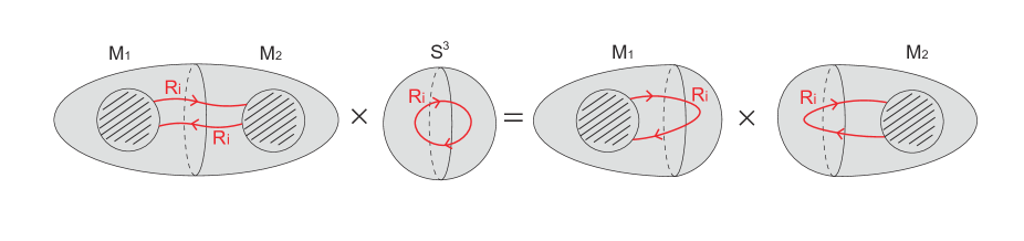
Figure 1: The surgery procedure to relate the partition function on a manifold $M_{1}\cup M_{2}$ with the partition functions on $M_{1}$ and $M_{2}$. The shaded region in $M_{1(2)}$ contains Wilson loops with a general links/knots configuration $\mathcal{C}_{1(2)}$.

A surgery procedure we will frequently use in this work is Eq. (1.24). We relate the partition function on a manifold $M_{1}\cup M_{2}$ with the partition functions on $M_{1}$ and $M_{2}$, by a factor $Z(S^{3},\hat{R}_{i})=\mathcal{S}_{0i}$. Notice that we do not consider any links/knots configuration of Wilson loops in our following discussion. This indicates in our discussion, $\blacksquare_{1(2)}$ in Eq. (1.24) only contains unlinked/unknoted Wilson loops.

In addition, the modular $\mathcal{S}$-matrix, which is unitary, is related with the quantum dimension as follows

$$d_{a}=\frac{\mathcal{S}_{0a}}{\mathcal{S}_{00}}.$$ (1.25)

The unitarity condition for the $\mathcal{S}$-matrix implies that

$$\left(\mathcal{S}_{00}\right)^{-1}=\sqrt{\sum_{i}|d_{i}|^{2}}=:\mathcal{D}.$$ (1.26)

2 Topological entanglement negativity

Based on the above discussion, we study the topological entanglement negativity between two spatial subregions on various manifolds in this section. The entanglement negativity is calculated in the following steps. (1) We consider $\text{tr}\left(\rho_{A_{1}\cup A_{2}}^{T_{2}}\right)^{n_{e}}$ as the partition function on a three-manifold $M$. (2) We use the surgery method to compute $\text{tr}\left(\rho_{A_{1}\cup A_{2}}^{T_{2}}\right)^{n_{e}}$, and then take $n_{e}\to 1$.

To avoid confusions, a spatial manifold is a two-manifold, which can be viewed as the boundary of the three-dimensional spacetime manifold where the wave function is defined.

2.1 Bipartition of a sphere

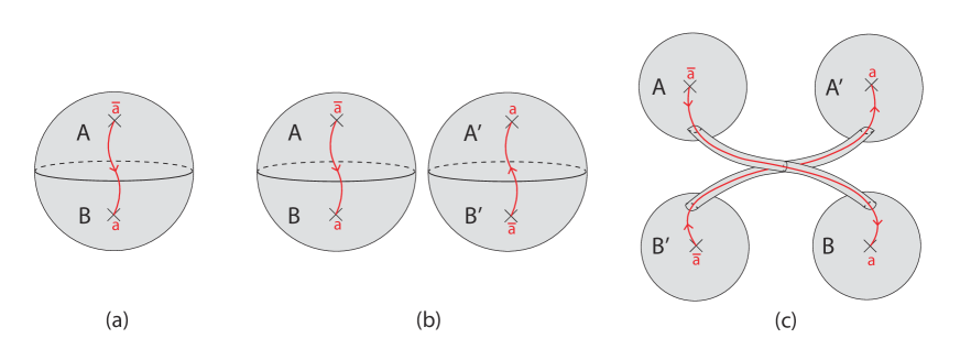
Figure 2: (a) Wave functional $|\Psi\rangle$. A Wilson line in representation $\hat{R}_{a}$ threads through the $AB$ interface. Shading implies a three-ball. (b) $\rho_{A\cup B}=|\Psi\rangle\langle\Psi|$. (c) $\rho_{A\cup B}^{T_{B}}$, in which we take partial transpose over $B$, i.e., we switch $B$ with $B^{\prime}$.

In this part, for the pedagogical purpose, we consider the simplest case, in which the spatial manifold is a two-sphere $S^{2}$. We consider the general case where there is a quasiparticle $\bar{a}$ ($a$) in the subsystem $A$ ($B$), where $\bar{a}$ is the anti-quasiparticle of $a$, i.e., $a\times\bar{a}=I+\cdots$, with $I$ being the identity operator. A Wilson line in the representation $\hat{R}_{a}$ connects the quasiparticles $\bar{a}$ and $a$ at the two ends, as shown in Fig. 2 (a). For the case without quasiparticles, we can simply set $\bar{a}=a=I$ at the end.

Fig. 2 (a) represents the wave functional $|\Psi\rangle$, which is defined on a three-ball. It should be noted that the Wilson line in the representation $\hat{R}_{a}$ is inside the solid ball. For the density matrix $\rho=|\Psi\rangle\langle\Psi|$, we simply need to consider one more 3-ball with two conjugate punctures, which represents $\langle\Psi|$, as shown in Fig. 2 (b). To study the topological entanglement negativity between $A$ and $B$, we need to consider the partially transposed density matrix $\rho^{T_{B}}$ (or $\rho^{T_{A}}$). Pictorially, this can be operated by switching the submanifold $B$ and $B^{\prime}$ as shown in Fig. 2 (c). Similar graphic representations of $\rho^{T_{B}}$ were also used in the tensor network study of the entanglement negativity. [16]

Next, to calculate the entanglement negativity between $A$ and $B$, we will use the replica trick [see Eq. (1.6)]. $\text{tr}\left(\rho^{T_{B}}\right)^{n}$ can be calculated as follows. First, we make $n$ copies of $\rho^{T_{B}}$, with each copy represented in Fig. 2 (c). Next, we glue the subregion $A^{\prime}$ ($B$) in the $i$-th copy with the subregion $A$ ($B^{\prime}$) in the $(i+1)$-th (mod $n$) copy, then we obtain $\text{tr}\left(\rho^{T_{B}}\right)^{n}$. It is emphasized that $\text{tr}\left(\rho^{T_{B}}\right)^{n}$ depends on whether $n$ is odd or even. For odd $n$, i.e., $n=n_{o}$, the manifold after gluing is a $S^{3}$. On the other hand, for even $n$, i.e., $n=n_{e}$, the manifold after gluing are two independent $S^{3}$. Therefore, $\text{tr}\left(\rho^{T_{B}}\right)^{n}$ after the normalization has the following expressions

$$\frac{\text{tr}\left(\rho^{T_{B}}\right)^{n_{o}}}{\left(\text{tr}\rho^{T_{B}}\right)^{n_{o}}}= \frac{Z(S^{3},\hat{R}_{a})}{Z(S^{3},\hat{R}_{a})^{n_{o}}}=Z(S^{3},\hat{R}_{a})^{1-n_{o}}=\left(\mathcal{S}_{0a}\right)^{1-n_{o}},$$

$$\frac{\text{tr}\left(\rho^{T_{B}}\right)^{n_{e}}}{\left(\text{tr}\rho^{T_{B}}\right)^{n_{e}}}= \frac{Z(S^{3},\hat{R}_{a})^{2}}{Z(S^{3},\hat{R}_{a})^{n_{e}}}=Z(S^{3},\hat{R}_{a})^{2-n_{e}}=\left(\mathcal{S}_{0a}\right)^{2-n_{e}},$$ (2.27)

where we have considered the fact that $\text{tr}\left(\rho^{T_{B}}\right)=Z(S^{3},\hat{R}_{a})=\mathcal{S}_{0a}$. Then, according to the definition in Eq. (1.6), one can obtain the entanglement negativity as follows

$$\mathcal{E}_{AB}=\lim_{n_{e}\to 1}\ln\frac{\text{tr}\left(\rho^{T_{B}}\right)^{n_{e}}}{\left(\text{tr}\rho^{T_{B}}\right)^{n_{e}}}=\ln\mathcal{S}_{0a}=\ln d_{a}-\ln\mathcal{D}.$$ (2.28)

For the case without any quasiparticles on the sphere, one simply sets $d_{a}=d_{I}=1$, and therefore

$$\mathcal{E}_{AB}=-\ln\mathcal{D}.$$ (2.29)

As a comparison, for odd $n$, one will obtain the trivial result, i.e., $\lim_{n_{o}\to 1}\ln\frac{\text{tr}\left(\rho^{T_{B}}\right)^{n_{o}}}{\left(\text{tr}\rho^{T_{B}}\right)^{n_{o}}}=0$. It is noted that $\mathcal{E}_{AB}$ in Eqs.(2.28) and (2.29) are the same as the topological entanglement entropy. This is because for a general pure state, the entanglement negativity for a bipartite system is equal to the $1/2$ Renyi entropy, $\mathcal{E}_{AB}=S^{(1/2)}_{A}=S^{(1/2)}_{B}$. It is known that for the case in Fig. 2 (a), one has $S^{(n)}_{A}=S^{(n)}_{B}=\ln d_{a}-\ln\mathcal{D}$ for arbitrary $n$.

Here we demonstrate the simplest case of computing the entanglement negativity by the surgery method. As will be shown later, this basic operation provides a building block for the study of more complicated cases.

2.2 Tripartition of a sphere

In this section, we study the entanglement negativity between $A_{1}$ and $A_{2}$ for a tripartite spatial manifold $S^{2}$, where the sphere is divided into $A_{1}$, $A_{2}$ and $B$. In particular, we are mainly interested in two cases: (1) $A_{1}$ and $A_{2}$ are adjacent, as shown in Fig. 3 (a), and (2) $A_{1}$ and $A_{2}$ are disjoint, as shown in Fig. 4 (a).

2.2.1 Case of adjacent $A_{1}$ and $A_{2}$

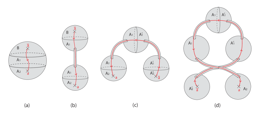
Figure 3: (a) Wave functional $|\Psi\rangle$. A Wilson line in representation $\hat{R}_{a}$ threads through the interface $A_{1}B$ and $A_{2}B$, respectively. (b) A three-manifold which is topologically equivalent to (a). (c) $\rho_{A_{1}\cup A_{2}}=\text{tr}_{B}|\Psi\rangle\langle\Psi|$, and (d) $\rho_{A_{1}\cup A_{2}}^{T_{A_{2}}}$, in which we do partial transposition over $A_{2}$, i.e., we switch $A_{2}$ with $A_{2}^{\prime}$ in (c).

First we consider the case where $A_{1}$ and $A_{2}$ are adjacent to each other, as shown in Fig. 3 (a). There is a Wilson line in representation $\hat{R}_{a}$ which threads through both the $A_{1}A_{2}$ interface and the $A_{1}B$ interface. Again, for the case without any quasiparticle on the sphere, one can simply set $\hat{R}_{a}=\hat{R}_{I}$ at the end.

For convenience, we deform the three-dimensional spacetime manifold in Fig. 3 (a), without changing the topology, to two three-balls connected by a tube, as shown in Fig. 3 (b). Then the reduced density matrix $\rho_{A_{1}\cup A_{2}}$ can be obtained by tracing over the $B$ part, as shown in Fig. 3 (c). Based on $\rho_{A_{1}\cup A_{2}}$, one can easily obtain $\rho_{A_{1}\cup A_{2}}^{T_{A_{2}}}$ by switching $A_{2}$ and $A_{2}^{\prime}$, as shown in Fig. 3 (d). One can find that the operation of partial transposition here is the same as that in Fig. 2.

Now we are ready to calculate $\text{tr}\left(\rho_{A_{1}\cup A_{2}}^{T_{A_{2}}}\right)^{n}$ as follows. We make $n$ copies of $\rho_{A_{1}\cup A_{2}}^{T_{A_{2}}}$, and glue the region $A_{1}^{\prime}$ ($A_{2}$) in the $i$-th copy with $A_{1}$ ($A_{2}^{\prime}$) in the $(i+1)$-th (mod $n$) copy. Similar with the case of a bipartitioned sphere, the result depends on whether $n$ is odd or even as follows.

For odd $n$, i.e., $n=n_{o}$, the resulting manifold is two $S^{3}$ connected by $n_{o}$ tubes. Each tube is contributed by the one that connects $A_{1}^{\prime}$ and $A_{1}^{\prime}$ in Fig. 3 (d). Then, by using the surgery procedure in Fig. 1, we cut all the tubes that connect the two $S^{3}$, with each tube contributing a factor $Z(S^{3},\hat{R}_{a})^{-1}$. Therefore, one can obtain

$$\begin{split}\frac{\text{tr}\left(\rho_{A_{1}\cup A_{2}}^{T_{A_{2}}}\right)^{n_{o}}}{\left(\text{tr}\rho_{A_{1}\cup A_{2}}^{T_{A_{2}}}\right)^{n_{o}}}=&\frac{1}{Z(S^{3},\hat{R}_{a})^{n_{o}}}\cdot\frac{Z(S^{3},\hat{R}_{a})^{2}}{Z(S^{3},\hat{R}_{a})^{n_{o}}}=Z(S^{3},\hat{R}_{a})^{2-2n_{o}}=\left(\mathcal{S}_{0a}\right)^{2-2n_{o}}.\end{split}$$ (2.30)

For even $n$, i.e., $n=n_{e}$, the resulting manifold is three $S^{3}$ connected by $n_{e}$ tubes. The extra $S^{3}$ has the same origin as the case of a bipartitiond sphere in Fig. 2. Similar with the $n=n_{o}$ case, by cutting each tube, one can obtain

$$\begin{split}\frac{\text{tr}\left(\rho_{A_{1}\cup A_{2}}^{T_{A_{2}}}\right)^{n_{e}}}{\left(\text{tr}\rho_{A_{1}\cup A_{2}}^{T_{A_{2}}}\right)^{n_{e}}}=&\frac{1}{Z(S^{3},\hat{R}_{a})^{n_{e}}}\cdot\frac{Z(S^{3},\hat{R}_{a})^{3}}{Z(S^{3},\hat{R}_{a})^{n_{e}}}=Z(S^{3},\hat{R}_{a})^{3-2n_{e}}=\left(\mathcal{S}_{0a}\right)^{3-2n_{e}}.\end{split}$$ (2.31)

Then the entanglement negativity between $A_{1}$ and $A_{2}$ can be expressed as

$$\mathcal{E}_{A_{1}A_{2}}=\lim_{n_{e}\to 1}\ln\frac{\text{tr}\left(\rho^{T_{B}}\right)^{n_{e}}}{\left(\text{tr}\rho^{T_{B}}\right)^{n_{e}}}=\ln\mathcal{S}_{0a}=\ln d_{a}-\ln\mathcal{D},$$ (2.32)

which is the same as Eq. (2.28). In other words, for a tripartitioned $S^{2}$ as shown in Fig. 3, the existence of region $B$ does not affect the entanglement negativity between $A_{1}$ and $A_{2}$, i.e.,

$$\mathcal{E}_{A_{1}A_{2}}(B\neq\emptyset)=\mathcal{E}_{A_{1}A_{2}}(B=\emptyset).$$ (2.33)

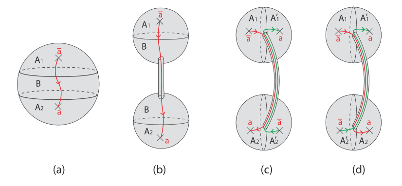
Figure 4: (a) Wave functional $|\Psi\rangle$. A Wilson line in representation $\hat{R}_{a}$ threads through the interface $A_{1}B$ and $A_{2}B$. $A_{1}$ and $A_{2}$ are disjoint. (b) A three-manifold which is topologically equivalent to (a). (c) $\rho_{A_{1}\cup A_{2}}=\text{tr}_{B}|\Psi\rangle\langle\Psi|$, and (d) $\rho_{A_{1}\cup A_{2}}^{T_{A_{2}}}$, in which we switch region $A_{2}$ and $A_{2}^{\prime}$ in (c).

2.2.2 Case of disjoint $A_{1}$ and $A_{2}$

Here, we consider the case that $A_{1}$ and $A_{2}$ are disjoint, as shown in Fig. 4 (a). We also include a quasiparticle $a$ (anti-quasiparticle $\bar{a}$) in region $A_{2}$ ($A_{1}$). Therefore, a Wilson line in representation $\hat{R}_{a}$ threads through both the $A_{1}B$ interface and the $A_{2}B$ interface.

The three-manifold in Fig. 4 (a) is equivalent to two three-balls connected by a tube, as shown in Fig. 4 (b). Based on this, one can obtain the reduced density matrix $\rho_{A_{1}\cup A_{2}}$, as shown in Fig.4 (c). To get the partially transposed reduced density matrix $\rho_{A_{1}\cup A_{2}}^{T_{A_{2}}}$, one simply needs to switch $A_{2}$ with $A_{2}^{\prime}$, as shown in Fig. 4 (d).

We now calculate the entanglement negativity between $A_{1}$ and $A_{2}$. As before, we make $n$ copies of $\rho_{A_{1}\cup A_{2}}^{T_{A_{2}}}$ in Fig. 4 (d). Then we glue region $A_{1}^{\prime}$ ($A_{2}$) in the $i$-th copy with the region $A_{1}$ ($A_{2}^{\prime}$) in the $(i+1)$-th (mod $n$) copy. In this way, we obtain $\text{tr}\left(\rho_{A_{1}\cup A_{2}}^{T_{A_{2}}}\right)^{n}$. It can be found that the resulting manifold is two $S^{3}$ connected by $n$ tubes, which is independent of whether $n$ is even or odd. By considering the surgery procedure in Fig. 1, one can cut all the tubes that connect the two $S^{3}$, with each tube contributing a factor $Z(S^{3},\hat{R}_{a})$. Then one can obtain

$$\begin{split}\frac{\text{tr}\left(\rho_{A_{1}\cup A_{2}}^{T_{A_{2}}}\right)^{n}}{\left(\text{tr}\rho_{A_{1}\cup A_{2}}^{T_{A_{2}}}\right)^{n}}=&\frac{1}{Z(S^{3},\hat{R}_{a})^{n}}\cdot\frac{Z(S^{3},\hat{R}_{a})^{2}}{Z(S^{3},\hat{R}_{a})^{n}}=Z(S^{3},\hat{R}_{a})^{2-2n}=\left(\mathcal{S}_{0a}\right)^{2-2n},\end{split}$$ (2.34)

for both $n=n_{o}$ and $n=n_{e}$. Therefore, one can obtain the entanglement negativity between $A_{1}$ and $A_{2}$ as follows

$$\mathcal{E}_{A_{1}A_{2}}=\lim_{n_{e}\to 1}\ln\frac{\text{tr}\left(\rho^{T_{B}}\right)^{n_{e}}}{\left(\text{tr}\rho^{T_{B}}\right)^{n_{e}}}=\ln\left(\mathcal{S}_{0a}\right)^{0}=0.$$ (2.35)

I.e., there is no entanglement negativity between $A_{1}$ and $A_{2}$ in this case. It is noted that the topological mutual information between $A_{1}$ and $A_{2}$ for this case is also zero [see Eq. (B.64)].

2.3 Two adjacent non-contractible regions on a torus with non-contractible $B$

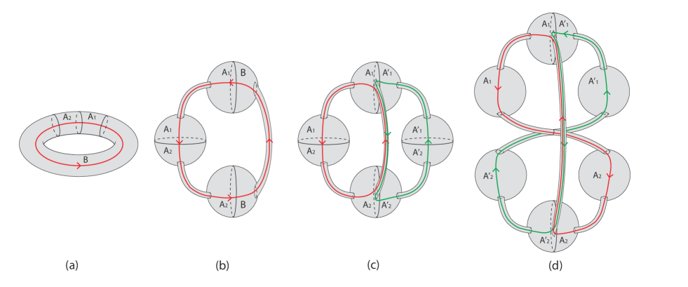
Figure 5: (a) Wave functional $|\Psi\rangle$. The toroidal space is divided into threes parts $A_{1}$, $A_{2}$ and $B$, where we have a one-component $A_{1}A_{2}$ interface. The red solid line represents a Wilson loop which can fluctuate among different representations. (b) A three-manifold with three $3$-balls joined by three tubes appropriately, which is topologically equivalent to (a). (c) $\rho_{A_{1}\cup A_{2}}=\text{tr}_{B}|\Psi\rangle\langle\Psi|$, and (d) $\rho_{A_{1}\cup A_{2}}^{T_{A_{2}}}$, in which we switch $A_{2}$ with $A_{2}^{\prime}$ in (c).

Here, we focus on the spatial manifold of a torus, $T^{2}$. For the simplest case of a bipartite torus, one can refer to the Appendix A, where the operation is straightforward and helpful for understanding the more complicated cases.

We first consider two adjacent non-contractible regions $A_{1}$ and $A_{2}$ on a torus with a non-contractible region $B$, but with different number of components for the interface, as shown in Fig. 5 (a) and Fig. 6 (a). In Fig. 5 (a), the two adjacent regions $A_{1}$ and $A_{2}$ share a one-component $A_{1}A_{2}$ interface, and in Fig. 6 (a), the two adjacent regions $A_{1}$ and $A_{2}$ share a two-component $A_{1}A_{2}$ interface. In the following, we will study the entanglement negativity between $A_{1}$ and $A_{2}$ for these two cases separately.

2.3.1 One-component interface

For the configuration in Fig. 5 (a), it is equivalent to three 3-balls connected by three tubes, as shown in Fig. 5 (b). Then one can obtain the reduced density matrix $\rho_{A_{1}\cup A_{2}}$ by tracing over the $B$ part, as shown in Fig. 5 (c). The partial transposition of the reduced density matrix $\rho_{A_{1}\cup A_{2}}$ is fulfilled by switching $A_{2}$ with $A_{2}^{\prime}$, as shown in Fig. 5 (d).

Generally, the Wilson loop can fluctuate among different representations. For simplicity, we first consider the case in which the Wilson loop is in a definite representation $\hat{R}_{a}$. To study $\text{tr}\left(\rho_{A_{1}\cup A_{2}}^{T_{A_{2}}}\right)^{n}$, we make $n$ copies of $\rho_{A_{1}\cup A_{2}}^{T_{A_{2}}}$ in Fig. 5 (d). Then we glue region $A_{1}^{\prime}$ ($A_{2}$) in the $i$-th copy with $A_{1}$ ($A_{2}^{\prime}$) in the $(i+1)$-th (mod $n$) copy, based on which we obtain $\text{tr}\left(\rho_{A_{1}\cup A_{2}}^{T_{A_{2}}}\right)^{n}$. The result after gluing depends on whether $n$ is odd or even as follows: For odd $n$, i.e., $n=n_{o}$, the resulting manifold is three $S^{3}$ connected by $3n_{o}$ tubes. The $3n_{o}$ tubes are contributed by the ones connecting $A_{1}^{\prime}-A_{1}^{\prime}$, $A_{1}-A_{1}$, $A_{2}-A_{2}$, $A_{2}^{\prime}-A_{2}^{\prime}$ and $B-B$, respectively. The tube connecting $B-B$ corresponds to the vertical tube in Fig. 5 (d). Then, by using the surgery procedure in Fig. 1, one can cut all the $3n_{o}$ tubes, with each tube contributing a factor $Z(S^{3},\hat{R}_{a})$. Then one can obtain

$$\begin{split}\frac{\text{tr}\left(\rho_{A_{1}\cup A_{2}}^{T_{A_{2}}}\right)^{n_{o}}}{\left(\text{tr}\rho_{A_{1}\cup A_{2}}^{T_{A_{2}}}\right)^{n_{o}}}=&\frac{1}{Z(S^{2}\times S^{1},\hat{R}_{a},\hat{\overline{R}}_{a})^{n_{o}}}\cdot\frac{Z(S^{3},\hat{R}_{a})^{3}}{Z(S^{3},\hat{R}_{a})^{3n_{o}}}=Z(S^{3},\hat{R}_{a})^{3-3n_{o}}=\left(\mathcal{S}_{0a}\right)^{3-3n_{o}},\end{split}$$ (2.36)

where we have used the fact $Z(S^{2}\times S^{1},\hat{R}_{a},\hat{\overline{R}}_{a})=1$. On the other hand, for even $n$, i.e., $n=n_{e}$, the resulting manifold is four $S^{3}$ connected by $3n_{e}$ tubes, where the extra $S^{3}$ is caused by the partial transposition. Similar with the case of $n=n_{o}$, the $3n_{e}$ tubes are contributed by the ones connecting $A_{1}^{\prime}-A_{1}^{\prime}$, $A_{1}-A_{1}$, $A_{2}-A_{2}$, $A_{2}^{\prime}-A_{2}^{\prime}$ and $B-B$, respectively. By cutting all the $3n_{e}$ tubes with surgery, one can immediately obtain

$$\begin{split}\frac{\text{tr}\left(\rho_{A_{1}\cup A_{2}}^{T_{A_{2}}}\right)^{n_{e}}}{\left(\text{tr}\rho_{A_{1}\cup A_{2}}^{T_{A_{2}}}\right)^{n_{e}}}=&\frac{1}{Z(S^{2}\times S^{1},\hat{R}_{a},\hat{\overline{R}}_{a})^{n_{e}}}\cdot\frac{Z(S^{3},\hat{R}_{a})^{4}}{Z(S^{3},\hat{R}_{a})^{3n_{e}}}=Z(S^{3},\hat{R}_{a})^{4-3n_{e}}=\left(\mathcal{S}_{0a}\right)^{4-3n_{e}}.\end{split}$$ (2.37)

It is then straightforward to show that for a general state $|\psi\rangle=\sum_{j}\psi_{j}|\hat{R}_{j}\rangle$, i.e., the Wilson loop is in a superposition of different representations $\hat{R}_{j}$, one has

$$\frac{\text{tr}\left(\rho_{A_{1}\cup A_{2}}^{T_{A_{2}}}\right)^{n_{o}}}{\left(\text{tr}\rho_{A_{1}\cup A_{2}}^{T_{A_{2}}}\right)^{n_{o}}}= \frac{\sum_{j}|\psi_{j}|^{2n_{o}}\left(\mathcal{S}_{0j}\right)^{3-3n_{o}}}{\left(\sum_{j}|\psi_{j}|^{2}\right)^{n_{o}}},$$

$$\frac{\text{tr}\left(\rho_{A_{1}\cup A_{2}}^{T_{A_{2}}}\right)^{n_{e}}}{\left(\text{tr}\rho_{A_{1}\cup A_{2}}^{T_{A_{2}}}\right)^{n_{e}}}= \frac{\sum_{j}|\psi_{j}|^{2n_{e}}\left(\mathcal{S}_{0j}\right)^{4-3n_{e}}}{\left(\sum_{j}|\psi_{j}|^{2}\right)^{n_{e}}}.$$ (2.38)

Then, one can obtain the entanglement negativity between $A_{1}$ and $A_{2}$ as follows

$$\mathcal{E}_{A_{1}A_{2}}=\lim_{n_{e}\to 1}\ln\text{tr}\frac{\text{tr}\left(\rho_{A_{1}\cup A_{2}}^{T_{A_{2}}}\right)^{n_{e}}}{\left(\text{tr}\rho_{A_{1}\cup A_{2}}^{T_{A_{2}}}\right)^{n_{e}}}=\ln\left(\sum_{j}|\psi_{j}|^{2}\mathcal{S}_{0j}\right)-\ln\sum_{j}|\psi_{j}|^{2}.$$ (2.39)

By imposing the normalization condition $\sum_{j}|\psi_{j}|^{2}=1$, $\mathcal{E}_{A_{1}A_{2}}$ can be simplified as

$$\mathcal{E}_{A_{1}A_{2}}=\ln\left(\sum_{j}|\psi_{j}|^{2}\mathcal{S}_{0j}\right)=\ln\left(\sum_{j}|\psi_{j}|^{2}d_{j}\right)-\ln\mathcal{D}.$$ (2.40)

Several comments on the above result are in orders:

1. By comparing with Eq. (A.58) for the case of a bipartitioned torus where $B=\emptyset$, it is found that $\mathcal{E}_{A_{1}A_{2}}(B\neq\emptyset)\neq\mathcal{E}_{A_{1}A_{2}}(B=\emptyset)$, which is different from the result for a tripartitioned sphere in Eq. (2.33). The reason is that for a torus geometry, as the region $B$ shrinks to $\emptyset$, the component of the $A_{1}A_{2}$ interface changes from one to two.

2. It is found that $\mathcal{E}_{A_{1}A_{2}}$ in Eq. (2.40) can be used to distinguish an Abelian theory from a non-Abelian theory. For an Abelian theory, we have $d_{j}=1$ for arbitrary representations $\hat{R}_{j}$, and therefore $\mathcal{E}_{A_{1}A_{2}}=-\ln\mathcal{D}$, which is independent of the choice of ground states. On the other hand, for a non-Abelian theory, there exists at least one representation $\hat{R}_{j}$ so that $d_{j}>1$. Therefore, for a non-Abelian theory, $\mathcal{E}_{A_{1}A_{2}}$ depends on the choice of ground states.

2.3.2 Two-component interface

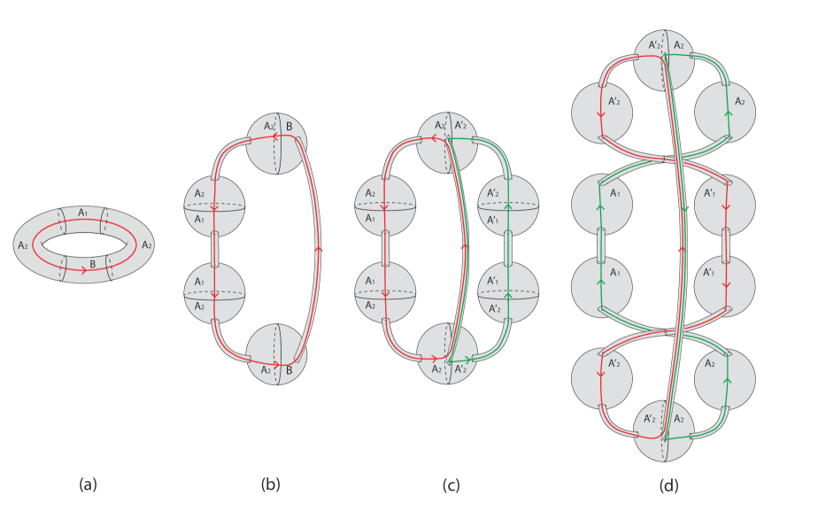
Figure 6: (a) Wave functional $|\Psi\rangle$. The toroidal space is divided into threes parts $A_{1}$, $A_{2}$ and $B$, where we have a two-component $A_{1}A_{2}$ interface. The red solid line represents a Wilson loop which can fluctuate among different representations. (b ) A three-manifold with four $3$-balls joined by four tubes appropriately, which is equivalent to the configuration in (a) in topology. (c) $\rho_{A_{1}\cup A_{2}}=\text{tr}_{B}|\Psi\rangle\langle\Psi|$, and (d) $\rho_{A_{1}\cup A_{2}}^{T_{A_{2}}}$, in which we do partial transposition over $A_{2}$, i.e., we switch $A_{2}$ with $A_{2}^{\prime}$ in (c).

Next, we consider two adjacent non-contractible regions $A_{1}$ and $A_{2}$ on a spatial manifold $T^{2}$, with a two-component $A_{1}A_{2}$ interface, as shown in Fig. 6 (a). The configuration in Fig. 6 (a) is equivalent to four 3-balls connected by four tubes in topology, as shown in Fig. 6 (b). Then it is straightforward to obtain the reduced density matrix $\rho_{A_{1}\cup A_{2}}$ by tracing out the $B$ part, as shown in Fig. 6 (c). Next, for the partially transposed reduced density matrix $\rho^{T_{A_{2}}}_{A_{1}\cup A_{2}}$, we simply need to switch $A_{2}$ with $A_{2}^{\prime}$, as shown in Fig. 6 (d).

As in the previous part, we first consider the simple case that the Wilson loop is in a definite representation $\hat{R}_{a}$. To calculate $\text{tr}\left(\rho_{A_{1}\cup A_{2}}^{T_{A_{2}}}\right)^{n}$, we make $n$ copies of $\rho_{A_{1}\cup A_{2}}^{T_{2}}$ in Fig. 6 (d). Then by gluing the region $A_{1}^{\prime}$($A_{2}$) in the $i$-th copy with the region $A_{1}$($A_{2}^{\prime}$) in the $(i+1)$-th (mod $n$) copy, we can obtain $\text{tr}\left(\rho_{A_{1}\cup A_{2}}^{T_{A_{2}}}\right)^{n}$. As before, the resulting manifold depends on whether $n$ is odd or even, as follows. For odd $n$, i.e., $n=n_{o}$, the resulting manifold is four $S^{3}$ connected by $4n_{o}$ tubes. The $4n_{o}$ tubes are contributed by the ones connecting $A_{2}-A_{2}$, $A_{1}^{\prime}-A_{1}^{\prime}$, $A_{1}-A_{1}$, $A_{2}^{\prime}-A_{2}^{\prime}$ and $B-B$, respectively. By using the surgery procedure in Fig. 1, we can cut all the $4n_{o}$ tubes, with each tube contributing $Z(S^{3},\hat{R}_{a})$. Therefore, one can obtain

$$\begin{split}\frac{\text{tr}\left(\rho_{A_{1}\cup A_{2}}^{T_{A_{2}}}\right)^{n_{o}}}{\left(\text{tr}\rho_{A_{1}\cup A_{2}}^{T_{A_{2}}}\right)^{n_{o}}}=&\frac{1}{Z(S^{2}\times S^{1},\hat{R}_{a},\hat{\overline{R}}_{a})^{n_{o}}}\cdot\frac{Z(S^{3},\hat{R}_{a})^{4}}{Z(S^{3},\hat{R}_{a})^{4n_{o}}}=Z(S^{3},\hat{R}_{a})^{4-4n_{o}}=\left(\mathcal{S}_{0a}\right)^{4-4n_{o}}.\end{split}$$ (2.41)

On the other hand, for even $n$, i.e., $n=n_{e}$, the resulting manifold is six $S^{3}$ connected by $3n_{e}$ tubes, where the extra two $S^{3}$ is caused by the partial transposition. Similar with the case of $n=n_{o}$, the $4n_{e}$ tubes are contributed by the ones connecting $A_{2}-A_{2}$, $A_{1}^{\prime}-A_{1}^{\prime}$, $A_{1}-A_{1}$, $A_{2}^{\prime}-A_{2}^{\prime}$ and $B-B$, respectively. With the surgery method, one can immediately obtain

$$\begin{split}\frac{\text{tr}\left(\rho_{A_{1}\cup A_{2}}^{T_{A_{2}}}\right)^{n_{e}}}{\left(\text{tr}\rho_{A_{1}\cup A_{2}}^{T_{A_{2}}}\right)^{n_{e}}}=&\frac{1}{Z(S^{2}\times S^{1},\hat{R}_{a},\hat{\overline{R}}_{a})^{n_{e}}}\cdot\frac{Z(S^{3},\hat{R}_{a})^{6}}{Z(S^{3},\hat{R}_{a})^{4n_{e}}}=Z(S^{3},\hat{R}_{a})^{6-4n_{e}}=\left(\mathcal{S}_{0a}\right)^{6-4n_{e}}.\end{split}$$ (2.42)

It is then straightforward to show that for a general state $|\psi\rangle=\sum_{j}\psi_{j}|\hat{R}_{j}\rangle$, one has

$$\frac{\text{tr}\left(\rho_{A_{1}\cup A_{2}}^{T_{A_{2}}}\right)^{n_{o}}}{\left(\text{tr}\rho_{A_{1}\cup A_{2}}^{T_{A_{2}}}\right)^{n_{o}}} =\frac{\sum_{j}|\psi_{j}|^{2n_{o}}\left(\mathcal{S}_{0j}\right)^{4-4n_{o}}}{\left(\sum_{j}|\psi_{j}|^{2}\right)^{n_{o}}},$$

$$\frac{\text{tr}\left(\rho_{A_{1}\cup A_{2}}^{T_{A_{2}}}\right)^{n_{e}}}{\left(\text{tr}\rho_{A_{1}\cup A_{2}}^{T_{A_{2}}}\right)^{n_{e}}} =\frac{\sum_{j}|\psi_{j}|^{2n_{e}}\left(\mathcal{S}_{0j}\right)^{6-4n_{e}}}{\left(\sum_{j}|\psi_{j}|^{2}\right)^{n_{e}}}.$$ (2.43)

Then, one can obtain the entanglement negativity between $A_{1}$ and $A_{2}$ as follows

$$\mathcal{E}_{A_{1}A_{2}}=\lim_{n_{e}\to 1}\ln\text{tr}\frac{\text{tr}\left(\rho_{A_{1}\cup A_{2}}^{T_{A_{2}}}\right)^{n_{e}}}{\left(\text{tr}\rho_{A_{1}\cup A_{2}}^{T_{A_{2}}}\right)^{n_{e}}}=\ln\left(\sum_{j}|\psi_{j}|^{2}\mathcal{S}_{0j}^{2}\right)-\ln\sum_{j}|\psi_{j}|^{2}.$$ (2.44)

By imposing the normalization condition $\sum_{j}|\psi_{j}|^{2}=1$, $\mathcal{E}_{A_{1}A_{2}}$ can be simplified as

$$\mathcal{E}_{A_{1}A_{2}}=\ln\left(\sum_{j}|\psi_{j}|^{2}\mathcal{S}_{0j}^{2}\right)=\ln\left(\sum_{j}|\psi_{j}|^{2}d_{j}^{2}\right)-2\ln\mathcal{D}.$$ (2.45)

Compared with the case of one-component $A_{1}A_{2}$ interface in the previous part [see Eq. (2.40)], here the power of $\mathcal{S}_{0j}$ is changed from $1$ to $2$, which is caused by changing the number of components in $A_{1}A_{2}$ interface. In addition, similar with the result in Eq. (2.40), $\mathcal{E}_{A_{1}A_{2}}$ in Eq. (2.45) can also be used to distinguish an Abelian theory from a non-Abelian theory by studying its dependence on the choice of ground states.

2.4 Two adjacent non-contractible regions on a torus with contractible $B$

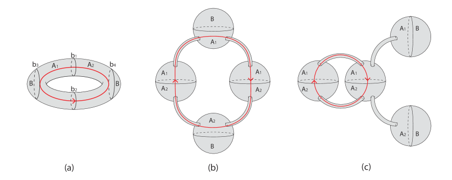
Figure 7: (a) Wave functional $|\Psi\rangle$. The toroidal space is divided into threes parts $A_{1}$, $A_{2}$ and $B$, where we have a two-component $A_{1}A_{2}$ interface and a contractible region $B$. The red solid line represents a Wilson loop which can fluctuate among different representations. (b) A three-manifold with four $3$-balls joined by four tubes appropriately, which is equivalent to the configuration in (a) in topology. The configuration in (b) can be further deformed into the configuration in (c), without changing topology.

Here, we study the entanglement negativity between two adjacent non-contractible regions $A_{1}$ and $A_{2}$ on a spatial manifold $T^{2}$, with a contractible region $B$, as shown in Fig. 7 (a). For convenience, we deform the three-manifold in Fig. 7 (a) into the three-manifold in Fig. 7 (b), where there are four $S^{3}$ connected by four tubes, which can be further deformed into the three-manifold in Fig. 7 (c). Then it is straightforward to obtain the reduced density matrix $\rho_{A_{1}A_{2}}$ by tracing out the $B$ part, as shown in Fig. 8 (a). To obtain the partially transposed reduced density matrix $\rho_{A_{1}\cup A_{2}}^{T_{A_{2}}}$, we simply need to switch $A_{2}$ with $A_{2}^{\prime}$ in $\rho_{A_{1}\cup A_{2}}$, as shown in Fig. 8 (b).

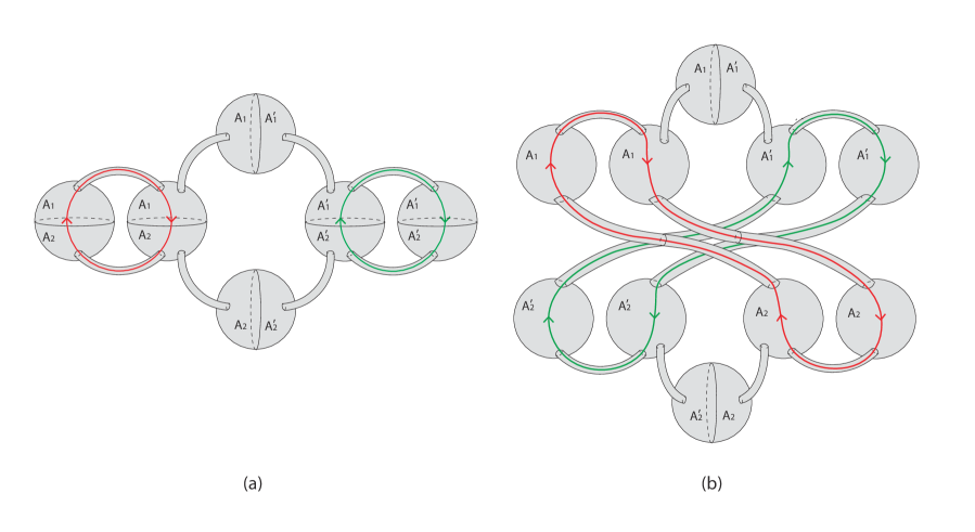
Figure 8: (a) The reduced density matrix $\rho_{A_{1}\cup A_{2}}$, which is obtained based on the wave functional in Fig.7 (c). (b) The partially transposed reduced density matrix $\rho_{A_{1}\cup A_{2}}^{T_{A_{2}}}$, which is obtained by switching $A_{2}$ and $A_{2}^{\prime}$ in (a).

As before, for simplicity, we first consider the case in which the Wilson loop is in a definite representation $\hat{R}_{a}$. To obtain $\text{tr}\left(\rho_{A_{1}\cup A_{2}}^{T_{A_{2}}}\right)^{n}$, we make $n$ copies of $\rho_{A_{1}\cup A_{2}}^{T_{A_{2}}}$ in Fig. 8 (b). Then we glue the region $A_{1}^{\prime}$($A_{2}$) in the $i$-th copy with the region $A_{1}$($A_{2}^{\prime}$) in the $(i+1)$-th (mod $n$) copy, and obtain $\text{tr}\left(\rho_{A_{1}\cup A_{2}}^{T_{A_{2}}}\right)^{n}$. Since the configuration in Fig. 8 (b) is already very complicated, it is helpful for the readers to understand the gluing based on the case of a bipartite torus [see Fig. 10 (c)], considering that the limit $B\to\emptyset$ in Fig. 7 (a) corresponds to a bipartitioned torus.

The gluing result depends on whether $n$ is odd or even as follows. For odd $n$, i.e., $n=n_{o}$, the resulting manifold is four $S^{3}$ connected by $4n_{o}$ tubes. One should be very careful here. For convenience, we label the four rows of 3-balls in Fig. 8 (d) as the first, second, third and fourth rows of 3-balls from top to bottom. In the resulting manifold after gluing, two $S^{3}$ are contributed by the 3-balls in the first and fourth rows in Fig. 8 (d). It is noted that there is no Wilson line threading through these two $S^{3}$, and therefore each of them contributes $Z(S^{3})$ after the surgery. The other two $S^{3}$ are contributed by the 3-balls in the second and third rows. Since there are Wilson lines threading through these two $S^{3}$, each of them contributes $Z(S^{3},\hat{R}_{a})$ after the surgery.

For the $4n_{o}$ tubes, $2n_{o}$ tubes are contributed by the ones that connect the first (third) and second (fourth) rows of 3-balls. There are no Wilson lines threading through these $2n_{o}$ tubes. Therefore, after the surgery procedure in Fig. 1, each of these tubes contributes $Z(S^{3})$. The other $2n_{o}$ tubes are contributed by the tubes that connect $A_{1}-A_{1}$ ($A_{1}^{\prime}-A_{1}^{\prime}$) in the second row, and the ones that connect $A_{2}^{\prime}-A_{2}^{\prime}$ ($A_{2}-A_{2}$) in the third row. For these $2n_{o}$ tubes, since there are Wilson lines threading through them, each tube contributes a factor $Z(S^{3},\hat{R}_{a})$ after the surgery.

Based on the above analysis, one can obtain

$$\frac{\text{tr}\left(\rho_{A_{1}\cup A_{2}}^{T_{A_{2}}}\right)^{n_{o}}}{\left(\text{tr}\rho_{A_{1}\cup A_{2}}^{T_{A_{2}}}\right)^{n_{o}}} =\frac{1}{Z(S^{2}\times S^{1};\hat{R}_{a},\hat{\overline{R}}_{a})^{n_{o}}}\cdot\frac{Z(S^{3})^{2}\cdot Z(S^{3},\hat{R}_{a})^{2}}{Z(S^{3})^{2n_{o}}\cdot Z(S^{3},\hat{R}_{a})^{2n_{o}}}$$

$$=Z(S^{3})^{2-2n_{o}}\cdot Z(S^{3},\hat{R}_{a})^{2-2n_{o}}$$

$$=\left(\mathcal{S}_{00}\right)^{2-2n_{o}}\left(\mathcal{S}_{0a}\right)^{2-2n_{o}}.$$ (2.46)

On the other hand, for even $n$, i.e., $n=n_{e}$, the resulting manifold is six $S^{3}$ connected by $4n_{e}$ tubes. Compared with the case of $n=n_{o}$, the extra two $S^{3}$ are introduced by the partial transposition, which is similar to the case of a bipartite torus in Fig. 10. In particular, for the extra two $S^{3}$, there are Wilson lines threading through them, and therefore each of them contributes $Z(S^{3},\hat{R}_{a})$ after the surgery. Therefore, one can obtain

$$\frac{\text{tr}\left(\rho_{A_{1}\cup A_{2}}^{T_{A_{2}}}\right)^{n_{e}}}{\left(\text{tr}\rho_{A_{1}\cup A_{2}}^{T_{A_{2}}}\right)^{n_{e}}} =\frac{1}{Z(S^{2}\times S^{1};\hat{R}_{a},\hat{\overline{R}}_{a})^{n_{e}}}\cdot\frac{Z(S^{3})^{2}}{Z(S^{3})^{2n_{e}}}\cdot\left[\frac{Z(S^{3},\hat{R}_{a})^{2}}{Z(S^{3},\hat{R}_{a})^{n_{e}}}\right]^{2}$$

$$=Z(S^{3})^{2-2n_{e}}\cdot Z(S^{3},\hat{R}_{a})^{4-2n_{e}}$$

$$=\left(\mathcal{S}_{00}\right)^{2-2n_{e}}\left(\mathcal{S}_{0j}\right)^{4-2n_{e}}.$$ (2.47)

It is emphasized that the square term $[\cdots]^{2}$ in the first row arises from the fact that the two sets of Wilson loops (red and green) in Fig. 8 (b), after gluing $2n_{e}$ copies, are independent to each other. This square term is absent in Eq. (2.4), because the two sets of Wilson loops are glued to each other for $n=n_{o}$.

It is straightforward to check that for a general state $|\psi\rangle=\sum_{i}\psi_{i}|\hat{R}_{i}\rangle$, one has

$$\frac{\text{tr}\left(\rho_{A_{1}\cup A_{2}}^{T_{A_{2}}}\right)^{n_{o}}}{\left(\text{tr}\rho_{A_{1}\cup A_{2}}^{T_{A_{2}}}\right)^{n_{o}}} =\left(\mathcal{S}_{00}\right)^{2-2n_{0}}\cdot\frac{\sum_{j}|\psi_{j}|^{2n_{o}}\left(\mathcal{S}_{0j}\right)^{2-2n_{o}}}{\left(\sum_{j}|\psi_{j}|^{2}\right)^{n_{o}}},$$

$$\frac{\text{tr}\left(\rho_{A_{1}\cup A_{2}}^{T_{A_{2}}}\right)^{n_{e}}}{\left(\text{tr}\rho_{A_{1}\cup A_{2}}^{T_{A_{2}}}\right)^{n_{e}}} =\left(\mathcal{S}_{00}\right)^{2-2n_{e}}\cdot\frac{\left[\sum_{j}|\psi_{j}|^{n_{e}}\left(\mathcal{S}_{0j}\right)^{2-n_{e}}\right]^{2}}{\left(\sum_{j}|\psi_{j}|^{2}\right)^{n_{e}}}.$$ (2.48)

Then, one can obtain the entanglement negativity between $A_{1}$ and $A_{2}$ as follows

$$\mathcal{E}_{A_{1}A_{2}}=\lim_{n_{e}\to 1}\ln\text{tr}\frac{\text{tr}\left(\rho_{A_{1}\cup A_{2}}^{T_{A_{2}}}\right)^{n_{e}}}{\left(\text{tr}\rho_{A_{1}\cup A_{2}}^{T_{A_{2}}}\right)^{n_{e}}}=2\ln\left(\sum_{j}|\psi_{j}|\mathcal{S}_{0j}\right)-\ln\sum_{j}|\psi_{j}|^{2}.$$ (2.49)

By imposing the normalization condition $\sum_{j}|\psi_{j}|^{2}=1$, $\mathcal{E}_{A_{1}A_{2}}$ can be simplified as

$$\mathcal{E}_{A_{1}A_{2}}=2\ln\left(\sum_{j}|\psi_{j}|\mathcal{S}_{0j}\right)=2\ln\left(\sum_{j}|\psi_{j}|d_{j}\right)-2\ln\mathcal{D}.$$ (2.50)

The result is the same as Eq. (A.58) for a bipartite torus, i.e., $\mathcal{E}_{A_{1}A_{2}}(B\neq\emptyset)=\mathcal{E}_{A_{1}A_{2}}(B=\emptyset)$ for the configuration in Fig. 7 (a). For this case, the entanglement negativity between $A_{1}$ and $A_{2}$ depends on the choice of ground states for both Abelian and non-Abelian Chern-Simons theories.

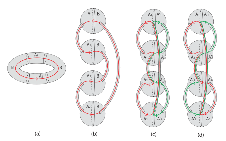
Figure 9: (a) Wave functional $|\Psi\rangle$. The toroidal space is divided into threes parts $A_{1}$, $A_{2}$ and $B$, where $A_{1}$ and $A_{2}$ are disjoint. (b) The configuration in (a) is topologically equivalent to four $3$-balls joined by four tubes appropriately. (c) $\rho_{A_{1}\cup A_{2}}$ by tracing out part $B$. (d) Partially transposed reduced density matrix $\rho_{A_{1}\cup A_{2}}^{T_{2}}$ where the partial transposition is over degrees of freedom in $A_{2}$, i.e., we switch $A_{2}$ with $A_{2}^{\prime}$ in $\rho_{A_{1}\cup A_{2}}$ in (c).

2.5 Two disjoint non-contractible regions on a torus

Finally, we demonstrate the vanishing entanglement negativity for two disjoint non-contractible regions $A_{1}$ and $A_{2}$ on a spatial manifold $T^{2}$, as shown in Fig. 9 (a), in which the regions $A_{1}$ and $A_{2}$ are separated by non-contractible regions $B$. The configuration in Fig. 9 (a) is topologically equivalent to four $3$-balls connected by four tubes appropriately, as shown in Fig. 9 (b). Then it is straightforward to obtain the reduced density matrix $\rho_{A_{1}\cup A_{2}}$ by tracing out the $B$ part, as shown in Fig. 9 (c). The partially transposed reduced density matrix $\rho_{A_{1}\cup A_{2}}^{T_{A_{2}}}$ in Fig. 9 (d) is obtained by switching $A_{2}$ and $A_{2}^{\prime}$ in Fig. 9 (c).

As before, we first consider the simple case that the Wilson loop is in a definite representation $\hat{R}_{a}$. By repeating the gluing and surgery procedures as before, it is straightforward to check that

$$\frac{\text{tr}\left(\rho_{A_{1}\cup A_{2}}^{T_{A_{2}}}\right)^{n_{o}}}{\left(\text{tr}\rho_{A_{1}\cup A_{2}}^{T_{A_{2}}}\right)^{n_{o}}} =\frac{1}{Z(S^{2}\times S^{1};\hat{R}_{a},\hat{\overline{R}}_{a})^{n_{o}}}\cdot\frac{Z(S^{3},\hat{R}_{a})^{4}}{Z(S^{3},\hat{R}_{a})^{4n_{o}}}=Z(S^{3},\hat{R}_{a})^{4-4n_{o}}=\left(\mathcal{S}_{0a}\right)^{4(1-n_{o})},$$

$$\frac{\text{tr}\left(\rho_{A_{1}\cup A_{2}}^{T_{A_{2}}}\right)^{n_{e}}}{\left(\text{tr}\rho_{A_{1}\cup A_{2}}^{T_{A_{2}}}\right)^{n_{e}}} =\frac{1}{Z(S^{2}\times S^{1};\hat{R}_{a},\hat{\overline{R}}_{a})^{n_{e}}}\cdot\frac{Z(S^{3},\hat{R}_{a})^{4}}{Z(S^{3},\hat{R}_{a})^{4n_{e}}}=Z(S^{3},\hat{R}_{a})^{4-4n_{e}}=\left(\mathcal{S}_{0a}\right)^{4(1-n_{e})}.$$ (2.51)

The result is independent of whether $n$ is odd or even. For a general state $|\psi\rangle=\sum_{i}\psi_{i}|\hat{R}_{i}\rangle$, one can find that

$$\begin{split}\frac{\text{tr}\left(\rho_{A_{1}\cup A_{2}}^{T_{A_{2}}}\right)^{n_{o}(n_{e})}}{\left(\text{tr}\rho_{A_{1}\cup A_{2}}^{T_{A_{2}}}\right)^{n_{o}(n_{e})}}=\frac{\sum_{i}|\psi_{i}|^{2n_{o}(n_{e})}\left(\mathcal{S}_{0i}\right)^{4(1-n_{o}(n_{e}))}}{\left(\sum_{i}|\psi_{i}|^{2}\right)^{n_{o}(n_{e})}}.\end{split}$$ (2.52)

Then, one can obtain the entanglement negativity between $A_{1}$ and $A_{2}$ as follows

$$\mathcal{E}_{A_{1}A_{2}}=\lim_{n_{e}\to 1}\ln\frac{\text{tr}\left(\rho_{A_{1}\cup A_{2}}^{T_{A_{2}}}\right)^{n_{e}}}{\left(\text{tr}\rho_{A_{1}\cup A_{2}}^{T_{A_{2}}}\right)^{n_{e}}}=0,$$ (2.53)

i.e., there is no entanglement negativity between two disjoint non-contractible regions on a torus.

3 Concluding remarks

In this work, by using the surgery method and the replica trick, we compute the topological entanglement negativity between two spatial regions for Chern-Simons field theories. We study examples on various manifolds with different bipartitions or tripartitions. In particular, we study how the entanglement negativity depends on the distributions of quasiparticles and the choice of ground states. For two adjacent non-contractible regions on a tripartitioned torus, the entanglement negativity is dependent (independent) on the choice of ground states for non-Ablelian (Abelian) theories. Therefore, it provides a simple way to distinguish Abelian and non-Abelian theories. Our method applies to arbitrary oriented (2+1) dimensional manifolds with arbitrary ways of bipartions/tripartitions.

All the cases studied in this work agree with the results obtained by using a complimentary approach, the edge theory approach, presented in Ref. [26]. Here we would like to give some remarks on comparing the method in this work and the edge theory approach: (1) For the edge theory approach, it is unnecessary to know the (2+1) dimensional spacetime manifold and gluing pictures, which are usually complicated. By expressing the (Ishibashi) edge states at the entanglement cut, a straightforward calculation can be performed, which is usually tedious. (2) On the other hand, for the surgery approach shown in this work, the only complication is understanding the 3-manifold. However, this method is elegant, in the sense that once the corresponding 3-manifold for the partially transposed reduced density matrix is known, the results can be directly read off. Thus, these two methods are complimentary and have their own merits.

Finally, we close by pointing out a future problem: It is interesting to generalize our method(s) to higher dimensions, such as (3+1) dimensions. Most recently, the surgery of (3+1)-dimensional manifolds (with particle and loop excitations) was discussed in Ref. [41, 42]. One can study the entanglement entropy and negativity of (3+1)-dimensional TQFTs, once the corresponding partition function can be evaluated.

Appendix A Topological entanglement negativity: Bipartitioned torus

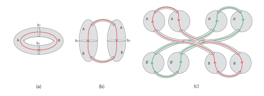
Figure 10: (a) Wave functional $|\Psi\rangle$. The toroidal space is bipartitioned into $A$ and $B$. (b) The configuration in (a) can be deformed to two $3$-balls joined by two tubes appropriately. (c) Partially transposed reduced density matrix $\rho_{A\cup B}^{T_{B}}$, where the partial transposition is fulfilled by switching $B$ and $B^{\prime}$.

Here, we consider a bipartitioned torus, as shown in Fig. 10 (a), which is topologically equivalent to two 3-balls connected by two tubes as shown in Fig. 10 (b). It is straightforward to obtain the partially transposed reduced density matrix $\rho_{AB}^{T_{B}}$ as shown in Fig. 10 (c).

For the first step, we consider the simplest case, i.e., the Wilson loop is in a definite representation $\hat{R}_{a}$. We follow the replica trick introduced in the main text: First, we make $n$ copies of $\rho_{AB}^{T_{B}}$ as in Fig. 9 (c). Then, we glue the region $A^{\prime}$($B$) in the $i$-th copy with the region $A$($B^{\prime}$) in the $(i+1)$-th (mod $n$) copy, based on which we obtain $\text{tr}\left(\rho_{AB}^{T_{B}}\right)^{n}$. One can find that the resulting manifold depends on whether $n$ is odd or even. For odd $n$, i.e., $n=n_{o}$, we obtain two $S^{3}$ connected by $2n_{o}$ tubes. It should be noted that these tubes are contributed by those connecting $A-A$, $A^{\prime}-A^{\prime}$, $B-B$, and $B^{\prime}-B^{\prime}$ in Fig. 10 (c). By considering the surgery procedure in Fig. 1, we cut all the $2n_{o}$ tubes, with each tube contributing $Z(S^{3},\hat{R}_{a})$. Then we can obtain

$$\frac{\text{tr}\left(\rho_{A\cup B}^{T_{B}}\right)^{n_{o}}}{\left(\text{tr}\rho_{A\cup B}^{T_{B}}\right)^{n_{o}}}= \frac{1}{Z(S^{2}\times S^{1},\hat{R}_{a},\hat{\overline{R}}_{a})^{n_{o}}}\cdot\frac{Z(S^{3},\hat{R}_{a})^{2}}{Z(S^{3},\hat{R}_{a})^{2n_{o}}}=Z(S^{3},\hat{R}_{a})^{2-2n_{o}}=\left(\mathcal{S}_{0a}\right)^{2-2n_{o}},$$ (A.54)

where we have used the fact that $\text{tr}\rho_{A\cup B}^{T_{B}}=Z(S^{2}\times S^{1},\hat{R}_{a},\hat{\overline{R}}_{a})=1$. On the other hand, for even $n$, i.e., $n=n_{e}$, the resulting manifold is composed of two independent manifolds, with each manifold being two $S^{3}$ connected by $n_{e}$ tubes. By using the same surgery procedure as above, we can obtain

$$\frac{\text{tr}\left(\rho_{A\cup B}^{T_{B}}\right)^{n_{e}}}{\left(\text{tr}\rho_{A\cup B}^{T_{B}}\right)^{n_{e}}}= \frac{1}{Z(S^{2}\times S^{1},\hat{R}_{a},\hat{\overline{R}}_{a})^{n_{e}}}\cdot\left[\frac{Z(S^{3},\hat{R}_{a})^{2}}{Z(S^{3},\hat{R}_{a})^{n_{e}}}\right]^{2}=Z(S^{3},\hat{R}_{a})^{4-2n_{e}}=\left(\mathcal{S}_{0a}\right)^{4-2n_{e}}.$$ (A.55)

It is then straightforward to show that for a general pure state $|\psi\rangle=\sum_{j}\psi_{j}|\hat{R}_{j}\rangle$, i.e., the Wilson loop is in a superposition of different representations, one has

$$\frac{\text{tr}\left(\rho_{A\cup B}^{T_{B}}\right)^{n_{o}}}{\left(\text{tr}\rho_{A\cup B}^{T_{B}}\right)^{n_{o}}}= \frac{\sum_{j}|\psi_{j}|^{2n_{o}}\left(\mathcal{S}_{0j}\right)^{2-2n_{o}}}{\left(\sum_{j}|\psi_{j}|^{2}\right)^{n_{o}}},$$

$$\frac{\text{tr}\left(\rho_{A\cup B}^{T_{B}}\right)^{n_{e}}}{\left(\text{tr}\rho_{A\cup B}^{T_{B}}\right)^{n_{e}}}= \frac{\left[\sum_{j}|\psi_{j}|^{n_{e}}\left(\mathcal{S}_{0j}\right)^{2-n_{e}}\right]^{2}}{\left(\sum_{j}|\psi_{j}|^{2}\right)^{n_{e}}}.$$ (A.56)

Then one can obtain the entanglement negativity between $A$ and $B$ as follows

$$\mathcal{E}_{AB}=\lim_{n_{e}\to 1}\ln\text{tr}\frac{\text{tr}\left(\rho_{A\cup B}^{T_{B}}\right)^{n_{e}}}{\left(\text{tr}\rho_{A\cup B}^{T_{B}}\right)^{n_{e}}}=2\ln\left(\sum_{j}|\psi_{j}|\mathcal{S}_{0j}\right)-\ln\sum_{j}|\psi_{j}|^{2}.$$ (A.57)

By imposing the normalization condition $\sum_{j}|\psi_{j}|^{2}=1$, $\mathcal{E}_{AB}$ can be simplified as

$$\mathcal{E}_{AB}=2\ln\left(\sum_{j}|\psi_{j}|\mathcal{S}_{0j}\right)=2\ln\left(\sum_{j}|\psi_{j}|d_{j}\right)-2\ln\mathcal{D},$$ (A.58)

which is the same as the $\frac{1}{2}$-Renyi entropy $S_{A}^{(1/2)}$ ($S_{B}^{(1/2)}$), as expected.

Appendix B Topological mutual information between two regions for various cases

Here, we make a comparison between the mutual information and the entanglement negativity between two regions $A_{1}$ and $A_{2}$ for various cases. It is noted that the mutual information in Chern-Simons theories is also studied for some specific cases in a recent paper [43].

B.1 Tripartitioned sphere

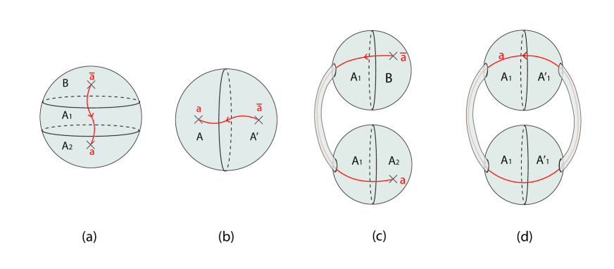
Figure 11: (a) Wave functional $|\Psi\rangle$. A Wilson line in representation $\hat{R}_{a}$ threads through the interface $A_{1}B$ and $A_{2}B$, respectively. (b) $\rho_{A}=\text{tr}_{B}|\Psi\rangle\langle\Psi|$. (c) Wave functional $|\Psi\rangle$, which is topologically equivalent to (a). (d) $\rho_{A_{1}}=\text{tr}_{A_{2}\cup B}|\Psi\rangle\langle\Psi|$.

B.1.1 Case of adjacent $A_{1}$ and $A_{2}$

This case corresponds to the configuration in Fig. 3 (a) [see also Fig. 11 (a)]. First, we calculate the entanglement entropy for $A=A_{1}\cup A_{2}$. Based on the configuration of $\rho_{A}$ in Fig. 11 (b), it is straightforward to check that

$$\text{tr}\left(\rho_{A}^{n}\right)=Z(S^{3},\hat{R}_{a})\quad\text{and}\quad\text{tr}\rho_{A}=Z(S^{3},\hat{R}_{a}).$$ (B.59)

Therefore,

$$S_{A}^{(n)}=\frac{1}{1-n}\ln\frac{\text{tr}\left(\rho_{A}^{n}\right)}{\left(\text{tr}\rho_{A}\right)^{n}}=\ln Z(S^{3},R_{a})=\ln\mathcal{S}_{0a}.$$ (B.60)

Observing the topology in Fig. 11 (a), it is straightforward to check that $S_{A_{2}}^{(n)}=S_{A}^{(n)}$. Next, to calculate the entanglement entropy for $A_{1}$, we deform the configuration of $|\Psi\rangle$ into Fig. 11 (c), based on which one can obtain $\rho_{A_{1}}$ in Fig. 11 (d). Then, one has

$$\text{tr}\left(\rho_{A_{1}}^{n}\right)=\frac{Z(S^{3},\hat{R}_{a})\cdot Z(S^{3},\hat{R}_{a})}{\left[Z(S^{3},\hat{R}_{a})\right]^{n}},$$ (B.61)

and

$$\begin{split}S_{A_{1}}^{(n)}=&\frac{1}{1-n}\ln\frac{\text{tr}\left(\rho_{A_{1}}^{n}\right)}{\left(\text{tr}\rho_{A_{1}}\right)^{n}}\\ =&\frac{1}{1-n}\ln\frac{Z(S^{3},\hat{R}_{a})\cdot Z(S^{3},\hat{R}_{a})}{\left[Z(S^{3},\hat{R}_{a})\right]^{2n}}\\ =&2\ln\mathcal{S}_{0a}.\end{split}$$ (B.62)

Therefore, the mutual information between $A_{1}$ and $A_{2}$ is given by

$$I^{(n)}_{A_{1},A_{2}}=S_{A_{1}}^{(n)}+S_{A_{2}}^{(n)}-S_{A_{1}\cup A_{2}}^{(n)}=2\ln\mathcal{S}_{0a}=2\ln d_{a}-2\ln\mathcal{D},$$ (B.63)

which is independent of $n$.

B.1.2 Case of disjoint $A_{1}$ and $A_{2}$

This case corresponds to the configuration in Fig. 4, and can be easily studied based on the previous results. It can be found that $S_{A_{1}}^{(n)}$ and $S_{A_{2}}^{(n)}$ have the same form as $S_{A}^{(n)}$ in Eq. (B.60). In addition, since the total system stays in a pure state, then we have $S_{A_{1}\cup A_{2}}^{(n)}=S_{B}^{(n)}$, which has the same expression as Eq. (B.62). Then one has

$$I^{(n)}_{A_{1},A_{2}}=S_{A_{1}}^{(n)}+S_{A_{2}}^{(n)}-S_{A_{1}\cup A_{2}}^{(n)}=0.$$ (B.64)

B.2 Two adjacent non-contractible regions on a torus with non-contractible $B$

B.2.1 One-component interface

This case corresponds to the configuration in Fig. 5(a), and can be studied based on the result in Ref. [6]. For a general state $|\Psi\rangle=\sum_{a}\psi_{a}|\hat{R}_{a}\rangle$, it is found that

$$S_{A_{1}}^{(n)} =S_{A_{2}}^{(n)}=S_{A_{1}\cup A_{2}}^{(n)}=\frac{1}{1-n}\ln\sum_{a}|\psi_{a}|^{2n}d_{a}^{2-2n}-2\ln\mathcal{D},$$

$$\text{and}\quad S_{A_{1}} =S_{A_{2}}=S_{A_{1}\cup A_{2}}=2\sum_{a}|\psi_{a}|^{2}\ln d_{a}-\sum_{a}|\psi_{a}|^{2}\ln|\psi_{a}|^{2}-2\ln\mathcal{D}.$$ (B.65)

Then one can immediately obtain

$$I^{(n)}_{A_{1},A_{2}} =\frac{1}{1-n}\ln\sum_{a}|\psi_{a}|^{2n}d_{a}^{2-2n}-2\ln\mathcal{D},$$

$$\quad\text{and}\quad I_{A_{1},A_{2}} =2\sum_{a}|\psi_{a}|^{2}\ln d_{a}-\sum_{a}|\psi_{a}|^{2}\ln|\psi_{a}|^{2}-2\ln\mathcal{D}.$$ (B.66)

B.2.2 Two-component interface

This case corresponds to the configuration in Fig. 6 (a). $S^{(n)}_{A_{1}}$ and $S^{(n)}_{A_{1}\cup A_{2}}$ can be obtained from the previous part [see Eq.(B.2.1)]. Now we need to calculate $S_{A_{2}}$, which can be obtained based on Fig. 9 by replacing $A_{1}$ with $A_{2}$.

First, we consider the simple case that the Wilson line is in a definite representation $\hat{R}_{a}$. Based on Fig. 9 (c), one can check that

$$\text{tr}\left(\rho_{A_{2}}^{n}\right)=\frac{Z(S^{3},\hat{R}_{a})^{4}}{Z(S^{3},\hat{R}_{a})^{4n}}.$$ (B.67)

Therefore, one has

$$\frac{\text{tr}\left(\rho_{A_{2}}^{n}\right)}{\text{tr}\left(\rho_{A_{2}}\right)^{n}}=\frac{1}{Z(S^{2}\times S^{1},\hat{R}_{a},\hat{\overline{R}}_{a})^{n}}\cdot\frac{Z(S^{3},\hat{R}_{a})^{4}}{Z(S^{3},\hat{R}_{a})^{4n}}=\left(\mathcal{S}_{0a}\right)^{4-4n},$$ (B.68)

and

$$S^{(n)}_{A_{2}}=\frac{1}{1-n}\ln\frac{\text{tr}\left(\rho_{A_{2}}^{n}\right)}{\text{tr}\left(\rho_{A_{2}}\right)^{n}}=4\ln\mathcal{S}_{0a}.\\$$ (B.69)

Now we consider the general case $|\Psi\rangle=\sum_{a}\psi_{a}|\hat{R}_{a}\rangle$. It is straightforward to check that

$$\text{tr}\left(\rho_{A_{2}}^{n}\right)=\sum_{a}|\psi_{a}|^{2n}\frac{Z(S^{3},\hat{R}_{a})^{4}}{Z(S^{3},\hat{R}_{a})^{4n}}=\sum_{a}|\psi_{a}|^{2n}\mathcal{S}_{0a}^{4-4n},$$

$$\text{and}\quad\text{tr}\left(\rho_{A_{2}}\right)=\sum_{a}|\psi_{a}|^{2}=1.$$ (B.70)

Then one has

$$S^{(n)}_{A_{2}} =\frac{1}{1-n}\ln\frac{\text{tr}\left(\rho_{A_{2}}^{n}\right)}{\text{tr}\left(\rho_{A_{2}}\right)^{n}}=\frac{1}{1-n}\ln\sum_{a}|\psi_{a}|^{2n}\mathcal{S}_{0a}^{4-4n},$$

$$\text{and}\quad S_{A_{2}} =4\sum_{a}|\psi_{a}|^{2}\ln\mathcal{S}_{0a}-\sum_{a}|\psi_{a}|^{2}\ln|\psi_{a}|^{2}.$$ (B.71)

Then one can immediately obtain the mutual information between $A_{1}$ and $A_{2}$ as follows

$$I^{(n)}_{A_{1},A_{2}} =\frac{1}{1-n}\ln\sum_{a}|\psi_{a}|^{2n}d_{a}^{4-4n}-4\ln\mathcal{D},$$

$$\text{and}\quad I_{A_{1},A_{2}} =4\sum_{a}|\psi_{a}|^{2}\ln d_{a}-4\ln\mathcal{D}-\sum_{a}|\psi_{a}|^{2}\ln|\psi_{a}|^{2}.$$ (B.72)

B.3 Two adjacent non-contractible regions on a torus with contractible $B$

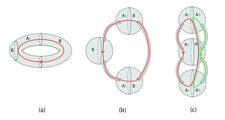
Figure 12: (a) Wave functional $|\Psi\rangle$, which is represented by a tripartite toroidal manifold threaded by a Wilson loop. (b) Deformation of $|\Psi\rangle$, without changing the topology. (c) $\rho_{A_{1}}=\text{tr}_{B}\left(|\Psi\rangle\langle\Psi|\right)$.

This case corresponds to the configuration in Fig. 7 (a). The entanglement entropy $S_{A_{1}\cup A_{2}}$ has already been calculated in Ref. [6], and has the following simple expression

$$S_{A_{1}\cup A_{2}}^{(n)}=2\ln\mathcal{S}_{00}=-2\ln\mathcal{D}.$$ (B.73)

Now we need to calculate $S^{(n)}_{A_{1}}$ (or $S^{(n)}_{A_{2}}$). As shown in Fig. 12, for convenience, we denote the compliment part of $A_{1}$ as $A_{1}^{\complement}=B$. Shown in Fig. 12 (b) is a deformation of $|\Psi\rangle$, based on which we can obtain $\rho_{A_{1}}$ in Fig. 12 (c). Then it can be checked that

$$\text{tr}\left(\rho_{A_{1}}^{n}\right)=\frac{Z(S^{3},\hat{R}_{a})^{2}\cdot Z(S^{3})^{1-n}\cdot Z(S^{3},\hat{R}_{a})^{n}}{Z(S^{3},\hat{R}_{a})^{3n}}=Z(S^{3},\hat{R}_{a})^{2-2n}\cdot Z(S^{3})^{1-n},$$ (B.74)

where we have used Eq. (1.23). Therefore, one has

$$\frac{\text{tr}\left(\rho_{A_{1}}^{n}\right)}{\left(\text{tr}\rho_{A_{1}}\right)^{n}}=\frac{1}{Z(S^{2}\times S^{1},\hat{R}_{a},\hat{\overline{R}}_{a})^{n}}\cdot Z(S^{3},\hat{R}_{a})^{2-2n}\cdot Z(S^{3})^{1-n}=\left(\mathcal{S}_{0a}\right)^{2-2n}\cdot\left(\mathcal{S}_{00}\right)^{1-n}.$$ (B.75)

For the general case $|\Psi\rangle=\sum_{a}\psi_{a}|\hat{R}_{a}\rangle$, it is straightforward to check that

$$\frac{\text{tr}\left(\rho_{A_{1}}^{n}\right)}{\left(\text{tr}\rho_{A_{1}}\right)^{n}}=\frac{\sum_{a}|\psi_{a}|^{2n}Z(S^{3},\hat{R}_{a})^{2-2n}\cdot Z(S^{3})^{1-n}}{\left(\sum_{a}|\psi_{a}|^{2}\right)^{n}}=\sum_{a}|\psi_{a}|^{2n}\left(\mathcal{S}_{0a}\right)^{2-2n}\cdot\left(\mathcal{S}_{00}\right)^{1-n}.$$ (B.76)

Then one has

$$S_{A_{1}}^{(n)} =\frac{1}{1-n}\ln\sum_{a}|\psi_{a}|^{2n}\left(\mathcal{S}_{0a}\right)^{2-2n}+\ln\mathcal{S}_{00},$$

$$\text{and}\quad S_{A_{1}} =2\sum_{a}|\psi_{a}|^{2}\ln\mathcal{S}_{0a}-\sum_{a}|\psi_{a}|^{2}\ln|\psi_{a}|^{2}+\ln\mathcal{S}_{00}.$$ (B.77)

From Fig. 7 (a), it is straightforward to observe that $S_{A_{1}}^{(n)}=S_{A_{2}}^{(n)}$. Then the mutual information between $A_{1}$ and $A_{2}$ has the expression

$$I_{A_{1},A_{2}}^{(n)} =\frac{2}{1-n}\ln\sum_{a}|\psi_{a}|^{2n}\left(\mathcal{S}_{0a}\right)^{2-2n}=\frac{2}{1-n}\ln\sum_{a}|\psi_{a}|^{2n}d_{a}^{2-2n},$$

$$\text{and}\quad I_{A_{1},A_{2}} =2\sum_{a}|\psi_{a}|^{2}\ln\mathcal{S}_{0a}-\sum_{a}|\psi_{a}|^{2}\ln|\psi_{a}|^{2}$$

$$=4\sum_{a}|\psi_{a}|^{2}\ln d_{a}-2\sum_{a}|\psi_{a}|^{2}\ln|\psi_{a}|^{2}-4\ln\mathcal{D}.$$ (B.78)

B.4 Two disjoint non-contractible regions on a torus

This case corresponds to the configuration in Fig. 9 (a). $S_{A_{1}}^{(n)}$ and $S_{A_{2}}^{(n)}$ have the same expression as those in Eq. (B.2.1), and $S_{A_{1}\cup A_{2}}^{(n)}$ is the same as that in Eq. (B.2.2). Therefore, it can be checked that

$$I_{A_{1},A_{2}}^{(n)} =\frac{1}{1-n}\ln\frac{\left(\sum_{a}|\psi_{a}|^{2n}\left(\mathcal{S}_{0a}\right)^{2-2n}\right)^{2}}{\sum_{a}|\psi_{a}|^{2n}\left(\mathcal{S}_{0a}\right)^{4-4n}}=\frac{1}{1-n}\ln\frac{\left(\sum_{a}|\psi_{a}|^{2n}d_{a}^{2-2n}\right)^{2}}{\sum_{a}|\psi_{a}|^{2n}d_{a}^{4-4n}},$$

$$I_{A_{1},A_{2}} =-\sum_{a}|\psi_{a}|^{2}\ln|\psi_{a}|^{2}.$$ (B.79)

It is noted that although $I_{A_{1},A_{2}}$ is independent of the quantum dimension, $I^{(n)}_{A_{1},A_{2}}$ with $n>1$ depends on the quantum dimension explicitly.

References

- [1]
- [2] Alexei Kitaev and John Preskill, “Topological entanglement entropy,” Phys. Rev. Lett. 96, 110404 (2006).
- [3] Michael Levin and Xiao-Gang Wen, “Detecting topological order in a ground state wave function,” Phys. Rev. Lett. 96, 110405 (2006).
- [4] Pasquale Calabrese and John Cardy, “Entanglement entropy and conformal field theory,” Journal of Physics A: Mathematical and Theoretical 42, 504005 (2009).
- [5] J. Eisert, M. Cramer, and M. B. Plenio, “Colloquium : Area laws for the entanglement entropy,” Rev. Mod. Phys. 82, 277–306 (2010).
- [6] S. Dong, E. Fradkin, R. G. Leigh, and S. Nowling, “Topological entanglement entropy in chern-simons theories and quantum hall fluids,” Journal of High Energy Physics 2008, 016 (2008).
- [7] Y. Zhang, T. Grover, A. Turner and M. Oshikawa, and A. Vishwanath, “Quasiparticle statistics and braiding from ground-state entanglement,” Phys. Rev. B 85, 235151 (2012).
- [8] P. Calabrese and J. L. Cardy, “Entanglement entropy and quantum field theory,” J.Stat. Mech. 0406 (2004) P06002
- [9] M. B. Plenio and S. Virmani, “An introduction to entanglement measures,” Quant. Inf. Comput. 7, 1 (2007).
- [10] G. Vidal and R. F. Werner, “Computable measure of entanglement,” Phys. Rev. A 65, 032314 (2002).
- [11] M. B. Plenio, “Logarithmic negativity: A full entanglement monotone that is not convex,” Phys. Rev. Lett. 95, 090503 (2005).
- [12] P. Calabrese, J. Cardy, and E. Tonni, “Entanglement negativity in quantum field theory,” Phys. Rev. Lett. 109, 130502 (2012).
- [13] P. Calabrese, J. Cardy, and E. Tonni, “Entanglement negativity in extended systems: a field theoretical approach,” Journal of Statistical Mechanics: Theory and Experiment 2013, P02008 (2013).
- [14] P. Calabrese, J. Cardy, and E. Tonni, “Finite temperature entanglement negativity in conformal field theory,” J. Phys. A 48, 015006 (2015).
- [15] H. Wichterich, J. Molina-Vilaplana, and S. Bose, “Scaling of entanglement between separated blocks in spin chains at criticality,” Phys. Rev. A 80, 010304(R) (2009). H. Wichterich, J. Vidal, and S. Bose, “ Universality of the negativity in the Lipkin-Meshkov-Glick model, ” Phys. Rev. A 81, 032311 (2010). A. Bayat, S. Bose, and P. Sodano, “Entanglement Routers Using Macroscopic Singlets,” Phys. Rev. Lett. 105, 187204 (2010). A. Bayat, P. Sodano, and S. Bose, “Negativity as the entanglement measure to probe the Kondo regime in the spin-chain Kondo model,” Phys. Rev. B 81, 064429 (2010). A. Bayat, S. Bose, P. Sodano, and H. Johannesson, “Entanglement Probe of Two-Impurity Kondo Physics in a Spin Chain,” Phys. Rev. Lett. 109, 066403 (2012).
- [16] P. Calabrese, L. Tagliacozzo, and E. Tonni, “Entanglement negativity in the critical Ising chain,” J. Stat. Mech. P05002 (2013). P. Ruggiero, V. Alba, and P. Calabrese, “The entanglement negativity in random spin chains,” arXiv:1605.00674.
- [17] K. Audenaert, J. Eisert, M. B. Plenio, and R. F. Werner, “Entanglement properties of the harmonic chain,” Phys. Rev. A 66, 042327 (2002). A. Ferraro, D. Cavalcanti, A. García-Saez, and A. Acin, “Thermal Bound Entanglement in Macroscopic Systems and Area Law,” Phys. Rev. Lett. 100, 080502 (2008). D. Cavalcanti, A. Ferraro, A. García-Saez, and A. Acin, “Distillable entanglement and area laws in spin and harmonic-oscillator systems,” Phys. Rev. A 78, 012335 (2008). J. Anders, “Thermal state entanglement in harmonic lattices,” Phys. Rev. A 77, 062102 (2008). S. Marcovitch, A. Retzker, M. B. Plenio, and B. Reznik, “Critical and noncritical long-range entanglement in Klein-Gordon fields,” Phys. Rev. A 80, 012325 (2009).
- [18] V. Eisler, Z. Zimborás, “Entanglement negativity in two-dimensional free lattice models,” arXiv:1511.08819.
- [19] C. De Nobili, A. Coser and Erik Tonni “Entanglement negativity in a two dimensional harmonic lattice: Area law and corner contributions,” arXiv:1604.02609.
- [20] V. Eisler and Z. Zimboras, “On the partial transpose of fermionic Gaussian states,” New J. Phys. 17 (2015) 053048; arXiv:1502.01369.
- [21] A. Coser, E. Tonni, and P. Calabrese, “Towards entanglement negativity of two disjoint intervals for a one dimensional free fermion,” arXiv:1508.00811. A. Coser, E.Tonni, and P. Calabrese, “Spin structures and entanglement of two disjoint intervals in conformal field theories,” arXiv:1511.08328.
- [22] C. P. Herzog and Yihong Wang, “Estimation for Entanglement Negativity of Free Fermions,” arXiv:1601.00678.
- [23] P.-Y. Chang and X. Wen, “Entanglement negativity in free-fermion systems: An overlap matrix approach,” Phys. Rev. B, 93, 195140 (2016); arXiv:1601.07492.
- [24] Y. A. Lee and G. Vidal, “Entanglement negativity and topological order,” Phys. Rev. A 88, 042318 (2013).
- [25] C. Castelnovo, “Negativity and topological order in the toric code,” Phys. Rev. A 88, 042319 (2013).
- [26] X. Wen, S. Matsuura, and S. Ryu, “Edge theory approach to topological entanglement entropy, mutual information and entanglement negativity in Chern-Simons theories,” arXiv:1603.08534.
- [27] M. Rangamani and M. Rota, “Comments on Entanglement Negativity in Holographic Field Theories,” Journal of High Energy Physics, 2014, 2014:60; arXiv:1406.6989.
- [28] S. Banerjee and P. Paul, “Black Hole Singularity, Generalized (Holographic) c-Theorem and Entanglement Negativity,” arXiv:1512.02232.
- [29] P. Chaturvedi, V. Malvimat and G. Sengupta, “Entanglement negativity, Holography and Black holes,” arXiv:1602.01147.
- [30] V. Eisler and Z. Zimboras, “Entanglement negativity in the harmonic chain out of equilibrium”, New J. Phys. 16 (2014) 123020; arXiv:1406.5474.
- [31] A. Coser, E. Tonni, and P. Calabrese, “Entanglement negativity after a global quantum quench,” J. Stat. Mech. (2014) P12017; arXiv:1410.0900.
- [32] M. Hoogeveen and B. Doyon, “Entanglement negativity and entropy in non-equilibrium conformal field theory,” Nuclear Physics B 898, 78(2015); arXiv:1412.7568.
- [33] X. Wen, P.-Y. Chang and S. Ryu, “Entanglement negativity after a local quantum quench in conformal field theories,” Phys. Rev. B 92, 075109 (2015); arXiv:1501.00568.
- [34] P.Calabrese, J. Cardy and E. Tonni, “Finite temperature entanglement negativity in conformal field theory,” J. Phys. A 48, 015006 (2015); arXiv:1408.3043.
- [35] N. E. Sherman, T. Devakul, M. B. Hastings and Rajiv R. P. Singh, “Nonzero temperature Entanglement Negativity of quantum spin models: Area law, Linked Cluster Expansions and Sudden Death,” Phys. Rev. E 93, 022128 (2016); arXiv:1510.08005.
- [36] D. C. Tsui, H. L. Stormer, and A. C. Gossard, “Two-dimensional magnetotransport in the extreme quantum limit,” Phys. Rev. Lett. 48, 1559–1562 (1982). R. B. Laughlin, “Anomalous quantum hall effect: An incompressible quantum fluid with fractionally charged excitations,” Phys. Rev. Lett. 50, 1395–1398 (1983). X.-G. Wen, “Topological orders and edge excitations in fractional quantum hall states,” Advances in Physics 44, 405–473 (1995).
- [37] X.-G. Wen, “Quantum orders and symmetric spin liquids,” Phys. Rev. B 65, 165113 (2002). L. Savary and L. Balents, “Quantum Spin Liquids,” arXiv:1601.03742.
- [38] N. Read and D. Green, “Paired states of fermions in two dimensions with breaking of parity and time-reversal symmetries and the fractional quantum hall effect,” Phys. Rev. B 61, 10267– 10297 (2000). M. Stone and S.-B. Chung, “Fusion rules and vortices in px + ipy superconductors,” Phys. Rev. B 73, 014505 (2006).
- [39] E. Witten, “Quantum field theory and the jones polynomial,” Communications in Mathematical Physics 121, 351 (1989).
- [40] E. Witten, “On holomorphic factorization of wzw and coset models,” Communications in Mathematical Physics 144, 189 (1992).
- [41] J. Wang, X.-G. Wen and S.-T. Yau, “Quantum Statistics and Spacetime Surgery,” arXiv:1602.05951.
- [42] J. Wang, “Aspects of Symmetry, Topology and Anomalies in Quantum Matter,” arXiv:1602.05569.
- [43] C. M. Jian, I. H. Kim, X. L. Qi, “Long-range mutual information and topological uncertainty principle,” arXiv:1508.07006.