d-wave superconductivity in boson+fermion dimer models

Abstract

We present a slave-particle mean-field study of the mixed boson+fermion quantum dimer model introduced by Punk, Allais, and Sachdev [PNAS 112, 9552 (2015)] to describe the physics of the pseudogap phase in cuprate superconductors. Our analysis naturally leads to four charge $e$ fermion pockets whose total area is equal to the hole doping $p$, for a range of parameters consistent with the $t-J$ model for high temperature superconductivity. Here we find that the dimers are unstable to d-wave superconductivity at low temperatures. The region of the phase diagram with d-wave rather than s-wave superconductivity matches well with the appearance of the four fermion pockets. In the superconducting regime, the dispersion contains eight Dirac cones along the diagonals of the Brillouin zone.

Introduction. The Rokhsar-Kivelson quantum dimer model (QDM) was originally introduced to describe a possible magnetically-disordered phase – the resonating valence bond (RVB) phase – in high-temperature superconducting materials key-1 . The arena where the QDM has been deployed has greatly expanded since its inception, and the model has taken on a key role in the study of a variety of magnetic quantum systems. Quantum dimers show up prominently in the study of hard-core bosons hopping on frustrated lattices key-2 , of arrays of Josephson junctions with capacitative and Josephson couplings key-3 , of frustrated Ising models with an external field or with perturbative XY couplings key-4 , of various types of gauge theories key-5 , and of models with large spin-orbit couplings key-6 and various cold atom setups key-7 . The study of QDMs led to an abundance of new phenomena including deconfined quantum criticality and new routes to deconfinement key-8 . It also provided one of the earliest known examples of topologically ordered states in a lattice model key-25 .

Recently QDMs have been revisited as models of high-temperature superconductivity key-30 ; key-32 ; key-34 . This was motivated by the need to reconcile transport experiments key-44 ; key-45 ; key-46 ; key-29 and photoemission data key-41 ; key-42 ; key-43 in the underdoped region of cuprate superconductors: while photoemission data show Fermi arcs enclosing an area $1+p$ (with $p$ being the doping), transport measurements indicate plain Fermi-liquid properties consistent with an area $p$. In order to resolve this issue and produce a Fermi liquid which encloses an area $p$, the authors of Refs. key-30 ; key-32 ; key-34 introduced a model for the pseudogap region of the cuprate superconductors which consists of two types of dimers: one spinless bosonic dimer – representing a valence bond between two neighboring spins – and one spin $1/2$ fermionic dimer representing a hole delocalized between two sites. Fig. 1 shows an example of a boson+fermion dimer covering of the square lattice and depicts the dimer moves dictated by the quantum Hamiltonian in Eq. (2). The boson+fermion QDM (bfQDM) was introduced and studied numerically in Ref. key-30, using exact diagonalization, supporting the existence of a fractionalized Fermi liquid enclosing an area $p$.

In this work we present a slave boson and fermion formulation of the bfQDM. We find that four symmetric fermion pockets, located in the vicinity of $\left(\pm\frac{\pi}{2},\pm\frac{\pi}{2}\right)$ in the Brillouin zone, naturally appear at mean-field level. The total area of the four pockets is given by the hole (fermionic) doping. We find that the system is unstable to d-wave superconductivity at low temperatures. The region of the phase diagram with d-wave superconductivity matches well the region with four fermion pockets. In the superconducting phase, the fermionic dimers (holes) acquire a Dirac dispersion at eight points along the diagonals of the Brillouin zone.

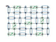
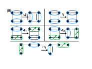
Figure 1: The boson+fermion quantum dimer model of Ref. key-30, . (A) A particular dimer configuration. The lattice is shown in black. The bosonic dimers representing the valence bonds are shown in blue while the spinful fermionic dimers representing a single electron delocalized over two sites are shown in green. (B) Diagrams representative of the various terms in the dimer Hamiltonian Eq. (2).

Mapping onto slave boson/fermion model. The quantum dimer model can be mapped exactly onto a slave boson+fermion model by considering a secondary Hilbert space where we assign to each link ($i,i+\eta$) of the lattice ($\eta=\hat{x},\hat{y}$) a bosonic mode $b_{i,\eta}$ and a spinful fermionic mode $c_{i,\eta,\sigma}$ ($\sigma=\uparrow,\downarrow$). We associate the number of dimers on a link with the occupation numbers of the bosons or fermions on that link. As such we have embedded the dimer Hilbert space in a larger boson/fermion Hilbert space. The constraint that each site of the lattice has one and exactly one dimer attached to it may be rephrased in the boson/fermion language as:

$$\Pi_{i}\equiv\sum_{l\in v_{i}}b_{l}^{\dagger}b_{l}^{\;}+c_{l,\uparrow}^{\dagger}c_{l,\uparrow}^{\;}+c_{l,\downarrow}^{\dagger}c_{l,\downarrow}^{\;}-1=0\,.$$ (1)

Here, for convenience of notation, $\ell\in v_{i}$ labels the four links $j,\eta$ that are attached to vertex $i$. Any Hamiltonian for the dimers has a boson/fermion representation; in particular the terms illustrated in Fig. 1B can be written as:

$$H_{D}= \sum_{i}\left\{-J\,b_{i,\hat{x}}^{\dagger}b_{i+\hat{y},\hat{x}}^{\dagger}b_{i,\hat{y}}^{\;}b_{i+\hat{x},\hat{y}}^{\;}+1\>\text{term}\right.$$

$$\left.+V\,b_{i,\hat{x}}^{\dagger}b_{i,\hat{x}}^{\;}b_{i+\hat{y},\hat{x}}^{\dagger}b_{i+\hat{y},\hat{x}}^{\;}+1\>\text{term}\right\}$$

$$\sum_{i}\sum_{\sigma}\left\{-t_{1}\,b_{i,\hat{x}}^{\dagger}c_{i+\hat{y},\hat{x},\sigma}^{\dagger}c_{i,\hat{x},\sigma}^{\;}b_{i+\hat{y},\hat{x}}^{\;}+3\>\text{terms}\right.$$

$$-t_{2}\,b_{i+\hat{x},\hat{y}}^{\dagger}c_{i,\hat{y},\sigma}^{\dagger}c_{i,\hat{x},\sigma}^{\;}b_{i+\hat{y},\hat{x}}^{\;}+7\>\text{terms}$$

$$-t_{3}\,b_{i+\hat{x}+\hat{y},\hat{x}}^{\dagger}c_{i,\hat{y},\sigma}^{\dagger}c_{i+\hat{x}+\hat{y},\hat{x},\sigma}^{\;}b_{i,\hat{y}}^{\;}+7\>\text{terms}$$

$$\left.-t_{3}\,b_{i+2\hat{y},\hat{x}}^{\dagger}c_{i,\hat{y},\sigma}^{\dagger}c_{i+2\hat{y},\hat{x},\sigma}^{\;}b_{i,\hat{y}}^{\;}+7\>\text{terms}\right\}$$

$$-\mu\sum_{i}\sum_{\sigma}\sum_{\eta}c_{i,\eta,\sigma}^{\dagger}c_{i,\eta,\sigma}^{\;}\,,$$ (2)

where we included a chemical potential for the holes (fermionic dimers), which is important for the connection with doped high-temperature superconductors key-40 ; key-48 . The terms not written explicitly in Eq. (2) are simply obtained from those shown by translational symmetry, four fold rotational symmetry, and reflection symmetry about the two diagonals. This Hamiltonian also has a local $U\left(1\right)$ gauge symmetry

$$b_{i,\eta}\rightarrow e^{i\theta_{i}}\;b_{i,\eta}\;e^{i\theta_{i+\eta}}\;,\quad c_{i,\eta,\sigma}\rightarrow e^{i\theta_{i}}\;c_{i,\eta,\sigma}\;e^{i\theta_{i+\eta}}\;,$$ (3)

with a phase $\theta_{i}$ associate to each vertex $i$. Any Hamiltonian that preserves the constraint given in Eq. (1) is invariant under this gauge transformation key-31 ; key-33 (23).

A slave boson/fermion formulation of the bfQDM is obtained by introducing a Lagrange multiplier: a real field $\lambda_{i}(\tau)$ that enforces the dimer constraint Eq. (1) at all times $\tau$, and shifting the action by $\Delta{\cal S}=-\int d\tau\sum_{i}\lambda_{i}(\tau)\,\Pi_{i}(\tau)$.

Slave boson/fermion mean-field decoupling. A systematic mean-field approach can be obtained by taking the saddle point with respect to the Lagrange multiplier field $\lambda_{i}(\tau)\to\lambda_{i}$, with a time-independent value $\lambda_{i}$ that enforces the average constraint $\langle\Pi_{i}\rangle=0$. This procedure is accompanied by Hubbard Stratonovich (HS) transformations of every term in the Hamiltonian in Eq. (2) separately. We begin with the purely bosonic potential term:

$$b_{i,\hat{x}}^{\dagger}b_{i,\hat{x}}^{\;}b_{i+\hat{y},\hat{x}}^{\dagger}b_{i+\hat{y},\hat{x}}^{\;}\rightarrow$$

$$\>\kappa_{1}\left\{b_{i,\hat{x}}^{\dagger}b_{i,\hat{x}}^{\;}\,x_{i1}+b_{i+\hat{y},\hat{x}}^{\dagger}b_{i+\hat{y},\hat{x}}^{\;}\,x_{i2}-x_{i1}x_{i2}\right\}$$

$$+\left(1-\kappa_{1}\right)\left\{b_{i,\hat{x}}^{\dagger}b_{i+\hat{y},\hat{x}}^{\dagger}\,z_{i}+b_{i,\hat{x}}^{\;}b_{i+\hat{y},\hat{x}}^{\;}\,z_{i}^{*}-\left|z_{i}^{2}\right|\right\},$$ (4)

where $x_{i}$ and $z_{i}$ are auxiliary fields to be integrated over and $\kappa_{1}$ is arbitrary. At mean-field level we can drop the integrals over the auxiliary fields and replace them with their saddle point values $x_{i1}\rightarrow\langle b_{i+\hat{y},\hat{x}}^{\dagger}b_{i+\hat{y},\hat{x}}^{\;}\rangle$, $x_{i2}\rightarrow\langle b_{i,\hat{x}}^{\dagger}b_{i,\hat{x}}^{\;}\rangle$ and $z_{i}\rightarrow\langle b_{i,\hat{x}}^{\;}b_{i+\hat{y},\hat{x}}^{\;}\rangle$. The hopping term may be decoupled in a similar manner:

$$b_{i,\hat{x}}^{\dagger}b_{i+\hat{y},\hat{x}}^{\dagger}b_{i,\hat{y}}^{\;}b_{i+\hat{x},\hat{y}}^{\;}+\text{h.c.}\rightarrow$$

$$\>\kappa_{2}\left\{b_{i,\hat{x}}^{\dagger}b_{i+\hat{y},\hat{x}}^{\dagger}\,w_{i1}+b_{i,\hat{y}}^{\;}b_{i+\hat{x},\hat{y}}^{\;}\,w_{i2}^{*}-w_{i1}w_{i2}^{*}+\text{h.c.}\right\}$$

$$+\left(1-\kappa_{2}\right)\left\{b_{i,\hat{x}}^{\dagger}b_{i,\hat{y}}^{\;}\,q_{i1}+b_{i+\hat{y},\hat{x}}^{\dagger}b_{i+\hat{x},\hat{y}}^{\;}\,q_{i2}^{*}-q_{i1}q_{i2}^{*}+\text{h.c.}\right\},$$ (5)

where, again, at mean-field level we use the saddle point values $w_{i1}\rightarrow\langle b_{i,\hat{y}}^{\;}b_{i+\hat{x},\hat{y}}^{\;}\rangle$, $w_{i2}^{*}\rightarrow\langle b_{i,\hat{x}}^{\dagger}b_{i+\hat{y},\hat{x}}^{\dagger}\rangle$, $q_{i1}\rightarrow\langle b_{i+\hat{y},\hat{x}}^{\dagger}b_{i+\hat{x}^{\;},\hat{y}}\rangle$, $q_{i2}^{*}\rightarrow\langle b_{i,\hat{x}}^{\dagger}b_{i,\hat{y}}\rangle$ and $\kappa_{2}$ is arbitrary. Other HS decouplings, and linear combinations thereof, are also possible.

We can make substantial progress in understanding the fermionic component of the theory without detailed analysis of the bosonic component. Indeed, any translationally invariant (liquid-like) bosonic ansatz, naturally expected in $U\left(1\right)$ gauge theories coupled to fermions with a Fermi surface key-37 (24, 25, 26), yields similar fermionic effective theories. The fermionic mean-field Hamiltonian reads

$$H_{F\bar{B}} =\sum_{\sigma}\sum_{i}\left\{-t_{1}\;c_{i+\hat{y},\hat{x},\sigma}^{\dagger}c_{i,\hat{x},\sigma}^{\;}\langle b_{i,\hat{x}}^{\dagger}b_{i+\hat{y},\hat{x}}^{\;}\rangle+3\;\text{terms}\right.$$

$$-t_{2}\;c_{i,\hat{y},\sigma}^{\dagger}c_{i,\hat{x},\sigma}^{\;}\langle b_{i+\hat{x},\hat{y}}^{\dagger}b_{i+\hat{y},\hat{x}}^{\;}\rangle+7\;\text{terms}$$

$$-t_{3}\;c_{i,\hat{y},\sigma}^{\dagger}c_{i+\hat{x}+\hat{y},\hat{x},\sigma}^{\;}\langle b_{i+\hat{x}+\hat{y},\hat{x}}^{\dagger}b_{i,\hat{y}}^{\;}\rangle+7\;\text{terms}$$

$$\left.-t_{3}\;c_{i,\hat{y},\sigma}^{\dagger}c_{i+2\hat{y},\hat{x},\sigma}^{\;}\langle b_{i+2\hat{y},\hat{x}}^{\dagger}b_{i,\hat{y}}^{\;}\rangle+7\;\text{terms}\right\}$$

$$\left(-2\lambda-\mu\right)\sum_{i}\sum_{\sigma}\sum_{\eta}c_{i,\eta,\sigma}^{\dagger}c_{i,\eta,\sigma}^{\;}\;,$$ (6)

which is effectively a tight-biding model with renormalized hoppings $T_{1}=t_{1}\;\langle b_{i,\hat{x}}^{\dagger}b_{i+\hat{y},\hat{x}}^{\;}\rangle$, $T_{2}=t_{2}\;\langle b_{i+\hat{x},\hat{y}}^{\dagger}b_{i+\hat{y},\hat{x}}^{\;}\rangle$ and $T_{3}=t_{3}\;\langle b_{i+\hat{x}+\hat{y},\hat{x}}^{\dagger}b_{i,\hat{y}}^{\;}\rangle$.

The resulting model is defined on the bipartite checkerboard lattice that is medial to the original square lattice. The horizontal ($x$) and vertical ($y$) links make up the two sublattices where the fermions reside. We define (in momentum space) the spinor that encodes these two flavors as $\psi_{\vec{k},\sigma}^{\dagger}=(c_{\vec{k},\hat{y},\sigma}^{\dagger},c_{\vec{k},\hat{x},\sigma}^{\dagger})$ and

$$H_{F\bar{B}}=\sum_{\vec{k},\sigma}\psi_{\vec{k},\sigma}^{\dagger}\,\begin{pmatrix}\xi_{\vec{k}}^{x}&\gamma_{\vec{k}}\\ \gamma_{\vec{k}}^{*}&\xi_{\vec{k}}^{y}\end{pmatrix}\;\psi_{\vec{k},\sigma}\;,$$ (7)

where:

$$\xi_{\vec{k}}^{x} =-2\lambda-\mu-2\,T_{1}\;\cos k_{x}\;$$

$$\xi_{\vec{k}}^{y} =-2\lambda-\mu-2\,T_{1}\;\cos k_{y}\;$$

$$\gamma_{\vec{k}} =4e^{i(k_{y}-k_{x})/2}\;\left(T_{2}\;\cos\frac{k_{x}}{2}\cos\frac{k_{y}}{2}\right.$$

$$\left.+T_{3}\;\cos\frac{3k_{x}}{2}\cos\frac{k_{y}}{2}+T_{3}\;\cos\frac{k_{x}}{2}\cos\frac{3k_{y}}{2}\right).$$

The eigenvalues are given by $E_{\pm,\vec{k}}=\xi_{\vec{k}}\pm\sqrt{\eta_{\vec{k}}^{2}+|\gamma_{\vec{k}}|^{2}}$, where $\xi_{\vec{k}}=(\xi_{\vec{k}}^{x}+\xi_{\vec{k}}^{y})/2$ and $\eta_{\vec{k}}=(\xi_{\vec{k}}^{x}-\xi_{\vec{k}}^{y})/2$. For hole doping $p$ (the number of fermions in our model) the lower band $E_{-,\vec{k}}$ will be partially occupied. The total area enclosed by the Fermi surface in the lower band is equal to the hole doping $p$ (multiplied by $4\pi^{2}$).

The Hamiltonian Eq. (7) has four-fold rotational symmetry, $k_{x}\rightarrow k_{y}$ and $k_{y}\rightarrow-k_{x}$, and reflection symmetry about the diagonals $k_{x}\rightarrow k_{y}$ and $k_{y}\rightarrow k_{x}$ as well as $k_{x}\rightarrow-k_{y}$ and $k_{y}\rightarrow-k_{x}$. Depending on the relative values of $T_{1}$, $T_{2}$ and $T_{3}$, the band minima will be located at different points in the Brillouin zone, and the Fermi surface topology will vary accordingly. In Fig. 2A we show the position of the minima along the $k_{x}=\pm k_{y}$ directions (or $\Gamma-M$ line), as a function of the ratios $T_{3}/T_{1}$ and $T_{2}/T_{1}$. We identify two regions in parameter space, where the dispersion minima are (i) at the $\Gamma$ point (blue-colored region), and (ii) in between the $\Gamma$ and $M$ points, varying continuously with $T_{1}/T_{3}-T_{2}/T_{3}$ (faded region). An example of dispersion where the minima are at $(k_{x},k_{y})\simeq(\pm\pi/2,\pm\pi/2)$ is shown in the bottom inset of Fig. 2A. Case (ii) is clearly conducive to the appearance of four Fermi pockets in an appropriate range of the chemical potential.

Figure 2: (A) Location of the band minima as a function of $T_{3}/T_{1}$ and $T_{2}/T_{1}$. The color scale corresponds to the distance along the $\Gamma-M$ line in the Brillouin zone: blue corresponds to the $\Gamma$ point, $k_{x}=k_{y}=0$, and red corresponds to the $M$ point, $k_{x}=k_{y}=\pi$. The insets show contours of the dispersion of the lower band of the Hamiltonian Eq. (6) for specific choices of parameters in the corresponding regions. (B) Dominant superconductivity instability as a function of $T_{3}/T_{1}$ and $T_{2}/T_{1}$ for doping $p=0.25$ and $J=50$: d-wave (white) vs. s-wave (black). Note the good correlation between d-wave superconductivity and the appearance of four band minima.

d-wave Superconductivity. To study superconducting instabilities we need to include four-fermion terms in the Hamiltonian, i.e., go beyond the model introduced in Refs. key-30, ; key-32, ; key-34, and summarized in Fig. 1B and Eq. (2). Consider the $t-J$ Hamiltonian on the square lattice key-36 (27),

$$H_{tJ}=-\sum_{\alpha}t_{ij}d_{i,\alpha}^{\dagger}d_{j,\alpha}^{\;}+J\sum_{\left\langle i,j\right\rangle}\left(\vec{S}_{i}\cdot\vec{S}_{j}-\frac{1}{4}n_{i}n_{j}\right)$$ (8)

subject to the constraint that $n_{i}\leq 1$. Here $d_{i,\alpha}^{\dagger}$ and $d_{i,\alpha}^{\ }$ are the electron creation and annihilation operators ($\alpha=\uparrow,\downarrow$) of the $t-J$ model, $\vec{S}_{i}=d_{i,\alpha}^{\dagger}\,\vec{\sigma}_{\alpha,\beta}\,d_{i,\beta}^{\ }$ (with $\alpha,\,\beta$ summed over), and $n_{i}=d_{i,\uparrow}^{\dagger}d_{i,\uparrow}^{\ }+d_{i,\downarrow}^{\dagger}d_{i,\downarrow}^{\ }$.

We can identify the dimer Hilbert space with a subspace of the Hilbert space for the $t-J$ model, where the zero dimers state corresponds to the state with zero electrons, and the rest of the Hilbert space can be introduced via the operators $b_{i,\eta}^{\dagger}\Leftrightarrow\Upsilon_{i,\eta}\,(d_{i\uparrow}^{\dagger}d_{i+\eta\downarrow}^{\dagger}-d_{i\downarrow}^{\dagger}d_{i+\eta\uparrow}^{\dagger})/\sqrt{2}$ and $c_{i,\eta,\sigma}^{\dagger}\Leftrightarrow\Upsilon_{i,\eta}(d_{i,\sigma}^{\dagger}+d_{i+\eta,\sigma}^{\dagger})/\sqrt{2}$. The phases $\Upsilon_{i,\eta}$ represent a gauge choice and we shall follow the one by Rokhsar and Kivelson key-1 and define $\Upsilon_{i,\hat{y}}=1$ and $\Upsilon_{i,\hat{x}}=\left(-1\right)^{i_{y}}$, where $i_{y}$ is the $y$-component of the 2D square lattice site index $i$.

Given the conventional inner product for the electron Hilbert space, the dimer basis is not orthonormal. This issue can be addressed in general by Gram-Schmidt orthogonalization key-35 (28); however, it is customary to use the leading order approximation and to assume that the dimer states are orthogonal (and normalized) key-33 (23). The relevant Hamiltonian can then be determined by projecting Eq. (8) onto this basis. The pairing term (four-fermion interaction) comes from the spin-spin term in the $t-J$ model, namely $H_{J}=J\sum_{\langle i,j\rangle}\left(\vec{S}_{i}\cdot\vec{S}_{j}-\frac{1}{4}n_{i}n_{j}\right)$. Let us focus on a single plaquette term and consider eight relevant states for this plaquette, $c_{i,\hat{x},\alpha}^{\dagger}c_{i+\hat{y},\hat{x},\beta}^{\dagger}\left|0\right\rangle$ and $c_{i,\hat{y},\alpha}^{\dagger}c_{i+\hat{x},\hat{y},\beta}^{\dagger}\left|0\right\rangle$, $\alpha,\,\beta=\uparrow,\downarrow$. The Hamiltonian $H_{J}$ is non-zero only in the singlet channel and therefore we must restrict the spins $\alpha,\beta$ to be in a singlet state, thereby the effective Hamiltonian for the dimers is given by $\tilde{H}_{J}=\left(\begin{smallmatrix}-J/2&0\\ 0&-J/2\end{smallmatrix}\right)$ key-33 (23). As such we add to our Hamiltonian in Eq. (2) the term:

$$\tilde{H}_{J} =-\frac{J}{4}\sum_{i}\left(\epsilon_{\alpha\gamma}\,c_{i,\hat{x},\alpha}^{\dagger}\,c_{i+\hat{y},\hat{x},\gamma}^{\dagger}\right)\left(\epsilon_{\beta\delta}\,c_{i+\hat{y},\hat{x},\beta}^{\phantom{\dagger}}\,c_{i,\hat{x},\delta}^{\phantom{\dagger}}\right)$$

$$+x\leftrightarrow y\,.$$ (9)

For convenience we define $\Delta_{x}=\epsilon_{\alpha\gamma}\langle c_{i,\hat{y},\alpha}^{\dagger}\,c_{i+\hat{x},\hat{y},\gamma}^{\dagger}\rangle$ and $\Delta_{y}=\epsilon_{\alpha\gamma}\langle c_{i,\hat{x},\alpha}^{\dagger}\,c_{i+\hat{y},\hat{x},\gamma}^{\dagger}\rangle$, whereby d-wave pairing corresponds to $\Delta_{x}=-\Delta_{y}=\Delta$ (which in turn can be chosen real with an appropriate choice of phase). Using a HS transformation on Eq. (9), $H=\sum_{\vec{k}}\Psi_{\vec{k}}^{\dagger}\;{\cal H}_{\vec{k}}\;\Psi_{\vec{k}}^{\;}$, where

$${\cal H}_{\vec{k}}=\begin{pmatrix}\xi_{\vec{k}}^{x}&\gamma_{\vec{k}}&\Delta_{\vec{k}}^{x}&0\\ \gamma_{\vec{k}}^{*}&\xi_{\vec{k}}^{y}&0&\Delta_{\vec{k}}^{y}\\ \Delta_{\vec{k}}^{x}&0&-\xi_{-\vec{k}}^{x}&-\gamma_{-\vec{k}}\\ 0&\Delta_{\vec{k}}^{y}&-\gamma_{-\vec{k}}^{*}&-\xi_{-\vec{k}}^{y}\;,\end{pmatrix}$$ (10)

and $\Psi_{\vec{k}}^{\dagger}=(c_{\vec{k},\hat{y},\uparrow}^{\dagger},c_{\vec{k},\hat{x},\uparrow}^{\dagger},c_{-\vec{k},\hat{y},\downarrow}^{\;},c_{-\vec{k},\hat{x},\downarrow}^{\;})$. Here $\Delta_{\vec{k}}^{x}=\frac{J}{2}\Delta_{x}\cos k_{x}$ and $\Delta_{\vec{k}}^{y}=\frac{J}{2}\Delta_{y}\cos k_{y}$. The eigenvalues of this Hamiltonian are given by

$$E_{\pm,\pm,{\vec{k}}}=\pm\sqrt{\Theta_{\vec{k}}\pm\sqrt{\Lambda_{\vec{k}}+\Xi_{\vec{k}}}}$$ (11)

where

$$\Theta_{\vec{k}} =\frac{1}{2}\left[(\xi_{\vec{k}}^{x})^{2}+(\xi_{\vec{k}}^{y})^{2}+(\Delta_{\vec{k}}^{x})^{2}+(\Delta_{\vec{k}}^{y})^{2}+2|\gamma_{\vec{k}}|^{2}\right]$$

$$\Lambda_{\vec{k}} =\frac{1}{4}\left[(\xi_{\vec{k}}^{x})^{2}-(\xi_{\vec{k}}^{y})^{2}+(\Delta_{\vec{k}}^{x})^{2}-(\Delta_{\vec{k}}^{y})^{2}\right]^{2}$$

$$\Xi_{\vec{k}} =|\gamma_{\vec{k}}|^{2}\left[(\xi_{\vec{k}}^{x}+\xi_{\vec{k}}^{y})^{2}+(\Delta_{\vec{k}}^{x}-\Delta_{\vec{k}}^{y})^{2}\right].$$

When $T_{1}$, $T_{2}$ and $T_{3}$ are such that there are four Fermi pockets (in the absence of superconductivity), there are eight Dirac points in the dispersion, i.e., there are eight nodes where the gap $E_{+,-,{\vec{k}}}=E_{-,-,{\vec{k}}}=0$. These points are located along the diagonals of the Brillouin zone. When $k_{x}=\pm k_{y}$, $\Lambda_{\vec{k}}$ vanishes, and the gap closing condition $\Theta_{\vec{k}}=\sqrt{\Xi_{\vec{k}}}$ is equivalent to $\xi_{{\vec{k}}}^{2}+\Delta_{{\vec{k}}}^{2}-|\gamma_{\vec{k}}|^{2}=0$, where $\xi_{\vec{k}}=(\xi_{\vec{k}}^{x}+\xi_{\vec{k}}^{y})/2$ and $\Delta_{\vec{k}}=(\Delta_{\vec{k}}^{x}-\Delta_{\vec{k}}^{y})/2$. Notice that the Fermi surface in the absence of superconductivity is given by $\xi_{{\vec{k}}}^{2}-|\gamma_{\vec{k}}|^{2}=0$. Therefore, whenever there are four Fermi pockets, for a range of $\Delta_{{\vec{k}}}^{2}$ there will be two nodes for each pocket, slightly shifted along the diagonal from the original Fermi surface key-33 (23).

Using self consistent equations for the superconducting order parameter, we can then compare s-wave and d-wave instabilities. Up to an unimportant constant energy shift, the Gibbs free energy is given by

$$G =\frac{J}{4}\left(\left|\Delta_{x}^{2}\right|+\left|\Delta_{y}^{2}\right|\right)$$ (12)

$$-\frac{2}{\beta}\int\frac{d^{2}k}{4\pi^{2}}\ln\left[\cosh\left(\frac{\beta}{2}E_{+,+,\vec{k}}\right)\cosh\left(\frac{\beta}{2}E_{+,-,\vec{k}}\right)\right].$$

Minimizing the free energy with respect to $\Delta_{x}$, we obtain:

$$\Delta_{x} \!=\!\!\sum_{s=\pm}\int\frac{d^{2}k}{4\pi^{2}}\;\frac{\tanh\left(\frac{\beta}{2}E_{+,s,\vec{k}}\right)\cos\left(k_{x}\right)}{2{E}_{+,s,\vec{k}}}$$ (13)

$$\!\!\times\left\{\Delta_{\vec{k}}^{x}+\frac{s}{\sqrt{\Lambda_{\vec{k}}+\Xi_{\vec{k}}}}\left[\sqrt{\Lambda_{\vec{k}}}\;\Delta_{\vec{k}}^{x}+\left|\gamma_{\vec{k}}\right|^{2}\left(\Delta_{\vec{k}}^{x}-\Delta_{\vec{k}}^{y}\right)\right]\right\}$$

and similarly for $\Delta_{y}$. From the symmetries of this equation we see that there are two solutions, $\Delta_{x}=\mp\Delta_{y}$, corresponding to d-wave and extended s-wave superconductivity.

We numerically compare the two solutions at zero temperature and find that d-wave superconductivity wins for a large range of ratios $T_{2}/T_{1}$ and $T_{3}/T_{1}$, as illustrated in Fig. 2B. The correlation between the region with fermion pockets depicted in Fig 2A and the region with d-wave superconductivity in Fig. 2B is evident. This can be qualitatively understood as the largest change in the Gibbs free energy upon entering the superconducting state comes from the contribution of the integral around the FS. Since the shape of the four Fermi pockets follows largely the nodal lines of the s-wave order parameter, and it anti-correlates with the d-wave nodal lines, one expects the appearance of the pockets to favor d-wave superconductivity.

Whereas the horizontal boundaries match very well in the two panels in Fig. 2, the vertical boundaries less so. Indeed, along the horizontal boundary the dispersion transitions smoothly from having a single minimum at the $\Gamma$ point to having four minima along the $\Gamma-M$ direction in the Brillouin zone, i.e., the minima move continuously away from the $\Gamma$ point (which thus becomes a maximum). On the other hand, along the vertical boundary, the minima jump discontinuously from the $\Gamma$ point to the new four minima, as four local minima at finite momenta dip down to become the global minima. Depending on the value of the chemical potential, there is a region in the $T_{2}/T_{1}$ vs. $T_{3}/T_{1}$ plane near the vertical boundary where the Fermi surface has five sheets, four pockets coexisting with a surface surrounding the $\Gamma$ point. The latter favors s-wave superconductivity as it has no nodes at the $\Gamma$ point, and it is therefore expected to shift the position of the boundary between d-wave and s-wave superconductivity, as observed.

Conclusions. We presented a slave particle formulation of a mixed boson+fermion quantum dimer model recently proposed in the context of high-T_c superconductors key-30 ; key-32 ; key-34 . A key finding of this work is that substantial progress can be made using a mean-field analysis that simply assumes a translational and rotational invariant (liquid) state for the bosonic component. We analyze the effective theory for the remaining fermionic degrees of freedom, and distinguish between two regimes of Fermi surface topology, depending on the effective couplings obtained from both microscopic parameters and correlations of the bosonic liquid state. The two regimes correspond to one Fermi surface around the $\Gamma$ point, or four Fermi pockets centered along the $\Gamma-M$ lines. By including additional interactions that arise from the $t-J$ model, we find that the system is unstable to superconductivity. The symmetry of the superconducting order parameter, s-wave vs. d-wave, is shown to correlate strongly with the Fermi surface topology, with d-wave being favored when four Fermi pockets are present.

Acknowledgements: This work was supported in part by Engineering and Physical Sciences Research Council (EPSRC) Grants No. EP/G049394/1 (C.Ca.) and No. EP/M007065/1 (C.Ca. and G.G.), by DOE Grant DEF-06ER46316 (C.Ch.), and by the EPSRC Network Plus on “Emergence and Physics far from Equilibrium”. Statement of compliance with the EPSRC policy framework on research data: this publication reports theoretical work that does not require supporting research data. C.Ca. and G.G. thank the BU visitor program for its hospitality.

Supplementary Online Information

I Effective Hamiltonian

Here we provide more details about the derivation of the effective two body (four fermion) interaction introduced in Eq. (9) in the main text. The procedure to obtain this term for the dimer model is to identify the dimer Hilbert space with a subspace of the $t-J$ model Hilbert space and project the $t-J$ Hamiltonian Eq. (8) accordingly.

We identify the state with zero dimers of any kind with the state with zero electrons for the $t-J$ model. The rest of the Hilbert space for the dimers can be introduced via the operators $b_{i,\eta}^{\dagger}\Leftrightarrow\Upsilon_{i,\eta}\,(d_{i\uparrow}^{\dagger}d_{i+\eta\downarrow}^{\dagger}-d_{i\downarrow}^{\dagger}d_{i+\eta\uparrow}^{\dagger})/\sqrt{2}$ and $c_{i,\eta,\sigma}^{\dagger}\Leftrightarrow\Upsilon_{i,\eta}(d_{i,\sigma}^{\dagger}+d_{i+\eta,\sigma}^{\dagger})/\sqrt{2}$. The phases $\Upsilon_{i,\eta}$ represent a gauge choice and we shall follow the one by Rokhsar and Kivelson key-1-1 (1) and define $\Upsilon_{i,\hat{y}}=1$ and $\Upsilon_{i,\hat{x}}=\left(-1\right)^{i_{y}}$, here $i_{y}$ is the y-component of the dimer co-ordinate. Given the conventional inner product for the electron Hilbert space, the dimer basis is not orthonormal and therefore does not serve as a convenient basis to calculate matrix elements. This can be resolved by Gram-Schmidt orthogonalization. In general, if we denote the basis elements of the dimer Hilbert space by $|A\rangle$ and the overlap matrix between states $S_{AB}=\langle A|B\rangle$, then an orthonormal basis for the Hilbert space is given by key-35-1 (2):

$$|\tilde{A}\rangle=\sum_{A}\left(S^{-1/2}\right)_{A,\tilde{A}}|A\rangle.$$ (14)

It is not too hard to check that the matrix $S$ is a real symmetric matrix $S_{AB}=S_{BA}$ and therefore $S^{\dagger}=S$. From this it follows that $\left\langle\tilde{A}\mid\tilde{B}\right\rangle=S^{-1/2}SS^{-1/2}=\delta_{\tilde{A},\tilde{B}}$, i.e., the new states are orthonormal.

The Hamiltonian projected onto this basis is given by key-35-1 (2):

$$H_{\tilde{A},\tilde{B}}=\sum_{A,B}(S^{-1/2})_{\tilde{A},A}\;\langle A|H_{tJ}|B\rangle\;(S^{-1/2})_{B,\tilde{B}}.$$ (15)

To leading order, $S_{AB}\simeq\delta_{A,B}$ as the dimers are nearly orthogonal. To show this consider two states $\left|A\right\rangle$ and $\left|B\right\rangle$. We can form the loop graph of $\left|A\right\rangle$ and $\left|B\right\rangle$ by deleting all the dimers that $\left|A\right\rangle$ and $\left|B\right\rangle$ have in common. The rest of the dimers will form loops (with dimers from state $\left|A\right\rangle$ and state $\left|B\right\rangle$ alternating along a loop). If there is a loop of length 2, that is two dimers of different type on the same link then $\left\langle A\mid B\right\rangle=0$, so we have $S_{AB}=\delta_{A,B}$ for those states. Assuming there are no such links we have that all loops are at least length four. Now the overlap of $\left|A\right\rangle$ and $\left|B\right\rangle$ is the product of overlaps over all loops. Furthermore it is known that the overlap between two loops is exponential in the length of the loop key-1-1 (1, 2). Since all loops are of at least length four (rather long) to leading order we may set the overlap matrix to zero if there is at least one loop or the states $\left|A\right\rangle$ and $\left|B\right\rangle$ are different. Now the states are normalized to unity so we have $S_{AB}\simeq\delta_{A,B}$.

The pairing term (four-fermion interaction) comes from the spin-spin term in the $t-J$ model, namely $H_{J}=J\sum_{\langle i,j\rangle}\left(\vec{S}_{i}\cdot\vec{S}_{j}-\frac{1}{4}n_{i}n_{j}\right)$. Let us focus on a single plaquette term and consider eight relevant states for the dimers on this plaquette, $c_{i,\hat{x},\alpha}^{\dagger}c_{i+\hat{y},\hat{x},\beta}^{\dagger}\left|0\right\rangle$ and $c_{i,\hat{y},\alpha}^{\dagger}c_{i+\hat{x},\hat{y},\beta}^{\dagger}\left|0\right\rangle$. We notice that the Hamiltonian $H_{J}$ is zero in the triplet channel. This means that the effective Hamiltonian for the dimers $\tilde{H}_{J}$ is also zero in the triplet channel. Indeed, the spins of the dimers are the same as the spins of the electrons for the $t-J$ model, so the projected Hamiltonian has the same spin structure. As such we might as well restrict the spins of the dimers to lie in a singlet (there are two such states per plaquette with the two dimers lying either along the x-axis or along the y-axis). Moreover, the projected Hamiltonian is diagonal in this basis. Indeed the bare Hamiltonian $H_{J}$ contains no hopping terms for the electrons, only spin flip terms. As such the only terms that could contribute to off diagonal matrix elements come from states of the form $d_{i,\alpha}^{\dagger}d_{i+\hat{x}+\hat{y},\beta}^{\dagger}\left|0\right\rangle$ and $d_{i+\hat{x},\alpha}^{\dagger}d_{i+\hat{y},\beta}^{\dagger}\left|0\right\rangle$ (and linear combinations thereof) which belong to both dimer configurations (along the x-axis and along the y-axis). However the Hamiltonian annihilates such states and the projected Hamiltonian has no corresponding hopping terms. By symmetry the Hamiltonian when restricted to the singlet subspace is a multiple of the identity matrix. Its value is given by:

$$2\left\langle 0\right|\frac{1}{2\sqrt{2}}\left\{\left(d_{i,\uparrow}+d_{i+\hat{x},\uparrow}\right)\left(d_{i+\hat{y},\downarrow}+d_{i+\hat{y}+\hat{x},\downarrow}\right)-\left(d_{i,\downarrow}+d_{i+\hat{x},\downarrow}\right)\left(d_{i+\hat{y},\uparrow}+d_{i+\hat{y}+\hat{x},\uparrow}\right)\right\}J\left(\vec{S}_{i}\cdot\vec{S}_{i+\hat{y}}-\frac{1}{4}n_{i}n_{i+\hat{y}}\right)$$

$$\left\{\left(d_{i+\hat{y},\downarrow}^{\dagger}+d_{i+\hat{y}+\hat{x},\downarrow}^{\dagger}\right)\left(d_{i,\uparrow}^{\dagger}+d_{i+\hat{x},\uparrow}^{\dagger}\right)-\left(d_{i+\hat{y},\uparrow}^{\dagger}+d_{i+\hat{y}+\hat{x},\uparrow}^{\dagger}\right)\left(d_{i,\downarrow}^{\dagger}+d_{i+\hat{x},\downarrow}^{\dagger}\right)\right\}\frac{1}{2\sqrt{2}}\left|0\right\rangle=-\frac{J}{2}$$

and, within the spin-singlet channel, the Hamiltonian is $\tilde{H}_{J}=\left(\begin{smallmatrix}-J/2&0\\ 0&-J/2\end{smallmatrix}\right)$. Correspondingly, we can add to our Hamiltonian in Eq. (2) the term:

$$\tilde{H}_{J} =-\frac{J}{4}\sum_{i}\left(\epsilon_{\alpha\gamma}\;c_{i,\hat{x},\alpha}^{\dagger}\,c_{i+\hat{y},\hat{x},\gamma}^{\dagger}\right)\left(\epsilon_{\beta\delta}c_{i+\hat{y},\hat{x},\beta}^{\phantom{\dagger}}\,c_{i,\hat{x},\delta}^{\phantom{\dagger}}\right)$$

$$+x\leftrightarrow y\,.$$ (16)

This is a spin spin Hamiltonian for the fermionic dimers.

II Dirac Cones

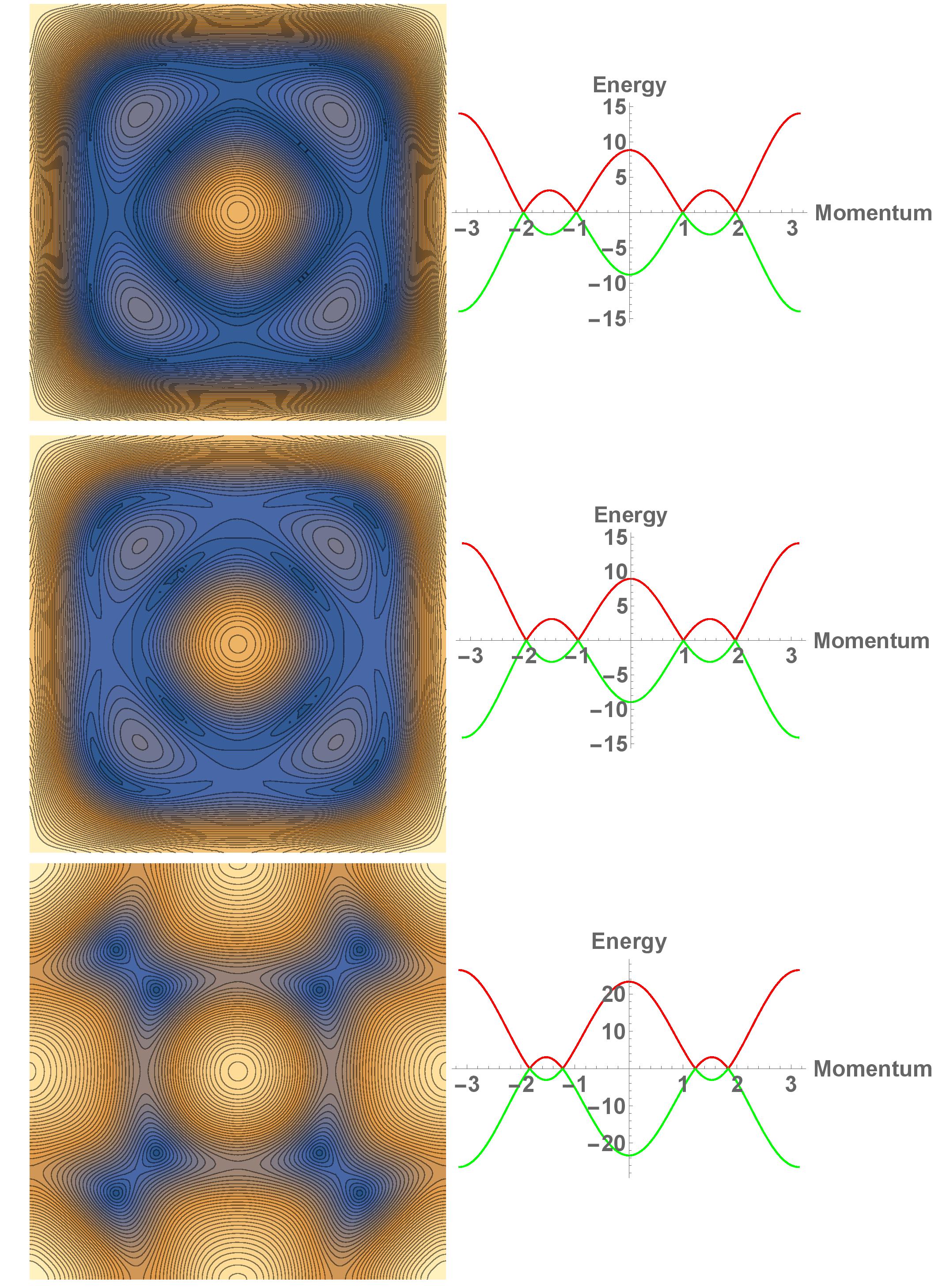
Figure 3: Particular realization of the Dirac Cones for $T_{1}=1$, $T_{2}=-3.9$, $T_{3}=1.8$, and $J/T_{1}=18$ (top), $27$ (middle), and $90$ (bottom panel). The superconducting paring was chosen to optimize the zero temperature Gibbs free energy $\Delta\sim 0.05,\,0.135,\,0.5$, respectively. The whole Brillouin zone from $(-\pi,-\pi)$ to $(\pi,\pi)$ is shown on the left and a cross section along the major diagonal on the right, which highlights $4$ of the Dirac cones.

To verify the existence and robustness of the Dirac cones predicted in the main text, we plot numerically the function $E_{+,-}\left(k\right)$ near the values of the hopping matrix elements $T_{1}=1$, $T_{2}=-3.9$, $T_{3}=1.8$, for various values of $J$ near the $\Delta$ that minimizes the free energy. We focus on the case of large $J/T_{1}=18,\,27,\,90$ (see Fig. 3), and we find eight cones in all cases, even though the exchange coupling is taken to be $\sim 5$ times larger then the relevant value for cuprate superconductors.

To get an estimate of the ratio of $J/T_{1}$ we note that for the cuprates $J\sim 0.13$ eV, the nearest neighbor hopping $t\sim 0.4$ eV key-36-1 (5, 3, 4), $t_{1}\simeq 0.35t$ key-30-2 (6), and in general $\left\langle b_{i_{1},\eta_{1}}^{\dagger}b_{i_{2},\eta_{2}}\right\rangle<\frac{1}{4}\left(1-p\right)$, as any boson bilinear must be less then the largest occupation number $\left\langle n_{i}\right\rangle=\frac{1}{4}\left(1-p\right)$. Recalling that $T_{1}=t_{1}\left\langle b_{i,\hat{x}}^{\dagger}b_{i+\hat{y},\hat{x}}\right\rangle$, we get for $p\simeq 0.2$ that $J/T_{1}\gtrsim 5$, likely of the order of $10-20$.

III Large N arbitrary S

The considerations given in the main text can be extended to multiple species ($N$) and different occupation number ($S$) of dimers. The meanfield studied in the main text becomes arbitrarily accurate in this limit. We consider the case of the square lattice but generalizations to different lattice geometries is straightforward. We consider $N$ different species of bosonic dimers $\gamma=1,2,...N$ living on the links of the lattice and $2N$ species of fermionic dimers $\sigma,\gamma=\uparrow 1;\uparrow 2;\ldots\uparrow N;\downarrow 1\;\ldots\downarrow N$ also living on the same links. We represent the dimers using $N$ species of bosons living on the links of the lattice $b_{i,\eta,\gamma}$ and $2N$ species of fermions $c_{i,\eta,\sigma,\gamma}$. The dimer Hilbert space can be mapped onto a subspace of the boson/fermion Hilbert space via the correspondence where $n_{i,\eta,\gamma}$ bosonic dimers of species $\gamma$ living on the link $i,i+\eta$ are identified with the state for the slave particles where the occupation number of the boson $\gamma$ on link $i,i+\eta$ is given by $n_{i,\eta,\gamma}$. Similarly for the fermions. Rather than enforcing the constraint of at most one dimer per link (which is redundant in the physical case where $N=S=1$), we introduce the constraint

$$\Pi_{i}^{N,S}\equiv\sum_{\gamma=1}^{N}\sum_{l\in v_{i}}n_{l,\gamma}+n_{l,\uparrow,\gamma}+n_{l,\downarrow,\gamma}-NS=0\,.$$ (17)

Here, for convenience of notation, $\ell\in v_{i}$ labels the four links $j,\eta$ that are attached to vertex $i$. In the dimer language this corresponds to the constraint that the total number of dimers of any species on all the links touching the vertex $i$ is given by $NS$. $S$ can be an arbitrary number and in the limit where $S$ becomes large the bosonic part of the dimer model becomes semiclassical. In the path integral formulation, the constraint can be written as

$$\Pi_{i}^{N,S}\sim\int d\lambda_{i}\exp\left[-\varepsilon\lambda_{i}\left(\sum_{\gamma=1}^{N}\sum_{l\in v_{i}}n_{l,\gamma}+n_{l,\uparrow,\gamma}+n_{l,\downarrow,\gamma}-NS\right)\right]\,,$$ (18)

where $\varepsilon$ is the length of a time slice.

There is no prescription to write a Hamiltonian for a large $N$ theory. However, in order to proceed further we need to write down Hamiltonians for our slave bosons/fermions that reduce to the Hamiltonian given in the main text in the case $N,S=1$ and are amenable to large $N$ expansion key-9 (7). All the Hamiltonians written in this section have a direct interpretation in terms of Hamiltonians for the dimers (they all correspond to various dimer hopping terms and terms that count the number of flippable dimer plaquettes). Note that it does not matter whether the Hamiltonians we produce respect the constraint in Eq. (17) as in the path integral formulation we insert projectors onto the physical space $\Pi_{i}^{N,S}$ at every time slice. The hint towards how to do this extension comes from the expressions derived around Eqs. (4) and (5) in the main text. Indeed in order to apply a HS transformation to our expressions we need to write our Hamiltonian (when restricted to a single plaquette) schematically in the form $H_{D}=AB$ where $A$ and $B$ are single particle operators for one species of dimer, either bosonic or fermionic (see the main text e.g. Eqs. (4), (5) and (6)). The main idea is to replace $H_{D}\rightarrow H_{D}^{NS}=\frac{1}{N}\sum_{\gamma_{1}=1}^{N}A_{\gamma_{1}}\sum_{\gamma_{2}=1}^{N}B_{\gamma_{2}}$. Here $A_{\gamma_{1}}$, $B_{\gamma_{2}}$ are single particle operators either bosonic or fermionic which are identical to $A$ and $B$ except they now carry an index $\gamma$. As such each HS transformation given in the main text corresponds to a different large $N$ Hamiltonian. In the large $N$ limit, with this extension, we present models where the HS mean-field becomes arbitrarily accurate. Qualitatively we expect mean-field theory to become more and more accurate as each particle interacts with $N$ particles with an interaction strength that is attenuated by $1/N$. We now proceed to give several examples of this procedure. We note that none of the Hamiltonians have any dependence on $S$. In particular we can replace

$$Vb_{i,\hat{x}}^{\dagger}b_{i,\hat{x}}b_{i+\hat{y},\hat{x}}^{\dagger}b_{i+\hat{y},\hat{x}}\rightarrow$$

$$\rightarrow\kappa_{1}\frac{V}{N}\left\{\sum_{\gamma_{1}}b_{i,\hat{x},\gamma_{1}}^{\dagger}b_{i,\hat{x},\gamma_{1}}\cdot\sum_{\gamma_{2}}b_{i+\hat{y},\hat{x},\gamma_{2}}^{\dagger}b_{i+\hat{y},\hat{x},\gamma_{2}}\right\}+\left(1-\kappa_{1}\right)\frac{V}{N}\left\{\sum_{\gamma_{1}}b_{i,\hat{x},\gamma_{1}}^{\dagger}b_{i+\hat{y},\hat{x},\gamma_{1}}^{\dagger}\cdot\sum_{\gamma_{2}}b_{i,\hat{x},\gamma_{2}}b_{i+\hat{y},\hat{x},\gamma_{2}}\right\}$$ (19)

where $\kappa_{1}$ is arbitrary and each value of $\kappa_{1}$ produces a different Hamiltonian. Similarly we have

$$Jb_{i,\hat{x}}^{\dagger}b_{i+\hat{y},\hat{x}}^{\dagger}b_{i,\hat{y}}b_{i+\hat{x},\hat{y}}+h.c\rightarrow$$

$$\rightarrow\kappa_{2}\frac{J}{N}\left\{\sum_{\gamma_{1}}b_{i,\hat{x},\gamma_{1}}^{\dagger}b_{i+\hat{y},\hat{x},\gamma_{1}}^{\dagger}\cdot\sum_{\gamma_{2}}b_{i,\hat{y},\gamma_{2}}b_{i+\hat{x},\hat{y},\gamma_{2}}+h.c.\right\}+\left(1-\kappa_{2}\right)\frac{J}{N}\left\{\sum_{\gamma_{1}}b_{i,\hat{x},\gamma_{1}}^{\dagger}b_{i,\hat{y}}\cdot\sum_{\gamma_{2}}b_{i+\hat{y},\hat{x},\gamma_{2}}^{\dagger}b_{i+\hat{x},\hat{y},\gamma_{2}}+h.c.\right\}$$ (20)

where again $\kappa_{2}$ is arbitrary. The Bose/Fermi part may be extended to the large $N$ limit in a similar manner. For instance

$$\sum_{\sigma}\sum_{i}\left\{-t_{1}b_{i,\hat{x}}^{\dagger}c_{i+\hat{y},\hat{x},\sigma}^{\dagger}c_{i,\hat{x},\sigma}b_{i+\hat{y},\hat{x}}+3\>terms\right.$$

$$-t_{2}b_{i+\hat{x},\hat{y}}^{\dagger}c_{i,\hat{y},\sigma}^{\dagger}c_{i,\hat{x},\sigma}b_{i+\hat{y},\hat{x}}+7\>terms$$

$$-t_{3}b_{i+\hat{x}+\hat{y},\hat{x}}^{\dagger}c_{i,\hat{y},\sigma}^{\dagger}c_{i+\hat{x}+\hat{y},\hat{x},\sigma}b_{i,\hat{y}}+7\>terms$$

$$\left.-t_{3}b_{i+2\hat{y},\hat{x}}^{\dagger}c_{i,\hat{y},\sigma}^{\dagger}c_{i+2\hat{y},\hat{x},\sigma}b_{i,\hat{y}}+7\>terms\right\}\rightarrow$$

$$\rightarrow\frac{1}{N}\sum_{\alpha}\sum_{i}\left\{-t_{1}\sum_{\gamma_{1}}c_{i+\hat{y},\hat{x},\alpha,\gamma_{1}}^{\dagger}c_{i,\hat{x},\alpha,\gamma_{1}}\cdot\sum_{\gamma_{2}}b_{i,\hat{x},\gamma_{2}}^{\dagger}b_{i+\hat{y},\hat{x},\gamma_{2}}+3\;terms\right.$$

$$-t_{2}\sum_{\gamma_{1}}c_{i,\hat{y},\alpha,\gamma_{1}}^{\dagger}c_{i,\hat{x},\alpha,\gamma_{1}}\cdot\sum_{\gamma_{2}}b_{i+\hat{x},\hat{y},\gamma_{2}}^{\dagger}b_{i+\hat{y},\hat{x},\gamma_{2}}+7\;terms$$

$$-t_{3}\sum_{\gamma_{1}}c_{i,\hat{y},\alpha,\gamma_{1}}^{\dagger}c_{i+\hat{x}+\hat{y},\hat{x},\alpha,\gamma_{1}}\sum_{\gamma_{2}}b_{i+\hat{x}+\hat{y},\hat{x},\gamma_{2}}^{\dagger}b_{i,\hat{y},\gamma_{2}}+7\;terms$$

$$\left.-t_{3}\sum_{\gamma_{1}}c_{i,\hat{y},\alpha,\gamma_{1}}^{\dagger}c_{i+2\hat{y},\hat{x},\alpha,\gamma_{1}}\sum_{\gamma_{2}}b_{i+2\hat{y},\hat{x},\gamma_{2}}^{\dagger}b_{i,\hat{y},\gamma_{2}}+7\;terms\right\}.$$ (21)

The four fermion term in the Hamiltonian (see Eq. (9)) is given by spin spin interactions and has a variety of large $N$ extensions which were previously tabulated key-11 (9, 10, 11, 8, 7). We will not repeat this procedure here. We note that, to produce superconductivity, the optimum extension is given by the $SP(2N)$ formalism key-11 (9, 10, 11). It is possible to do a HS decoupling on all these terms, based on the following identity

$$\exp\left(-\frac{\varepsilon}{N}\sum_{\gamma_{1}=1}^{N}A_{\gamma_{1}}\sum_{\gamma_{2}=1}^{N}B_{\gamma_{2}}\right)\sim\int dx_{1}\int dx_{2}\>\exp\left[\varepsilon N\left(x_{1}x_{2}-x_{1}\frac{1}{N}\sum_{\gamma_{2}}B_{\gamma_{2}}-x_{2}\frac{1}{N}\sum_{\gamma_{1}}A_{\gamma_{1}}\right)\right]\,.$$ (22)

The mean-field equations (stationary points of this integral) are given by $x_{2}=\frac{1}{N}\sum_{\gamma_{2}}\left\langle B_{\gamma_{2}}\right\rangle$ and $x_{1}=\frac{1}{N}\sum_{\gamma_{1}}\left\langle A_{\gamma_{1}}\right\rangle$. From this we see that the mean-field is simply a sum of $N$ copies of the mean-field for a single species problem and we can replace $x_{2}=\left\langle B\right\rangle$ and $x_{1}=\left\langle A\right\rangle$, where $A$ and $B$ are single particle operators. There is one saddle point which reduces to $N$ copies of the mean-field theories found in the main text.

In the limit where $N$ goes to infinity, the mean-field results become exact, see Ref. key-9, 7 (section 17.2). The derivation given in Ref. key-9, 7 works verbatim for our case. Indeed an integration over the bosonic and fermionic fields that appear in the partition function of our theory (for which the Hamiltonian is quadratic) may be performed to obtain:

$$Z=\int D\lambda_{i}D\left\{x_{i,j}\right\}\>\exp\left[N\left(\lambda_{i},\left\{x_{i,j}\right\}\right)\right]\,,$$ (23)

where $x_{i,j}$ are all the possible HS fields which we may introduce. The only dependence on $N$ is the overall scaling $\sim N$ of the action. Using an argument identical to Ref. key-9, 7 (section 17.2) it is possible to show that higher loop corrections to the partition function in Eq. (23) vanish as $\left(1/N\right)^{P-L}$, where $P$ is the number of propagators and $L$ is the number of loops. As such all the higher loop corrections vanish when $N\rightarrow\infty$, making mean-field exact.

IV Gauge symmetry

To discuss the various symmetries of our systems we focus for simplicity on the case when $N=1$ for arbitrary $S$ (this does not entail any additional complexity beyond the physical case of $S=1$). Consider the gauge transformation where we assign a $U\left(1\right)$ phase to each vertex of our system, namely where each boson and fermion operator $b_{i,\eta}$ and $c_{i,\eta,\sigma}$ on each link transforms as:

$$b_{i,\eta}\rightarrow e^{i\theta_{i}}b_{i,\eta}e^{i\theta_{i+\eta}},\quad c_{i,\eta,\sigma}\rightarrow e^{i\theta_{i}}c_{i,\eta,\sigma}e^{i\theta_{i+\eta}}\,.$$ (24)

Any Hamiltonian that preserves the constraint

$$\Pi_{i}^{S}\equiv\sum_{i,\eta\in i}n_{i,\eta}+n_{i,\eta,\uparrow}+n_{i,\eta,\downarrow}-S=0$$ (25)

is automatically invariant under the $U\left(1\right)$ Gauge transformation in Eq. (24). Indeed any Hamiltonian that preserves the constraint in Eq. (25) can be written as a sum of monomials each of which is a product of creation and annihilation operators. In order to preserve the constraint Eq. (25) we mush have the same number of creation and annihilation operators for the bosons/fermions at every vertex (otherwise the constraint is no longer satisfied). Under this condition, the total phase from phase factors in Eq. (24) associated with each vertex vanishes, leading to an invariant Hamiltonian. In particular, one can explicitly check that the Hamiltonians in Eqs. (2) in the main text are invariant under the gauge transformation given in Eq. (24).

This gauge transformation is compatible with many of the HS transformations introduced in the main text. For instance the HS transformation associated with the decoupling of the bosons,

$$H_{MF} =V\left(\sum_{P}\left(x_{i2}n_{i+\hat{y},\hat{x}}+n_{i,\hat{x}}x_{i1}-x_{i1}x_{i2}\right)+\sum_{P}\left(x_{i3}n_{i,\hat{y}}+n_{i+\hat{x}}x_{i4}-x_{i3}x_{i4}\right)\right)$$

$$+t\sum_{i}\kappa\left(z_{i1}^{*}b_{i,\hat{y}}b_{i+\hat{x},\hat{y}}+b_{i,\hat{x}}^{\dagger}b_{i+\hat{y},\hat{x}}^{\dagger}z_{i2}-z_{i1}^{*}z_{i2}+h.c.\right)+\frac{t}{2}\sum_{i}\left(1-\kappa\right)\left(w_{i1}^{*}b_{i+\hat{y},\hat{x}}^{\dagger}b_{i,\hat{y}}+\right.$$

$$\left.+b_{i,\hat{x}}^{\dagger}b_{i+\hat{x},\hat{y}}w_{i2}-w_{i1}^{*}w_{i2}+h.c.\right)+\frac{t}{2}\sum_{i}\left(1-\kappa\right)\left(w_{i3}^{*}b_{i+\hat{y},\hat{x}}^{\dagger}b_{i+\hat{x},\hat{y}}+b_{i,\hat{x}}^{\dagger}b_{i,\hat{y}}w_{i4}-w_{i3}^{*}w_{i4}+h.c.\right)\,,$$ (26)

is gauge compatible (here $\kappa$ is an arbitrary constant). One simply has to transform the variables $z_{i,j}$ and $w_{i,j}$ in the opposite way as the gauge transformation for the bosons. Focusing on a single plaquette and labeling the lower left corner site as $i$ with the other sites $i+\hat{x}$, $i+\hat{y}$ and $i+\hat{x}+\hat{y}$, the gauge transformation for the HS bosons is given by:

$$x_{i,j} \rightarrow x_{i,j}$$

$$z_{i,j} \rightarrow\exp\left[i\left(\theta_{i}+\theta_{i+\hat{x}}+\theta_{i+\hat{y}}+\theta_{i+\hat{x}+\hat{y}}\right)\right]z_{i,j}$$

$$w_{i1/2} \rightarrow\exp\left[i\left(\theta_{i}-\theta_{i+\hat{x}+\hat{y}}\right)\right]w_{i1/2}$$

$$w_{i3/4} \rightarrow\exp\left[i\left(\theta_{i+\hat{x}}-\theta_{i+\hat{y}}\right)\right]w_{i3/4}\,.$$ (27)

Similar considerations can be made about the boson fermion and the fermion fermion part of the Hamiltonian in the main text (in particular the HS transformations in Eqs. (6) and (9) are completely gauge compatible).

From this it would appear that the solutions to our mean-field equations lead to a large degeneracy of mean-fields. Indeed it would seem that any gauge transformation of the mean-field solutions leads to a different solution with the same energy and as such a different ground state. However, this is not the case: there is only one state of the physical system that can be obtained from two different states that differ by a gauge transformation. More precisely, after we project onto the physical subspace via the projection operators $\Pi_{i}^{S}$, Eq. (25), two states that differ by a gauge transformation given in Eq. (24) project onto the same state up to an unobservable overall phase. To show this, without loss of generality, assume that under the gauge transformation in Eq. (24) the state with no bosons/fermions transforms into itself, $\left|0\right\rangle\rightarrow\left|0\right\rangle$. Now an arbitrary state may be written as a linear combination of terms of the form:

$$b_{i_{1},\eta_{1}}^{\dagger}\,b_{i_{2},\eta_{2}}^{\dagger}\dots\,b_{i_{n},\eta_{n}}^{\dagger}\>c_{j_{1},\eta_{1},\sigma_{1}}^{\dagger}\dots\,c_{j_{m},\eta_{m},\sigma_{m}}^{\dagger}\left|0\right\rangle\,.$$ (28)

After projection we may as well assume that there are exactly $S$ $b_{i,\eta}/c_{i,\eta,\sigma}$’s at every vertex $i$ in the expression in Eq. (28). Under a gauge transformation,

$$b_{i_{1},\eta_{1}}^{\dagger}\dots\,b_{i_{n},\eta_{n}}^{\dagger}c_{j_{1},\eta_{1},\sigma_{1}}^{\dagger}\dots\,c_{j_{m},\eta_{m},\sigma_{m}}^{\dagger}\left|0\right\rangle\rightarrow$$

$$\!\!\!\!\!\rightarrow e^{-i\theta_{i_{1}}}\,b_{i_{1},\eta_{1}}^{\dagger}\,e^{-i\theta_{i_{1}+\eta_{1}}}\dots\;e^{-i\theta_{i_{n}}}\,b_{i_{n},\eta_{n}}^{\dagger}\,e^{-i\theta_{i_{n}+\eta_{n}}}\>e^{-i\theta_{j_{1}}}\,c_{j_{1},\eta_{1},\sigma_{1}}^{\dagger}\,e^{-i\theta_{j_{1}+\eta_{1}}}\dots\>e^{-i\theta_{j_{m}}}\,c_{j_{m},\eta_{m},\sigma_{m}}^{\dagger}\,e^{-i\theta_{j_{m}+\eta_{m}}}\left|0\right\rangle\,.$$ (29)

We can group the phases associated with every vertex together and, because of the constraint that there are exactly $S$ bosons/fermions at any vertex, this gauge transformation becomes a state independent phase:

$$\left|\Psi\right\rangle\rightarrow\exp\left(-iS\sum_{i}\theta_{i}\right)\left|\Psi\right\rangle\,.$$ (30)

IV.1 The Invariant Gauge Group

Here we consider the Projective Symmetry Group (PSG) construction, again focusing on the case where $N=1$. The main idea behind the PSG (which was originally introduced for spin systems key-18 (12, 13, 14, 15, 16, 17)) is that in order for a mean-field state to be invariant under a symmetry transformation of the system (e.g., a translation or a rotation), the mean-field ansatz needs not remain invariant under the transformation but needs only be invariant following a gauge transformation of the form in Eq. (27) (which does not change the state of the systems as discussed previously). Using this observation we may define the PSG of a mean-field ansatz key-18 (12, 13, 14, 15, 16, 17) as the set of all lattice transformations followed by gauge transformations (as in Eq. (27)) which leave the mean-field ansatz invariant. An important subgroup of the PSG is the IGG (Invariant Gauge Group) which is the set of all gauge transformations in Eq. (27) that leave the mean field ansatz invariant. We will now proceed to calculate the IGG for various lattices.

We only focus on HS generated mean-fields of the form in Eq. (26) which are gauge transformation compatible via Eq. (27) and ignore all other mean-fields. It can be checked directly that the mean-fields obtained by considering the fermion fermion or fermion boson part of the Hamiltonian do not change the value of the IGG. We begin with bipartite lattices, with sublattices labeled by $A$ and $B$. The first constraint we obtain by the gauge transformation in Eq. (27) is that $x_{i,j}=x_{i,j}$, i.e., it is gauge invariant and therefore it gives no further restrictions on the form of the gauge transformations. The second constraint is that

$$w_{i1/2} =\exp\left[i\left(\theta_{i}-\theta_{i+\hat{x}+\hat{y}}\right)\right]w_{i1/2}$$

$$w_{i3/4} =\exp\left[i\left(\theta_{i+\hat{x}}-\theta_{i+\hat{y}}\right)\right]w_{i3/4}\,.$$ (31)

We assume that the terms $w_{i,j}$ are non-zero (otherwise the mean-field lattice loses connectivity and breaks up into one dimensional sublattices). In this case we have that $\exp\left(i\theta_{i}\right)=\exp\left(i\theta_{i+\hat{x}+\hat{y}}\right)\equiv\exp\left(i\theta_{A}\right)$ and $\exp\left(i\theta_{i+\hat{x}}\right)=\exp\left(i\theta_{i+\hat{y}}\right)=\exp\left(i\theta_{B}\right)$. Therefore the IGG for a bipartite lattice (assuming the terms $z_{i,j}$ are zero) is simply $U\left(1\right)\times U\left(1\right)$ where there are two different phases living on the two sublattices $A$ and $B$.

When the decoupling fields $z_{i,j}$ are non-zero, we have the constraint

$$\begin{array}[]{l}\exp\left[i\left(\theta_{i}+\theta_{i+\hat{x}}+\theta_{i+\hat{y}}+\theta_{i+\hat{x}+\hat{y}}\right)\right]=\\ =\exp\left[2i\left(\theta_{A}+\theta_{B}\right)\right]=1\;,\end{array}$$ (32)

so that $\exp\left(i\theta_{A}\right)=\pm\exp\left(-i\theta_{B}\right)$ and the IGG becomes $U\left(1\right)\times\mathbb{Z}_{2}$. Adding fermions does not change the $U\left(1\right)\times\mathbb{Z}_{2}$. One simply gets another copy of the same set of equations. Qualitatively this is because the HS fields transform in a way determined by the transformation properties of fermion or boson bilinears under Eq. (24). Since the bosons and fermions transform in the same away under Eq. (24), it does not add any new “information” (or constraints) to consider fermions.

If we consider non-bipartite lattices, the constraint $x_{i,j}=x_{i,j}$ again does not effect the IGG. On the contrary, the constraints in Eq. (31) insure that the phases $\theta_{i}$ and $\theta_{j}$ for any two sites that can be reached by a finite number of translations along lines joining second nearest neighbors along a plaquette is the same. Since any two sites on a non-bipartite lattice may be joined that way, the IGG when the $w_{ij}\neq 0$ is $U\left(1\right)$, i.e., the same phase for every site.

When the terms $z_{ij}$ do not vanish, we have that

$$\begin{array}[]{l}\exp\left[i\left(\theta_{i}+\theta_{i+\hat{x}}+\theta_{i+\hat{y}}+\theta_{i+\hat{x}+\hat{y}}\right)\right]=\exp\left(4i\theta\right)=1\;,\end{array}$$ (33)

which means that the IGG is now given by $\mathbb{Z}_{4}$. Adding fermions does not change the $\mathbb{Z}_{4}$, as once again we get multiple copies of the same equations. The PSG for the boson/fermion system may be computed directly. For example one can check that the Algebraic PSG for the dimer system is the same as the Algebraic PSG for a bosonic spin liquid on the same lattice with the same IGG key-18 (12, 13, 14, 15, 16, 17). Indeed the gauge degrees of freedom are identical and the “commutator” constraint equations key-18 (12, 13, 14, 15, 16, 17) are of the same form for the same lattice and the same IGG.

References

• (1) D. S. Rokhsar and S. A. Kivelson, Phys. Rev. Lett. 61, 2376 (1988).
• (2) A. Sen, K. Damle and T. Senthil Phys. Rev. B 76, 235107 (2007); D. Poilblanc, K. Penc, and N. Shannon Phys. Rev. B 75 220503 (2007); D. Poilblanc, Phys. Rev. B. 76, 115104 (2007).
• (3) A. F. Albuquerque, H. G. Katzgraber, M. Troyer and G. Blatter Phys. Rev. B 78, 014503 (2008).
• (4) R. Moessner and S. L. Sondhi, Phys. Rev. B 68, 054405 (2003).
• (5) R. Moessner, S. L. Sondhi and E. Fradkin, Phys. Rev. B 65, 024504 (2002).
• (6) F. Vernay, A. Ralko, F. Becca and F. Mila, Phys. Rev. B 74, 054402 (2006).
• (7) H. P. Buchler, M. Hermele, S. D. Huber, M. P. A. Fisher and P. Zoller, Phys. Rev. Lett. 95, 040402 (2005).
• (8) E. Fradkin, D. A. Huse, R. Moessner, V. Ognasian and S. L. Sondhi, Phys. Rev. B 69, 224415 (2004); A. Vishwanath, L. Balents and T. Senthil, Phys. Rev. B 69, 224415 (2004).
• (9) X. G. Wen, Quantum field theory of many-body systems, (Oxford University press, Oxford 2004).
• (10) M. Punk, A. Allais and S. Sachdev, PNAS 112, 9552 (2015).
• (11) D. Chowdhury and S. Sachdev The enigma of the pseudogap phase in the cuprate superconductors in Quantum criticality in condensed matter: phenomena, materials and ideas in theory and experiment J. Jedrzejewski eds. (Word scientific publishing co, Singapore 2016).
• (12) A. A. Patel, D. Chowdhury, A. Allais, and S. Sachdev, arXiv 1602.05954.
• (13) Y. Ando, Y. Kurita, S. Komiya, S. Ono, and K. Segawa, Phys. Rev. Lett. 92, 197001 (2004).
• (14) J. Orenstein, G. A. Thomas, A. J. Millis, S. L. Cooper, D. H. Rapkine, T. Timusk, L. F. Schneemeyer, and J. V. Waszczak, Phys. Rev. B 42, 6342 (1990).
• (15) S. Uchida, T. Ido, H. Takagi, T. Arima, Y. Tokura, and S. Tajima, Phys. Rev. B 43, 7942 (1991).
• (16) P. A. Lee, N. Nagaosa and X. G. Wen, Rev. Mod. Phys. 78 (2006).
• (17) A. Damascelli, Z. Hussain, and Z.-X. Shen, Rev. Mod. Phys. 75, 473 (2003).
• (18) K. M. Shen, F. Ronning, D. H. Lu, F. Baumberger, N. J. C. Ingle, W. S. Lee, W. Meevasana, Y. Kohsaka, M. Azuma, M. Takano, H. Takagi, and Z.-X. Shen, Science 307, 901 (2005).
• (19) H.-B. Yang, J. D. Rameau, Z.-H. Pan, G. D. Gu, P. D. Johnson, H. Claus, D. G. Hinks, and T. E. Kidd, Phys. Rev. Lett. 107, 047003 (2011).
• (20) J. Gonsalez, M. A. Martin-Delgado, G. Sierra, A. H. Vozmediano, Quantum electron liquids and high-Tc superconductivity (Springer, Berlin 1995).
• (21) J. Klamut, B. W. Veal, B. M. Dabrowski, P. W. Klamut, M. Kazimerski eds. Recent developments in high temperature superconductivity (Springer Verlag, Berlin 1995).
• (22) At first glance it appears that there are more gauge transformations that preserve the Hamiltonian. In particular it looks like the transformation $b_{i,\eta}\rightarrow e^{i\theta_{i,\eta}}b_{i,\eta}$ and $c_{i,\eta,\sigma}\rightarrow e^{i\theta_{i,\eta}}c_{i,\eta,\sigma}$, subject to the constraint that the phases around a plaquette add up to a multiple of $2\pi$ $\theta_{i,\hat{x}}-\theta_{i+\hat{x},\hat{y}}+\theta_{i+\hat{y},\hat{x}}-\theta_{i,\hat{y}}=2\pi n$, is another set of gauge transformations. Here $n$ is an integer and $i,\hat{x}$, $i+\hat{x},\hat{y}$, $i+\hat{y},\hat{x}$ and $i,\hat{y}$ are four links arranged counter clockwise around a plaquette. However one can verify (by explicitly constructing the gauge transformations) that every gauge transformation of this form can be written as a gauge transformation of the form in Eq. (3).
• (23) See supplementary online information.
• (24) S. S. Lee, Phys. Rev. B 78, 085129 (2008)
• (25) M. Hermele, T. Senthil, M. P. A. Fisher, P. A. Lee, N. Nagaosa, and X. G. Wen, Phys. Rev. B 70, 214437 (2004).
• (26) K.-S. Kim, Phys. Rev. B 72, 245106 (2005).
• (27) M. Ogata, and H. Fukuyama, Rep. Prog. Phys. 71, 036501 (2008).
• (28) K. S. Raman, R. Moessner and S. L. Sondhi, Phys. Rev. B 72, 064413 (2005).

References

• (1) D. S. Rokhsar and S. A. Kivelson, Phys. Rev. Lett. 61, 2376 (1988).
• (2) K. S. Raman, R. Moessner and S. L. Sondhi, Phys. Rev. B 72, 064413 (2005).
• (3) J. Gonsalez, M. A. Martin-Delgado, G. Sierra, A. H. Vozmediano, Quantum electron liquids and high-Tc superconductivity (Springer, Berlin 1995).
• (4) J. Klamut, B. W. Veal, B. M. Dabrowski, P. W. Klamut, M. Kazimerski eds. Recent developments in high temperature superconductivity (Springer Verlag, Berlin 1995).
• (5) M. Ogata, and H. Fukuyama, Rep. Prog. Phys. 71, 036501 (2008).
• (6) M. Punk, A. Allais and S. Sachdev, PNAS 112, 9552 (2015).
• (7) A. Auerbach, Interacting electrons and quantum magnetism (Springer Verlag, New York 1994).
• (8) D. P. Arovas and A. Auerbach, Phys. Rev. B 38, 316 (1988).
• (9) N. Read and S. Sachdev, Phys. Rev. Lett. 66, 1773 (1991).
• (10) S. Sachdev and N. Read, Int. J. Mod Phys. B 5, 219 (1991).
• (11) S. Sachdev, Phys. Rev B 45, 12377 (1992).
• (12) X. G. Wen, Phys. Rev. B 65, 165113 (2002).
• (13) T. P. Choy and Y. B. Kim, Phys. Rev. B 80, 064404 (2009).
• (14) S. Bieri, C. Lhullier, and L. Messio, arXiv 1512.00324
• (15) X. Yang and F. Wang, arXiv 1507.07621
• (16) Y.-M. Lu and Y. Ran, arXiv 1005.4229
• (17) F. Wang and A. Vishwanath, Phys. Rev. B 74, 174423 (2006).