Master, Chan, and Bambos

Myopic Scheduling of Jobs with Decaying Value

Myopic Policies for Non-Preemptive Scheduling of Jobs with Decaying Value

Neal Master Department of Electrical Engineering, Stanford University, nmaster@stanford.edu Carri W. Chan Decision, Risk, and Operations, Columbia Business School, cwchan@columbia.edu Nicholas Bambos Department of Management Sciences & Engineering and Department of Electrical Engineering, Stanford University, bambos@stanford.edu

In many scheduling applications, minimizing delays is of high importance. One adverse effect of such delays is that the reward for completion of a job may decay over time. Indeed in healthcare settings, delays in access to care can result in worse outcomes, such as an increase in mortality risk. Motivated by managing hospital operations in disaster scenarios, as well as other applications in perishable inventory control and information services, we consider non-preemptive scheduling of jobs whose internal value decays over time. Because solving for the optimal scheduling policy is computationally intractable, we focus our attention on the performance of three intuitive heuristics: (1) a policy which maximizes the expected immediate reward, (2) a policy which maximizes the expected immediate reward rate, and (3) a policy which prioritizes jobs with imminent deadlines. We provide performance guarantees for all three policies and show that many of these performance bounds are tight. In addition, we provide numerical experiments and simulations to compare how the policies perform in a variety of scenarios. Our theoretical and numerical results allow us to establish rules-of-thumb for applying these heuristics in a variety of situations, including patient scheduling scenarios.

1 Introduction

Managing delays in queueing networks has been the focus of a large body of work (e.g. Mandelbaum and Stolyar (2004), Dewan and Mendelson (1990), and Van Mieghem (2003) among many others). Typically, the undesirability of and dissatisfaction due to incurred delays serve as the primary motivation for minimizing delays. However, there are other adverse effects of delays, which often are not accounted for. For instance, in healthcare settings, delays in access to care can result in deterioration of a patient’s health state, thereby reducing the efficacy of the resulting care. In this work, we consider how to prioritize jobs (e.g. patients) when the reward for completing any particular job decreases over time.

Delays in healthcare are rampant. A study by Poon et al. (2004) indicates that over 60% of physicians reported dissatisfaction in the timeliness of test results, which can create treatment delays and, ultimately, lead to increased patient mortality and increased healthcare costs. Indeed, in the case of intensive care, delays in treatment often lead to deterioration of patient health and this can eventually reduce the efficacy of various treatments (McQuillan et al. 1998). This also occurs for cardiac arrest (Chan et al. 2008, Buist et al. 2002), angioplasty for acute myocardial infarctions (Luca et al. 2004), and is particularly true for children (Sharek et al. 2007). In this work, we capture the impact of delayed treatment on mortality risk and other health outcomes by allowing for the reward for completing a job to decay arbitrarily. In contrast to our work here, recent work by Chan et al. (2015) examines the impact of delayed treatment on service time.

For a specific scenario in healthcare where scheduling of jobs with decaying values is of interest, we start by considering patient triage in the aftermath of mass casualty incidents. In these situations, medical resources are overwhelmed by a sharp increase in demand. In both civilian and military situations, medical personnel, operating rooms, and ambulances need to be judiciously allocated so as to minimize the number of deaths and permanent injuries. Treatment delays will reduce survivial probabilities so rapid scheduling is a necessity. Triage practices have evolved over time, but must continue to advance as new disasters and new technologies can render previous strategies obsolete (Iserson and Moskop 2007, Moskop and Iserson 2007). There has been recent work examining patient triage in disaster scenarios by the operations management community (e.g. Argon et al. (2008, 2011), Chan et al. (2013)); yet, none have considered an arbitrary decay in reward as we do here.

While the primary motivation for our work is patient triage in mass casualty events, we note that the reward decay dynamics we consider in this work extend to other applications as well. For example, in food processing, perishable food items decay in market value as their expiration dates approach and efficient scheduling is necessary to maximize profits. Managers must account for variations in customer orders, equipment availability, raw materials, deliveries, processing rates, and food freshness when making decisions regarding the production of perishable foods like ice cream and yogurt (Jakeman 1994). As another example, scheduling jobs with deadlines has been of particular interest in information services and computing. In this case, the value of a job decays according to a step function. For example, deadlines are useful for ensuring high level of quality for customers who are streaming multimedia (Dua and Bambos 2007, Dua et al. 2010). Deadlines have also been considered in more general “data broadcast” problems which lead to a number of combinatorial optimization problems (Kim and Chwa 2004, Zheng et al. 2006).

Though the aforementioned applications are quite varied, they share a number of key similarities. In each case, we need to dynamically schedule jobs with decaying value for processing/service. The value of the jobs decays over time and we seek to capture as much of this value as possible. Motivated primarily by patient scheduling in disaster scenarios, we choose to focus on non-preemptive scheduling of a “clearing system” in which all jobs are present at the initial time (see Argon et al. (2011) and the references therein). To the best of our knowledge, we are the first to account for the fact that jobs each have an internal value which may decay over time. For each job, the function which governs this decay is deterministic and non-increasing; however, the manner of this decay is permitted to be arbitrary.

The arbitrary decay generalizes the idea of having jobs with deadlines which is a common modeling construct (e.g. Argon et al. (2008), Chan et al. (2013), Dua and Bambos (2007), Kim and Chwa (2004)). When jobs have deadlines, this corresponds to step-wise value decay: the internal value of the job will abruptly transition from full value to zero value after the deadline. This sharp transition can be thought of as a “hard” deadline. In constrast, our model allows for “soft” deadlines. That is, rather than having the internal value of a job abruptly decay from full value to zero value, the decay functions in our paper allow for the internal value of a job to gradually decay from full value to zero value. The time at which the job reaches zero value can still be thought of as a deadline, but because the transition from full value to zero value is gradual, the deadline is “soft” rather than “hard.” The arbitrary decay associated with soft deadlines allows for additional modeling flexibility beyond what is allowed by hard deadlines. Our model allows for both soft and hard deadlines as well as heterogeneity amongst the jobs in the system, thus offering a substantial generalization over previously studied scheduling models. Soft deadlines have recently been considered in some service rate control problems (e.g. Master and Bambos (2014, 2015)) but not in scheduling problems.

This modeling generalization is particularly important in patient scheduling applications. In the patient scheduling literature (e.g. Argon et al. (2008), Chan et al. (2013)), hard deadlines are used to model the time of mortality due to the injury/ailment at hand. However, this may not capture all of the nuances associated with the patient health in disaster scenarios, and soft deadlines may be more appropriate. For example, consider the patient triage scheme developed by Sacco et al. (2005). By consulting a group of physicians, Sacco et al. design a “health score” which they call RPM (Respiratory rate, Pulse rate, and Motor response) which decays over 30 minute time intervals. In Figure 1 we have plotted a few of the decaying RPM curves from (Sacco et al. 2005, Table 5). Note that the decay is sometimes linear but not necessarily. This motivates the arbitrary decay in our model. We emphasize that while Sacco et al. prioritize patients based on their gradually decaying health, they do so in a static manner and do not allow for dynamic patient scheduling. A key feature of our model is that we incorporate decaying job value and dynamic non-preemptive scheduling. We will discuss Sacco et al. (2005) more in the literature review.

Example RPM (Respiratory rate, Pulse rate, and Motor response) curves from Table 5 of Sacco et al. (2005). The RPM scores provide a metric for patient health decay. The scores take integer values $\left\{0,1,\ldots,12\right\}$ and decay over 30 minute time increments.

While soft and hard deadlines are useful modeling techniques (particularly for patient scheduling applications), we will show that maximizing the total value over time is computationally intractable. As such, we turn our attention to a number of intuitive, yet sub-optimal scheduling heuristics. In doing so, we wish to examine how well one can expect heuristics which do not account for future system dynamics to perform. Additionally, we aim to identify which heuristics are most effective for various different situations. More specifically, we consider three different heuristics:

1. Whenever there is a free server, the greedy policy schedules the job which maximizes the expected reward generated by the completion of that job, where the expectation is taken with respect to the job’s service time distribution. As such, the reward considered by this heuristic accounts for the decay in value of the job.

2. Whenever there is a free server, the rate greedy policy schedules the job with the maximum expected reward rate. This simply takes the expected reward generated by the completion of the job as considered by the greedy policy and divides it by the expected service time of the job in order to estimate the reward generated per unit of time during the processing of the scheduled job.

3. Whenever there is a free server, the Earliest Deadline First (EDF) policy, schedules the job whose value decays to 0 soonest. In order for this policy to be well defined, we must assume that for each job there is a finite time at which the value generated for completing the job is equal to 0, i.e. each job has a final deadline. The EDF policy schedules jobs whose deadlines are most imminent and have not yet passed.

We provide performance guarantees for each heuristic and are able to show that in some situations, these bounds are tight. We further explore the performance across the heuristic policies through simulation and provide some rules-of-thumb for when each of the policies is most appropriate. In particular, our simulations support the following rules:

• The rate greedy policy is the most robust heuristic in that it seems to always performs well and that for large numbers of jobs with high levels of heterogeneity, it will perform better than the other two heuristics.

• The greedy policy is also a very good heuristic. For many small scale problems, it can outperform the other heuristics. While the rate greedy policy generates more reward for large problems, the performance of the greedy policy is not far behind.

• EDF can outperform the greedy policies, but it is not very robust. We identify a few scenarios in which the performance of EDF is on par with the two greedy policies, but we note that slight deviations from these scenarios will lead to poor performance for EDF.

The remainder of the paper is outlined as follows. We conclude this section with a brief overview of some related literature. In Section 2 we introduce our model and the scheduling problem we consider. We show that while the problem is well-posed, it is computationally intractable. As such, we turn to heuristic policies in Section 3. We provide performance guarantees for three different heuristics and briefly discuss how the proofs can be leveraged to provide performance guarantees for other myopic policies. In addition to the general performance guarantees, we show that there are situations in which each policy is better than the other two. We explore this more in Section 4 via numerical examples. We use these results to extract rules-of-thumb for understanding when each heuristic should (or should not) be used. We conclude in Section 5. Proofs of our mathematical results are given in the appendix.

1.1 Literature Review

Our work is related to the healthcare operations management literature on patient triage and scheduling. While our primary motivation is scheduling patients in mass casualty events, our model also has some similarities to work done in perishable inventory control and information services. More generally, our work is related to theoretical work in scheduling and the evaluation of heuristic policies.

In the healthcare operations management literature, clearing models for jobs with value decay have been used to study triage and patient scheduling in mass casualty incidents. Argon et al. (2008) consider a clearing system where jobs are characterized by random service times as well as random deadlines. They show that if the jobs can be ordered in a particular way such that the job with the shortest deadline also has the shortest service time, then an optimal policy is to give priority to the most “time-critical” job. Unfortunately, jobs do not always exhibit this ordering and, in general, the time-critical first (TCF) heuristic performs poorly. Our model of job decay is quite different as we allow for arbitrary, deterministic, non-increasing functions rather than binary functions which are stochastic. We demonstrate that like the TCF policy, the EDF policy also performs poorly in general, but it can also do well in certain special cases. Moreover, we also consider the performance of other policies and provide performance guarantees for them.

In related work, Mills et al. (2013) consider a fluid model for patient triage which considers dynamic patient survival probabilities. Their model focuses on a finite number of patient classes each with time varying rewards for service completion. By controlling the service rates for each class, they seek to maximize the long-term reward. We also consider dynamic patient scheduling. However, instead of using fluid models, which necessarily only capture “average” behavior (see Gamarnik (2010) for a survey), we consider a stochastic model and evaluate the performance of a number of heuristics. Additionally, while Mills et al. focus on ambulance transportation, we have calibrated our simulations to provide insight into scheduling surgical procedures in mass casualty events (see Section 4.2).

Similar to our model, Sacco et al. (2005) consider how to do mass casualty triage given patients have a “health score” which decays over time. This score decreases in a deterministic fashion over the finite time horizon and maps to a survival probability. The deterministic health score system is determined by the Delphi method, an iterative survey technique which is often used to aggregate expert opinions in a quantitative manner (see Linstone et al. (1975) for an overview of the Delphi method). This suggests that precise formulae for the deterministic value decay in our model could be determined in a similar fashion. Given various capacity constraints, a linear program is solved to decide how many patients of each score should be scheduled in each time slot so as to maximize the expected number of survivors. Note that this linear program is solved once at the beginning of the time horizon. As a result, while this technique does allow for arbitrary patient health decay, it does not allow for dynamic scheduling decisions. In contrast, the policies we consider, albeit myopic, are dynamic and can adapt to a changing environment.

Another line of research in patient scheduling has been to rely on sophisticated computational techniques to approximately compute optimal policies. For example, Patrick et al. (2008) pose a patient scheduling problem as a Markov Decision Problem (MDP) and use linear programming based Approximate Dynamic Programming (ADP) techniques to find high performance policies. We also leverage the theory of MDPs for studying our scheduling model. However, rather than focus on computational techniques, we investigate the efficacy of simple heuristics which are easy to implement.

While our primary motivation is healthcare operations, we note that our model also captures some features present in other types of systems. In inventory control, Federgruen and Wang (2015) recently showed that “shelf-age-dependent” and “delay-dependent” cost structures are equivalent to traditional “level dependent” cost structures. These time-varying costs are conceptually similar to the value decay functions which we employ, but their focus is on inventory models rather than patient scheduling systems. As another example, we note that jobs with deadlines have played an important role in the information technology literature. For example, Dua and Bambos (2007) consider the problem of scheduling multiple traffic streams over a wireless downlink. Their solution can be thought of as an algorithmic incarnation of our rate greedy heuristic which accounts for time-varying parameters and user preferences. Our work expands on these ideas significantly by considering more general value decay functions and providing performance guarantees.

In the healthcare context, it is typical to consider non-preemptive scheduling and specifically in mass casualty incidents, it is typical to consider clearing systems (see Argon et al. (2011) and the references therein). The key idea is that after a disaster, the victims will undergo triage in one large batch and once a patient is undergoing a procedure it is unsafe to preempt service. If the scheduling were preemptive, then we could apply the theory of stochastic depletion problems (Chan and Farias 2009). However, because the scheduling discipline is non-preemptive, when a server begins work on a job, it will continue until the job is complete. In this sense, scheduling decisions tend to have a greater impact on the future evolution of the system and intuitively, this makes non-preemptive scheduling a more difficult problem. In particular, we will later see that computing an optimal non-preemptive scheduling policy for our system is at least as difficult as solving a broad class of NP-hard combinatorial optimization problems.

In the more traditional case where the value of each job does not decay over time and there is a single server, job scheduling problems are often cast in the framework of multi-armed bandit problems in which the Gittens Index Theorem allows for efficient computation of optimal solutions (see Gittins et al. (2011) and the references therein). When the internal state of each job evolves over time, we are faced with a restless bandit problem (Whittle 1988). Index policies for restless bandit problems have been shown to be asymptotically optimal (for large numbers of jobs) in the case that the ratio between of the number of jobs and servers is constant and a certain differential equation describing a fluid approximation of the system is globally stable (Weber and Weiss 1990). However, verifying the stability of this differential equation is not always straightforward. In addition, the indices in this result come from the Lagrange multipliers of an associated optimization problem and as a result, this type of policy may not be easy to implement in applications.

Still, there exists special cases where restless bandit problems admit solutions which are easy to compute and implement. In a Markovian setting where the reward for serving a user decays exponentially as a function of the user’s sojourn time, a greedy policy which seeks to maximize immediate expected rewards is an optimal policy (Dalal and Jordan 2005). This type of greedy policy can also be framed as a $c\mu$-type policy (see Walrand (1988) for a review of such policies). The $c\mu$-type policy is shown to be optimal in a heavy traffic setting (Mandelbaum and Stolyar 2004). These results partially motivate the work in this paper. We consider similar greedy policies but with arbitrary job value decay. In this more general setting, the greedy policies are not optimal and so we turn out attention to establishing bounds on their sub-optimality.

2 Model Formulation

We now formally introduce our model and discuss the optimization of the scheduling problem we consider here. While we are primarily motivated by patient triage in mass casualty events, we present a general model and connect back to the healthcare setting using simulation in Section 4.2.

2.1 System Dynamics and Dynamic Programming Formulation

We consider a set of $J$ jobs indexed by $j\in\mathcal{J}=\left\{1,2,\ldots,J\right\}$. Job $j\in\mathcal{J}$ has a random service time $\sigma_{j}$ taking values in $\left\{1,2,3,\ldots\right\}$. Let the distribution of $\sigma_{j}$ be $F_{j}(\cdot)$. The processing times are statistically independent and each has a finite mean. There are $N$ identical processors/servers indexed by $n\in\mathcal{N}=\left\{1,2,\ldots,N\right\}$. Each processor has unit service rate and can process a single job at a time. Service is non-preemptive in the sense that once a processor begins work on a job, the processor will continue to work on this job until the job is completed. Time is slotted and indexed by $t\in\left\{0,1,2,\ldots\right\}$.

Let $B_{j}(t)$ be the residual service time of job $j$ at time $t$ and let $B(t)=(B_{1}(t),\ldots,B_{J}(t))$ be the total system backlog. We know that $B(0)=(\sigma_{1},\ldots,\sigma_{J})$ and if all jobs have completed at time $T$, $B(T)=(0,\ldots,0)$. Each job service time is random and the realization can only be seen after the job has completed processing. Therefore, to make optimal scheduling decisions, we must track the observable backlog vector denoted by $b(\cdot)$:

$$\begin{split}b_{j}(t)=\left\{\begin{array}[]{cl}\bot,&\mbox{job $j$ hasn't begun processing}\\ t^{\prime},&\mbox{job $j$ began processing at time $t^{\prime}<t$ and is still being processed}\\ \top,&\mbox{job $j$ has completed processing}\end{array}\right.\end{split}$$ (1)

Because the service time distributions are known, $b(t)$ encodes the information necessary to determine the distribution of $B(t)$. We next define the state $p_{n}(t)$ of processor $n\in\mathcal{N}$ as follows:

$$p_{n}(t)=\left\{\begin{array}[]{ll}j,&\mbox{if processor $n$ is executing job $j\in\cal J$ at the beginning of time slot $t$}\\ 0,&\mbox{if processor $n$ is free at the beginning of time slot $t$}\end{array}\right.$$ (2)

The processor state vector is then defined as $p(t)=(p_{1}(t),\ldots,p_{N}(t))$. With these definitions, we can take the system state at time $t$ as

$$s_{t}=(b(t),p(t))$$ (3)

where we will sometimes simply write $s$ when the dependence on $t$ is understood. We denote the state space

$$\mathcal{S}\subseteq(\left\{\bot\right\}\cup\mathbb{N}\cup\left\{\top\right\})^{J}\times\left\{0,1,\ldots,J\right\}^{N}.$$ (4)

Note that at the beginning of each time slot, we can schedule job $j$ on processor $n$ if and only if $b_{j}(t)=\bot$ and $p_{n}(t)=0$.

Given state $s$, let $\mathcal{A}(s)$ be the set of feasible scheduling actions. A scheduling action is a set of pairings between jobs and processors so if $A\in\mathcal{A}(s)$, then $(j,n)\in A$ only if $b_{j}(t)=\bot$ and $p_{n}(t)=0$. In addition, since each processor can only work on a single job at a time, if $(j,n)\in A$ and $(j^{\prime},n^{\prime})\in A$ then $j\neq j^{\prime}$ and $n\neq n^{\prime}$. If the system is in state $s$ at time $t$ and action $A$ is take, let $S^{+}(s,A)$ be the random state at time $t+1$.

If job $j$ is completed at the end of time slot $t$, we garner a non-negative reward $v_{j}(t)$. We assume $v_{j}(\cdot)\geq 0$ and that $v_{j}(\cdot)$ is non-increasing. Therefore, $v_{j}(\cdot)$ defines the deterministic time-varying value of job $j$. For example, if job $j$ has a value $\nu_{j}$ and a deterministic deadline $d_{j}$, then we can take $v_{j}(t)=\nu_{j}\mathbf{1}_{\left\{t\leq d_{j}\right\}}$.

Recall that if job $j$ is scheduled on processor $n$ at the beginning of time slot $t$, it will complete processing at the end of time slot $t+\sigma_{j}$. Therefore, if the scheduler chooses action $A\in\mathcal{A}(s)$, the resulting reward will be

$$R_{t}(s,A)=\sum_{(j,n)\in A}v_{j}(t+\sigma_{j}).$$ (5)

We restrict our attention to deterministic policies $\pi\in\Pi$ such that if $s\in\mathcal{S}$, then $s\mapsto\pi_{t}(s)\in\mathcal{A}(s)$. We can now define the value function of policy $\pi$ as

$$V_{t}^{\pi}(s)=\mathbb{E}\left[\left.\sum_{\tau=t}^{\infty}R_{\tau}(s_{\tau},\pi_{\tau}(s_{\tau}))\right|s_{t}=s\right].$$ (6)

The optimal value function is then defined as

$$V_{t}^{*}(s)=\max_{\pi\in\Pi}V_{t}^{\pi}(s).$$ (7)

Any optimal policy which achieves this supremum is denoted $\pi^{*}$.

2.2 Preliminary Mathematical Results

Our problem formulation lends itself to an MDP approach. Given the recursive optimality equations (i.e. the Bellman equation) associated with an MDP, one can compute the optimal value function and find an optimal policy via standard techniques (value iteration, policy iteration, and linear programming (Bertsekas 2012)). Our first theorem characterizes the value function in terms of a Bellman equation, thus demonstrating that this is (in principle) a valid approach to the problem.

Theorem 2.1

The quantities in (6) and (7) are well-defined. An optimal policy $\pi^{*}$ exists and is characterized by the following Bellman equation:

$$V_{t}^{*}(s)=\max_{A\in\mathcal{A}(s)}\left\{\mathbb{E}[R_{t}(s,A)]+\mathbb{E}[V_{t+1}^{*}(S^{+}(s,A))]\right\}.$$ (8)

Our next theorem shows that this approach is not computationally tractable. Dynamic programming problems with large state and action spaces typically suffer from the curse of dimensionality. However, our particular problem is possibly even more difficult to solve. As mentioned before, requiring non-preemptive scheduling adds a combinatorial “twist” to the problem. A broad class of “knapsack” problems (see Martello and Toth (1990)) can be reduced to our problem and as a result, our general scheduling problem is NP-hard (see Cormen et al. (2009) for an introduction to complexity theory and NP-hardness).

Theorem 2.2

Computing $\pi^{*}$ is NP-hard.

3 Heuristic Policies and Performance Guarantees

We have just seen that while the non-preemptive scheduling problem can be solved in principle, it is unlikely that there is a computationally tractable way of doing so. As such, we turn our attention to heuristics which are intuitive and easy to use in practice. Unlike the optimal policy, which solves (8), the heuristics we consider ignore the impact of the scheduling decision on the future value. We focus on these particular heuristics because they have been studied in other contexts (e.g. Dua et al. (2010), Dalal and Jordan (2005), Mandelbaum and Stolyar (2004)) but we will briefly comment on how our proofs can be extended to other policies. The heuristics are defined as follows:

1. A greedy policy selects the jobs with the largest expected reward:

   $$\pi_{t}^{G}(s)\in\argmax_{A\in\mathcal{A}(s)}\left\{\mathbb{E}[R_{t}(s,A)]\right\}=\argmax_{A\in\mathcal{A}(s)}\left\{\sum_{(j,n)\in A}\mathbb{E}[v_{j}(t+\sigma_{j})]\right\}$$

2. A rate greedy policy selects the jobs with the largest expected reward rate:

   $$\pi_{t}^{g}(s)\in\argmax_{A\in\mathcal{A}(s)}\left\{\sum_{(j,n)\in A}\frac{\mathbb{E}[v_{j}(t+\sigma_{j})]}{\mathbb{E}[\sigma_{j}]}\right\}$$

3. An Earliest Deadline First (EDF) policy schedules the jobs with the most imminent deadline:

   $$\pi_{t}^{EDF}(s)\in\argmin_{A\in\mathcal{A}(s)}\left\{\sum_{(j,n)\in A}\frac{d_{j}-t}{\mathbf{1}_{\left\{d_{j}\geq t\right\}}}\right\}$$

   where $d_{j}=\arg\sup_{t}\{v_{j}(t)>0\}<\infty$ and we consider $c/0=\infty$ for any $c\in\mathbb{R}$. Note that this policy is only well-defined when the reward functions have finite deadlines. That is, for each job $j$, there is a finite integer $d_{j}$ such that $v_{j}(d_{j})>0$ but $v_{j}(d_{j}+1)=0$. Under the EDF policy, if a deadline has passed, it will not schedule this job until after all other jobs have been scheduled.

For each policy, we assume that ties are broken in an arbitrary fashion (e.g. assigning an ordering to actions and taking the “smallest”). While each of these strategies is intuitive, they can lead to drastically different performance. For example, consider when the service requirements are identically distributed with distribution $F(\cdot)$ and $v_{j}(t)=\mathbf{1}_{\left\{t\leq d_{j}\right\}}$ for given deadlines $\left\{d_{j}\right\}_{j\in\mathcal{J}}$. Because the service times are IID, $\pi^{G}$ and $\pi^{g}$ coincide with:

$$\pi_{t}^{G}(s)=\pi_{t}^{g}(s)=\argmax_{A\in\mathcal{A}(s)}\left\{\sum_{(j,n)\in A}\mathbb{E}[v_{j}(t+\sigma_{j})]\right\}=\argmax_{A\in\mathcal{A}(s)}\left\{\sum_{(j,n)\in A}F(d_{j}-t)\right\}.$$

Because $F(\cdot)$ is monotonically increasing, $\pi^{G}$ and $\pi^{g}$ will schedule jobs with the latest deadlines, the idea being that these jobs are most likely to complete processing before their deadline and generate reward. In this sense, $\pi^{EDF}$ is the opposite of $\pi^{G}$ and $\pi^{g}$. While each strategy is intuitive in its own way, it isn’t immediately clear which policy will have better performance under different situations. The following examples demonstrate that no one of the heuristics dominates any of the others – there are situations in which each heuristic has a greater expected value.

Example 3.1 ($\pi^{G}$ can be better than $\pi^{g}$)

Consider a system at $t=0$ with $J=2$ and $N=1$. Let job 1 be characterized by

$$\sigma_{1}=\left\{\begin{array}[]{rl}1,&\hbox{w.p. }0.99\\ 100,&\hbox{w.p. }0.01\end{array}\right.,\quad v_{1}(t)=\mathbf{1}_{\left\{t\leq 1\right\}}$$

and job 2 be characterized by

$$\sigma_{2}=1,\quad v_{2}(t)=(1-\delta)\mathbf{1}_{\left\{t\leq 1\right\}}$$

for any $\delta\in(0.01,0.5)$. A simple computation shows that $\pi^{G}$ will schedule job 1 and then job 2 so that $V_{0}^{G}(s)=0.99$ while $\pi^{g}$ will schedule job 2 then job 1 so that $V_{0}^{g}(s)=1-\delta$. Therefore, $V_{0}^{G}(s)>V_{0}^{g}(s)$.

The intuition behind $\pi^{g}$ is that because of the decaying value of each job, one should try to maximize the immediate reward per unit time rather than merely the immediate reward. To this end, $\pi^{g}$ maximizes $\mathbb{E}[v_{j}(t+\sigma_{j})]/\mathbb{E}[\sigma_{j}]$ rather than $\mathbb{E}[v_{j}(t+\sigma_{j})]$. Example 3.1 shows how this estimate of the reward rate can go wrong. When $\sigma_{j}$ has high variance, the expected reward divided by the expected service time is not a good estimate of the reward rate. Indeed, in the previous example the standard deviation of $\sigma_{1}$ was nearly $10$. This issue is exacerbated by the fact that the time horizon is short (effectively one time slot) relative to the standard deviation. Since $\pi^{G}$ maximizes the immediate reward rather than the immediate reward rate, $\pi^{G}$ is able to outperform $\pi^{g}$. The next example shows that this is not always the case and the relative performance of the policies can be flipped.

Example 3.2 ($\pi^{g}$ can be better than $\pi^{G}$)

Consider a system at $t=0$ with $J=2$ and $N=1$. For some fixed $\delta\in\left(0,\frac{1}{2}\right)$, let job 1 be characterized by

$$\sigma_{1}=1,\quad v_{1}(t)=(1-\delta)\mathbf{1}_{\left\{t\leq 1\right\}}.$$

Let job 2 be characterized by

$$\sigma_{2}=2,\quad v_{2}(t)=\mathbf{1}_{\left\{t\leq 3\right\}}.$$

The policy $\pi^{G}$ will schedule job 2 and then job 1 so $V_{0}^{G}(s)=1$. In contrast, $\pi^{g}$ will schedule job 1 and then job 2 so $V_{0}^{g}(s)=2-\delta$. Therefore, $V_{0}^{g}(s)>V_{0}^{G}(s)$.

In contrast with Example 3.1, Example 3.2 demonstrates the benefits of maximizing the immediate reward rate rather than maximizing the immediate reward. The distribution in Example 3.1 is somewhat pathological – a service time like $\sigma_{1}$ in Example 3.1 is unlikely to arise in a most applications. However, to give a rigorous performance guarantee that holds for all service time distributions and value decay functions, we need to consider such situations.

Example 3.3 ($\pi^{EDF}$ can be better than $\pi^{g}$ and $\pi^{G}$ and vice-versa)

Consider a system at $t=0$ with $J=2$ and $N=1$. For $\epsilon\in(0,1)$, define $\sigma$ as

$$\sigma=\left\{\begin{array}[]{ll}1,&w.p.\quad\epsilon\\ 2,&w.p.\quad 1-\epsilon\\ \end{array}\right.$$

and let $\sigma_{1}\overset{d}{=}\sigma_{2}\overset{d}{=}\sigma$. Let job 1 be characterized by $v_{1}(t)=\mathbf{1}_{\left\{t\leq 1\right\}}$ and job 2 be characterized by $v_{2}(t)=\mathbf{1}_{\left\{t\leq 2\right\}}$. The EDF policy will schedule job 1 and then job 2. Both jobs complete with probability $\epsilon^{2}$ and with probability $\epsilon(1-\epsilon)$ we only complete job 1. Hence, $V_{0}^{EDF}(s)=\epsilon^{2}+\epsilon$. In contrast, $\pi^{g}$ and $\pi^{G}$ will schedule job 2 and then job 1. Hence, $V_{0}^{g}(s)=V_{0}^{G}(s)=1$.

We can use the quadratic formula to show that if $\epsilon<(\sqrt{5}-1)/2$ then $V_{0}^{EDF}(s)<V_{0}^{g}(s)=V_{0}^{G}(s)$, if $\epsilon=(\sqrt{5}-1)/2$ then $V_{0}^{EDF}(s)=V_{0}^{g}(s)=V_{0}^{G}(s)$, and if $\epsilon>(\sqrt{5}-1)/2$ then $V_{0}^{EDF}(s)>V_{0}^{g}(s)=V_{0}^{G}(s)$.

Remark 3.4

Note that in Example 3.3, $\pi^{EDF}$ only outperforms the other heuristics when the service times are nearly constant – in this example, when $\mathbb{P}(\sigma=1)=\epsilon$ is qualitatively large. Otherwise, $\pi^{EDF}$ can perform arbitrarily poorly. In contrast, $\pi^{g}$ and $\pi^{G}$ are insensitive to the value of $\epsilon$.

These examples have demonstrated that each heuristic may be valuable in different situations. To distinguish the heuristics, we now present performance guarantees that hold for all service time distributions (with finite mean) and all reward decay functions. Our performance guarantees will be of the following form:

Definition 3.5

Given a policy $\pi\in\Pi$, we say that $\pi$ is an $\alpha$-approximation if

$$V_{t}^{*}(s)\leq\alpha V_{t}^{\pi}(s)$$

for all $s$ and $t$. An optimal policy $\pi^{*}$ is a $1$-approximation and if a sub-optimal $\pi$ is an $\alpha$-approximation then $\alpha>1$.

We can think of $V_{t}^{*}(s)$ as the maximum amount of reward that is available. If we used an optimal policy, we would be able to attain all of this reward. More generally, if a policy $\pi$ is an $\alpha$-approximation, then we have a guarantee that $\pi$ will attain a fraction $1/\alpha$ of the possible reward. Note that if $\pi$ is an $\alpha$-approximation then it is also an $\alpha^{\prime}$-approximation for any $\alpha^{\prime}\geq\alpha$.

Theorem 3.6

Define

$$\sigma_{max}=\max_{j\in\mathcal{J}}\sigma_{j}\quad\text{and}\quad\sigma_{min}=\min_{j\in\mathcal{J}}\sigma_{j}.$$

Then $\pi^{G}$ is a $(1+2\mathbb{E}[\sigma_{max}/\sigma_{min}])$-approximation.

The term $\mathbb{E}[\sigma_{max}/\sigma_{min}]$ shows that $\pi^{G}$ is sensitive to the heterogeneity of the service times. If the service times are deterministically equal, then $\sigma_{max}/\sigma_{min}=1$, but typically, $\sigma_{max}/\sigma_{min}>1$. When the service times are deterministically equal, Theorem 3.6 tells us that $\pi^{G}$ is a $3$-approximation. As the gap between the largest service time and the smallest service time widens, this guarantee becomes weaker.

Theorem 3.7

Define

$$\Delta=\frac{\mathbb{E}[\max_{j\in\mathcal{J}}\sigma_{j}]}{\min_{j\in\mathcal{J}}\mathbb{E}[\sigma_{j}]}=\frac{\mathbb{E}[\sigma_{max}]}{\min_{j\in\mathcal{J}}\mathbb{E}[\sigma_{j}]}.$$

Then $\pi^{g}$ is a $(2+\Delta)$-approximation.

The $\Delta$ term shows that $\pi^{g}$ is also sensitive to the heterogeneity of the service times but in a different way. Note that the performance guarantee for $\pi^{g}$ involves the minimum of the expected services times ($\min_{j}\mathbb{E}[\sigma_{j}]$) while the performance guarantee for $\pi^{G}$ involves the pointwise minimum ($\sigma_{min}=\min_{j}\sigma_{j}$). The pointwise minimum is more sensitive to the underlying service time distributions and this makes the performance guarantee for $\pi^{g}$ somewhat more robust than the peformance guarantee for $\pi^{G}$. However, we see a similar trend as with $\pi^{G}$: when the service times are deterministically equal, $\pi^{g}$ is a $3$-approximation and as the service times become more heterogeneous this performance guarantee weakens.

Proposition 3.8

When $\mathbb{E}[\sigma_{1}]=\mathbb{E}[\sigma_{2}]=\cdots=\mathbb{E}[\sigma_{J}]$ then $\pi^{g}$ and $\pi^{G}$ are the same policy. Furthermore, when the service times are identically distributed, both $\pi^{g}$ and $\pi^{G}$ are $2$-approximations.

This proposition shows that the performance guarantees in Theorem 3.6 and Theorem 3.7 are not tight. In the “best” case when the service times are deterministically equal, the previous theorems told us that $\pi^{g}$ and $\pi^{G}$ were $3$-approximations. However, the proposition tells us that they are actually $2$-approximations. Intuitively, it is quite reasonable that $\pi^{g}$ and $\pi^{G}$ have better guarantees when the services times are independent and identically distributed (IID). Indeed, when there is less heterogeneity amongst the jobs, scheduling decisions matter less because the jobs are less distinguishable and hence, a greedy heuristic should perform better. Our next example demonstrates that when the services times are IID, the performance guarantee provided by Proposition 3.8 is tight. In other words, when the service times are IID, $2$ is the smallest $\alpha$ such that $\pi^{g}$ and $\pi^{G}$ are $\alpha$-approximations. That said, it is still unknown whether the bounds in Theorem 3.6 and Theorem 3.7 are tight under non-IID service time distributions.

Example 3.9 (Proposition 3.8 is tight)

Consider a system at $t=0$ with $J=2$ and $N=1$. Let $\sigma_{1}=\sigma_{2}=1$ with probability 1. Fix $\epsilon\in(0,1)$. The jobs are then distinguished by their value decay functions:

$$v_{1}(t)=(1-\epsilon)\mathbf{1}_{\left\{t\leq 1\right\}},\quad v_{2}(t)=1$$

In this case, $\pi^{g}$ and $\pi^{G}$ will schedule job 2 and then job 1. Hence, $V_{0}^{g}(s)=V_{0}^{G}(s)=1$. On the other hand, an optimal policy will schedule job 1 and then job 2 which gives us $V_{0}^{*}(s)=2-\epsilon$. Therefore, for any $\epsilon\in(0,1)$ we have that $V_{0}^{*}(s)=(2-\epsilon)V_{0}^{g}(s)=(2-\epsilon)V_{0}^{G}(s)$. We can make $\epsilon$ arbitrarily small so the bound in Proposition 3.8 is tight.

Now we turn our attention to the EDF policy. Recall that $\pi^{EDF}$ is well-defined whenever the value decay functions reach zero in finite time. However, EDF policy does not make use of the service time distributions, so that its performance may be arbitrarily bad for heterogenous service time distributions. Indeed, even for the simpler case of IID service times, Example 3.3 showed that $\pi^{EDF}$ can span the gamut from achieving nearly zero of the possible reward to being optimal as the underlying service distribution varies. In light of this, we focus our performance analysis of EDF when the service distributions are IID (we relax this assumption in our numeric experiments in Section 4). We have the following performance guarantee:

Theorem 3.10

Assume that the service times are identically distributed and define

$$M=\max_{j,t}\left\{\mathbb{E}[v_{j}(t+\sigma_{j})]\right\}\quad\text{and}\quad m=\min_{j,t}\left\{\mathbb{E}[v_{j}(t+\sigma_{j})]:\mathbb{E}[v_{j}(t+\sigma_{j})]>0\right\}.$$

Then $\pi^{EDF}$ is a $(1+M/m)$-approximation.

Note that this performance guarantee is not very strong, in general. However, when we consider reward functions which have hard deadlines, it can be slightly refined:

Corollary 3.11

Assume that the service times are identically distributed and that $v_{j}(t)=\mathbf{1}_{\left\{t\leq d_{j}\right\}}$ for fixed $d_{j}$. Let $p_{min}=\min_{t}\left\{F(t):F(t)>0\right\}$. Then $\pi^{EDF}$ is a $(1+1/p_{min})$-approximation.

Unfortunately, the guarantees in Theorem 3.10 and Corollary 3.11 are quite weak. Generally, $m$ can be quite small and hence $(1+M/m)$ will be quite large. In the case of IID service times, $\pi^{g}$ and $\pi^{G}$ were $2$-approximations regardless of the underlying service time distribution. In contrast, we see that the performance guarantee for $\pi^{EDF}$ is very sensitive to the underlying distribution. If we focus on the situation in Corollary 3.11, note that when the service times are deterministically equal to a constant, $p_{min}=1$ and $\pi^{EDF}$ is a $2$-approximation. As the service time distributions become stochastic, this guarantee is weakened. While this performance guarantee may seem weak, it actually tight:

Remark 3.12 (Theorem 3.10 is tight)

Example 3.3 also demonstrates that the performance guarantee for $\pi^{EDF}$ is tight. We showed that $V_{0}^{EDF}(s)=\max\left\{\frac{1}{\epsilon^{2}+\epsilon},1\right\}V_{0}^{*}(s)$. Note that in this case $1+M/m=1+1/\epsilon$. For $\epsilon<(\sqrt{5}-1)/2$,

$$\frac{V^{*}_{0}(s_{0})/V^{EDF}_{0}(s_{0})}{1+M/m}=\frac{V^{*}_{0}(s_{0})/V^{EDF}_{0}(s_{0})}{1+1/\epsilon}=\frac{\frac{1}{\epsilon^{2}+\epsilon}}{1+\frac{1}{\epsilon}}=\frac{\epsilon}{\epsilon(\epsilon+1)^{2}}=\frac{1}{(1+\epsilon)^{2}}.$$

Therefore, the ratio of the actual performance and the performance guarantee tends to 1 as $\epsilon\rightarrow 0$. In this sense, even though the performance can be arbitrarily bad, the performance guarantee is asymptotically tight.

While this performance guarantee seems to suggest that the EDF policy has weak performance, recall that this is not necessarily the case. As shown by Argon et al. (2008), prioritizing time-critical jobs can be optimal in special cases. In addition, Example 3.3 demonstrates that the EDF policy can outperform both the greedy and rate greedy policies. We will see in our simulations that while the EDF policy will not generally perform well, it can be a high performing scheduling policy in special cases.

Given these theorems and examples, we summarize the given performance guarantees in Table 3. Note that in the case of IID service times, all of the performance bounds are tight. In addition, Proposition 3.13 shows that we can order these performance guarantees.

A summary of the performance guarantees for each of the heuristic policies. Heuristic Service time distributions $\pi^{G}$ $\pi^{g}$ $\pi^{EDF}$ Independent $1+2\mathbb{E}[\sigma_{max}/\sigma_{min}]$ $2+\Delta$ None available Independent and Identically Distributed $2$ (tight) $2$ (tight) $1+M/m$ (tight) In each cell, we give a value for $\alpha$ such that the policy in question is an $\alpha$-approximation. Note that for IID service times, our performance guarantees are tight.

Proposition 3.13

The performance bounds can be ordered as follows:

$$1+2\mathbb{E}\left[\frac{\sigma_{max}}{\sigma_{min}}\right]\geq 2+\Delta;\quad 1+\frac{M}{m}\geq 2$$

Proposition 3.13 tells us that in the non-IID case, $\pi^{g}$ has a better performance guarantee than $\pi^{G}$. In the IID case, $\pi^{g}$ and $\pi^{G}$ each have better performance guarantees than $\pi^{EDF}$. It appears that $\pi^{g}$ is better than $\pi^{G}$ and in the IID case, both are better than $\pi^{EDF}$. However, our examples have shown that this is not always the case – each of the policies can attain a higher expected value than the other policies depending on the situation. The examples were constructed to illustrate this fact and so more numerical experiments are needed to evaluate the performance of the different heuristics.

Before conducting this numerical performance evaluation, we briefly comment on the proofs of the performance guarantees (which can be found in the appendices). The proofs are structurally similar and this structure can potentially be leveraged for proving performance guarantees for other myopic heuristics. The appendices illustrate how after proving one performance guarantee we can modify certain bounds to prove each subsequent performance guarantee. This opens the door for exploring a multitude of other myopic scheduling heuristics that might be of interest in other applications. The details of this overarching proof structure is described in more detail in the appendices.

4 Performance Evaluation

We have given performance guarantees for each heuristic and have shown that some of these bounds are tight. These performance bounds hold for arbitrary systems but we have seen in some simple examples that the relative performance of the different policies can depend on the system parameters. The system is parameterized by $N$, $J$, $\left\{F_{j}(\cdot)\right\}_{j\in\mathcal{J}}$, and $\left\{v_{j}(\cdot)\right\}_{j\in\mathcal{J}}$ so even small problems have a high dimensional parameter space. Though motivated primarily by patient scheduling in mass casualty incidents, this model is broad enough to encompass several application areas. Consequently, we opt to take two complementary approaches to numerically explore this space:

1. We first focus on a handful of representative distributions and value decay functions which could be of potential interest to a variety of applications. We consider some relatively small problems in which we can compute $\pi^{*}$ thus allowing us to compare $\pi^{*}$, $\pi^{g}$, $\pi^{G}$, and $\pi^{EDF}$ for different combinations of service distributions and value decay functions. We also consider larger problems in which computing $\pi^{*}$ is not computationally tractable. In these larger cases, we simply compare the performance of each heuristic to the others.

2. We then conduct simulations in which the value decay functions and service time distributions would be of interest in healthcare operations management. Our model does not consider all of the details of a hospital, but our simulations do show how our results could be applied to patient scheduling in mass casualty scenarios.

4.1 General Numerical Experiments

We consider four kinds of service time distributions, the probability mass functions (PMFs) of which are depicted in Figure 4.1. We consider a uniform PMF, a exponentially decreasing PMF, an exponentially increasing PMF, and a “bathtub” shaped PMF, each of which is parameterized by a value $a\in[0,1]$ which can be used to adjust the mean and/or variance of the distribution. The uniform PMF models the situation in which we do not know anything about the job service time other than an upper bound (i.e. $\lceil aT\rceil$) and a lower bound (i.e. $1$) and hence choose the “most random” distribution (i.e. the maximum entropy distribution). The increasing (decreasing) PMF models the situation in which we believe the job is likely to complete service in a short (long) period of time. Note that the decreasing PMF is a truncated geometric PMF with parameter $(1-e^{-a})$ and so for long time horizons the decreasing PMF will be a good approximation for the geometric PMF. Note that this is the discrete-time analog to the exponential distribution which was used by Dalal and Jordan (2005) when studying “impatient” users. The bathtub PMF is a bi-modal distribution which models the situation in which we believe the job will likely complete in either a short or long period of time but we aren’t sure which. This is conceptually similar to how bathtub curves are used to model failure rates in reliability models (Xie and Lai 1996).

Service Time Distributions. We consider four probability mass functions on $\left\{1,\cdots,T\right\}$ corresponding to four different service time distributions each of which is parameterized by a value $a\in[0,1]$. The first is uniform, the second is exponentially decreasing, and the third is exponentially increasing. The fourth probability mass function is a “bathtub” curve.

Job Value Decay Functions. We consider three job value decay functions, each parameterized by a value $b\in[0,1]$ and a deadline $c\in\left\{1,\ldots,T\right\}$. The first is a step function which can be used to model systems with job deadlines. The second is a linear decay function and the third is an exponential decay function.

As depicted in Figure 4.1, we consider step-wise, linear, and exponential value decay functions. Each of these functions is parameterized by an initial value $b\in[0,1]$ and a final deadline $c\in\left\{1,\ldots,T\right\}$. The step functions would be useful for modeling jobs whose service requirements are characterized by deadlines. If the internal value of the job decreases steadily, then a linear decay function would be more appropriate. Finally, if there is an incentive to complete service sooner and the job value will decay rapidly, the exponential decay function would be the most appropriate of these functions. Note that for large values of $c$, the exponential value decay function is approximately the same as the function used by Dalal and Jordan (2005) to model “impatience” amongst users.

4.1.1 Small-Scale Problems: Comparisons to Optimal

We compare the policies in different situations by choosing all combinations of the service time distributions and job value decay functions. We also consider “heterogeneous” cases in which the job service time distribution and/or family of value decay function is chosen randomly and uniformly from the possible choices. In all cases, the parameters $b$ and $c$ for each job value decay function are chosen randomly and uniformly. For a given combination of service time distributions and value decay functions, let $\alpha_{\pi}=V^{*}_{0}(s_{0})/V_{0}^{\pi}(s_{0})$ be the average of the ratio of the optimal value and the value under policy $\pi$. For each myopic policy and each combination, we estimate $\alpha_{\pi}$ and provide a standard error by performing a Monte Carlo procedure with 1000 samples. We call this estimate $\hat{\alpha}_{\pi}$. We give the results of the comparison for a system with $J=5$, $N=2$, and a finite time horizon of $T=5$. Even though this may appear to be a small problem, $\left|\mathcal{S}\right|\approx 20,000$ and computing $\pi^{*}$ is non-trivial.

In Table 4.1.1, we show the results for the case in which we always take $a=1$. Note that under this restriction, the service times are IID, except in the case of “Heterogeneous”, so that $\pi^{g}$ and $\pi^{G}$ are the same policy. For the first 3 rows, $\pi^{g}$ and $\pi^{G}$ are both $2$-approximations (by Proposition 3.8) while $\pi^{EDF}$ is a $(1+M/m)$-approximation (by Theorem 3.10). In the “Heterogeneous” row, $\pi^{g}$ is a $(2+\Delta)$-approximation (by Theorem 3.7) and $\pi^{G}$ is a $(1+2\mathbb{E}[\sigma_{max}/\sigma_{min}])$-approximation (by Theorem 3.6). In this case, $\pi^{EDF}$ does not have any performance guarantee.

Table 4.1.1 shows that in many scenarios, $\pi^{g}$ and $\pi^{G}$ both exhibit high performance. In fact, when the PMFs are increasing, both $\pi^{g}$ and $\pi^{G}$ perform as well as the optimal policy. When the service time distributions are heterogeneous, we notice that $\pi^{G}$ consistently performs slightly better than $\pi^{g}$. The difference is most substantial when the type of value decay functions is also heterogeneous. This reinforces the intuition we gleaned from Example 3.1: maximizing the expected reward rate rather than the expected reward can lead to suboptimal performance. We will further explore the performance differences between $\pi^{g}$ and $\pi^{G}$ in other numerical experiments.

In contrast to $\pi^{g}$ and $\pi^{G}$, $\pi^{EDF}$ does not perform very well. In Table 4.1.1, we see that $\hat{\alpha}_{EDF}$ is very large, sometimes on the order of $10^{5}$. However, we do notice some interesting trends. In particular, we see that for each row of the table, $\pi^{EDF}$ performs best when the value decay is step-wise. The EDF heuristic is motivated by deadlines so this matches our intuition. When we further examine the column corresponding to step-wise value decay, we see that $\pi^{EDF}$ performs best when the PMFs are decreasing. This bolsters the intuition from Example 3.3 and Remark 3.4: $\pi^{EDF}$ can perform well when there is high probability of completing each job in a short amount of time. This is another phenomenon that we will explore more in our other numerical experiments.

Performance of $\pi^{G}$, $\pi^{g}$, and $\pi^{EDF}$ compared to $\pi^{*}$ when $a=1$ and $(b,c)$ is random. Step Linear Exponential Heterogeneous Uniform 1.00615 (0.00058) 1.00143 (0.00024) 1.00073 (0.00013) 1.00171 (0.00026) Decreasing 1.09513 (0.00303) 1.01500 (0.00112) 1.00445 (0.00051) 1.05256 (0.00237) Increasing 1.00000 (0.00000) 1.00000 (0.00000) 1.00000 (0.00000) 1.00000 (0.00000) Bathtub 1.01831 (0.00112) 1.00478 (0.00055) 1.00133 (0.00024) 1.00997 (0.00090) Heterogeneous 1.03002 (0.00175) 1.00465 (0.00063) 1.00123 (0.00026) 1.01682 (0.00140) (a) $\hat{\alpha}_{G}$ $(\text{SE}(\hat{\alpha}_{G}))$ Step Linear Exponential Heterogeneous Uniform 1.00615 (0.00058) 1.00143 (0.00024) 1.00073 (0.00013) 1.00171 (0.00026) Decreasing 1.09513 (0.00303) 1.01500 (0.00112) 1.00445 (0.00051) 1.05256 (0.00237) Increasing 1.00000 (0.00000) 1.00000 (0.00000) 1.00000 (0.00000) 1.00000 (0.00000) Bathtub 1.01831 (0.00112) 1.00478 (0.00055) 1.00133 (0.00024) 1.00997 (0.00090) Heterogeneous 1.03087 (0.00171) 1.00701 (0.00099) 1.00673 (0.00101) 1.03087 (0.00171) (b) $\hat{\alpha}_{g}$ $(\text{SE}(\hat{\alpha}_{g}))$ Step Linear Exponential Heterogeneous Uniform 2.49332 (0.04113) 48.7847 (5.60725) 289.450 (131.128) 25.9185 (2.88039) Decreasing 1.14566 (0.00607) 6.23741 (0.67474) 9.43225 (0.67082) 4.56169 (0.87904) Increasing 15.0676 (0.62802) 200851. (48723.5) 344279. (59059.1) 69799.3 (27137.3) Bathtub 1.64460 (0.01817) 15.3726 (1.21637) 43.8726 (5.24929) 11.3964 (1.36760) Heterogeneous 4.02893 (0.36334) 2012.63 (997.432) 3515.13 (2447.49) 204.043 (81.5023) (c) $\hat{\alpha}_{EDF}$ $(\text{SE}(\hat{\alpha}_{EDF}))$ We consider a system with $J=5$ jobs, $N=2$ processors, and a finite time-horizon of $T=5$. We take $s_{0}$ to be the initial state in which all processors are free, no jobs have begun processing, and $t=0$. The columns in the table indicate the type of job value decay functions and the rows in the table indicate the kind of service time distribution. The parameters $(b,c)$ defining the job value decay functions are randomly chosen uniformly on $[0,1]\times\left\{1,\ldots,T\right\}$ while we fix $a=1$ for all service time distributions. When the column (row) is labeled “heterogeneous”, the kind of value decay (service distribution) is chosen randomly and uniformly from the available kinds. Each scenario is repeated 1000 times and we report the average of $\alpha_{\pi}$ along with a standard error (to 6 significant figures).

In Table 4.1.1, we consider the case of when $a$, $b$, and $c$ are all randomly chosen uniformly from their possible values. In this case, $\pi^{g}$ is a $(2+\Delta)$-approximation, $\pi^{G}$ is a $(1+2\mathbb{E}[\sigma_{max}/\sigma_{min}])$-approximation, and there is no known performance guarantee for $\pi^{EDF}$. Because all three parameters are chosen randomly for each job, the jobs are more diverse than they were in the previous numerical experiment. This should “stress” the heurstics more because the optimal scheduling choices are now less obvious. Indeed, if we compare Table 4.1.1 and Table 4.1.1, we typically see larger values (i.e. lower performance) in Table 4.1.1. For example, in the “Increasing” row of Table 4.1.1, $\hat{\alpha}_{g}$ and $\hat{\alpha}_{G}$ were both equal to one but this is not the case for Table 4.1.1. In both tables we notice the same general trends that $\pi^{g}$ and $\pi^{G}$ perform quite well while $\pi^{EDF}$ does not. Now that $\pi^{g}$ and $\pi^{G}$ are different for all scenarios, we continue to see that $\pi^{G}$ performs slightly better than $\pi^{g}$. The EDF policy performs quite poorly, but performs best when the value decay is step-wise and the PMFs are decreasing.

Performance of $\pi^{G}$, $\pi^{g}$, and $\pi^{EDF}$ compared to $\pi^{*}$ when $(a,b,c)$ is random. Step Linear Exponential Heterogeneous Uniform 1.04897 (0.002167) 1.00768 (0.000844) 1.00138 (0.000236) 1.01387 (0.001245) Decreasing 1.04691 (0.002012) 1.00788 (0.000758) 1.00180 (0.000268) 1.02233 (0.001544) Increasing 1.00127 (0.000230) 1.00023 (0.000066) 1.00009 (0.000031) 1.00037 (0.000104) Bathtub 1.00041 (0.000089) 1.00181 (0.000293) 1.00011 (0.000035) 1.00017 (0.000046) Heterogeneous 1.02546 (0.001638) 1.00276 (0.000504) 1.00076 (0.000199) 1.00783 (0.000948) (a) $\hat{\alpha}_{G}$ $(\text{SE}(\hat{\alpha}_{G}))$ Step Linear Exponential Heterogeneous Uniform 1.05640 (0.002226) 1.00906 (0.000852) 1.00760 (0.000962) 1.01485 (0.001315) Decreasing 1.04330 (0.001952) 1.00923 (0.001002) 1.00518 (0.000558) 1.02275 (0.001470) Increasing 1.00154 (0.000243) 1.00078 (0.000174) 1.00065 (0.000121) 1.00128 (0.000217) Bathtub 1.00093 (0.000148) 1.00181 (0.000293) 1.00042 (0.000102) 1.00047 (0.000110) Heterogeneous 1.02546 (0.001638) 1.00461 (0.000682) 1.00455 (0.000631) 1.01150 (0.001229) (b) $\hat{\alpha}_{g}$ $(\text{SE}(\hat{\alpha}_{g}))$ Step Linear Exponential Heterogeneous Uniform 1.78906 (0.033164) 33.3784 (6.97825) 85.3505 (32.4023) 95.5145 (75.0312) Decreasing 1.51489 (0.018046) 14.4466 (1.63058) 51.9981 (21.8992) 6.62267 (0.605458) Increasing 7.08516 (0.334549) 2467.51 (354.735) 8653.56 (1422.52) 9076.97 (6364.62) Bathtub 6.06017 (0.197840) 44.1500 (7.09408) 5034.91 (1911.05) 831.657 (224.303) Heterogeneous 3.90997 (0.185022) 552.404 (146.859) 2386.36 (683.175) 234.359 (93.5448) (c) $\hat{\alpha}_{EDF}$ $(\text{SE}(\hat{\alpha}_{EDF}))$ We consider a system with $J=5$ jobs, $N=2$ processors, and a finite time-horizon of $T=5$. We take $s_{0}$ to be the initial state in which all processors are free, no jobs have begun processing, and $t=0$. The columns in the table indicate the type of job value decay functions and the rows in the table indicate the kind of service time distribution. The parameters $(a,b,c)$ defining each job are randomly chosen uniformly on $[0,1]\times[0,1]\times\left\{1,\ldots,T\right\}$. When the column (row) is labeled “heterogeneous”, the kind of value decay (service distribution) is chosen randomly and uniformly from the available kinds. Each scenario is repeated 1000 times and we report the average of $\alpha_{\pi}$ along with a standard error (to 6 significant figures).

4.1.2 Large-Scale Problems: Comparing the Heuristics to Each Other

We now consider larger problems in which computing $\pi^{*}$ is not feasible. We consider a system with a finite time horizon of $T=50$ and $N=5$ while varying $J\in\left\{10,20,30,40,50,60\right\}$. Increasing $J$ corresponds to increasing the congestion of the system. In a more congested system, the appropriate scheduling decisions become both more critical and less obvious. The state space is now so large that computing an optimal policy is not feasible and exact performance evaluation of sub-optimal policies is also not feasible. Instead, we randomly choose the system parameters and simulate the system evolution under the various heuristic policies. We report the average result of $1000$ simulations. We consider either step-wise or heterogeneous value decay and either decreasing or heterogeneous PMFs. Because $T=50$, the decreasing PMF is “almost” a geometric PMF. Indeed, if $\sigma$ is a geometric random variable on $\left\{1,2,\ldots\right\}$ with parameter $(1-1/e)$, then $\mathbb{P}(\sigma>T)\approx 10^{-16}$. As a result, in this section we will refer to the decreasing PMF as a geometric PMF. Therefore, we are comparing the special cases of deadlines and geometric service times against heterogeneous value decay functions and heterogeneous service time distributions. In every case, the parameters $b$ and $c$ which define each job value decay function are chosen randomly. In Figure 4.1.2, we consider when $a=1$ and in Figure 4.1.2, we consider when $a$ is also chosen randomly.

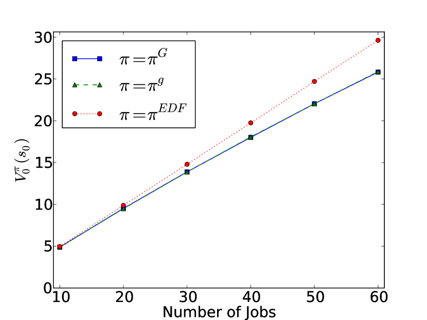
(a) Step-wise decay, Geometric PMFs

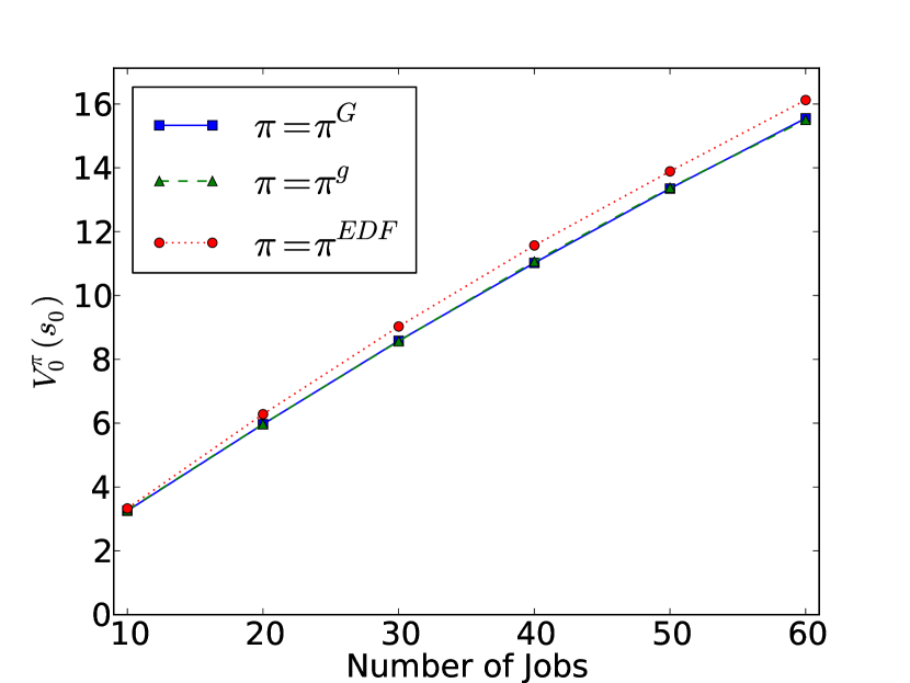
(b) Heterogeneous decay, Geometric PMFs

(c) Step-wise decay, Heterogeneous PMFs

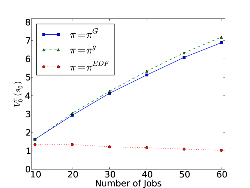
(d) Heterogeneous decay, Heterogeneous PMFs

Performance of $\pi^{G}$, $\pi^{g}$, and $\pi^{EDF}$ when $a=1$ and $(b,c)$ is random.We compare the performance of the heuristics when $N=5$ and $T=50$ while varying $J$.

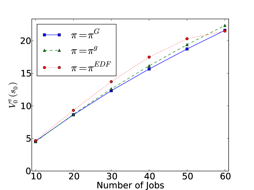
(a) Step-wise decay, Geometric PMFs

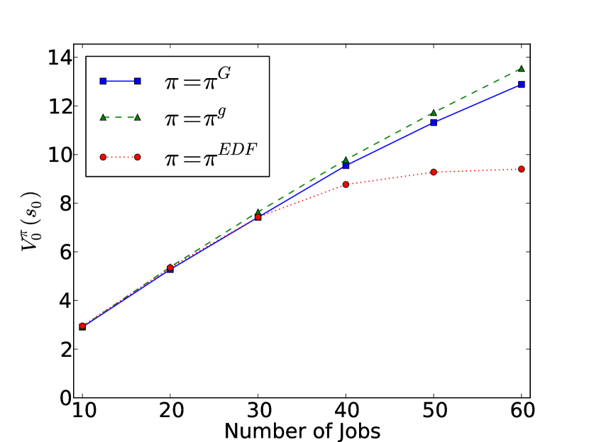
(b) Heterogeneous decay, Geometric PMFs

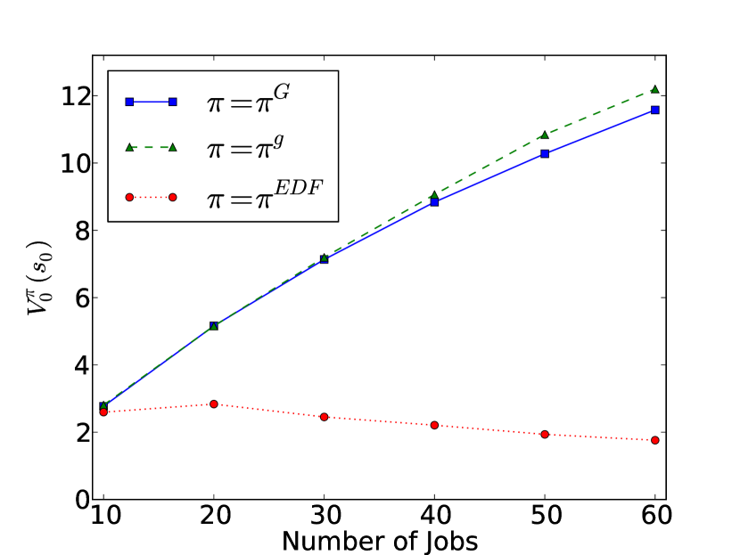
(c) Step-wise decay, Heterogeneous PMFs

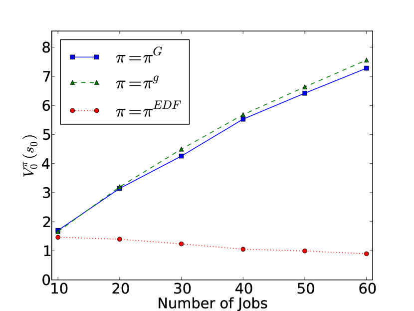
(d) Heterogeneous decay, Heterogeneous PMFs

Performance of $\pi^{G}$, $\pi^{g}$, and $\pi^{EDF}$ when $(a,b,c)$ is random.We compare the performance of the heuristics when $N=5$ and $T=50$ while varying $J$.

In Figure 1(a) we have geometric PMFs and step-wise value decay while in Figure 1(b) we have geometric PMFs and heterogeneous value decay. Note that in these cases, $\pi^{g}$ and $\pi^{G}$ are equivalent. In both plots we see that the value associated with each of the three heuristic policies increases as the number of jobs increases. This shows that when the service times are geometric, all three heuristics can manage increasing congestion reasonably well. An interesting feature of these plots is that $\pi^{EDF}$ outperforms $\pi^{g}$ and $\pi^{G}$. This matches our intuition from Example 3.3 and the small-scale simulation from the previous section. In the previous section, we saw that $\pi^{EDF}$ performed best when the PMFs were (truncated) geometrics. Recall that in Example 3.3, when $\mathbb{P}(\sigma=1)$ is close to 1, $\pi^{EDF}$ outperforms $\pi^{g}$ and $\pi^{G}$. Because $(1-1/e)\approx 0.63$, the probability of a job completing in one time slot is indeed qualitatively close to 1. In these examples, all of the jobs are very likely to finish in a short amount of time and since $\pi^{EDF}$ prioritizes time-critical jobs, $\pi^{EDF}$ does very well. Note that $\pi^{g}$ and $\pi^{G}$ also perform well. Furthermore, when the value decay functions are heterogeneous, the performance gap between $\pi^{g}/\pi^{G}$ and $\pi^{EDF}$ is quite small. These plots show that while it may be slightly better to use $\pi^{EDF}$ when the service times are short (with high probability), $\pi^{g}$ and $\pi^{G}$ are both good options as well.

In Figure 1(c) we have heterogeneous PMFs and step-wise value decay while in Figure 1(d) we have heterogeneous PMFs and heterogeneous value decay. Note that in these cases, the performance guarantee for $\pi^{EDF}$ does not apply because the service times are not identically distributed. We see that $\pi^{EDF}$ performs quite poorly and the value associated with $\pi^{EDF}$ does not increase as $J$ is increased. This demonstrates that with heterogeneous PMFs, $\pi^{EDF}$ does not handle congestion well. With heterogeneous PMFs, there are some jobs which will complete quickly, but many of the jobs will not. The results in Figure 4.1.2 demonstrate that the EDF policy is sensitive to the underlying service time distributions: $\pi^{EDF}$ will perform well when there is a high probability that the jobs will each complete in a single time slot, but otherwise $\pi^{EDF}$ will perform quite poorly. In contrast, both $\pi^{g}$ and $\pi^{G}$ perform well in the heterogeneous environments and are able to gain a greater reward as $J$ increases. In Figure 1(c), we see that $\pi^{g}$ and $\pi^{G}$ perform nearly identically until $J>30$. For $J>30$, $\pi^{g}$ performs slightly better than $\pi^{G}$. In Figure 1(d), this dichotomy becomes evident when $J>10$. This suggests that though $\pi^{g}$ and $\pi^{G}$ perform similarly for small problems, $\pi^{g}$ will be better when the system is more congested. Furthermore, the benefit of $\pi^{g}$ over $\pi^{G}$ is more evident when there is greater heterogeneity amongst the jobs.

Figure 4.1.2 (the case in which the parameter $a$ is randomly chosen for each job rather than being fixed), shows many of the same trends as Figure 4.1.2 but gives us additional insights into how heterogeneity in service times affects each heuristic policy. First note that each subfigure in Figure 4.1.2 shows that $\pi^{g}$ outperforms $\pi^{G}$ and that the difference in performance increases as $J$ increases. This demonstrates that for large numbers of jobs $\pi^{g}$ is superior to $\pi^{G}$. In Figure 1(a) and Figure 1(b), we saw that $\pi^{EDF}$ gained more rewards as $J$ increased. However, in Figure 2(a) and Figure 2(b) we see that the value associated with $\pi^{EDF}$ saturates as $J$ increases while the values associated with $\pi^{G}$ and $\pi^{g}$ do not. This supports the idea that $\pi^{EDF}$ is not nearly as robust as $\pi^{g}$ and $\pi^{G}$. Although $\pi^{EDF}$ can perform well, it may be more prudent to apply $\pi^{g}$ or $\pi^{G}$. Futhermore, for larger problems it may be best to use $\pi^{g}$ rather than $\pi^{G}$.

4.1.3 Rules-of-Thumb

Our numerical experiments and theoretical results have revealed several insights into the general problem of non-preemptive scheduling of jobs with decaying value. We summarize these insights with the following rules-of-thumb:

• The rate greedy policy has the best performance guarantee. The greedy policy has a better performance guarantee than EDF. In this sense, rate greedy policy is the most robust to changes in the underlying system parameters.

• For problems with relatively short time horizons, the greedy policy performs best.

• Despite the seemingly weak performance guarantee, EDF performs well under long time horizons when there is a high probability that the service times are short. In these situations, the rate greedy and greedy policies also perform very well, but EDF can perform even better.

• When the service times are large with high probability and/or if the reward decay function cannot be characterized by deadlines, EDF performs poorly. In these cases, it is better to use one of the greedy policies.

• For problems with long time horizons and heterogenous service time distributions , the rate greedy policy performs slightly better than the greedy policy. This difference is more pronounced when the reward decay functions are also heterogeneous.

4.2 Patient Scheduling in a Disaster Scenario

We now consider a patient scheduling problem where patients are “jobs” and operating rooms in a surgical center are “servers”. We are concerned with the 24 hour period immediately after a mass casualty incident as studies have shown that this is a critical period for hospitals responding to mass casualty incidents (e.g. Aylwin et al. (2007), Turégano-Fuentes et al. (2008a, b)). The random service times correspond to uncertainty in procedure durations and the internal value decay corresponds to the deterioration of patient health due to scheduling delays. For example, recall the “health score” used by Sacco et al. (2005) to model the decline in patient health as procedures are delayed. We consider a clearing system which is often used to model mass casualty incidents (e.g. Argon et al. (2011) and Chan et al. (2013)). Our model does not explicitly consider the details of a surgical operation (e.g. the pre-operative and post-operative phases), but does address the key dilemma of scheduling and prioritizing patients when there is a scarcity of operating rooms. Sub-optimal operating room schedules can lead to delays even in typical circumstances (Wachtel and Dexter 2009) and a spike in demand due to a disaster will only exacerbate this issue, so our model is able to capture a primary operational concern.

For the service time distributions, we use lognormal distributions. Strum et al. (2000) showed that lognormal distributions model surgical procedure times better than normal distributions. Furthermore, Spangler et al. (2004) demonstrated how to fit the parameters of a lognormal distribution to surgical data from hospitals. The use of lognormal distribution in modeling surgical procedure times is now quite common (e.g. Mihaylova et al. (2011)). We have elected to calibrate our simulation according to surgical procedures because these types of procedures are common when managing mass casualty incidents, e.g. during civilian terrorist attacks (Frykberg 2004) and in the aftermath of military combat (King and Jatoi 2005).

Because we have a discrete-time model, we need to discretize the lognormal density. Given parameters $\ell$, $m$, $s$, and a standard normal random variable $Z$, $\sigma$ is lognormal if

$$\sigma=\ell+e^{m+sZ}.$$ (9)

We will assume that $\sigma$ is measured in minutes. Given a time discretization $\delta$ and a number of time slots $T$, we can compute a PMF $p_{ln}(\cdot)$ which approximates the density of $\sigma$. See the appendix for details.

For each patient, we fix $\ell=60$, randomly select $m$ from a uniform distribution on $[1.0,4.0]$, and randomly select $s$ from a uniform distribution on $[1.0,1.25]$. With these parameters, expected procedure times are on the order of two to three hours, and the coefficient of variation for each procedure is between 0.1 and 1.5. This range for the coefficients of variation is motivated by Spangler et al. (2004) who showed that when fitting lognormal random variables to surgical procedure times, nearly procedures studied had coefficients of variation less than 1.5. While the study by Spangler et al. (2004) was not motivated by disaster scenarios, we note that there is an inherent difficulty in fitting statistical models to the types of procedures which arise during mass casualty incidents. Frykberg (2004) points out that the procedures required during mass casualty incidents are characterized by “complex and difficult wounding patterns that are not typically seen in routine practice” and that the rare nature of these procedures makes controlled statistical analysis difficult to perform. Consequently, while the selected parameter ranges are reasonable and somewhat plausible, one would need to make more judicious parameter choices in order to model specific scenarios. Incorporating expert knowledge can be useful when a data driven approach is not feasible and as mentioned before, one could apply the Delphi method (Linstone et al. 1975) to build models for specific disasters and injury types.

We consider a 24 hour period discretized into 10 minute time slots so that $\delta=10$ and $T=144$. We assume there are 6 operating rooms (the average number of operating rooms in a hospital in the United States according to Gallup (2001)) and that the medical resources are sufficient to complete operations at a constant rate. We assume that the time between procedures is negligible. If we assume that preparations such as the application of anesthesia are included in the service time distribution (as is done in Spangler et al. (2004)), then this is a fairly benign assumption.

Motivated by Sacco et al. (2005), we consider continuous piecewise linear value decay. Recall that in Sacco et al. (2005), a panel of expert physicians developed a deterministic mechanism for scoring how patients’ health decays over time. As shown earlier in Figure 1, the health scores decay continuously and in a piecewise linear fashion. Maximizing patient health is one way of optimizing quality of care, so our notion of value is analogous to the health score from Sacco et al. (2005). Mathematically, we can write such a value decay function as follows. The interval $[0,T]$ is divided into $I$ disjoint intervals such that

$$v_{pl}(t)=\sum_{i=0}^{I-1}(a_{i}t+b_{i})\mathbf{1}_{\left\{t_{i}\leq t\leq t_{i+1}\right\}}$$

where $\left\{a_{i}\right\}_{i=0}^{I-1}$ are non-positive constants and $\left\{b_{i}\right\}_{i=0}^{I-1}$ are non-negative constants. We additionally require

$$a_{i}t_{i+1}+b_{i}=a_{i+1}t_{i+1}+b_{i+t}$$

so that $v_{pl}(\cdot)$ is continuous. For each patient, we randomly select $\left\{a_{i}\right\}_{i=0}^{I-1}$ and $\left\{b_{i}\right\}_{i=0}^{I-1}$ with an algorithm detailed in the appendix. An example of a continuous piecewise linear value decay function is shown in Figure 4.2.

A plot of a piecewise linear value decay function. The patient has a health score (i.e. internal value) that is initially positive and less than 1. As the patient awaits treatment, this health score decreases in a continuous piecewise linear fashion. This kind of health decay model hsa been used in the medical literature, for example in Sacco et al. (2005).

We vary the number of patients $J\in\left\{50,75,100,\ldots,200\right\}$ and compare the performance of $\pi^{G}$, $\pi^{g}$, and $\pi^{EDF}$. Depending on the type of incident, the number of patients could range from tens (e.g. Aylwin et al. (2007), Turégano-Fuentes et al. (2008a, b)) to hundreds (e.g. Cushman et al. (2003)), so this is a reasonable range for $J$. For each $J$, we repeat the simulation $1000$ times and report the average. In addition to reporting $V^{\pi}_{0}(s_{0})$, we also report the fraction of patients who are served by their final deadline. The results are shown in Figure 4.2.

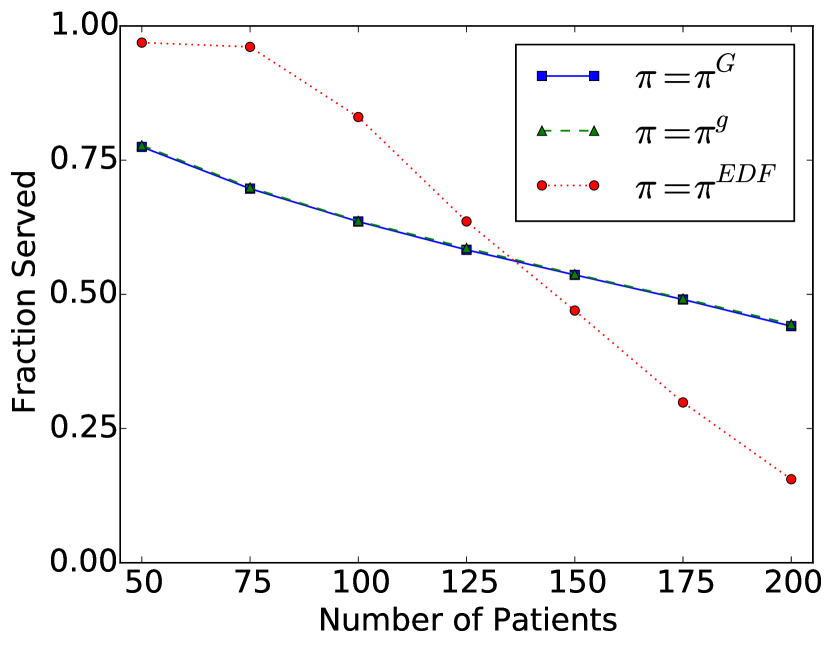
(a)

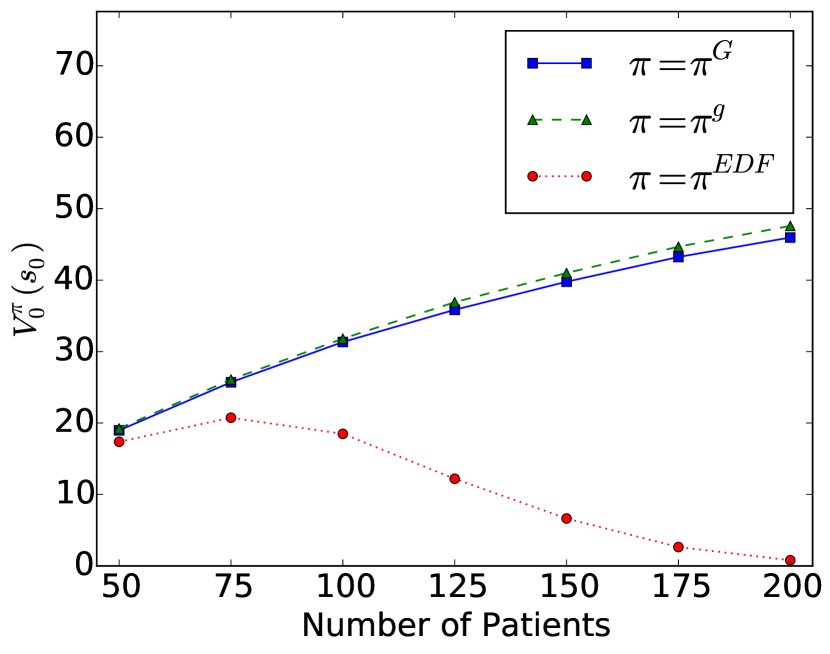
(b)

Performance of $\pi^{G}$, $\pi^{g}$, and $\pi^{EDF}$ in a patient scheduling scenario. We compare the performance of the heuristics when there are $N=6$ operating rooms and $T=144$ time slots of $\delta=10$ minute duration (i.e. 24 hours divided into 10 minute time slots). The patients have piecewise linear value decay and discretized lognormal service times. The parameters which characterize each patient are chosen randomly. We increase the number of patients $J\in\left\{50,75,100,\ldots,200\right\}$ and for each $J$ we report the average of $1000$ simulations. In addition to reporting $V_{0}^{\pi}(s_{0})$, we also report the fraction of patients who are served by their final deadline.

For $\pi^{G}$ and $\pi^{g}$, we see some expected trends: as $J$ increases, both policies increase in value while the fraction of patients served gradually decreases. As with our other “large-scale” numerical experiments, $\pi^{g}$ performs slightly better than $\pi^{G}$. The results for $\pi^{EDF}$ are more nuanced. For $J\leq 75$, the value associated with $\pi^{EDF}$ is less than that of $\pi^{G}$ and $\pi^{g}$, but only slightly. However, for $J\leq 75$, $\pi^{EDF}$ serves more than $95\%$ all patients. As a result, for $J\leq 75$, $\pi^{EDF}$ is better at preventing mortality than $\pi^{G}$ or $\pi^{g}$ though potentially at the cost of lower quality of care. While this is a positive result, we see a decrease in performance when $J$ increases beyond $100$. For $J\geq 100$, the value of $\pi^{EDF}$ and the fraction of patients served decreases substantially. While $\pi^{G}$ and $\pi^{g}$ decay in performance gradually as $J$ increases, $\pi^{EDF}$ exhibits a phase transition from “good” performance to “poor” performance. Although the “critical point” of this phase transition is difficult to know a priori, this behavior can qualitatively be explained by the combination of piecewise linear value decay and lognormal service distributions. Because the patient characteristics are randomly generated, as $J$ increases, it becomes more likely that patients with early deadlines have long service times and low health values. This is due to the fact that the randomly generated piecewise linear value functions can decay quickly coupled with the fact that lognormal distributions are heavy-tailed. These patients occupy the operating rooms and block other patients from being scheduled. This causes many patients to not be served and for an overall low total value.

These results echo the results that we saw in our previous numerical experiments. Both $\pi^{G}$ and $\pi^{g}$ perform well and are reasonably robust. In contrast, $\pi^{EDF}$ can perform well sometimes but is not robust. In general, one will not know a priori where $\pi^{EDF}$ will experience its phase transition from good to bad performance. Because of this unpredictable behavior, for critical applications like patient scheduling it is probably best to avoid $\pi^{EDF}$. On the other hand, $\pi^{G}$ and $\pi^{g}$ are both good choices with $\pi^{g}$ being slightly better in large-scale scenarios.

5 Conclusion

We have presented a novel discrete-time model for non-preemptive scheduling. In this model, jobs have random service times and the value of each job decays deterministically. The jobs are dynamically scheduled on identical servers which each have unit service rate. We formulated the problem in a dynamic programming framework and showed that while an optimal scheduling policy exists, finding it is computationally intractable. This leads us to consider three low-complexity heuristics: a greedy policy, a rate greedy policy and an earliest-deadline-first (EDF) policy. In addition to providing performance guarantees (some of which are sharp), we have conducted extensive numerical experiments to compare the policies.

We have demonstrated that, in general, it is best to use the rate greedy policy; the greedy policy performs nearly as well as the rate greedy policy; and, EDF typically does not perform well at all. However, there are some scenarios in which EDF performs better than either greedy policy. Specifically, EDF performs better when the time horizon is long and all of the jobs have a high probability of completing service in a short amount of time. In all other situations which we considered, EDF performs poorly. In particular, our simulations suggest that in patient scheduling scenarios, it is best to use the rate greedy policy. We find that it would be reasonable to use the greedy policy, but EDF likely should be avoided.

Our insights also point us to other research topics of potential interest. For example, although the heuristics considered in this work can be applied even when there are job arrivals, our performance guarantees would no longer be valid. Incorporating job arrivals would be a slight modeling extension but it would drastically change our analysis. In particular, our proofs apply backwards induction to the number of jobs in the system. This requires that the number of jobs in the system is non-increasing which would clearly be violated if there were arrivals. We could also consider a model in which job value decays stochastically. This would be useful for situations in which our understanding of the internal job dynamics is imperfect so we only have a distribution on the value dynamics. In addition to considering modeling extensions, within this same model we could consider many other myopic heuristics which could be relevant to other applications. As noted above, the proofs can easily be adapted and extended to other myopic scheduling policies which may be useful for other applications.

Neal Master is funded by Stanford University through a Stanford Graduate Fellowship (SGF) in Science & Engineering.

6 Preliminary Mathematical Definitions and Results

6.1 Definitions

In addition to the notation in Section 2.1, we introduce the following notation.

Given a random variable $X$ the conditional value function for a policy $\pi$ is

$$V_{t}^{\pi}(s|X)=\mathbb{E}\left[\left.\sum_{\tau=t}^{\infty}R_{\tau}(s_{\tau},\pi_{\tau}(s_{\tau}))\right|X\right].$$

If we want to condition on an event $E$, take $X=\mathbf{1}_{\left\{E\right\}}$ and let $V_{t}^{\pi}(s|E)=V_{t}^{\pi}(s|X)\mathbf{1}_{\left\{X=1\right\}}$.

If $s=(b(t),p(t))$ then we let $\mathbf{b}(s)=b(t)$ and $\mathbf{p}(s)=p(t)$.

6.2 Proof of Theorem 2.1

If for some finite $T$ we have $b(T)=(\top,\top,\ldots,\top)$, then $p(T)=(0,0,\ldots,0)$ and $s_{T}=(b(T),p(T))$ is a no cost/reward trapping state. If we fix any non-idling policy, because $\mathbb{E}[\sigma_{j}]<\infty$ for all $j\in\mathcal{J}$, there is an associated finite stopping time $T$ at which $b(T)=(\top,\top,\ldots\top)$. Therefore, we have a stochastic shortest path problem with destination state $s_{T}$. The system will reach $s_{T}$ in a finite amount of time and so the given policy is proper. This guarantees the existence of an optimal policy which is obtainable via policy iteration (Bertsekas 2012, Proposition 3.2.2).   $\Halmos$

6.3 Proof of Theorem 2.2

Consider a particular instance of the problem in which $\sigma_{j}$ is known with probability 1 and $v_{j}(t)=c_{j}\mathbf{1}_{\left\{t\leq K\right\}}$ for some fixed constants $\left\{c_{j}\right\}$ and $K$. In this case, the job service times are essentially deterministic and the jobs have a shared deadline. This is a 0/1 Multiple Knapsack Problem in which there are $J$ objects with sizes $\left\{\sigma_{j}\right\}$ and values $\left\{c_{j}\right\}$ which need to be placed in $N$ knapsacks each with capacity $K$. This particular instance of the problem is NP-hard (see Martello and Toth (1990) and the references therein) so the problem of computing an optimal policy is NP-hard.   $\Halmos$

7 Some Useful Lemmas

We will now prove a few lemmas which will be useful when proving the main results of the papers.

Intuitively, if there are more jobs in the system, then there are more scheduling choices available and an optimal policy will be able to accrue a greater reward. This intuition is formalized in the following lemma.

Lemma 7.1 (Monotonicity in Jobs)

Consider states $s$ and $s^{\prime}$ which are related by the three following conditions:

$$\mathbf{b}(s^{\prime})_{j}\not\in\left\{\bot,\top\right\}\implies\mathbf{b}(s^{\prime})_{j}=\mathbf{b}(s)_{j};\quad\mathbf{b}(s^{\prime})_{j}=\bot\implies\mathbf{b}(s)_{j}=\bot;\quad\mathbf{p}(s^{\prime})=\mathbf{p}(s)$$

Then $V_{t}^{*}(s)\geq V_{t}^{*}(s^{\prime})$.

Proof 7.2

Proof. Consider a coupling of two systems each starting at $s$ and $s^{\prime}$ such that they see the same realizations of service times $\left\{\sigma_{j}\right\}_{j\in\mathcal{J}}$. Let $\mathcal{J}_{s^{\prime}}=\left\{j\in\mathcal{J}:\mathbf{b}(s^{\prime})_{j}\neq\top\right\}$ and $\mathcal{J}_{s}=\left\{j\in\mathcal{J}:\mathbf{b}(s)_{j}\neq\top\right\}$. Note that $\mathcal{J}_{s^{\prime}}\subseteq\mathcal{J}_{s}$.

Let $\pi^{*}$ be an optimal policy. We assume that $\pi^{*}$ is applied to the $s^{\prime}$-system. Consider the following suboptimal policy $\tilde{\pi}$ which is used for the $s$-system: $\tilde{\pi}$ takes the same actions as $\pi^{*}$ until all the jobs $j\in\mathcal{J}_{s^{\prime}}$ are completed and then completes jobs $j\in\mathcal{J}_{s}\setminus\mathcal{J}_{s^{\prime}}$ in sequential order. Let $T_{j}$ be the completion time of job $j$ in the $s$-system when using policy $\tilde{\pi}$. Let $T_{j}^{*}$ be the completion time of job $j$ in the $s^{\prime}$-system using the policy $\pi^{*}$. The coupling ensures that $T_{j}=T_{j}^{*}$ for all $j\in\mathcal{J}_{s^{\prime}}$.

$$V_{t}^{\tilde{\pi}}(s|\sigma_{1},\ldots,\sigma_{J}) =\sum_{j\in\mathcal{J}_{s}}v_{j}(T_{j})=\sum_{j\in\mathcal{J}_{s^{\prime}}}v_{j}(T_{j})+\sum_{j\in\mathcal{J}_{s}\setminus\mathcal{J}_{s^{\prime}}}v_{j}(T_{j})=\sum_{j\in\mathcal{J}_{s^{\prime}}}v_{j}(T_{j}^{*})+\sum_{j\in\mathcal{J}_{s}\setminus\mathcal{J}_{s^{\prime}}}v_{j}(T_{j})$$

$$\geq\sum_{j\in\mathcal{J}_{s^{\prime}}}v_{j}(T_{j}^{*})=V_{t}^{*}(s^{\prime}|\sigma_{1},\ldots,\sigma_{J})$$

Taking the expectation gives us that $V_{t}^{\tilde{\pi}}(s)\geq V_{t}^{*}(s^{\prime})$. The optimality of $V^{*}$ tells us that $V_{t}^{*}(s)\geq V_{t}^{\tilde{\pi}}(s)$ so we can conclude that $V_{t}^{*}(s)\geq V_{t}^{*}(s^{\prime})$.   $\Halmos$

Because the internal value of the jobs decays over time, one would expect an optimal policy to be non-idling. Our next lemma shows that it is sufficient to focus our attention on non-idling policies. Note that because of Lemma 7.3, we will assume throughout that any optimal policy is non-idling.

Lemma 7.3 (Non-idling)

Suppose that in state $s_{t}$, there are $M=\left|\left\{n\in\mathcal{N}:\mathbf{p}(s)_{n}=0\right\}\right|$ free machines and that the number of jobs remaining to be processed is $K=\left|\left\{j\in\mathcal{J}:\mathbf{b}(s)_{j}=\bot\right\}\right|$. Then there exists an optimal policy $\pi^{*}$ such that $\pi^{*}_{t}(s)$ schedules $\min\left\{K,M\right\}$ jobs.

Proof 7.4

Proof. Let $A=\pi^{*}_{t}(s_{t})$. We show that nothing can be gained by having $\left|A\right|<\min\left\{K,M\right\}$. Suppose under $\pi^{*}$ that a processor remains idle even though there is an available job. Consider another policy $\pi^{\prime}$ which schedules identically to $\pi^{*}$ except it begins processing all jobs on the idling machine one time slot earlier. Since $v_{j}(\cdot)$ is non-increasing, $V_{t}^{\pi^{\prime}}(s)\geq V_{t}^{*}(s)$. Therefore, $\pi^{\prime}$ is also optimal and does not idle.   $\Halmos$

Consider a “virtual machine” which is able to complete jobs instantaneously. Intuitively, such a virtual machine would allow for a greater total expected reward. Our next lemma justifies this intuition.

Lemma 7.5 (Virtual Machine Rewards)

Fix a state $s$ and a job $i$ such that $\mathbf{b}(s)_{i}=\bot$. Let $s^{\prime}_{i}=S^{\prime}(s,i)$ denote the resulting state if job $i$ were processed without occupying a processor. In notation,

$$\mathbf{b}(s)_{i}=\bot,\quad\mathbf{b}(s^{\prime}_{i})_{i}=\top,\quad\mathbf{p}(s)=\mathbf{p}(s^{\prime}_{i}),\quad\mathbf{b}(s^{\prime}_{i})_{j}=\mathbf{b}(s)_{j}\,\forall\,j\in\mathcal{J}\setminus\left\{i\right\}.$$

Then $V_{t}^{*}(s)\leq\mathbb{E}[v_{j}(t+\sigma_{j})]+V_{t}^{*}(S^{\prime}(s,j))$.

Proof 7.6

Proof. Consider two systems starting in states $s$ and $S^{\prime}(s,j)$ respectively. We couple the systems so that they see the same realizations of the services times. We assume that the $s$-system evolves under an optimal policy $\pi^{*}$. Let $\left\{t_{j}^{*}\right\}$ be the random times are which jobs $j\in\mathcal{J}_{s}=\left\{j\in\mathcal{J}:\mathbf{b}(s)_{j}=\bot\right\}$ begin processing. Let $\pi^{\prime}$ be the policy for the $s_{i}^{\prime}$-system. Let $\left\{t_{j}^{\prime}\right\}$ be the random times at which job $j\in\mathcal{J}^{\prime}=\left\{j\in\mathcal{J}:\mathbf{b}(s_{i}^{\prime})_{j}=\bot\right\}$. We assume that $\pi^{\prime}$ mimics $\pi^{*}$ as follows. Policy $\pi^{\prime}$ takes the same actions as $\pi^{*}$ for all jobs $j\in\mathcal{J}^{\prime}$ and when $\pi^{*}$ would be processing job $i$, $\pi^{\prime}$ idles. Therefore, $t_{j}^{\prime}=t_{j}^{*}$ for all $j\in\mathcal{J}^{\prime}$:

$$V_{t}^{*}(s) =\mathbb{E}\left[\sum_{j\in\mathcal{J}_{s}}v_{j}(t_{j}^{*}+\sigma_{j})\right]=\mathbb{E}\left[\sum_{j\in\mathcal{J}_{s}\setminus\left\{i\right\}}v_{j}(t_{j}^{*}+\sigma_{j})\right]+\mathbb{E}[v_{i}(t_{i}^{*}+\sigma_{i})]$$

$$=\mathbb{E}\left[\sum_{j\in\mathcal{J}^{\prime}}v_{j}(t_{j}^{\prime}+\sigma_{j})\right]+\mathbb{E}[v_{i}(t_{i}^{*}+\sigma_{i})]=V_{t}^{\pi^{\prime}}(s_{i}^{\prime})+\mathbb{E}[v_{i}(t_{i}^{*}+\sigma_{i})]\leq V_{t}^{*}(s_{i}^{\prime})+\mathbb{E}[v_{i}(t+\sigma_{i})]$$

The final inequality follows from the optimality of $V_{t}^{*}(s_{i}^{\prime})$ and the non-decreasing nature of $v_{i}(\cdot)$.   $\Halmos$

8 Proof of Theorem 3.7

The proof of the performance bound for $\pi^{g}$ is slightly more complicated than the proofs required for $\pi^{G}$ and $\pi^{EDF}$. However, the proofs are structurally similar and so the later appendices will modify the proof presented here. We first need to prove the following lemma which shows how sub-optimal scheduling of “replica” jobs can affect the performance of the system.

Lemma 8.1

Consider an augmented set of jobs $\tilde{\mathcal{J}}=\mathcal{J}\cup\left\{\tilde{g},\tilde{i}\right\}$ where $\tilde{g}$ is a replica of some job $g$ and $\tilde{i}$ is a replica of some job $i$. By replica, we mean that $\sigma_{\tilde{g}}\overset{d}{=}\sigma_{g}$ and $\sigma_{\tilde{i}}\overset{d}{=}\sigma_{i}$ but that $v_{\tilde{g}}(t)=v_{\tilde{i}}(t)=0$.

Consider a state $s_{t}=s$ at time $t$. Let $\mathcal{J}_{s}=\left\{j\in\mathcal{J}:\mathbf{b}(s)_{j}\neq\top\right\}$ and fix $g\in\argmax_{j\in\mathcal{J}_{s}}\frac{\mathbb{E}[v_{j}(t+\sigma_{j})]}{\mathbb{E}[\sigma_{j}]}$. Assume that for some $f\in\mathcal{N}$, $\mathbf{p}(s)_{f}=0$ (i.e. processor $f$ is free).

Denote by $s_{g}$ and $s_{i}$ two states which are related to state $s$ in the following manner. The two states are identical to state $s$ except on machine $f$. In state $s_{g}$, machine $f$ is occupied by the replica $\tilde{g}$ so that $\mathbf{p}(s_{g})_{f}=\tilde{g}$. Similarly for state $s_{i}$, $\mathbf{p}(s_{i})_{f}=\tilde{i}$. Then

$$V_{t}^{*}(s_{i})\leq\left(1+\frac{\mathbb{E}[\max_{j\in\mathcal{J}_{s}}\sigma_{j}]}{\mathbb{E}[\sigma_{g}]}-\frac{\mathbb{E}[\sigma_{i}]}{\mathbb{E}[\sigma_{g}]}\right)\mathbb{E}[v_{g}(t+\sigma_{g})]+V_{t}^{*}(s_{g}).$$

Note that because the replica jobs do not generate any rewards, the augmented system can be optimally controlled by a policy that is essentially the same as an optimal policy for the original system. If we take any optimal policy for the original system, we can create an optimal policy for the augmented system as follows: take the same actions as the given optimal policy until all jobs in $\mathcal{J}$ have completed; then complete the replica jobs. Since the replica jobs have no reward, the optimal value is the same in both systems. As a result we will abuse notation and use $V_{t}^{*}(\cdot)$ as the optimal value function for all systems in Lemma 8.1.

Proof 8.2

Proof of Lemma 8.1. We begin by coupling the systems such that they see the same realizations for service times. Consider a policy $\pi_{g}^{\prime}$ for the $s_{g}$-system which attempts to mimic the actions taken by an optimal policy $\pi_{i}^{*}$ on the $s_{i}$-system. There are two possible cases, $\sigma_{\tilde{i}}\geq\sigma_{\tilde{g}}$ and $\sigma_{\tilde{i}}<\sigma_{\tilde{g}}$.

• Case 1, $\sigma_{\tilde{i}}\geq\sigma_{\tilde{g}}$: After job $\tilde{g}$ has completed, the $\pi_{g}^{\prime}$ policy idles on machine $f$ until $t+\sigma_{\tilde{i}}$ (time which machine $f$ is free in the $s_{i}$-system). At this point, the $s_{g}$-system is “synced” with the $s_{i}$-system and it proceeds with executing the optimal policy for the $s_{i}$ system, $\pi_{i}^{*}$.

  If $T_{j}^{*}(s_{i})$ is the completion time of job $j$ in the $s_{i}$-system under optimal policy $\pi_{i}^{*}$, and $T_{j}$ is the completion time of job $j$ in the $s_{g}$-system under the $\pi_{g}^{\prime}$, then $T_{j}=T_{j}^{*}(s_{i})$ for all $j\in\mathcal{J}_{s}$.

  $$\begin{split}V_{t}^{*}(s_{i}|\sigma_{\tilde{i}}\geq\sigma_{\tilde{g}})&=\mathbb{E}\left[\left.\sum_{j\in\mathcal{J}_{s}}v_{j}(T_{j}^{*}(s_{i}))\right|\sigma_{\tilde{i}}\geq\sigma_{\tilde{g}}\right]=\mathbb{E}\left[\left.\sum_{j\in\mathcal{J}_{s}}v_{j}(T_{j})\right|\sigma_{\tilde{i}}\geq\sigma_{\tilde{g}}\right]=V_{t}^{\pi_{g}^{\prime}}(s_{g}|\sigma_{\tilde{i}}\geq\sigma_{\tilde{g}})\\ &\leq V_{t}^{*}(s_{g}|\sigma_{\tilde{i}}\geq\sigma_{\tilde{g}})\\ &\leq V_{t}^{*}(s_{g}|\sigma_{\tilde{i}}\geq\sigma_{\tilde{g}})+\left(1+\frac{\mathbb{E}[\max_{j\in\mathcal{J}_{s}}\sigma_{j}]}{\mathbb{E}[\sigma_{g}]}-\frac{\mathbb{E}[\sigma_{i}]}{\mathbb{E}[\sigma_{g}]}\right)\mathbb{E}[v_{g}(t+\sigma_{g})]\end{split}$$ (10)

  The inequalities come from the construction of $\pi_{g}^{\prime}$ and the fact that the added term is non-negative.

• Case 2, $\sigma_{\tilde{i}}<\sigma_{\tilde{g}}$: In this case, $\pi_{g}^{\prime}$ cannot exactly mimic $\pi_{i}^{*}$ policy because machine $f$ will continue to be busy after $\tilde{i}$ completes in the $s_{i}$-system. While machine $f$ is processing $\tilde{g}$ in the $s_{g}$-system, machine $f$ will process jobs $\mathcal{J}_{sim}$ in the $s_{i}$-system. The $\pi_{g}^{\prime}$ policy will “simulate” the processing of the jobs in $\mathcal{J}_{sim}$ while they are actually being processed in the $s_{i}$-system. After job $\tilde{g}$ is completed in the $s_{g}$-system, $\pi_{g}^{\prime}$ will continue to mimic $\pi_{i}^{*}$ as if the simulated jobs were actually completed. When $\pi_{i}^{*}$ has completed all jobs in the $s_{i}$-system, $\pi_{g}^{\prime}$ will then complete jobs in $\mathcal{J}_{sim}$ in the $s_{g}$-system in some arbitrary order.

  If $T_{j}^{*}(s_{i})$ is the completion time of job $j$ in the $s_{i}$-system under optimal policy, $\pi_{i}^{*}$ and $T_{j}$ is the completion time of job $j$ in the $s_{g}$-system under the $\pi_{g}^{\prime}$ policy, then $T_{j}=T_{j}^{*}(s_{i})$ for all $j\in\mathcal{J}\setminus\mathcal{J}_{sim}$.

  $$\begin{split}V_{t}^{*}(s_{i}|\sigma_{\tilde{i}}<\sigma_{\tilde{g}})&=\mathbb{E}\left[\left.\sum_{j\in\mathcal{J}_{s}}v_{j}(T_{j}^{*}(s_{i}))\right|\sigma_{\tilde{i}}<\sigma_{\tilde{g}}\right]\\ &=\mathbb{E}\left[\left.\sum_{j\in\mathcal{J}_{sim}}v_{j}(T_{j}^{*}(s_{i}))+\sum_{j\not\in\mathcal{J}_{sim}}v_{j}(T_{j}^{*}(s_{i}))\right|\sigma_{\tilde{i}}<\sigma_{\tilde{g}}\right]\\ &\leq\mathbb{E}\left[\left.\sum_{j\in\mathcal{J}_{sim}}v_{j}(T_{j}^{*}(s_{i}))+\sum_{j\not\in\mathcal{J}_{sim}}v_{j}(T_{j}^{*}(s_{i}))+\sum_{j\in\mathcal{J}_{sim}}v_{j}(T_{j})\right|\sigma_{\tilde{i}}<\sigma_{\tilde{g}}\right]\\ &=\mathbb{E}\left[\left.\sum_{j\in\mathcal{J}_{sim}}v_{j}(T_{j}^{*}(s_{i}))\right|\sigma_{\tilde{i}}<\sigma_{\tilde{g}}\right]+V_{t}^{\pi_{g}^{\prime}}(s_{g}|\sigma_{\tilde{i}}<\sigma_{\tilde{g}})\\ &\leq\mathbb{E}\left[\left.\sum_{j\in\mathcal{J}_{sim}}v_{j}(T_{j}^{*}(s_{i}))\right|\sigma_{\tilde{i}}<\sigma_{\tilde{g}}\right]+V_{t}^{*}(s_{g}|\sigma_{\tilde{i}}<\sigma_{\tilde{g}})\end{split}$$ (11)

  The first equality follows by definition. The second equality follows because $\mathcal{J}_{s}=\mathcal{J}_{sim}\cup\mathcal{J}_{sim}^{c}$. The inequality comes from the non-negativity of $v_{j}(\cdot)$. The final two equalities follow from the construction of $\pi_{g}^{\prime}$.

  Continuing, note that at the earliest, job $j$ can be completed at $t+\sigma_{j}$ so $T_{j}^{*}(s_{i})\geq t+\sigma_{j}$. Since $v_{j}(\cdot)$ is non-decreasing, we have the following:

  $$\begin{split}V_{t}^{*}(s_{i}|\sigma_{\tilde{i}}<\sigma_{\tilde{g}})&\leq\mathbb{E}\left[\left.\sum_{j\in\mathcal{J}_{sim}}v_{j}(T_{j}^{*}(s_{i}))\right|\sigma_{\tilde{i}}<\sigma_{\tilde{g}}\right]+V_{t}^{*}(s_{g}|\sigma_{\tilde{i}}<\sigma_{\tilde{g}})\\ &\leq\mathbb{E}\left[\left.\sum_{j\in\mathcal{J}_{sim}}v_{j}(t+\sigma_{j})\right|\sigma_{\tilde{i}}<\sigma_{\tilde{g}}\right]+V_{t}^{*}(s_{g}|\sigma_{\tilde{i}}<\sigma_{\tilde{g}})\end{split}$$ (12)

  Now focus on the first term. Since $\mathcal{J}_{sim}$ depends on the realizations of $\sigma_{\tilde{i}}$ and $\sigma_{\tilde{g}}$, it is a random set upon which we can condition.

  $$\mathbb{E}\left[\left.\sum_{j\in\mathcal{J}_{sim}}v_{j}(t+\sigma_{j})\right|\sigma_{\tilde{i}}<\sigma_{\tilde{g}},\mathcal{J}_{sim}\right] =\mathbb{E}\left[\left.\sum_{j\in\mathcal{J}_{sim}}\mathbb{E}[\sigma_{j}]\frac{v_{j}(t+\sigma_{j})}{\mathbb{E}[\sigma_{j}]}\right|\sigma_{\tilde{i}}<\sigma_{\tilde{g}},\mathcal{J}_{sim}\right]$$

  $$=\sum_{j\in\mathcal{J}_{sim}}\mathbb{E}[\sigma_{j}]\frac{\mathbb{E}[v_{j}(t+\sigma_{j})|\sigma_{\tilde{i}}<\sigma_{\tilde{g}},\mathcal{J}_{sim}]}{\mathbb{E}[\sigma_{j}]}$$

  $$\leq\sum_{j\in\mathcal{J}_{sim}}\mathbb{E}[\sigma_{j}]\frac{\mathbb{E}[v_{g}(t+\sigma_{g})]}{\mathbb{E}[\sigma_{g}]}=\frac{\mathbb{E}[v_{g}(t+\sigma_{g})]}{\mathbb{E}[\sigma_{g}]}\sum_{j\in\mathcal{J}_{sim}}\mathbb{E}[\sigma_{j}]$$

  The first equality is valid because $\sigma_{j}\geq 1$ and the second equality is an application of the linearity of conditional expectation. The final inequality is due to the fact that the index $g$ is chosen independently of $\sigma_{\tilde{i}}$, $\sigma_{\tilde{g}}$, and $\mathcal{J}_{sim}$.

  The maximum amount of time machine $f$ will idle in the $s_{g}$-system will be $\sigma_{\tilde{g}}-\sigma_{\tilde{i}}+\sigma_{max}$. Indeed, $\pi_{g}^{\prime}$ will need to simulate jobs for at least $\sigma_{\tilde{g}}-\sigma_{\tilde{i}}$ and one job may begin simulation just before $t+\sigma_{\tilde{g}}$. Applying this bound and taking the expectation of $\mathcal{J}_{sim}$ gives the following:

  $$\mathbb{E}\left[\left.\sum_{j\in\mathcal{J}_{sim}}v_{j}(t+\sigma_{j})\right|\sigma_{\tilde{i}}<\sigma_{\tilde{g}},\right] \leq\frac{\mathbb{E}[v_{g}(t+\sigma_{j})]}{\mathbb{E}[\sigma_{g}]}\mathbb{E}\left[\left.\sum_{j\in\mathcal{J}_{sim}}\mathbb{E}[\sigma_{j}]\right|\sigma_{\tilde{i}}<\sigma_{\tilde{g}}\right]$$

  $$\leq\frac{\mathbb{E}[v_{g}(t+\sigma_{j})]}{\mathbb{E}[\sigma_{g}]}\mathbb{E}[\sigma_{\tilde{g}}-\sigma_{\tilde{i}}+\sigma_{max}|\sigma_{\tilde{i}}<\sigma_{\tilde{g}}]$$

  So we have that

  $$V_{t}^{*}(s_{i}|\sigma_{\tilde{i}}<\sigma_{\tilde{g}})\leq\frac{\mathbb{E}[v_{g}(t+\sigma_{j})]}{\mathbb{E}[\sigma_{g}]}\mathbb{E}[\sigma_{\tilde{g}}-\sigma_{\tilde{i}}+\sigma_{max}|\sigma_{\tilde{i}}<\sigma_{\tilde{g}}]+V_{t}^{*}(s_{g}|\sigma_{\tilde{i}}<\sigma_{\tilde{g}}).$$ (13)

Now combine (10) and (13) and take the expectation over $\sigma_{\tilde{i}}\geq\sigma_{\tilde{g}}$ and $\sigma_{\tilde{i}}<\sigma_{\tilde{g}}$. Noting that $\sigma_{\tilde{i}}\overset{d}{=}\sigma_{i}$ and $\sigma_{\tilde{g}}\overset{d}{=}\sigma_{g}$ gives us the result:

$$V_{t}^{*}(s_{i})\leq\frac{\mathbb{E}[v_{g}(t+\sigma_{g})]}{\mathbb{E}[\sigma_{g}]}(\mathbb{E}[\sigma_{g}]-\mathbb{E}[\sigma_{i}]+\mathbb{E}[\sigma_{\max}])+V_{t}^{*}(s_{g})=\mathbb{E}[v_{g}(t+\sigma_{g})]\left(1+\frac{\mathbb{E}[\sigma_{max}]}{\mathbb{E}[\sigma_{g}]}-\frac{\mathbb{E}[\sigma_{i}]}{\mathbb{E}[\sigma_{g}]}\right)+V_{t}^{*}(s_{g})$$

$\Halmos$

Now we can prove the performance guarantee in Theorem 3.7. One of the key ideas of the proof is as follows: we will add replica jobs as in Lemma 8.1, apply the monotonicity result in Lemma 7.1, and make use of the virtual machines in Lemma 7.5 to complete the replicas. Because the replica jobs have no value, “adding and subtracting” these replicas does not impact the total value of system.

Proof 8.3

Proof of Theorem 3.7 The proof proceeds by induction on the number of jobs remaining to be processed, $\sum_{j\in\mathcal{J}}\mathbf{1}_{\{b_{j}(t)=\bot\}}$. The claim is trivially true if there is only one job remaining to be processed because $\pi^{g}$ and any (non-idling) $\pi^{*}$ will coincide. Now consider a state $s$ such that $\sum_{j}\mathbf{1}_{\{\mathbf{b}(s)_{j}=\bot\}}=K$, and assume that the claim is true for all states $s^{\prime}$ with $\sum_{j}\mathbf{1}_{\{\mathbf{b}(s^{\prime})_{j}=\bot\}}<K$.

Now if $\pi_{t}^{*}(s)=\pi_{t}^{g}(s)$ the then the next state encountered and rewards generated in both systems are identically distributed so that the induction hypothesis immediately yields the result for state $s$.

Consider the case where $\pi_{t}^{*}(s)\neq\pi_{t}^{g}(s)$. Let $A_{*}$ and $A_{g}$ denote the optimal and myopic scheduling policy, respectively, given state $s$ in time slot $t$. Denote by $\mathcal{J}_{*}$ and $\mathcal{J}_{g}$ the corresponding sets of jobs processed by the optimal and myopic policies in state $s$ at time $t$. We suppress the dependence on $s$ and $t$ for notational compactness. Recall that by Lemma 7.3, $|\mathcal{J}_{*}|=|\mathcal{J}_{g}|$. Furthermore, the free processors which are being assigned jobs define a bijection between $\mathcal{J}_{*}$ and $\mathcal{J}_{g}$. If we take $i\in\mathcal{J}_{*}$ then $g(i)\in\mathcal{J}_{g}$ is corresponding job. Similarly, if we take $g\in\mathcal{J}_{g}$ then $i(g)\in\mathcal{J}_{*}$ is the corresponding job. The myopic policy will select the $\left|\mathcal{J}_{g}\right|$ jobs with the largest reward rate. Since the processors are identical, we can therefore assume that jobs are matched to processors in a way so that $\frac{\mathbb{E}[v_{i}(t+\sigma_{i})]}{\mathbb{E}[\sigma_{i}]}\leq\frac{\mathbb{E}[v_{g(i)}(t+\sigma_{g(i)})]}{\mathbb{E}[\sigma_{g(i)}]}$.

Taking definitions from before, we define $\tilde{S}(s,A)$ as the random next state encountered given that we start in state $s$ and action $A$ is taken. Also, $S^{\prime}(s,i)$ is identical to state $s$ but with job $i$ is completed: $\mathbf{b}(S^{\prime}(s,i))_{i}=\top$.

Given a scheduling action $A$ and state $s$ at time $t$, we define the augmented state $\hat{s}=\hat{S}(s,A)$ as follows. Let $\mathcal{J}_{A}$ denote the jobs to be scheduled by $A$ and $\tilde{\mathcal{J}}_{A}$ to be replicas of these jobs. Recall that replica jobs have the same service requirements but no reward: if $j\in\mathcal{J}_{A}$ and $\tilde{j}\in\tilde{\mathcal{J}}_{A}$ is the replica, then $\sigma_{\tilde{j}}\overset{d}{=}\sigma_{j}$ and $v_{\tilde{j}}(\cdot)=0$. Then $\hat{s}$ is given by scheduling the replica jobs instead of the original jobs. In notation, $\mathbf{b}(\hat{s})_{j}=\mathbf{b}(s)_{j}$ for $j\in\mathcal{J}_{A}$, $\mathbf{b}(\hat{s})_{\tilde{j}}=t$ for $\tilde{j}\in\tilde{\mathcal{J}}_{A}$, $\mathbf{p}(\hat{s})_{n}=\tilde{j}$ for $(j,n)\in A$, and $\mathbf{p}(\hat{s})_{n}=\mathbf{p}(s)_{n}$ otherwise.

Using this notation, we have the following:

$$\begin{split}V_{t}^{*}(s)&=\sum_{j\in\mathcal{J}_{*}}\mathbb{E}[v_{j}(t+\sigma_{j})]+\mathbb{E}[V_{t}^{*}(\tilde{S}(s,A_{*}))]=\sum_{j\in\mathcal{J}_{*}}\mathbb{E}[\sigma_{j}]\frac{\mathbb{E}[v_{j}(t+\sigma_{j})]}{\mathbb{E}[\sigma_{j}]}+\mathbb{E}[V_{t}^{*}(\tilde{S}(s,A_{*}))]\\ &\leq\sum_{i\in\mathcal{J}_{*}}\mathbb{E}[\sigma_{i}]\frac{\mathbb{E}[v_{g(i)}(t+\sigma_{g(i)})]}{\mathbb{E}[\sigma_{g(i)}]}+\mathbb{E}[V_{t}^{*}(\tilde{S}(s,A_{*}))]\\ &\leq\sum_{i\in\mathcal{J}_{*}}\mathbb{E}[\sigma_{i}]\frac{\mathbb{E}[v_{g(i)}(t+\sigma_{g(i)})]}{\mathbb{E}[\sigma_{g(i)}]}+\mathbb{E}[V_{t}^{*}(\hat{S}(s,A_{*}))]\\ \end{split}$$ (14)

The first inequality comes from the definition of the myopic policy; the reward rate for myopic jobs is higher than for the optimal jobs. If we consider the replica jobs in $\hat{S}(s,A_{*})$ as being completed in $\tilde{S}(s,A_{*})$ (this is consistent because the replicas have no reward), the second inequality comes from the monotonicity property proven in Lemma 7.1.

Consider the second term in (14). Because we have a bijection between jobs scheduled by $\pi^{*}$ and jobs scheduled by $\pi^{g}$, we can apply Lemma 8.1 to each job-processor to conclude the following:

$$\mathbb{E}[V_{t}^{*}(\hat{S}(s,A_{*}))]\leq\mathbb{E}[V_{t}^{*}(\hat{S}(s,A_{g}))]+\sum_{g\in\mathcal{J}_{g}}\mathbb{E}[v_{g}(t+\sigma_{g})]\left(1-\frac{\mathbb{E}[\sigma_{i(g)}]}{\mathbb{E}[\sigma_{g}]}+\frac{\mathbb{E}[\sigma_{max}]}{\mathbb{E}[\sigma_{g}]}\right)$$

Substituting this into (14) gives us the following:

$$V_{t}^{*}(s) \leq\mathbb{E}[V_{t}^{*}(\hat{S}(s,A_{g}))]+\sum_{g\in\mathcal{J}_{g}}\mathbb{E}[v_{g}(t+\sigma_{g})]\left(1+\frac{\mathbb{E}[\sigma_{max}]}{\mathbb{E}[\sigma_{g}]}\right)$$ (15)

Now consider the upper bound in (15):

$$\begin{split}\mathbb{E}[V_{t}^{*}(\hat{S}(s,A_{g}))]+\sum_{g\in\mathcal{J}_{g}}\mathbb{E}[v_{g}(t+\sigma_{g})]\left(1+\frac{\mathbb{E}[\sigma_{max}]}{\mathbb{E}[\sigma_{g}]}\right)&\leq\mathbb{E}[V_{t}^{*}(\tilde{S}(s,A_{g}))]+\sum_{g\in\mathcal{J}_{g}}\mathbb{E}[v_{g}(t+\sigma_{g})]\left(2+\frac{\mathbb{E}[\sigma_{max}]}{\mathbb{E}[\sigma_{g}]}\right)\\ &\leq\mathbb{E}[V_{t}^{*}(\tilde{S}(s,A_{g}))]+\sum_{g\in\mathcal{J}_{g}}\mathbb{E}[v_{g}(t+\sigma_{g})](2+\Delta)\\ &\leq(2+\Delta)\mathbb{E}[V_{t}^{g}(\tilde{S}(s,A_{g}))]+\sum_{g\in\mathcal{J}_{g}}\mathbb{E}[v_{g}(t+\sigma_{g})](2+\Delta)\\ &=(2+\Delta)V_{t}^{g}(s)\end{split}$$ (16)

The first inequality comes from applying Lemma 7.5 to each processor being scheduled. The second inequality comes from the definition of $\Delta$. The third inequality comes from the induction hypothesis. The final equality comes from the Bellman recursion corresponding to $\pi^{g}$. We can conclude that $V_{t}^{*}(s)\leq(2+\Delta)V_{t}^{g}(s)$.   $\Halmos$

9 Proof of Theorem 3.6

To prove Theorem 3.6, we will need to slightly modify the results from above. First we will modify Lemma 8.1 so that the replica jobs correspond to those scheduled by $\pi^{G}$ rather than $\pi^{g}$.

Lemma 9.1

Modify the conditions of Lemma 8.1 so that $g\in\argmax_{j\in\mathcal{J}_{s}}\mathbb{E}[w_{j}(t+\sigma_{j})]$. Then we have the following inequality:

$$V_{t}^{*}(s_{i})\leq\mathbb{E}[v_{g}(t+\sigma_{g})]\mathbb{E}\left[\frac{\sigma_{max}-\sigma_{i}+\sigma_{g}}{\sigma_{min}}\right]+V_{t}^{*}(s_{g})$$

Proof 9.2

Proof. As in (10), $V_{t}^{*}(s_{i}|\sigma_{\tilde{i}}\geq\sigma_{\tilde{g}})\leq V_{t}^{*}(s_{g}|\sigma_{\tilde{i}}\geq\sigma_{\tilde{g}})$. Therefore,

$$V_{t}^{*}(s_{i}|\sigma_{\tilde{i}}\geq\sigma_{\tilde{g}})\leq\mathbb{E}[v_{g}(t+\sigma_{g})]\mathbb{E}\left[\frac{\sigma_{max}-\sigma_{i}+\sigma_{g}}{\sigma_{min}}\right]+V_{t}^{*}(s_{g}|\sigma_{\tilde{i}}\geq\sigma_{\tilde{g}})$$ (17)

For the case that $\sigma_{\tilde{i}}<\sigma_{\tilde{g}}$, define $\pi_{g}^{\prime}$ and $\pi_{i}^{*}$ as in Lemma 8.1. As in (12),

$$V_{t}^{*}(s_{i}|\sigma_{\tilde{i}}<\sigma_{\tilde{g}})\leq\mathbb{E}\left[\left.\sum_{j\in\mathcal{J}_{sim}}v_{j}(t+\sigma_{j})\right|\sigma_{\tilde{i}}<\sigma_{\tilde{g}}\right]+V_{t}^{*}(s_{g}|\sigma_{\tilde{i}}<\sigma_{\tilde{g}}).$$

Now we bound the first term.

$$\mathbb{E}\left[\left.\sum_{j\in\mathcal{J}_{sim}}v_{j}(t+\sigma_{j})\right|\sigma_{\tilde{i}}<\sigma_{\tilde{g}}\right] \leq\mathbb{E}\left[\left.\sum_{j\in\mathcal{J}_{sim}}v_{g}(t+\sigma_{g})\right|\sigma_{\tilde{i}}<\sigma_{\tilde{g}}\right]$$

$$\leq\mathbb{E}[v_{g}(t+\sigma_{g})|\sigma_{\tilde{i}}<\sigma_{\tilde{g}}]\mathbb{E}[\left|\mathcal{J}_{sim}\right||\sigma_{\tilde{i}}<\sigma_{\tilde{g}}]$$

$$\leq\mathbb{E}[v_{g}(t+\sigma_{g})]\mathbb{E}[\left|\mathcal{J}_{sim}\right||\sigma_{\tilde{i}}<\sigma_{\tilde{g}}]$$

$$\leq\mathbb{E}[v_{g}(t+\sigma_{g})]\mathbb{E}\left[\left.\frac{1}{\sigma_{min}}\sum_{j\in\mathcal{J}_{sim}}\sigma_{j}\right|\sigma_{\tilde{i}}<\sigma_{\tilde{g}}\right]$$

$$\leq\mathbb{E}[v_{g}(t+\sigma_{g})]\mathbb{E}\left[\left.\frac{\sigma_{\tilde{g}}-\sigma_{\tilde{i}}+\sigma_{max}}{\sigma_{min}}\right|\sigma_{\tilde{i}}<\sigma_{\tilde{g}}\right]$$

$$=\mathbb{E}[v_{g}(t+\sigma_{g})]\mathbb{E}\left[\left.\frac{\sigma_{g}-\sigma_{i}+\sigma_{max}}{\sigma_{min}}\right|\sigma_{\tilde{i}}<\sigma_{\tilde{g}}\right]$$

The first inequality follows from the definition of job $g$. The second inequality follows from an elementary application of Wald’s identity. The third inequality follows because job $g$ is chosen independently from $\sigma_{\tilde{i}}$ and $\sigma_{\tilde{g}}$. The fourth inequality follows because the number of simulated jobs is upper bounded by the simulation duration divided by the smallest amount of time it takes to simulate a job. The fifth inequality follows from the same reasoning in Lemma 8.1. The final equality follows because $\sigma_{\tilde{i}}\overset{d}{=}\sigma_{i}$, $\sigma_{\tilde{g}}\overset{d}{=}\sigma_{g}$, and the service times are independent. Therefore,

$$V_{t}^{*}(s_{i}|\sigma_{\tilde{i}}<\sigma_{\tilde{g}})\leq\mathbb{E}[v_{g}(t+\sigma_{g})]\mathbb{E}\left[\left.\frac{\sigma_{g}-\sigma_{i}+\sigma_{max}}{\sigma_{min}}\right|\sigma_{\tilde{i}}<\sigma_{\tilde{g}}\right]+V_{t}^{*}(s_{g}|\sigma_{\tilde{i}}<\sigma_{\tilde{g}}).$$

Combining the two cases and taking the expectation gives us the result.   $\Halmos$

The proof of Theorem 3.6 is now similar to the proof of Theorem 3.7: we will add zero-value replica jobs as in Lemma 8.1, apply the monotonicity result in Lemma 7.1, and make use of the virtual machines in Lemma 7.5 to complete the replicas.

Proof 9.3

Proof of Theorem 3.6 As in Theorem 3.7, we proceed by induction on the number of jobs remaining to be processed. When there is one job left, $\pi^{*}$ and $\pi^{G}$ will coincide and the bound holds.

Now we modify the notation in Theorem 3.7 so that $\mathcal{J}_{g}$ refers to the jobs chosen by $\pi^{G}$ rather than $\pi^{g}$.

$$V_{t}^{*}(s) =\sum_{j\in\mathcal{J}_{*}}\mathbb{E}[v_{j}(t+\sigma_{j})]+\mathbb{E}[V_{t}^{*}(\tilde{S}(s,A_{*}))]$$

$$\leq\sum_{j\in\mathcal{J}_{*}}\mathbb{E}[v_{j}(t+\sigma_{j})]+\mathbb{E}[V_{t}^{*}(\hat{S}(s,A_{*}))]$$

$$\leq\sum_{g\in\mathcal{J}_{*}}\mathbb{E}[v_{g}(t+\sigma_{g})]+\mathbb{E}[V_{t}^{*}(\hat{S}(s,A_{*}))]$$

The equality comes from the Bellman recursion. The first inequality comes from Lemma 7.1 and the second inequality comes from the definition of $\pi^{G}$.

In Theorem 3.7, we applied Lemma 8.1 to each processor. Here, we apply Lemma 9.1. As before, let $i(g)$ denote the job index that $\pi^{*}$ would schedule instead of job $g$ that $\pi^{G}$ is scheduling.

$$\mathbb{E}[V_{t}^{*}(\hat{S}(s,A_{*}))]\leq\sum_{g\in\mathcal{J}_{g}}\left(\mathbb{E}[v_{g}(t+\sigma_{g})]\mathbb{E}\left[\frac{\sigma_{max}-\sigma_{i(g)}+\sigma_{g}}{\sigma_{min}}\right]\right)+\mathbb{E}[V_{t}^{*}(\hat{S}(s,A_{g}))]$$

The fact that $\sigma_{i(g)}/\sigma_{min}\geq 1$ gives us that $\mathbb{E}[v_{g}(t+\sigma_{g})]\leq\mathbb{E}[v_{g}(t+\sigma_{g})]\mathbb{E}[\sigma_{i(g)}/\sigma_{min}]$. Therefore, combining the inequalities gives us that

$$V_{t}^{*}(s)\leq\sum_{g\in\mathcal{J}_{g}}\mathbb{E}[v_{g}(t+\sigma_{g})]\mathbb{E}\left[\frac{\sigma_{max}+\sigma_{g}}{\sigma_{min}}\right]+\mathbb{E}[V_{t}^{*}(\hat{S}(s,A_{g}))].$$

Applying Lemma 7.5 gives us that

$$V_{t}^{*}(s)\leq\sum_{g\in\mathcal{J}_{g}}\mathbb{E}[v_{g}(t+\sigma_{g})]\left(1+\mathbb{E}\left[\frac{\sigma_{max}+\sigma_{g}}{\sigma_{min}}\right]\right)+\mathbb{E}[V_{t}^{*}(\tilde{S}(s,A_{g}))].$$

Now we need to apply some algebraic manipulations:

$$V_{t}^{*}(s) \leq\sum_{g\in\mathcal{J}_{g}}\mathbb{E}[v_{g}(t+\sigma_{g})]\left(1+\mathbb{E}\left[\frac{\sigma_{max}+\sigma_{g}}{\sigma_{min}}\right]\right)+\mathbb{E}[V_{t}^{*}(\tilde{S}(s,A_{g}))]$$ (18)

$$\leq(1+2\mathbb{E}[\sigma_{max}/\sigma_{min}])\sum_{g\in\mathcal{J}_{g}}\mathbb{E}[v_{g}(t+\sigma_{g})]+\mathbb{E}[V_{t}^{*}(\tilde{S}(s,A_{g}))]$$ (19)

$$\leq(1+2\mathbb{E}[\sigma_{max}/\sigma_{min}])\sum_{g\in\mathcal{J}_{g}}\mathbb{E}[v_{g}(t+\sigma_{g})]+\mathbb{E}[(1+2\mathbb{E}[\sigma_{max}/\sigma_{min}])V_{t}^{*}(\tilde{S}(s,A_{g}))]$$ (20)

$$\leq(1+2\mathbb{E}[\sigma_{max}/\sigma_{min}])\left(\sum_{g\in\mathcal{J}_{g}}\mathbb{E}[v_{g}(t+\sigma_{g})]+V_{t}^{*}(\tilde{S}(s,A_{g}))]\right)$$ (21)

$$=(1+2\mathbb{E}[\sigma_{max}/\sigma_{min}])V_{t}^{G}(s)$$ (22)

The second inequality hold because $\sigma_{g}\leq\sigma_{max}$. We then apply the induction hypothesis and the Bellman recursion to achieve the result.   $\Halmos$

10 Proof of Proposition 3.8

In this section, we consider $\pi^{g}$ and $\pi^{G}$ in the case of IID service times. We will again modify the proofs of Lemma 8.1 and Theorem 3.7.

Lemma 10.1

Consider the notation in Lemma 8.1 but let $g$ and $i$ be arbitrary job indices. If $\sigma_{1}\overset{d}{=}\sigma_{2}\overset{d}{=}\cdots\overset{d}{=}\sigma_{J}$, then $V_{t}^{*}(s_{i})=V_{t}^{*}(s_{g})$.

Proof 10.2

Proof. Since $\sigma_{\tilde{i}}\overset{d}{=}\sigma_{\tilde{g}}$ and $v_{\tilde{i}}(\cdot)=v_{\tilde{g}}(\cdot)=0$, the $s_{i}$-system and the $s_{g}$-system are stochastically equivalent. Therefore, $V_{t}^{*}(s_{i})=V_{t}^{*}(s_{g})$.   $\Halmos$

Proof 10.3

Proof of Proposition 3.8 Under this scenario, Lemma 8.1 can be replaced by Lemma 10.1 in the proof of Theorem 3.7. Hence, $\mathbb{E}[V_{t}^{*}(\hat{S}(s,A_{*}))]=\mathbb{E}[V_{t}^{*}(\hat{S}(s,A_{g}))]$. Instead of replicating the entire proof here, we examine how (14), (15), and (16) change.

The only difference for (14) is that $\mathbb{E}[\sigma_{j}]=\mathbb{E}[\sigma_{i}]$ for $i,j$ which allows for a slight simplification.

$$\begin{split}V_{t}^{*}(s)&=\sum_{j\in\mathcal{J}_{*}}\mathbb{E}[v_{j}(t+\sigma_{j})]+\mathbb{E}[V_{t}^{*}(\tilde{S}(s,A_{*}))]\leq\sum_{g\in\mathcal{J}_{g}}\frac{\mathbb{E}[\sigma_{i(g)}]}{\mathbb{E}[\sigma_{g}]}\mathbb{E}[v_{g}(t+\sigma_{g})]+\mathbb{E}[V_{t}^{*}(\tilde{S}(s,A_{*}))]\\ &\leq\sum_{g\in\mathcal{J}_{g}}\mathbb{E}[v_{g}(t+\sigma_{g})]+\mathbb{E}[V_{t}^{*}(\hat{S}(s,A_{*}))]\end{split}$$ (23)

Now, with improvement to Lemma 8.1 in Lemma 10.1, (15) is reduced significantly

$$\sum_{g\in\mathcal{J}_{g}}\mathbb{E}[v_{g}(t+\sigma_{g})]+\mathbb{E}[V_{t}^{*}(\hat{S}(s,A_{*}))]=\sum_{g\in\mathcal{J}_{g}}\mathbb{E}[v_{g}(t+\sigma_{g})]+\mathbb{E}[V_{t}^{*}(\hat{S}(s,A_{g}))]$$ (24)

Finally, utilizing Lemma 7.5 and completing/generating rewards for the myopic jobs gives:

$$\begin{split}\sum_{g\in\mathcal{J}_{g}}\mathbb{E}[v_{g}(t+\sigma_{g})]+\mathbb{E}[V_{t}^{*}(\hat{S}(s,A_{g}))]&\leq 2\sum_{g\in\mathcal{J}_{g}}\mathbb{E}[v_{g}(t+\sigma_{g})]+\mathbb{E}[V_{t}^{*}(\tilde{S}(s,A_{g}))]\\ &\leq 2\sum_{g\in\mathcal{J}_{g}}\mathbb{E}[v_{g}(t+\sigma_{g})]+2\mathbb{E}[V_{g}^{*}(\tilde{S}(s,A_{g}))]\\ &=2V_{t}^{g}(s)\end{split}$$ (25)

$\Halmos$

11 Proof of Theorem 3.10

The performance guarantee for $\pi^{EDF}$ only holds for IID service times. Since we already have Lemma 10.1 (the version of Lemma 8.1 modified for IID service times), we now just need to modify the proof of Theorem 3.7.

Proof 11.1

Proof of Theorem 3.10 Again, the proof is by induction the number of jobs with non-zero value that are remaining to be scheduled. When there is a single job, $\pi^{*}$ and $\pi^{EDF}$ are the same and so the bound holds.

Now we need to modify the induction step of Theorem 3.7. The Bellman recursion and Lemma 7.1 give us the following:

$$V_{t}^{*}(s) =\sum_{j\in\mathcal{J}_{*}}\mathbb{E}[v_{j}(t+\sigma_{j})]+\mathbb{E}[V_{t}^{*}(\tilde{S}(s,A_{*}))]\leq\sum_{j\in\mathcal{J}_{*}}\mathbb{E}[v_{j}(t+\sigma_{j})]+\mathbb{E}[V_{t}^{*}(\hat{S}(s,A_{*}))]$$

Let $A_{EDF}$ be the schedule chosen by $\pi^{EDF}$ and let $\mathcal{J}_{EDF}$ be the set of jobs in $A_{EDF}$. Lemma 10.1 gives us that $\mathbb{E}[V_{t}^{*}(\hat{S}(s,A_{*}))]=\mathbb{E}[V_{t}^{*}(\hat{S}(s,A_{EDF}))]$. Hence,

$$V_{t}^{*}(s) \leq\sum_{j\in\mathcal{J}_{*}}\mathbb{E}[v_{j}(t+\sigma_{j})]+\mathbb{E}[V_{t}^{*}(\hat{S}(s,A_{*}))]=\sum_{j\in\mathcal{J}_{*}}\mathbb{E}[v_{j}(t+\sigma_{j})]+\mathbb{E}[V_{t}^{*}(\hat{S}(s,A_{EDF}))]$$

As before, the set of free machines creates a bijection between $\mathcal{J}_{*}$ and $\mathcal{J}_{EDF}$. For each $e\in\mathcal{J}_{EDF}$ we can map a unique $i(e)\in\mathcal{J}_{*}$. Using this bijection along with Lemma 7.5 gives us the following:

$$V_{t}^{*}(s) =\sum_{j\in\mathcal{J}_{*}}\mathbb{E}[v_{j}(t+\sigma_{j})]+\mathbb{E}[V_{t}^{*}(\hat{S}(s,A_{EDF}))]$$

$$\leq\sum_{j\in\mathcal{J}_{*}}\mathbb{E}[v_{j}(t+\sigma_{j})]+\sum_{e\in\mathcal{J}_{EDF}}\mathbb{E}[v_{e}(t+\sigma_{e})]+\mathbb{E}[V_{t}^{*}(\tilde{S}(s,A_{EDF}))]$$

$$=\sum_{e\in\mathcal{J}_{EDF}}\mathbb{E}\left[v_{e}(t+\sigma_{e})+v_{i(e)}(t+\sigma_{i(e)})\right]+\mathbb{E}[V_{t}^{*}(\tilde{S}(s,A_{EDF}))]$$

Now we use the fact that $\mathbb{E}[v_{i(e)}(t+\sigma_{i(e)})]\leq M$ and the fact that $\mathbb{E}[v_{e}(t+\sigma_{e})]\geq m$:

$$V_{t}^{*}(s) =\sum_{e\in\mathcal{J}_{EDF}}\mathbb{E}\left[v_{e}(t+\sigma_{e})+v_{i(e)}(t+\sigma_{i(e)})\right]+\mathbb{E}[V_{t}^{*}(\tilde{S}(s,A_{EDF}))]$$

$$\leq\sum_{e\in\mathcal{J}_{EDF}}\left(\mathbb{E}\left[v_{e}(t+\sigma_{e})\right]+M\right)+\mathbb{E}[V_{t}^{*}(\tilde{S}(s,A_{EDF}))]$$

$$\leq\sum_{e\in\mathcal{J}_{EDF}}\left(\mathbb{E}\left[v_{e}(t+\sigma_{e})\right]+M\frac{\mathbb{E}[v_{e}(t+\sigma_{e})]}{m}\right)+\mathbb{E}[V_{t}^{*}(\tilde{S}(s,A_{EDF}))]$$

$$\leq(1+M/m)\sum_{e\in\mathcal{J}_{EDF}}\mathbb{E}\left[v_{e}(t+\sigma_{e})\right]+\mathbb{E}[V_{t}^{*}(\tilde{S}(s,A_{EDF}))]$$

As in the proofs of Theorem 3.7 and Theorem 3.6, we can conclude by applying the induction hypothesis.

$\Halmos$

To prove Corollary 3.11, we simply need to specialize Theorem 3.10 to the case of step-wise decay functions:

Proof 11.2

Proof of Corollary 3.11 In this case, $\mathbb{E}[v_{j}(t+\sigma_{j})]=\mathbb{P}(t+\sigma_{j}\leq d_{j})=F(d_{j}-t)$. Therefore, $M\leq 1$ and $m\geq p_{min}$.   $\Halmos$

12 Proof of Proposition 3.13

Since $x\mapsto\frac{c}{x}$ is a convex function on $x>0$ for any $c>0$, Jensen’s inequality gives us that

$$\mathbb{E}\left[\left.\frac{\sigma_{max}}{\sigma_{min}}\right|\sigma_{max}\right]\geq\frac{\sigma_{max}}{\mathbb{E}[\sigma_{min}|\sigma_{max}]}.$$

Since $x\mapsto\min_{j}x_{j}$ is concave for $x\in\mathbb{R}^{J}$, Jensen’s inequality tells us that $\mathbb{E}[\sigma_{min}|\sigma_{max}]\leq\min_{j}\mathbb{E}[\sigma_{j}|\sigma_{max}]$. In addition, $\sigma_{max}$ puts an upper bound on $\sigma_{j}$ so $\mathbb{E}[\sigma_{j}|\sigma_{max}]\leq\mathbb{E}[\sigma_{j}]$. Therefore,

$$\mathbb{E}\left[\left.\frac{\sigma_{max}}{\sigma_{min}}\right|\sigma_{max}\right]\geq\frac{\sigma_{max}}{\min_{j}\mathbb{E}[\sigma_{j}]}.$$

The law of iterated expectation gives us that

$$\mathbb{E}\left[\frac{\sigma_{max}}{\sigma_{min}}\right]\geq\frac{\mathbb{E}[\sigma_{max}]}{\min_{j}\mathbb{E}[\sigma_{j}]}=\Delta.$$

Since $\sigma_{max}\geq\sigma_{min}$, we can conclude that

$$1+2\mathbb{E}\left[\frac{\sigma_{max}}{\sigma_{min}}\right]\geq 2+\mathbb{E}\left[\frac{\sigma_{max}}{\sigma_{min}}\right]\geq 2+\Delta.$$

To show that $1+M/m\geq 2$, we simply note that $M\geq m$ so $M/m\geq 1$.

13 Discretizing the Lognormal Distribution

Given parameters $\ell$, $m$, $s$, and a standard normal random variable $Z$, $\sigma$ is lognormal if

$$\sigma=\ell+e^{m+sZ}.$$ (26)

We will assume that $\sigma$ is measured in minutes. The cumulative distribution function of $\sigma$ is

$$F(x;\ell,m,s)=\left\{\begin{array}[]{lr}0&,x\leq\ell\\ \frac{1}{2}\left(1+\text{erf}\left(\frac{\ln(x-\ell)-m}{s\sqrt{2}}\right)\right)&,x>\ell\end{array}\right.$$ (27)

where $\text{erf}(\cdot)$ is the error function

$$\text{erf}(x)=\frac{2}{\sqrt{\pi}}\int_{0}^{x}e^{-t^{2}}dt.$$ (28)

Assume we use a discretization of $\delta$ with $T$ time slots. Then we can then take the unnormalized PMF of our discretized lognormal random variable as

$$\tilde{p}_{ln}(t;\ell,m,s)=F(t\delta;\ell,m,s)-F((t-1)\delta;\ell,m,s)$$ (29)

and the PMF is then given by

$$p_{ln}(t;\ell,m,s)=\frac{\tilde{p}_{ln}(t;\ell,m,s)}{\sum_{t^{\prime}=1}^{T}\tilde{p}_{ln}(t^{\prime};\ell,m,s)}.$$ (30)

14 Randomly Generating Patient Health Decay Functions

There are several ways of randomly generating continuous piecewise linear value decay functions. For example, we could take IID samples from a $\text{Uniform}[0,1]$ distribution, sort the samples in decreasing order, and then linearly interpolate between these samples. However, by the law of large numbers, for a large number of samples, this procedure will yield a function that is roughly $t~{}\mapsto~{}(1-t/T)$. As a result, because $T=144$, if we naïvely draw $T$ samples and perform this procedure, the value decay functions will be roughly the same. Because we are trying to model a mass casualty incident with significant heterogeneity, we need a more sophisticated method.

To randomly generate a piecewise linear $v(t)$, we first randomly sample $v(0)$ from $\text{Uniform}[0,1]$. Let $u$ be another IID sample from $\text{Uniform}[0,1]$. We then define $v(3)=\max\left\{v(0)-(3/T)u,0\right\}$. We can similarly generate values for $v(6)$, $v(9)$, etc. and then linearly interpolate between these points. This will generate a function that decreases continuously and in a piecewise linear fashion.

We justify this method of randomly generating value decay functions by qualitatively comparing our results to the results from Sacco et al. (2005). We randomly generate every third value rather than every value so that the resulting value decay function is “smoother.” A piecewise linear function is essentially intervals of linear functions that have been “glued” together. We notice that the decay in Sacco et al. (2005) has relatively few of these intervals. The functions that we randomly generate are qualitatively similar in that they have at most $T/3$ of these intervals. Furthermore, note that we use 10 minute time intervals. Sacco et al. (2005) used 30 minute intervals (i.e. 3 time units in our model) so our method is in line with the medical literature.

References

- Argon et al. (2008) Argon, Nilay Tanik, Serhan Ziya, Rhonda Righter. 2008. Scheduling impatient jobs in a clearing system with insights on patient triage in mass casualty incidents. Probability in the Engineering and Informational Sciences 22(03) 301–332.
- Argon et al. (2011) Argon, Nilay Tanik, Serhan Ziya, James E Winslow. 2011. Triage in the aftermath of mass-casualty incidents. Wiley Encyclopedia of Operations Research and Management Science .
- Aylwin et al. (2007) Aylwin, Christopher J, Thomas C König, Nora W Brennan, Peter J Shirley, Gareth Davies, Michael S Walsh, Karim Brohi. 2007. Reduction in critical mortality in urban mass casualty incidents: analysis of triage, surge, and resource use after the london bombings on july 7, 2005. The Lancet 368(9554) 2219–2225.
- Bertsekas (2012) Bertsekas, Dimitri P. 2012. Dynamic Programming and Optimal Control Vol. II: Approximate Dynamic Programming. Athena Scientific.
- Buist et al. (2002) Buist, M. D., G. E. Moore, S. A. Bernard, B. P. Waxman, J. N. Anderson, T. V. Nguyen. 2002. Effects of a medical emergency team on reduction of incidence of and mortality from unexpected cardiac arrests in hospital: preliminary study. British Medical Journal 324 7334.
- Chan and Farias (2009) Chan, C. W., V. F. Farias. 2009. Stochastic depletion problems: Effective myopic policies for a class of dynamic optimization problems. Mathematics of Operations Research 34(2) 333–350.
- Chan et al. (2015) Chan, Carri W., Vivek F. Farias, Gabriel Escobar. 2015. The impact of delays on service times in the intensive care unit. Columbia Business School, working paper .
- Chan et al. (2013) Chan, Carri W, Linda V Green, Yina Lu, Nicole Leahy, Roger Yurt. 2013. Prioritizing burn-injured patients during a disaster. Manufacturing & Service Operations Management 15(2) 170–190.
- Chan et al. (2008) Chan, Paul S., H. M. Krumholz, G. Nichol, B. K. Nallamothu, the American Heart Association National Registry of Cardiopulmonary Resuscitation Investigators. 2008. Delayed time to defibrillation after in-hospital cardiac arrest. The New England Journal of Medicine 358 9–17.
- Cormen et al. (2009) Cormen, Thomas H, Charles E Leiserson, Ronald L Rivest, Clifford Stein. 2009. Introduction to algorithms. MIT press.
- Cushman et al. (2003) Cushman, James G, H Leon Pachter, Howard L Beaton. 2003. Two new york city hospitals’ surgical response to the september 11, 2001, terrorist attack in new york city. Journal of Trauma and Acute Care Surgery 54(1) 147–155.
- Dalal and Jordan (2005) Dalal, Amy Csizmar, Scott Jordan. 2005. Optimal scheduling in a queue with differentiated impatient users. Performance Evaluation 59(1) 73–84.
- Dewan and Mendelson (1990) Dewan, Sanjeev, Haim Mendelson. 1990. User delay costs and internal pricing for a service facility. Management Science 36(12) 1502–1517.
- Dua and Bambos (2007) Dua, Aditya, Nicholas Bambos. 2007. Downlink wireless packet scheduling with deadlines. Mobile Computing, IEEE Transactions on 6(12) 1410–1425.
- Dua et al. (2010) Dua, Aditya, Carri W Chan, Nicholas Bambos, John Apostolopoulos. 2010. Channel, deadline, and distortion (CD 2) aware scheduling for video streams over wireless. IEEE Transactions on Wireless Communications 9(3) 1001–1011.
- Federgruen and Wang (2015) Federgruen, Awi, Min Wang. 2015. Inventory models with shelf-age and delay-dependent inventory costs. Operations Research Articles in Advance.
- Frykberg (2004) Frykberg, Eric R. 2004. Principles of mass casualty management following terrorist disasters. Annals of surgery 239(3) 319.
- Gallup (2001) Gallup, Inc. 2001. Operating room directors study. Conducted for Surgical Information Systems .
- Gamarnik (2010) Gamarnik, David. 2010. Fluid models of queueing networks. Wiley Encyclopedia of Operations Research and Management Science .
- Gittins et al. (2011) Gittins, John, Kevin Glazebrook, Richard Weber. 2011. Multi-armed bandit allocation indices. John Wiley & Sons.
- Iserson and Moskop (2007) Iserson, Kenneth V, John C Moskop. 2007. Triage in medicine, part I: concept, history, and types. Annals of emergency medicine 49(3) 275–281.
- Jakeman (1994) Jakeman, CM. 1994. Scheduling needs of the food processing industry. Food research international 27(2) 117–120.
- Kim and Chwa (2004) Kim, Jae-Hoon, Kyung-Yong Chwa. 2004. Scheduling broadcasts with deadlines. Theoretical Computer Science 325(3) 479–488.
- King and Jatoi (2005) King, Booker, Ismalil Jatoi. 2005. The mobile army surgical hospital (mash): a military and surgical legacy. Journal of the national medical association 97(5) 648.
- Linstone et al. (1975) Linstone, Harold A, Murray Turoff, et al. 1975. The Delphi method: Techniques and applications, vol. 29. Addison-Wesley Reading, MA.
- Luca et al. (2004) Luca, G. D., H. Suryapranata, J. P. Ottervanger, E. M. Antman. 2004. Time delay to treatment and mortality in primary angioplasty for acute myocardial infarction: every minute of delay counts. Circulation 109 12231225.
- Mandelbaum and Stolyar (2004) Mandelbaum, Avishai, Alexander L Stolyar. 2004. Scheduling flexible servers with convex delay costs: Heavy-traffic optimality of the generalized c-rule. Operations Research 52(6) 836–855.
- Martello and Toth (1990) Martello, Silvano, Paolo Toth. 1990. Knapsack problems: algorithms and computer implementations. John Wiley & Sons, Inc.
- Master and Bambos (2014) Master, Neal, Nicholas Bambos. 2014. Power control for wireless streaming with HOL packet deadlines. 2014 IEEE International Conference on Communications (ICC). IEEE, 2263–2269.
- Master and Bambos (2015) Master, Neal, Nicholas Bambos. 2015. Service rate control for jobs with decaying value. 2015 American Control Conference (ACC). IEEE, 3255–3260.
- McQuillan et al. (1998) McQuillan, P., S. Pilkington, A. Allan, B. Taylor, A. Short, G. Morgan, M. Nielsen, D. Barrett, G. Smith. 1998. Confidential inquiry into quality of care before admission to intensive care. British Medical Journal 316 1853–1858.
- Mihaylova et al. (2011) Mihaylova, Borislava, Andrew Briggs, Anthony O’Hagan, Simon G Thompson. 2011. Review of statistical methods for analysing healthcare resources and costs. Health economics 20(8) 897–916.
- Mills et al. (2013) Mills, Alex F, Nilay Tanik Argon, Serhan Ziya. 2013. Resource-based patient prioritization in mass-casualty incidents. Manufacturing & Service Operations Management 15(3) 361–377.
- Moskop and Iserson (2007) Moskop, John C, Kenneth V Iserson. 2007. Triage in medicine, part II: Underlying values and principles. Annals of emergency medicine 49(3) 282–287.
- Patrick et al. (2008) Patrick, Jonathan, Martin L Puterman, Maurice Queyranne. 2008. Dynamic multipriority patient scheduling for a diagnostic resource. Operations research 56(6) 1507–1525.
- Poon et al. (2004) Poon, E. G., T. K. Gandhi, T. D. Sequist, H. J. Murff, A. S. Karson, D. W. Bates. 2004. ‘I wish I had seen this test result earlier!’: Dissatisfaction with test result management systems in primary care. Archines of Internal Medicine 164 2223–2228.
- Sacco et al. (2005) Sacco, William J, D Michael Navin, Katherine E Fiedler, II Waddell, K Robert, William B Long, Robert F Buckman. 2005. Precise formulation and evidence-based application of resource-constrained triage. Academic emergency medicine 12(8) 759–770.
- Sharek et al. (2007) Sharek, P. J., L.M. Parast, K. Leong, J. Coombs, K. Earnestand J. Sullivan, L. R. Frankel, S. J. Roth. 2007. Effect of a rapid response team on hospital-wide mortality and code rates outside the ICU in a children’s hospital. The Journal of the American Medical Association 298 2267–2274.
- Spangler et al. (2004) Spangler, William E, David P Strum, Luis G Vargas, Jerrold H May. 2004. Estimating procedure times for surgeries by determining location parameters for the lognormal model. Health care management science 7(2) 97–104.
- Strum et al. (2000) Strum, David P, Jerrold H May, Luis G Vargas. 2000. Modeling the uncertainty of surgical procedure times: comparison of log-normal and normal models. Anesthesiology 92(4) 1160–1167.
- Turégano-Fuentes et al. (2008a) Turégano-Fuentes, Fernando, P Caba-Doussoux, JM Jover-Navalón, E Martín-Pérez, D Fernández-Luengas, L Diez-Valladares, D Perez-Diaz, P Yuste-Garcia, H Guadalajara Labajo, R Rios-Blanco, et al. 2008a. Injury patterns from major urban terrorist bombings in trains: the madrid experience. World journal of surgery 32(6) 1168–1175.
- Turégano-Fuentes et al. (2008b) Turégano-Fuentes, Fernando, Dolores Pérez-Díaz, Mercedes Sanz-Sánchez, Javier Ortiz Alonso. 2008b. Overall asessment of the response to terrorist bombings in trains, madrid, 11 march 2004. European Journal of Trauma and Emergency Surgery 34(5) 433–441.
- Van Mieghem (2003) Van Mieghem, Jan A. 2003. Commissioned paper: Capacity management, investment, and hedging: Review and recent developments. Manufacturing & Service Operations Management 5(4) 269–302.
- Wachtel and Dexter (2009) Wachtel, Ruth E, Franklin Dexter. 2009. Reducing tardiness from scheduled start times by making adjustments to the operating room schedule. Anesthesia & Analgesia 108(6) 1902–1909.
- Walrand (1988) Walrand, Jean. 1988. An Introduction to Queuing Networks. Prentice-Hall, Inc.
- Weber and Weiss (1990) Weber, Richard R, Gideon Weiss. 1990. On an index policy for restless bandits. Journal of Applied Probability 637–648.
- Whittle (1988) Whittle, Peter. 1988. Restless bandits: Activity allocation in a changing world. Journal of applied probability 287–298.
- Xie and Lai (1996) Xie, Ming, Chin Diew Lai. 1996. Reliability analysis using an additive Weibull model with bathtub-shaped failure rate function. Reliability Engineering & System Safety 52(1) 87–93.
- Zheng et al. (2006) Zheng, Feifeng, Stanley PY Fung, Wun-Tat Chan, Francis YL Chin, Chung Keung Poon, Prudence WH Wong. 2006. Improved on-line broadcast scheduling with deadlines. Computing and combinatorics. Springer, 320–329.