Local Canonical Correlation Analysis for Nonlinear Common Variables Discovery

Abstract

In this paper, we address the problem of hidden common variables discovery from multimodal data sets of nonlinear high-dimensional observations. We present a metric based on local applications of canonical correlation analysis (CCA) and incorporate it in a kernel-based manifold learning technique. We show that this metric discovers the hidden common variables underlying the multimodal observations by estimating the Euclidean distance between them. Our approach can be viewed both as an extension of CCA to a nonlinear setting as well as an extension of manifold learning to multiple data sets. Experimental results show that our method indeed discovers the common variables underlying high-dimensional nonlinear observations without assuming prior rigid model assumptions.

I Introduction

The need to study and analyze complex systems arises in many fields. Nowadays, in more and more applications and devices, many sensors are used to collect and to record multiple channels of data, a fact that increases the amount of information available to analyze the state of the system of interest. In such cases, it is typically insufficient to study each channel separately. Yet, the ability to gain a deep understanding of the true state of the system from the overwhelming amount of collected data from multiple (usually different) sources of information is challenging; it calls for the development of new technologies and novel ways to observe the system of interest and to fuse the available information [1]. For example, the study of human physiology in many fields of medicine is performed by simultaneously monitoring various medical features through electroencephalography (EEG) signals, electrocardiography (ECG) signals, respiratory signals, etc. Each type of measurement carries different and specific information, while our purpose is to systematically discover an accurate description of the state of the patient/person.

A commonly-used method that has the ability to reveal correlations between multiple different sets, which often furthers our understanding of the system, is the Canonical Correlation Analysis (CCA) [2, 3, 4]. CCA is a well known and studied algorithm, where linear projections maximizing the correlation between the two data sets are constructed. The main limitation of the CCA algorithm is the inherent restriction to linear relationships, whereas in medical recordings, for example, it is unlikely that the collected data carry only linear information on the human physiological features. To circumvent this linear restriction and to accommodate nonlinearities, kernel-based extensions of CCA (KCCA) have been developed, e.g., [5], which allow for the discovery of nonlinear relationships between data sets. Indeed, KCCA has proven to be beneficial in many cases [6, 7, 8]. Recently, a gamut of work extending CCA based on various combinations and manipulations of kernels has been presented, e.g., [9, 10, 11, 12, 13].

In this paper, we use a different approach using manifold learning [14, 15, 16]. The core of manifold learning resides in the construction of a kernel representing affinities between data samples based on pairwise distance metrics. Such distance metrics define local relationships, which are then aggregated into a global nonlinear representation of the entire data set. Indeed, in recent studies, various local distance metrics extending the usage of the prototypical Euclidean metric in the context of kernel-based manifold learning have been introduced, e.g. [17, 18, 19, 20, 21, 22, 23, 24, 25, 10, 26, 27, 28, 29, 30]. Along this line of research, our focus in the present work has been on the construction of a local Riemannian metric for sensor data fusion, which in turn, can be incorporated in a kernel-based manifold learning technique.

The contribution of our work is two-fold. First, we present a metric for discovering the hidden common variables underlying multiple data sets of observations. Second, we devise a data-driven method based on this metric that extends manifold learning to multiple data sets and gives a nonlinear parametrization of the hidden common variables.

Here, we consider the following setting. We assume a system of interest, observed by two (or more) observation functions. Each observation captures via a nonlinear and high-dimensional function the system intrinsic variables. These variables are common to all the observations. In addition, each observation may introduce additional (noise) variables, which are specific to each function. In other words, we assume that our system of interest is monitored via several observations, each observation, in addition to observing the system itself, observes additional features which are not related to the system. Consequently, our focus is on obtaining the common hidden variables which hopefully represent the true state of the system. Our method includes two main steps. (i) The construction of a local metric. This metric estimates the Euclidean distance between any two realizations of the hidden common variables among nonlinear and high-dimensional data sets. This is accomplished by using a “local” application of CCA, which emphasizes the common variables underlying the collected data sets while suppressing the observation-specific features which tend to mask the important information on the system. We show that the local metric computed from multiple data sets is a natural extension of a modified Mahalanobis distance presented in [17, 18, 19], which is computed from only on a single data set. (ii) The usage of a manifold learning method, Diffusion Maps [16], which recovers a nonlinear global parametrization of the common variables based on the constructed local metric. Initially, we focus on a setting with only two data sets, and then, we present an extension of our method for multiple sets using multi-linear algebra involving tensor product and tensor decomposition [31, 32].

Experimental results demonstrate that our method is indeed able to identify the hidden common variables in simulations. In particular, we present an example of a dynamical system with a definitive underlying model and demonstrate that without any prior model knowledge, our method obtains an accurate description of the state of the system solely from high-dimensional nonlinear observations. Moreover, the experiments demonstrate the ability of the algorithm to successfully cope with observations that are only weakly related to the system, a situation in which we show that KCCA and another recently introduced method fail.

This paper is organized as follows. In Section II we formulate the problem. Section III gives a brief scientific background presenting CCA and defining the notation used throughout this paper. In Section IV we derive the local Riemannian metric that estimates the Euclidean distance between realizations of the hidden common variable, and we present several results regarding the equality of the estimation. We also compare the proposed metric to a metric which was recently introduced in [33] and show the advantages of the present one. In Section V we incorporate the metric into Diffusion Maps and construct a global parametrization of the common variables. Section VI presents an extension of our method for the case of multiple (more than two) data sets. In Section VII, experimental results demonstrate the ability to discover an accurate parametrization of the hidden common variables from multiple data sets of observations in three different experiments and simulations. Finally, in Section VIII, we conclude with several insights and directions for future work.

II Problem Formulation

We consider a system of interest whose hidden state is governed by $d_{z}$ isotropic variables $\boldsymbol{z}\sim\mathcal{N}\left(\boldsymbol{\mu},\boldsymbol{I}_{d}\right)$, $\boldsymbol{z}\in\mathbb{R}^{d_{z}}$. We assume that the hidden variables $\boldsymbol{z}$ can only be accessed via some observation functions. In this paper, we focus on the case where the hidden state of the system is accessed using two (or more) observation functions, which are possibly nonlinear and are assumed to be locally invertible. For simplicity, the exposition here focuses on two observation functions. In Section VI, we present an extension for more than two. The observations are given by

$$\boldsymbol{x} =f\left(\boldsymbol{z},\boldsymbol{\epsilon}\right),\qquad\boldsymbol{x}\in\mathbb{R}^{d_{x}},$$ (1)

$$\boldsymbol{y} =g\left(\boldsymbol{z},\boldsymbol{\eta}\right),\qquad\boldsymbol{y}\in\mathbb{R}^{d_{y}}$$ (2)

where $\boldsymbol{\epsilon}\in\mathbb{R}^{d_{\epsilon}}$ and $\boldsymbol{\eta}\in\mathbb{R}^{d_{\eta}}$ are (hidden) observation-specific variables which depend on the observation mechanism and are assumed as not related to the system of interest. The two observation functions can represent, for example, two different sensors, each introducing additional variables. The probability densities of the hidden variables $\boldsymbol{\epsilon}$ and $\boldsymbol{\eta}$ are unknown. We assume that the common variables $\boldsymbol{z}$ and the observation-specific variables $\boldsymbol{\epsilon}$ and $\boldsymbol{\eta}$ are uncorrelated, i.e., $\boldsymbol{\Sigma}_{z\epsilon}=\boldsymbol{\Sigma}_{z\eta}=\boldsymbol{\Sigma}_{\epsilon\eta}=\boldsymbol{0}$, where $\boldsymbol{\Sigma}_{ab}=\mathbb{E}\left[\boldsymbol{a}\boldsymbol{b}^{T}\right]$. Finally, we assume that the observations are in higher dimension, i.e., $d_{z}+d_{\epsilon}\leq d_{x},\,d_{z}+d_{\eta}\leq d_{y}$.

Given $N$ realizations of the hidden variables, $\left\{\boldsymbol{z}_{i},\boldsymbol{\epsilon}_{i},\boldsymbol{\eta}_{i}\right\}_{i=1}^{N}$, we obtain two data sets of observations:

$$\mathcal{X} =\left\{\boldsymbol{x}_{i}\bigg{|}\,\boldsymbol{x}_{i}=f\left(\boldsymbol{z}_{i},\boldsymbol{\epsilon}_{i}\right)\right\}_{i=1}^{N}$$

$$\mathcal{Y} =\left\{\boldsymbol{y}_{i}\bigg{|}\,\boldsymbol{y}_{i}=g\left(\boldsymbol{z}_{i},\boldsymbol{\eta}_{i}\right)\right\}_{i=1}^{N}$$

Our goal in this paper is to devise a method which builds a parametrization of the hidden common variables $\boldsymbol{z}$ from the two observation sets $\mathcal{X}$ and $\mathcal{Y}$. The method consists two main steps. First, a local metric for the hidden variables is constructed. More specifically, we derive a pairwise metric $D_{ij}$ from the sets $\mathcal{X}$ and $\mathcal{\,Y}$ that corresponds to the Euclidean distance between the common variables $\boldsymbol{z}$ and neglects the observation-specific variables, $\boldsymbol{\epsilon}$ and $\boldsymbol{\eta}$, i.e.,

$$D_{ij}\approx\left\|\boldsymbol{z}_{i}-\boldsymbol{z}_{j}\right\|_{2}^{2},\,i,j=1,\dots,N.$$ (3)

Second, manifold learning is applied with a kernel based on the local metric $D_{ij}$.

III Background and Notation

Let $v_{x}\triangleq\langle\boldsymbol{p}_{x},\boldsymbol{x}\rangle$ be the inner product between the vector $\boldsymbol{x}$ and a direction $\boldsymbol{p}_{x}$, defined by $\langle\boldsymbol{p}_{x},\boldsymbol{x}\rangle=\boldsymbol{p}_{x}^{T}\boldsymbol{x}$. Analogously, let $v_{y}\triangleq\langle\boldsymbol{p}_{y},\boldsymbol{y}\rangle$. CCA is traditionally applied to two zero mean random vectors $\boldsymbol{x}$ and $\boldsymbol{y}$ and finds the directions that maximize the correlation between $v_{x}$ and $v_{y}$. The first direction is obtained by solving the following optimization problem:

$$\rho^{*}=\max_{\boldsymbol{p}_{x},\boldsymbol{p}_{y}}\rho\left({v}_{x},{v}_{y}\right)$$ (4)

where the correlation between $v_{x}$ and $v_{y}$ is given by:

$$\rho\left(v_{x},v_{y}\right)=\frac{\mathbb{E}\left[v_{x}v_{y}\right]}{\sqrt{\mathbb{E}\left[v_{x}^{2}\right]\mathbb{E}\left[v_{y}^{2}\right]}}$$

In a similar manner, $d$ directions are obtained iteratively, where $d\triangleq\min\left(\mbox{rank}\left(\boldsymbol{\Sigma}_{xx}\right),\mbox{rank}\left(\boldsymbol{\Sigma}_{yy}\right)\right)$. In each iteration, an additional direction is computed by solving (4), with the restriction that the projection of the random vector on the current direction is orthogonal to the projections on the directions attained in previous iterations. Since the correlation between $v_{x}$ and $v_{y}$ is invariant to (nonzero) scalar multiplication, we have

$$\rho\left(\alpha v_{x},v_{y}\right) =\frac{\mathbb{E}\left[\alpha v_{x}\cdot v_{y}\right]}{\sqrt{\mathbb{E}\left[\alpha^{2}v_{x}^{2}\right]\mathbb{E}\left[v_{y}^{2}\right]}}$$

$$=\frac{\mathbb{E}\left[v_{x}\cdot v_{y}\right]}{\sqrt{\mathbb{E}\left[v_{x}^{2}\right]\mathbb{E}\left[v_{y}^{2}\right]}}=\rho\left(v_{x},v_{y}\right)$$ (5)

Thus, CCA constrains the projected variable to have a unit variance, namely $\mathbb{E}\left[v_{x}^{2}\right]=\mathbb{E}\left[v_{y}^{2}\right]=1$.

Using Lagrange multipliers the problem is reduced to an eigenvalue problem given by

$$\boldsymbol{\Gamma}\boldsymbol{p}_{x}=\lambda^{2}\boldsymbol{p}_{x}$$ (6)

where $\boldsymbol{\Gamma}\triangleq\boldsymbol{\Sigma}_{xx}^{-1}\boldsymbol{\Sigma}_{xy}\boldsymbol{\Sigma}_{yy}^{-1}\boldsymbol{\Sigma}_{yx}$ and $\lambda\in\mathbb{R}$ is an unknown scalar. The $d$ right eigenvectors $\boldsymbol{p}_{x}$ of $\boldsymbol{\Gamma}$ corresponding to the largest $d$ eigenvalues of $\boldsymbol{\Gamma}$ are solutions of the optimization problem, where the eigenvalues $\lambda^{2}$ are the maximal correlations. Thus, the $d$ directions of CCA can be computed via the eigenvalue decomposition problem (6), circumventing the iterative procedure.

In summary, the application of CCA to two random vectors $\boldsymbol{x}\in\mathbb{R}^{d_{x}}$ and $\boldsymbol{y}\in\mathbb{R}^{d_{y}}$ results in two matrices $\boldsymbol{P}_{x}\in\mathbb{R}^{d_{x}\times d}$ and $\boldsymbol{P}_{y}\in\mathbb{R}^{d_{y}\times d}$ and a diagonal matrix $\boldsymbol{\Lambda}\in\mathbb{R}^{d\times d}$ , where $\boldsymbol{P}_{x}$ consists of the $d$ directions $\boldsymbol{p}_{x}$, $\boldsymbol{P}_{y}$ consists of the $d$ directions $\boldsymbol{p}_{y}$, and $\boldsymbol{\Lambda}$ consists of the $d$ eigenvalues $\lambda^{2}$ on the diagonal. As a result, the random vector $\boldsymbol{v}_{x}=\boldsymbol{P}_{x}^{T}\boldsymbol{x}$ satisfies $\mathbb{\mathbb{E}}\left[\boldsymbol{v}_{x}\boldsymbol{v}_{x}^{T}\right]=\boldsymbol{I}$. In the same manner, $\boldsymbol{v}_{y}=\boldsymbol{P}_{y}^{T}\boldsymbol{y}$. In addition, the correlation between the ith entry in $\boldsymbol{v}_{x}$ and the ith entry in $\boldsymbol{v}_{y}$ is greater or equal than the correlation between the $(i+1)$th entry. For more details, see [2].

IV Learning the Local Metric

To obtain a parametrization of the hidden common variables, we construct a metric that satisfies (3), which simultaneously implies good approximation of the Euclidean distance between any two realizations of the hidden state variables $\boldsymbol{z}_{i}$ and $\boldsymbol{z}_{j}$, as well as the attenuation of any effect caused by the observation-specific variables $\boldsymbol{\epsilon}$ and $\boldsymbol{\eta}$.

IV-A Linear Case

We first describe a special case where $f$ and $g$ are linear functions, namely:

$$\boldsymbol{x}=\boldsymbol{J}_{x}\left[\begin{matrix}\boldsymbol{z}\\ \boldsymbol{\epsilon}\end{matrix}\right],\,\boldsymbol{y}=\boldsymbol{J}_{y}\left[\begin{matrix}\boldsymbol{z}\\ \boldsymbol{\eta}\end{matrix}\right]$$ (7)

where $\boldsymbol{J}_{x}\in\mathbb{R}^{d_{x}\times(d_{z}+d_{\epsilon})}$ and $\boldsymbol{J}_{y}\in\mathbb{R}^{d_{y}\times(d_{z}+d_{\eta})}$. Note that the assumption $d_{z}+d_{\epsilon}\leq d_{x},\,d_{z}+d_{\eta}\leq d_{y}$ entails that the set of equations (7) are overdetermined. By the notation of Section III, applying CCA to the random vectors $\boldsymbol{x}$ and $\boldsymbol{y}$ results in the following projection matrices:

$$\boldsymbol{P}_{x}=\left(\left[\begin{matrix}\boldsymbol{U}_{z}&\boldsymbol{0}\\ \boldsymbol{0}&\boldsymbol{U}_{\epsilon}\end{matrix}\right]\boldsymbol{J}_{x}^{\dagger}\right)^{T},\,\boldsymbol{P}_{y}=\left(\left[\begin{matrix}\boldsymbol{V}_{z}&\boldsymbol{0}\\ \boldsymbol{0}&\boldsymbol{V}_{\eta}\end{matrix}\right]\boldsymbol{J}_{y}^{\dagger}\right)^{T}$$ (8)

and with the following correlation matrix:

$$\boldsymbol{\Lambda}=\left[\begin{matrix}\boldsymbol{I}_{d_{z}}&\boldsymbol{0}\\ \boldsymbol{0}&\boldsymbol{0}\end{matrix}\right]\qquad\boldsymbol{\Lambda}\in\mathbb{R}^{d\times d}$$ (9)

where $\boldsymbol{U}_{z},\boldsymbol{V}_{z},\boldsymbol{U}_{\epsilon},\boldsymbol{V}_{\eta}$ are arbitrary unitary matrices, and $\boldsymbol{J}_{x}^{\dagger}$ and $\boldsymbol{J}_{y}^{\dagger}$ are the Moore-Penrose pseudoinverse of $\boldsymbol{J}_{x}$ and $\boldsymbol{J}_{y}$, respectively, i.e., $\boldsymbol{J}_{x}^{\dagger}\boldsymbol{J}_{x}=\boldsymbol{I}_{\left(d_{z}+d_{\epsilon}\right)\times\left(d_{z}+d_{\epsilon}\right)}$ and $\boldsymbol{J}_{y}^{\dagger}\boldsymbol{J}_{y}=\boldsymbol{I}_{\left(d_{z}+d_{\eta}\right)\times\left(d_{z}+d_{\eta}\right)}$.

Proposition 1.

In the linear case, the Euclidean distance between any two realizations $\boldsymbol{z}_{i}$ and $\boldsymbol{z}_{j}$ of the random variable $\boldsymbol{z}$ is given by:

$$\left\|\boldsymbol{z}_{i}-\boldsymbol{z}_{j}\right\|_{2}^{2} = \left(\boldsymbol{x}_{i}-\boldsymbol{x}_{j}\right)^{T}\boldsymbol{P}_{x}\boldsymbol{\Lambda}\boldsymbol{P}_{x}^{T}\left(\boldsymbol{x}_{i}-\boldsymbol{x}_{j}\right)$$

Proof:

$$\Delta\boldsymbol{x}^{T}\boldsymbol{P}_{x}\boldsymbol{\Lambda}\boldsymbol{P}_{x}^{T}\Delta\boldsymbol{x} =\left\|\boldsymbol{\Lambda}^{\frac{1}{2}}\boldsymbol{P}_{x}^{T}\Delta\boldsymbol{x}\right\|_{2}^{2}$$

$$=\left\|\left[\begin{matrix}\boldsymbol{I}&\boldsymbol{0}\\ \boldsymbol{0}&\boldsymbol{0}\end{matrix}\right]\left[\begin{matrix}\boldsymbol{U}_{z}&\boldsymbol{0}\\ \boldsymbol{0}&\boldsymbol{U}_{\epsilon}\end{matrix}\right]\boldsymbol{J}_{x}^{\dagger}\boldsymbol{J}_{x}\left[\begin{matrix}\Delta\boldsymbol{z}\\ \Delta\boldsymbol{\epsilon}\end{matrix}\right]\right\|_{2}^{2}$$

$$=\left\|\left[\begin{matrix}\boldsymbol{U}_{z}&\boldsymbol{0}\\ \boldsymbol{0}&\boldsymbol{0}\end{matrix}\right]\left[\begin{matrix}\Delta\boldsymbol{z}\\ \Delta\boldsymbol{\epsilon}\end{matrix}\right]\right\|_{2}^{2}=\left\|\Delta\boldsymbol{z}\right\|_{2}^{2}$$

where $\Delta\boldsymbol{x}=\boldsymbol{x}_{i}-\boldsymbol{x}_{j}$, $\Delta\boldsymbol{z}=\boldsymbol{z}_{i}-\boldsymbol{z}_{j}$, and $\Delta\boldsymbol{\epsilon}=\boldsymbol{\epsilon}_{i}-\boldsymbol{\epsilon}_{j}$. ∎

Note that the resulting metric takes into account only the common hidden variables $\boldsymbol{z}$ and filters out the observation-specific variables $\boldsymbol{\epsilon}$ using the matrix $\boldsymbol{\Lambda}$. The Euclidean distance between realizations of $\boldsymbol{z}$ can be expressed in an analogous manner based on realizations of $\boldsymbol{y}$; one can also take the average of the two metrics using both realizations of $\boldsymbol{x}$ and $\boldsymbol{y}$.

IV-B Nonlinear Case

In the general case, where $f\left(\boldsymbol{z},\boldsymbol{\epsilon}\right)$ and $g\left(\boldsymbol{z},\boldsymbol{\eta}\right)$ are nonlinear, we use a linearization approach to obtain a similar result to the linear case (up to some bounded error). We denote $\boldsymbol{v}_{j}\triangleq\left[\begin{matrix}\boldsymbol{z}_{j}^{T}&\boldsymbol{\epsilon}_{j}^{T}\end{matrix}\right]^{T}$, such that $\boldsymbol{x}_{j}=f\left(\boldsymbol{v}_{j}\right)$, and expand $f$ via its Taylor series around $\boldsymbol{v}_{j}$:

$$\boldsymbol{x}_{i}=\boldsymbol{x}_{j}+\boldsymbol{J}_{x}\left(\boldsymbol{v}_{j}\right)\left[\boldsymbol{v}_{i}-\boldsymbol{v}_{j}\right]+\mathcal{O}\left(\left\|\boldsymbol{v}_{i}-\boldsymbol{v}_{j}\right\|^{2}\right)$$

where $\boldsymbol{J}_{x}\left(\boldsymbol{v}_{j}\right)$ is the Jacobian of $f$ at $\boldsymbol{v}_{j}$. Reorganizing the expression above yields:

$$f\left(\boldsymbol{v}_{i}\right)=\underbrace{\boldsymbol{x}_{j}-\boldsymbol{J}_{x}\left(\boldsymbol{v}_{j}\right)\boldsymbol{v}_{j}}_{\mbox{Constant}}+\underbrace{\boldsymbol{J}_{x}\left(\boldsymbol{v}_{j}\right)\boldsymbol{v}_{i}}_{\mbox{Linear Part}}+\mathcal{O}\left(\left\|\boldsymbol{v}_{i}-\boldsymbol{v}_{j}\right\|^{2}\right).$$

Thus, when the higher-order terms are negligible, this form is similar to the linear function considered in Section IV-A with an additional constant term. Define the matrices $\boldsymbol{P}_{x}\left(\boldsymbol{x}_{j}\right)$ and $\boldsymbol{\Lambda}\left(\boldsymbol{x}_{j}\right)$ similarly to (8) and (9), respectively, using $\boldsymbol{J}_{x}\left(\boldsymbol{v}_{j}\right)$ (instead of $\boldsymbol{J}_{x}$) as the linear function.

Proposition 2.

In the nonlinear case, the Euclidean distance between any two realizations $\boldsymbol{z}_{i}$ and $\boldsymbol{z}_{j}$ of the random variable $\boldsymbol{z}$ is given by:

$$\left\|\boldsymbol{z}_{i}-\boldsymbol{z}_{j}\right\|_{2}^{2} =\left(\boldsymbol{x}_{i}-\boldsymbol{x}_{j}\right)^{T}\boldsymbol{A}\left(\bar{\boldsymbol{x}}_{ij}\right)\left(\boldsymbol{x}_{i}-\boldsymbol{x}_{j}\right)$$

$$+\mathcal{O}\left(\left\|\boldsymbol{x}_{i}-\boldsymbol{x}_{j}\right\|^{4}\right)$$ (10)

where $\bar{\boldsymbol{x}}_{ij}\triangleq\left(\boldsymbol{x}_{i}+\boldsymbol{x}_{j}\right)/2$ denotes the middle point, and $\boldsymbol{A}\left(\bar{\boldsymbol{x}}_{ij}\right)\triangleq\boldsymbol{P}_{x}\left(\bar{\boldsymbol{x}}_{ij}\right)\boldsymbol{\Lambda}\left(\bar{\boldsymbol{x}}_{ij}\right)\boldsymbol{P}_{x}^{T}\left(\bar{\boldsymbol{x}}_{ij}\right)$.

Proof:

In the proof of Proposition 1 we show that one can write the common variables $\boldsymbol{z}$ up to some rotation by $\boldsymbol{U}_{z}\boldsymbol{z}=\tilde{\boldsymbol{P}}_{x}^{T}\boldsymbol{x}$, where $\tilde{\boldsymbol{P}}_{x}$ are the $d_{z}$ leftmost columns of $\boldsymbol{P}_{x}$. Notice that since $\boldsymbol{U}_{z}$ is unitary, we have $\left\|\boldsymbol{z}_{i}-\boldsymbol{z}_{j}\right\|_{2}^{2}=\left\|\boldsymbol{U}_{z}\boldsymbol{z}_{i}-\boldsymbol{U}_{z}\boldsymbol{z}_{j}\right\|_{2}^{2}$. Thus, since the norm is invariant to rotation, we can recover $\boldsymbol{z}$ up to rotation. With a slight abuse of notation, let $f^{-1}$ denote the local inverse function of $f$ restricted to $\boldsymbol{z}$. The linearization of $f^{-1}$ around the point $\bar{\boldsymbol{x}}_{ij}\triangleq\left(\boldsymbol{x}_{j}+\boldsymbol{x}_{i}\right)/2$ is given by:

$$\boldsymbol{z}_{i} =\bar{\boldsymbol{z}}+\tilde{\boldsymbol{P}}_{x}^{T}\left(\bar{\boldsymbol{x}}_{ij}\right)\left[\boldsymbol{x}_{i}-\frac{\boldsymbol{x}_{j}+\boldsymbol{x}_{i}}{2}\right]$$

$$=\bar{\boldsymbol{z}}+\tilde{\boldsymbol{P}}_{x}^{T}\left(\bar{\boldsymbol{x}}_{ij}\right)\left[\frac{\boldsymbol{x}_{i}-\boldsymbol{x}_{j}}{2}\right]$$

where $\bar{\boldsymbol{z}}=f^{-1}\left(\bar{\boldsymbol{x}}_{ij}\right)$. Thus, the Taylor expansion of the $l$th element of $\boldsymbol{z}_{i}$ is given by:

$$\left(z_{i}\right)_{l} =\left(\bar{\boldsymbol{z}}\right)_{l}+\frac{1}{2}\left(\boldsymbol{p}_{x}^{\left(l\right)}\left(\bar{\boldsymbol{x}}_{ij}\right)\right)^{T}\left(\boldsymbol{x}_{i}-\boldsymbol{x}_{j}\right)+$$

$$\frac{1}{8}\left(\boldsymbol{x}_{i}-\boldsymbol{x}_{j}\right)^{T}\boldsymbol{H}_{x}^{\left(l\right)}\left(\bar{\boldsymbol{x}}_{ij}\right)\left(\boldsymbol{x}_{i}-\boldsymbol{x}_{j}\right)+$$

$$\mathcal{O}\left(\left\|\boldsymbol{x}_{i}-\boldsymbol{x}_{j}\right\|^{3}\right)$$ (11)

where $\boldsymbol{p}_{x}^{\left(l\right)}\left(\boldsymbol{x}\right)$ is the l-th column of $\boldsymbol{P}_{x}\left(\boldsymbol{x}\right)$, and $\boldsymbol{H}^{\left(l\right)}\left(\boldsymbol{x}\right)$ is the Hessian of the l-th entry of $f^{-1}$. In a similar way, expanding the $l$-th element of $\boldsymbol{z}_{j}$ around the same point gives:

$$\left(z_{j}\right)_{l} =\left(\bar{z}\right)_{l}+\frac{1}{2}\left(\boldsymbol{p}_{x}^{\left(l\right)}\left(\bar{\boldsymbol{x}}_{ij}\right)\right)^{T}\left(\boldsymbol{x}_{j}-\boldsymbol{x}_{i}\right)+$$

$$\frac{1}{8}\left(\boldsymbol{x}_{j}-\boldsymbol{x}_{i}\right)^{T}\boldsymbol{H}_{x}^{\left(l\right)}\left(\bar{\boldsymbol{x}}_{ij}\right)\left(\boldsymbol{x}_{j}-\boldsymbol{x}_{i}\right)+$$

$$\mathcal{O}\left(\left\|\boldsymbol{x}_{j}-\boldsymbol{x}_{i}\right\|^{3}\right)$$ (12)

Subtracting (12) from (11) yields:

$$\left(z_{i}\right)_{l}-\left(z_{j}\right)_{l} = \left(\boldsymbol{p}_{x}^{\left(l\right)}\left(\bar{\boldsymbol{x}}_{ij}\right)\right)^{T}\left(\boldsymbol{x}_{i}-\boldsymbol{x}_{j}\right)+$$

$$\mathcal{O}\left(\left\|\boldsymbol{x}_{i}-\boldsymbol{x}_{j}\right\|^{3}\right)$$

Thus:

$$\left\|\boldsymbol{z}_{i}-\boldsymbol{z}_{k}\right\|_{2}^{2} =\left(\boldsymbol{x}_{i}-\boldsymbol{x}_{j}\right)^{T}\tilde{\boldsymbol{P}}\left(\bar{\boldsymbol{x}}_{ij}\right)\tilde{\boldsymbol{P}}\left(\bar{\boldsymbol{x}}_{ij}\right)^{T}\left(\boldsymbol{x}_{i}-\boldsymbol{x}_{j}\right)$$

$$+\mathcal{O}\left(\left\|\boldsymbol{x}_{i}-\boldsymbol{x}_{j}\right\|^{4}\right)$$

$$=\left(\boldsymbol{x}_{i}-\boldsymbol{x}_{j}\right)^{T}\boldsymbol{A}\left(\bar{\boldsymbol{x}}_{ij}\right)\left(\boldsymbol{x}_{i}-\boldsymbol{x}_{j}\right)$$

$$+\mathcal{O}\left(\left\|\boldsymbol{x}_{i}-\boldsymbol{x}_{j}\right\|^{4}\right)$$

where $\boldsymbol{A}\left(\bar{\boldsymbol{x}}_{ij}\right)\triangleq\boldsymbol{P}_{x}\left(\bar{\boldsymbol{x}}_{ij}\right)\boldsymbol{\Lambda}\left(\bar{\boldsymbol{x}}_{ij}\right)\boldsymbol{P}_{x}^{T}\left(\bar{\boldsymbol{x}}_{ij}\right)$. ∎

We note that similarly to Proposition 1, Proposition 2 can be analogously formulated based on realizations of $\boldsymbol{y}$ instead of realizations of $\boldsymbol{x}$.

In [33] we presented a different way to calculate the Euclidean distance between two realization:

$$\left\|\boldsymbol{z}_{i}-\boldsymbol{z}_{j}\right\|_{2}^{2} = \frac{1}{2}\left(\boldsymbol{x}_{i}-\boldsymbol{x}_{j}\right)^{T}\left[\boldsymbol{A}\left(\boldsymbol{x}_{i}\right)+\boldsymbol{A}\left(\boldsymbol{x}_{j}\right)\right]\left(\boldsymbol{x}_{i}-\boldsymbol{x}_{j}\right)$$

$$+\mathcal{O}\left(\left\|\boldsymbol{x}_{i}-\boldsymbol{x}_{j}\right\|^{4}\right)$$

where $\boldsymbol{A}\left(\boldsymbol{x}_{i}\right)\triangleq\boldsymbol{P}_{x}\left(\boldsymbol{x}_{i}\right)\boldsymbol{\Lambda}\left(\boldsymbol{x}_{i}\right)\boldsymbol{P}_{x}^{T}\left(\boldsymbol{x}_{i}\right)$. Yet, both expressions approximate $\left\|\boldsymbol{z}_{i}-\boldsymbol{z}_{j}\right\|_{2}$ up to the second-order. In Section V, we discuss the advantage of the metric using the middle point $\bar{\boldsymbol{x}}_{ij}$ in terms of computational complexity. In addition, we address the case where the middle points $(\boldsymbol{x}_{i}+\boldsymbol{x}_{j})/2$ and $(\boldsymbol{y}_{i}+\boldsymbol{y}_{j})/2$ are inaccessible. In Section VII-A, we compare the proposed metric using the middle point (13) with the metric proposed in [33] in a toy problem, which demonstrates that the computation based on the middle point attains a better estimation for the Euclidean distance.

IV-C Implementation

Given $\mathcal{X}$, we define a pairwise metric between the $N$ realizations based on Proposition 2.

Definition 3.

Let $D_{ij}$ be the metric between each pair of realizations $\boldsymbol{x}_{i}$ and $\boldsymbol{x}_{j}$ in $\mathcal{X}$, given by:

$$D_{ij}\triangleq\left(\boldsymbol{x}_{i}-\boldsymbol{x}_{j}\right)^{T}\boldsymbol{A}\left(\bar{\boldsymbol{x}}_{ij}\right)\left(\boldsymbol{x}_{i}-\boldsymbol{x}_{j}\right)$$ (13)

where $\bar{\boldsymbol{x}}_{ij}\triangleq\frac{\boldsymbol{x}_{i}+\boldsymbol{x}_{j}}{2}$. We can also define an analogous metric between any two realizations $\boldsymbol{y}_{i}$ and $\boldsymbol{y}_{j}$ in $\mathcal{Y}$ or define a metric which is the average of the two.

We now describe the computation of the matrices $\boldsymbol{A}\left(\bar{\boldsymbol{x}}_{ij}\right)$ from the sets $\mathcal{X}$ and $\mathcal{Y}$ provided that we have access to the neighborhoods of the middle points; for the case where they are inaccessible, see Section V. For any point $\boldsymbol{x}_{i}$ (including the middle point), by Proposition 2, $\boldsymbol{A}\left(\boldsymbol{x}_{i}\right)$ can be computed from the matrices $\boldsymbol{P}_{x}\left(\boldsymbol{x}_{i}\right)$ and $\boldsymbol{\Lambda}\left(\boldsymbol{x}_{i}\right)$. Let $\mathcal{X}_{i}\subset\mathcal{X}$ and $\mathcal{Y}_{i}\subset\mathcal{Y}$ be two subsets of realizations defining a small neighborhood $\left(\mathcal{X}_{i},\mathcal{Y}_{i}\right)$ around $\left(\boldsymbol{x}_{i},\boldsymbol{y}_{i}\right)$. The definition of the neighborhoods is application-specific. For example, for time series data, we could use a time window around each point to defined its neighbors. Finding the k nearest neighbors for each realization could be another possibility. When considering subsets $(\mathcal{X}_{i},\mathcal{Y}_{i})$ consisting of only samples $\left(\boldsymbol{x}_{i},\boldsymbol{y}_{i}\right)$ within the neighborhood of $\boldsymbol{x}_{i}$ and $\boldsymbol{y}_{i}$, then in particular the distance $\left\|\boldsymbol{x}_{i}-\boldsymbol{x}_{j}\right\|_{2}^{4}$ between any two realizations in the neighborhood is indeed negligible, and applying CCA to the two sets $\mathcal{X}_{i}$ and $\mathcal{Y}_{i}$ results in the estimation of $\boldsymbol{P}_{x}\left(\boldsymbol{x}_{i}\right)$ and $\boldsymbol{\Lambda}\left(\boldsymbol{x}_{i}\right)$, which leads to the estimation of $\boldsymbol{A}\left(\boldsymbol{x}_{i}\right)$ as desired.

Proposition 4.

In the absence of the observation-specific variables, the metric $D_{ij}$ can be written as

$$D_{ij}=\left(\boldsymbol{x}_{i}-\boldsymbol{x}_{j}\right)^{T}\boldsymbol{\Sigma}_{xx}^{-1}\left(\bar{\boldsymbol{x}}_{ij}\right)\left(\boldsymbol{x}_{i}-\boldsymbol{x}_{j}\right)$$ (14)

where $\bar{\boldsymbol{x}}_{ij}\triangleq\frac{\boldsymbol{x}_{i}+\boldsymbol{x}_{j}}{2}$ and $\boldsymbol{\Sigma}_{xx}\left(\boldsymbol{x}_{i}\right)$ is the covariance of the random variable $\boldsymbol{x}$ at the point $\boldsymbol{x}_{i}$ (noting that the covariance changes from point to point due to the nonlinearity of the observation function $f$).

In other words, when there are no observation-specific variables, i.e., $\boldsymbol{\epsilon}=\boldsymbol{\eta}=\boldsymbol{0}$, the metric we build based on local applications of CCA is a modified Mahalanobis distance, which was presented and analyzed in [34, 18, 19] for the purpose of recovering the intrinsic representation from nonlinear observation data.

Proof:

In the absence of the observation-specific variables, the matrices $\boldsymbol{\Lambda}\left(\boldsymbol{x}\right)$ become the identity, namely, $\boldsymbol{\Lambda}\left(\boldsymbol{x}\right)=\boldsymbol{I}$ for all $\boldsymbol{x}$. In addition, a known property of CCA links between the matrix $\boldsymbol{P}_{x}$ and the covariance matrix $\boldsymbol{\Sigma}_{xx}$ [35]:

$$\boldsymbol{P}_{x}^{T}\left(\bar{\boldsymbol{x}}_{ij}\right) =\boldsymbol{U}^{T}\left(\bar{\boldsymbol{x}}_{ij}\right)\boldsymbol{\Sigma}_{xx}^{-\frac{1}{2}}\left(\bar{\boldsymbol{x}}_{ij}\right)$$ (15)

where $\boldsymbol{U}\left(\boldsymbol{x}\right)$ is a unitary matrix. We recall that

$$D_{ij}\triangleq\left(\boldsymbol{x}_{i}-\boldsymbol{x}_{j}\right)^{T}\boldsymbol{A}\left(\bar{\boldsymbol{x}}_{ij}\right)\left(\boldsymbol{x}_{i}-\boldsymbol{x}_{j}\right)$$ (16)

and

$$\boldsymbol{A}\left(\bar{\boldsymbol{x}}_{ij}\right)\triangleq\boldsymbol{P}_{x}\left(\bar{\boldsymbol{x}}_{ij}\right)\boldsymbol{\Lambda}\left(\bar{\boldsymbol{x}}_{ij}\right)\boldsymbol{P}_{x}^{T}\left(\bar{\boldsymbol{x}}_{ij}\right)$$ (17)

Substituting $\boldsymbol{\Lambda}\left(\boldsymbol{x}\right)=\boldsymbol{I}$ and (15) into (17) results in

$$\boldsymbol{A}\left(\bar{\boldsymbol{x}}_{ij}\right) = \boldsymbol{P}_{x}\left(\bar{\boldsymbol{x}}_{ij}\right)\boldsymbol{\Lambda}\left(\bar{\boldsymbol{x}}_{ij}\right)\boldsymbol{P}_{x}^{T}\left(\bar{\boldsymbol{x}}_{ij}\right)$$

$$= \boldsymbol{\Sigma}_{xx}^{-\frac{1}{2}}\left(\bar{\boldsymbol{x}}_{ij}\right)\boldsymbol{U}\left(\bar{\boldsymbol{x}}_{ij}\right)\boldsymbol{I}\boldsymbol{U}^{T}\left(\bar{\boldsymbol{x}}_{ij}\right)\boldsymbol{\Sigma}_{xx}^{-\frac{1}{2}}\left(\bar{\boldsymbol{x}}_{ij}\right)$$

$$= \boldsymbol{\Sigma}_{xx}^{-1}\left(\bar{\boldsymbol{x}}_{ij}\right)$$

where we used $\boldsymbol{U}\left(\bar{\boldsymbol{x}}_{ij}\right)\boldsymbol{I}\boldsymbol{U}^{T}\left(\bar{\boldsymbol{x}}_{ij}\right)=\boldsymbol{I}$. ∎

V Global Parametrization

In Section IV, we proposed a metric that approximates the Euclidean distance between two realizations. The estimation of the Euclidean distance is accurate for small distances, whereas the overall goal is to obtain a global parametrization which corresponds to the hidden common variables $\boldsymbol{z}$. For this purpose, i.e., for obtaining a global parametrization from the local metric, we use a kernel-based manifold learning method, Diffusion Maps [16]. Following common practice, we use a Gaussian kernel $W_{ij}=\exp\left(-D_{ij}/\sigma\right)$, which emphasizes the notion of locality using the kernel scale $\sigma$: for $D_{ij}\gg\sigma$, the kernel value $W_{ij}$ is negligible. Therefore, a proper selection of $\sigma$ entails that only (sufficiently) small distances $D_{ij}$ are taken into account in the kernel. By appropriately tuning the value $\sigma$ to correspond to the linear part of (10), $W_{ij}$ accurately represents an affinity between the common variables, since the higher-order error terms in (10) disappear. For more details, see [36]. The entire method is presented in Algorithm 1.

Input: Two sets of observations $\mathcal{X}$ and $\mathcal{Y}$.

Output: Low dimensional parametrization of the common variables $\boldsymbol{z}$.

1. For each pair of realizations points $\left(\boldsymbol{x}_{i},\boldsymbol{y}_{i}\right),\left(\boldsymbol{x}_{j},\boldsymbol{y}_{j}\right)\in\left(\mathcal{X},\mathcal{Y}\right)$:

   1. Define the middle points $\bar{\boldsymbol{x}}_{ij}\triangleq\frac{1}{2}\left(\boldsymbol{x}_{i}+\boldsymbol{x}_{j}\right)$ and $\bar{\boldsymbol{y}}_{ij}\triangleq\frac{1}{2}\left(\boldsymbol{y}_{i}+\boldsymbol{y}_{j}\right)$.

   2. Construct the subsets $\overline{\mathcal{X}}_{ij},\overline{\mathcal{Y}}_{ij}$ by collecting all pairs $\left(\boldsymbol{x}_{k},\boldsymbol{y}_{k}\right)$ such that $\boldsymbol{x}_{k}$ is in the neighborhood of $\bar{\boldsymbol{x}}_{ij}$ and $\boldsymbol{y}_{k}$ is in the neighborhood of $\bar{\boldsymbol{y}}_{ij}$.

   3. Apply (linear) CCA to the sets $\overline{\mathcal{X}}_{ij},\overline{\mathcal{Y}}_{ij}$ and obtain the matrices $\boldsymbol{P}_{x}\left(\bar{\boldsymbol{x}}_{ij}\right)$ and $\boldsymbol{\Lambda}\left(\bar{\boldsymbol{x}}_{ij}\right)$.

   4. Set $\boldsymbol{A}\left(\bar{\boldsymbol{x}}_{ij}\right)\triangleq\boldsymbol{P}_{x}\left(\bar{\boldsymbol{x}}_{ij}\right)\boldsymbol{\Lambda}\left(\bar{\boldsymbol{x}}_{ij}\right)\boldsymbol{P}_{x}^{T}\left(\bar{\boldsymbol{x}}_{ij}\right)$

   5. Construct the affinity metric $D_{ij}=\left(\boldsymbol{x}_{i}-\boldsymbol{x}_{j}\right)^{T}\boldsymbol{A}\left(\bar{\boldsymbol{x}}_{ij}\right)\left(\boldsymbol{x}_{i}-\boldsymbol{x}_{j}\right)$.

2. Apply Diffusion Maps:

   1. Construct the kernel: $W_{ij}=\exp\left(-D_{ij}/\sigma\right)$, where $\sigma$ is set to the median value of $\{D_{ij}\},\,\forall i,j$.

   2. Normalize the kernel $\boldsymbol{M}=\boldsymbol{\Omega}^{-1}\boldsymbol{W}$, where $\boldsymbol{\Omega}$ is a diagonal matrix with $\Omega_{ii}=\sum_{j}W_{ij}$

   3. Compute the eigenvectors and eigenvalues of the matrix $\boldsymbol{M}$, i.e., $\boldsymbol{M}=\boldsymbol{\Psi}\boldsymbol{S}\boldsymbol{\Psi}^{-1}$.

3. Form the parametrization of $\boldsymbol{z}_{i},\forall i=1,\ldots,N$ using the $d_{z}$ eigenvectors (the columns of $\boldsymbol{\Psi}$) associated with the largest $d_{z}$ eigenvalues (without the first trivial one), i.e., $\left(\Psi_{i1},\ldots,\Psi_{id_{z}}\right)^{T}$ for $i\in 1,\dots,N$.

Algorithm 1 Diffusion Maps of Two Datasets With Middle Points

In Step $1$-b, Algorithm 1 assumes that the neighborhoods of the middle points $\frac{1}{2}\left(\boldsymbol{x}_{i}+\boldsymbol{x}_{j}\right)$ and $\frac{1}{2}\left(\boldsymbol{y}_{i}+\boldsymbol{y}_{j}\right)$ are accessible. In addition, for sets of size $\left|\mathcal{X}\right|=\left|\mathcal{Y}\right|=N$, Step $1$ is repeated $\frac{N\left(N+1\right)}{2}$ times. This entails that in Step $1$-d, the matrix $\boldsymbol{A}\left(\bar{\boldsymbol{x}}_{ij}\right)$ is computed for every possible middle point $\bar{\boldsymbol{x}}_{ij}$, and overall $\frac{N\left(N+1\right)}{2}$ such CCA matrices are computed, one for each possible pair $\left(\boldsymbol{x}_{i},\boldsymbol{x}_{j}\right)$.

In order to relaxe the above assumption and to reduce the computational complexity, we present an algorithm based on [34]. The more efficient algorithm is presented in Algorithm 2, where the CCA matrices $\boldsymbol{A}\left(\boldsymbol{x}_{i}\right)$ are constructed only for a subset of $L\leq N$ points $\boldsymbol{x}_{i}\in\mathcal{X}_{L}\subseteq\mathcal{X}$ (without the need to directly address the middle point), i.e., $\boldsymbol{A}\left(\boldsymbol{x}_{i}\right)$ is computed only $L$ times. This modification does not affect the algorithm; Theorem 3.2 presented in [34] states that the entries of matrix $\boldsymbol{M}$ calculated in Step 3 in Algorithm 2 are approximations of the entries of the matrix $\boldsymbol{M}$ calculated in Step 2 in Algorithm 1. For more details, see [34]. The modification gives rise to two benefits. First, it circumvents the need to have access to the middle points (and their respective neighborhoods). Second, in Algorithm 2 one can reduce the computational load by setting $\mathcal{X}_{L}\subset\mathcal{X}$ and then by calculating $\boldsymbol{A}\left(\boldsymbol{x}_{i}\right)$ only at $L<N$ different points.

Input: Two sets of observations $\mathcal{X}$ and $\mathcal{Y}$.

Output: Low dimensional parametrization of the common variables $\boldsymbol{z}$.

1. Construct some subsets $\mathcal{X}_{L}\subseteq\mathcal{X}$ and $\mathcal{Y}_{L}\subseteq\mathcal{Y}$ with $\left|\mathcal{X}_{L}\right|=\left|\mathcal{Y}_{L}\right|=L\leq N$ such that $\boldsymbol{x}_{i}\in\mathcal{X}_{L}$ iff $\boldsymbol{y}_{i}\in\mathcal{Y}_{L}$

2. For each pair of points $\left(\boldsymbol{x}_{i},\boldsymbol{y}_{i}\right)\in\left(\mathcal{X}_{L},\mathcal{Y}_{L}\right)$:

   1. Construct the subsets $\mathcal{X}_{i},\mathcal{Y}_{i}$ by choosing all pairs $\left(\boldsymbol{x}_{j},\boldsymbol{y}_{j}\right)$ such that $\boldsymbol{x}_{j}$ is in the neighborhood of $\boldsymbol{x}_{i}$ and $\boldsymbol{y}_{j}$ is in the neighborhood of $\boldsymbol{y}_{i}$.

   2. Apply (linear) CCA to the sets $\mathcal{X}_{i},\mathcal{Y}_{i}$ and obtain the matrices $\boldsymbol{P}_{x}\left(\boldsymbol{x}_{i}\right)$ and $\boldsymbol{\Lambda}\left(\boldsymbol{x}_{i}\right)$.

   3. Set $\boldsymbol{A}\left(\boldsymbol{x}_{i}\right)\triangleq\boldsymbol{P}_{x}\left(\boldsymbol{x}_{i}\right)\boldsymbol{\Lambda}\left(\boldsymbol{x}_{i}\right)\boldsymbol{P}_{x}^{T}\left(\boldsymbol{x}_{i}\right)$

3. For each two observations $\boldsymbol{x}_{i}\in\mathcal{X}_{L}$ and $\boldsymbol{x}_{j}\in\mathcal{X}$,
   construct the affinity metric $\widetilde{D}\in\mathbb{R}^{L\times N}$ according to

   $$\widetilde{D}_{ij}=\left(\boldsymbol{x}_{i}-\boldsymbol{x}_{j}\right)^{T}\boldsymbol{A}\left(\boldsymbol{x}_{i}\right)\left(\boldsymbol{x}_{i}-\boldsymbol{x}_{j}\right)$$

4. Apply Diffusion Maps:

   1. Construct the kernel: $W_{ij}=\exp\left(-\widetilde{D}_{ij}/\sigma\right)$, where $\sigma$ is set to the median value of $\{\widetilde{D}_{i,j}\},\,\forall i,j$.

   2. Normalize the kernel $\boldsymbol{M}=\boldsymbol{\Omega}^{-\frac{1}{2}}\boldsymbol{W}^{T}\boldsymbol{W}\boldsymbol{\Omega}^{-\frac{1}{2}}$, where $\boldsymbol{\Omega}$ is a diagonal matrix with $\Omega_{ii}=\sum_{j}\left(W^{T}W\right)_{ij}$

   3. Compute the eigenvectors and eigenvalues of the matrix $\boldsymbol{M}$, i.e., $\boldsymbol{M}=\boldsymbol{\Psi}\boldsymbol{S}\boldsymbol{\Psi}^{-1}$.

5. Form the parametrization of $\boldsymbol{z}_{i},\forall i=1,\ldots,N$ using the $d_{z}$ eigenvectors (the columns of $\boldsymbol{\Psi}$) associated with the largest $d_{z}$ eigenvalues (without the first trivial one), i.e., $\left(\Psi_{i1},\ldots,\Psi_{id_{z}}\right)^{T}$ for $i\in 1,\dots,N$.

Algorithm 2 Diffusion Maps of Two Datasets Without Middle Points

VI Multiple Observation Scenario

The proposed method can be extended to the case where there are more than two sets of observations. The core of the proposed method relies on the local metric (13). As described in Section IV, this metric requires the computation of the matrix $\boldsymbol{A}$ (at the middle points in Algorithm 1 or at the observations in Algorithm 2). In either case, this matrix is computed based on the canonical directions extracted by a local application of CCA to two sets of observations from two (possibly different) observation functions. Consequently, the extension to more than two sets involves an extension of the local CCA application that enables to compute the canonical directions from more than two sets of observations. Once such canonical directions are identified, $\boldsymbol{A}$ can be constructed analogously, and the remainder of the algorithm remains unchanged.

Therefore, this multiple observations case requires a suitable alternative to CCA, which is not restricted to two sets. Here, we exploit the method presented in [31], which extends CCA for the case of more than two data sets. As mentioned in [31], this method is limited to finding only the dominant canonical direction for each observation, since finding multiple directions that satisfy the orthogonality constraint is still an open problem [32].

In the remainder of this section, we extend our notation to support multiple observations. Then, we briefly describe the (linear) Tensor CCA (TCCA) method based on [31] using multi-linear algebra, i.e. using tensor products and tensor decompositions. Finally, we present an algorithm for the general multimodal scenario, which extends the algorithm presented in Section V for more than two sets of observations.

Let $f^{\left(k\right)}$ denote the $k$th observation function, i.e., $\boldsymbol{x}^{\left(k\right)}=f^{\left(k\right)}\left(\boldsymbol{z},\boldsymbol{\epsilon}^{\left(k\right)}\right)$, where $\boldsymbol{\epsilon}^{\left(k\right)}$ is a kth observation-specific variable. Let $\mathcal{X}^{\left(k\right)}=\left\{\boldsymbol{x}_{i}^{\left(k\right)}\right\}_{i=1}^{N}$ denote the kth set of observations, where $1\leq k\leq K$.

As mentioned above, extending the derivation of the local metric presented in Section V for $K>2$ observation sets requires the use of tensors instead of matrices. The notation that is used throughout this section is as follows.

Definition 5.

The $k$th $\left(1\leq k\leq K\right)$ mode product between a Kth order tensor $\mathcal{T}\in\mathbb{R}^{d_{1}\times d_{2}\times\dots\times d_{K}}$ and a matrix $M\in\mathbb{R}^{d_{k}\times D}$ is defined by

$$\mathcal{K}\left(m_{1},\ldots,m_{k-1},n,m_{k+1},\dots m_{K}\right)$$

$$=\sum_{m_{k}=1}^{d_{k}}\mathcal{T}\left(m_{1},\ldots,m_{K}\right)M\left(m_{k},n\right).$$

In matrix form this product can be expressed by $\mathcal{K}=\mathcal{T}\times_{k}M$, where

$$\mathcal{K}\in\mathbb{R}^{d_{1}\times d_{2}\times\dots d_{k-1}\times D\times d_{k+1}\times\cdots d_{K}}$$

In a similar manner, we define by

$$\mathcal{K}=\mathcal{T}\times_{1}M_{1}\times_{2}M_{2}\dots\times_{K}M_{K}$$

the product of $\mathcal{T}$ with a sequence of matrices $M_{k}\in\mathbb{R}^{d_{k}\times D_{k}}$ for $1\leq k\leq K$. Note that in this case $\mathcal{K}\in\mathbb{R}^{D_{1}\times D_{2}\times\dots\times D_{K}}$.

Definition 6.

Given a Kth order tensor $\mathcal{T}_{1}\in\mathbb{R}^{d_{1}\times d_{2}\times\dots\times d_{K}}$, and a Jth order tensor $\mathcal{T}_{2}\in\mathbb{R}^{D_{1}\times D_{2}\times\dots\times D_{J}}$, their outer product $\mathcal{T}_{1}\otimes\mathcal{T}_{2}$ is a $(K+J)$th order tensor $\mathcal{K}=\mathcal{T}_{1}\otimes\mathcal{T}_{2}\in\mathbb{R}^{d_{1}\times\cdots\times d_{K}\times D_{1}\times\cdots\times D_{J}}$ which holds:

$$\mathcal{K} \left(m_{1},m_{2},\dots,m_{K},m_{K+1},\dots,m_{K+J}\right)$$

$$=\mathcal{T}_{1}\left(m_{1},\dots m_{K}\right)\mathcal{T}_{2}\left(m_{K+1},\dots,m_{K+J}\right)$$

In Section IV-B, we estimate the Euclidean distance $\left\|\boldsymbol{z}_{i}-\boldsymbol{z}_{j}\right\|_{2}$ by projecting the observations from each set on the respective canonical directions obtained by a local application of CCA. In the case of multiple sets, we aim to find the generalized canonical directions which maximize the correlation of observations $\boldsymbol{x}^{\left(k\right)}$ from all sets $k=1,\ldots,K$. Assuming zero mean random variables for simplicity, the corresponding optimization problem can be written as follows:

$$\arg\max_{\left\{\boldsymbol{p}^{\left(k\right)}\right\}_{k=1}^{K}}\rho\left(v_{1},v_{2},...v_{K}\right)$$

$$\mbox{s.t.\,}\mathbb{E}\left[v_{k}^{2}\right]=1,\ k\in\left\{1,\dots,K\right\}$$ (18)

where $v_{k}\triangleq\langle\boldsymbol{p}^{\left(k\right)},\boldsymbol{x}^{(k)}\rangle$ and $\rho\left(v_{1},v_{2},...v_{K}\right)=\mathbb{E}\left[v_{1}v_{2}\cdot\dots\cdot v_{k}\right]$.

A summary of the algorithm presented in [31] for obtaining the generalized canonical directions is outlined in Algorithm 3. Note that in Step 4, Algorithm 3 uses a low-rank tensor decomposition to solve the optimization problem (18). To compute this decomposition, one can use the alternating least squares (ALS) algorithm [37].

We repeat the same steps done in Section IV-B to obtain the generalized canonical direction $\boldsymbol{p}^{\left(k\right)}$ at the point $\boldsymbol{x}_{i}^{\left(k\right)}$, namely, $\boldsymbol{p}^{\left(k\right)}\left(\boldsymbol{x}_{i}^{\left(k\right)}\right)$. In other words, we apply Algorithm 3 only to the neighborhood of the ith realizations, $\mathcal{X}_{i}^{(k)}$. In addition, by repeating the same steps as in the proof of Proposition 2, we arrive to the following result.

Corollary 7.

In the multiple observation case, the Euclidean distance between any two (scalar) realizations $z_{i}$ and $z_{j}$ of the random variable $z$ is given by:

$$\left\|z_{i}-z_{j}\right\|_{2}^{2} =\left(\boldsymbol{x}_{i}^{\left(1\right)}-\boldsymbol{x}_{j}^{\left(1\right)}\right)^{T}\boldsymbol{A}\left(\bar{\boldsymbol{x}}_{ij}^{\left(1\right)}\right)\left(\boldsymbol{x}_{i}^{\left(1\right)}-\boldsymbol{x}_{j}^{\left(1\right)}\right)$$

$$+\mathcal{O}\left(\left\|\boldsymbol{x}_{i}^{\left(1\right)}-\boldsymbol{x}_{j}^{\left(1\right)}\right\|^{4}\right)$$

where $\bar{\boldsymbol{x}}_{ij}^{\left(1\right)}\triangleq\left(\boldsymbol{x}_{i}^{\left(1\right)}+\boldsymbol{x}_{j}^{\left(1\right)}\right)/2$ and $\boldsymbol{A}\left(\bar{\boldsymbol{x}}_{ij}\right)\triangleq\left(\boldsymbol{p}^{\left(1\right)}\left(\bar{\boldsymbol{x}}_{ij}^{\left(1\right)}\right)\right)\left(\boldsymbol{p}^{\left(1\right)}\left(\bar{\boldsymbol{x}}_{ij}^{\left(1\right)}\right)\right)^{T}$.

Note that the common variable $z$ in this case is restricted to be a scalar, due to the limitation of the TCCA algorithm. We note that similarly to Proposition 2, Corollary 7 can be analogously formulated based on realizations of $\boldsymbol{x}^{\left(k\right)}$ (instead of $\boldsymbol{x}^{\left(1\right)}$) for any $1\leq k\leq K$.

Input: $K$ sets of observations $\mathcal{X}^{\left(k\right)}$, $1\leq k\leq K$

Output: The canonical directions $\boldsymbol{p}^{\left(1\right)},\boldsymbol{p}^{\left(2\right)},\dots\boldsymbol{p}^{\left(K\right)}$

1. For each set $\mathcal{X}^{\left(k\right)}=\left\{\boldsymbol{x}_{i}^{\left(k\right)}\right\}_{i=1}^{N}$, compute the covariance matrix $\boldsymbol{\Sigma}_{kk}$.

2. Compute the covariance tensor

   $$\mathcal{C}_{12\dots K}=\frac{1}{N}\sum_{i=1}^{N}\boldsymbol{x}_{i}^{\left(1\right)}\otimes\boldsymbol{x}_{i}^{\left(2\right)}\otimes\dots\otimes\boldsymbol{x}_{i}^{\left(K\right)}$$

3. Compute:

   $$\mathcal{T}=\mathcal{C}_{12\dots K}\times_{1}\Sigma_{11}^{-\frac{1}{2}}\times_{2}\Sigma_{22}^{-\frac{1}{2}}\times\dots\times_{K}\Sigma_{KK}^{-\frac{1}{2}}$$

4. Apply a rank-$1$ tensor approximation to $\mathcal{T}$ by solving:

   $$\arg\min_{\rho,\left\{\boldsymbol{p}^{\left(k\right)}\right\}_{k=1}^{K}}\left\|\mathcal{T}-\rho\boldsymbol{p}^{\left(1\right)}\otimes\boldsymbol{p}^{\left(2\right)}\otimes\dots\otimes\boldsymbol{p}^{\left(K\right)}\right\|_{F}$$

   where $\left\|\cdot\right\|_{F}$ is the Frobenius norm, and obtain the canonical directions.

Algorithm 3 Linear TCCA

Obtaining the global metric from the local metric is achieved similarly to the case where $K=2$ and is described in Section IV-B. Here as well, we use Diffusion Maps with a Gaussian kernel. The overall algorithm for the multimodal case ($K>2$) is presented in Algorithm 4.

Input: $K$ sets of observations $\mathcal{X}^{\left(k\right)}$, $1\leq k\leq K$

Output: Low dimensional parametrization of the common variable $z$.

1. For each sample $\left(\boldsymbol{x}_{i}^{\left(1\right)},\boldsymbol{x}_{i}^{\left(2\right)},\dots,\boldsymbol{x}_{i}^{\left(K\right)}\right)\in\left(\mathcal{X}^{\left(1\right)},\mathcal{X}^{\left(2\right)},\dots,\mathcal{X}^{\left(K\right)}\right)$:

   1. Construct the subsets $\left(\mathcal{X}_{i}^{\left(1\right)},\mathcal{X}_{i}^{\left(2\right)},\dots,\mathcal{X}_{i}^{\left(K\right)}\right)$ by choosing all samples $\left(\boldsymbol{x}_{j}^{\left(1\right)},\boldsymbol{x}_{j}^{\left(2\right)},\dots,\boldsymbol{x}_{j}^{\left(K\right)}\right)$ such that the kth coordinate $\boldsymbol{x}_{j}^{\left(k\right)}$ is in the neighborhood of $\boldsymbol{x}_{i}^{\left(k\right)}$.

   2. Apply (linear) TCCA to the sets $\left(\mathcal{X}_{i}^{\left(1\right)},\mathcal{X}_{i}^{\left(2\right)},\dots,\mathcal{X}_{i}^{\left(K\right)}\right)$ and obtain the vector $\boldsymbol{p}^{\left(k\right)}\left(\boldsymbol{x}_{i}\right)$.

2. For each two observations $\boldsymbol{x}_{i}^{\left(k\right)},\boldsymbol{x}_{j}^{\left(k\right)}\in\mathcal{X}^{\left(k\right)}$, construct the affinity metric $\widetilde{D}_{ij}$ according to

   $$\widetilde{D}_{ij}=\left(\boldsymbol{x}_{i}^{\left(k\right)}-\boldsymbol{x}_{j}^{\left(k\right)}\right)^{T}\boldsymbol{A}^{\left(k\right)}\left(\boldsymbol{x}_{i}^{\left(k\right)}\right)\left(\boldsymbol{x}_{i}^{\left(k\right)}-\boldsymbol{x}_{j}^{\left(k\right)}\right)$$

   where $\boldsymbol{A}^{\left(k\right)}\left(\boldsymbol{x}_{i}^{\left(k\right)}\right)\triangleq\left(\boldsymbol{p}^{\left(k\right)}\left(\boldsymbol{x}_{i}^{\left(k\right)}\right)\right)\left(\boldsymbol{p}^{\left(k\right)}\left(\boldsymbol{x}_{i}^{\left(k\right)}\right)\right)^{T}$.

3. Apply Diffusion Maps:

   1. Construct the kernel: $W_{ij}=\exp\left(-\widetilde{D}_{ij}/\sigma\right)$, where $\sigma$ is set to the median values $\widetilde{D}_{i,j},\,\forall i,j$.

   2. Normalize the kernel $\boldsymbol{M}=\boldsymbol{\Omega}^{-\frac{1}{2}}\boldsymbol{W}^{T}\boldsymbol{W}\boldsymbol{\Omega}^{-\frac{1}{2}}$, where $\boldsymbol{\Omega}$ is a diagonal matrix with $\Omega_{ii}=\sum_{j}\left({W}^{T}{W}\right)_{ij}$

   3. Compute the eigenvectors and eigenvalues of the matrix $\boldsymbol{M}$, i.e., $\boldsymbol{M}=\boldsymbol{\Psi}\boldsymbol{S}\boldsymbol{\Psi}^{-1}$.

4. Form the parametrization of $z_{i},\forall i=1,\ldots,N$ using the the eigenvector (the left most column of $\boldsymbol{\Psi}$) associated with the largest eigenvalue (excluding the trivial eigenvector).

Algorithm 4 Diffusion Maps of $K$ Datasets

VII Experimental Results

VII-A Local Metric Comparison

We generate $N=400$ realizations $\left\{\boldsymbol{z}_{i}\right\}_{i=1}^{N}$ of a two dimensional random variable with uniform distribution in the $\left[0,2\right]^{2}$ square. To compare only the metric estimation, we use an observation with no observation-specific variables. According to Proposition 4, only a single observation is needed, and we can compare between $D_{ij}$ as defined in (16) and the metric defined in [33], which we denote here as $Q_{ij}$, namely:

$$Q_{ij}=\frac{1}{2}\left(\boldsymbol{x}_{i}-\boldsymbol{x}_{j}\right)^{T}\left[\boldsymbol{A}\left(\boldsymbol{x}_{i}\right)+\boldsymbol{A}\left(\boldsymbol{x}_{j}\right)\right]\left(\boldsymbol{x}_{i}-\boldsymbol{x}_{j}\right).$$

By simulating the following nonlinear observation function:

$$\boldsymbol{x}=f\left(\boldsymbol{z}\right)=\left[\begin{matrix}z_{1}^{2}-z_{2}\\ z_{1}+\sqrt{z_{2}}\end{matrix}\right]$$

we obtain a set of $N=400$ observations $\mathcal{X}=\left\{\boldsymbol{x}_{i}\right\}_{i=1}^{N}$. Figure 1 depicts (a) the hidden variables $\mathcal{Z}=\left\{\boldsymbol{z}_{i}\right\}$ and (b) the observations $\mathcal{X}=\left\{\boldsymbol{x}_{i}\right\}$.

Figure 2 shows the estimated metric as a function of the true metric. In Figure 2(a), we plot the estimated metric based on [33], and in Figure 2(b) we plot the estimated metric based on (16). We can see that for small Euclidean distances (small values on the x-axis), both estimated metrics are accurate. For large Euclidean distances, the estimated metric based on the middle point maintains a linear correlation with the true distance, whereas the estimated metric proposed in [33] exhibits large error.

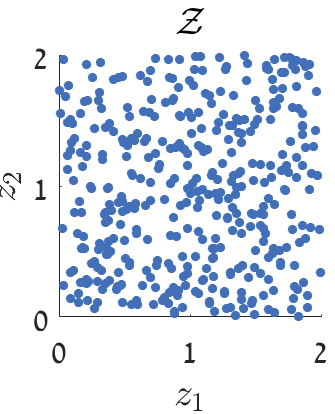
(a)

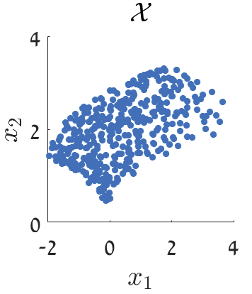
(b)

Figure 1: (a) The hidden random variables $\mathcal{Z}=\left\{\boldsymbol{z}_{i}\right\}_{i=1}^{N}$. (b) The observations $\mathcal{X}=\left\{\boldsymbol{x}_{i}\right\}_{i=1}^{N}$.

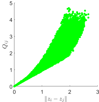
(a)

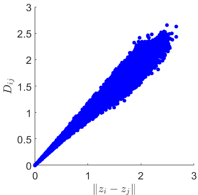
(b)

Figure 2: Comparison of Euclidean metric estimation. (a) The metric estimation based on [33]. (b) The metric estimation based on the middle point (16).

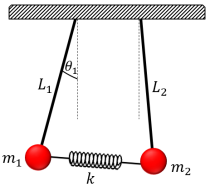
Figure 3: Illustration of the setup of the coupled pendulums system.

VII-B Coupled Pendulum

this experiment we simulate a coupled pendulum model. This model consists of two simple pendulums with lengths $L_{1}$ and $L_{2}$ and masses $m_{1}$ and $m_{2}$, which are connected by a spring as shown in Figure 3. For simplicity we set the same length and the same mass for both pendulums, namely $L_{1}=L_{2}=L$ and $m_{1}=m_{2}=m$. Let $u^{(i)}\left(t\right)$ and $w^{(i)}\left(t\right)$ denote the horizontal position and vertical position of the $i$th pendulum, respectively. Note that a close-form expression for the positions cannot be derived for the general case. Yet, in the case of small perturbations around the equilibrium point, we can consider a linear regime. Accordingly, let $\theta^{(i)}(t)=\arctan\left(u^{(i)}(t)/w^{(i)}(t)\right)$ be the angle between the $i$th pendulum and the vertical axis, and assume that $w^{(1)}\left(t\right)=w^{(2)}\left(t\right)=-L$, and $\sin\left(\theta^{(i)}\right)\approx\theta^{(i)}$. The ordinary differential equation (ODE) representing the horizontal position under the linear regime is given by:

$$\begin{cases}m\ddot{u}^{(1)}=-\frac{mg}{L}u^{(1)}-k\left(u^{(2)}-u^{(1)}\right)\\ m\ddot{u}^{(2)}=-\frac{mg}{L}u^{(2)}+k\left(u^{(2)}-u^{(1)}\right)\end{cases}$$ (19)

where $\ddot{u}$ is the second derivative of $u$, $g$ is the gravity of earth, and $k$ is the spring constant. For the following initial conditions:

$$\dot{u}_{1}\left(0\right)=0,u_{1}\left(0\right)=\delta,\dot{u}_{2}\left(0\right)=0,u_{2}\left(0\right)=0$$

where $0<\delta\in\mathbb{R}$ is assumed to be sufficiently small to satisfy the linear regime, the closed-form solution of the ODE (19) is given by:

$$\begin{cases}u^{(1)}\left(t\right)=\frac{1}{2}\delta\cos\left(\omega_{1}t\right)+\frac{1}{2}\delta\cos\left(\omega_{2}t\right)\\ u^{(2)}\left(t\right)=\frac{1}{2}\delta\cos\left(\omega_{1}t\right)-\frac{1}{2}\delta\cos\left(\omega_{2}t\right)\end{cases}$$ (20)

where

$$\omega_{1}=\sqrt{\frac{g}{L}},\ \ \omega_{2}=\sqrt{\frac{g}{L}+\frac{2k}{m}}$$

This example suits our purposes, since the horizontal displacement of each pendulum $u^{(i)}\left(t\right)$ is a linear combination of two harmonic motions with the common frequencies $\omega_{1}$ and $\omega_{2}$. In other words, the horizontal displacement of each pendulum can be viewed as a different observation of the same common harmonic motion.

To further demonstrate the power of our method, we assume that we do not have direct access to the horizontal displacement. Instead, we generate movies of the motion of the coupled pendulum in the linear regime. Consequently, on the one hand, we have a definitive ground truth described by the solution of the ODE of the system (the harmonic motion with the two frequencies $\omega_{1}$ and $\omega_{2}$). On the other hand, we only have access to high-dimensional nonlinear observations of the system, and we do not assume any prior model knowledge. Three snapshots of the entire system are displayed in Figure 4.

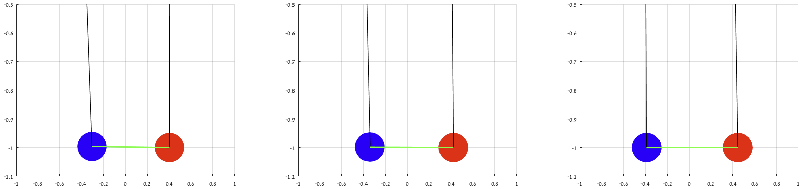
Figure 4: An example of $3$ snapshots of the coupled pendulum system.

This model is used to test our method in two scenarios. In the first scenario, we generate two movies of the two pendulums without any other features. In the second scenario, we generate two movies of the two pendulums, where each movie also contains an additional pendulum that represents an observation-specific geometric noise.

VII-B1 Case I – Coupled pendulum

We generate two movies, each is $5$ seconds long with $N=400$ frames (namely, sampling interval of $T_{s}=0.0125s$) of each of the pendulums in the couple pendulum system oscillating in a linear regime as demonstrated in Figure 5.

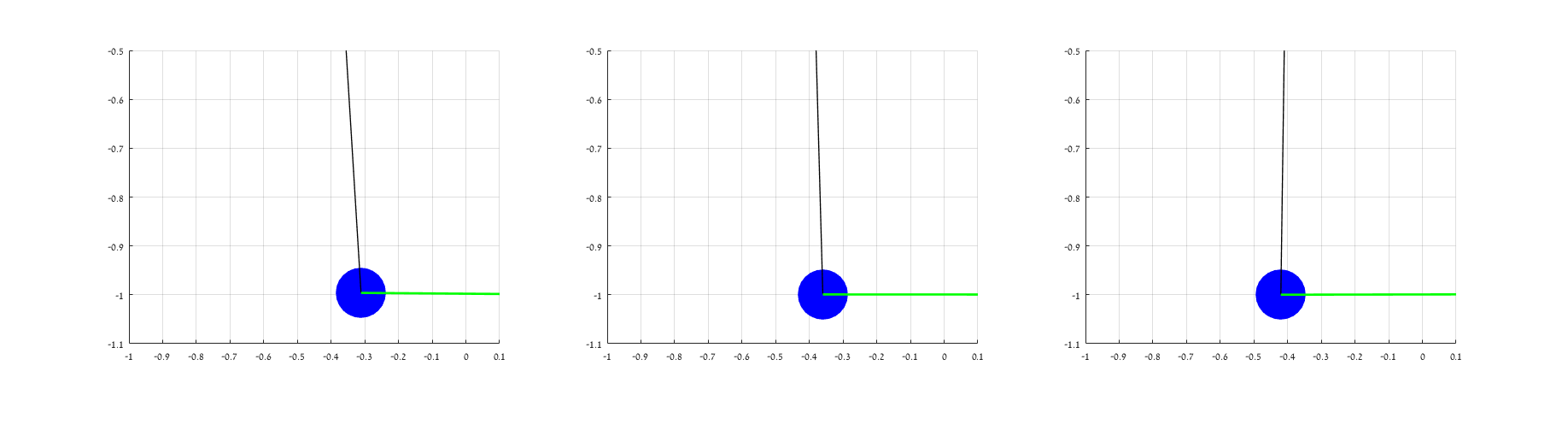
(a)

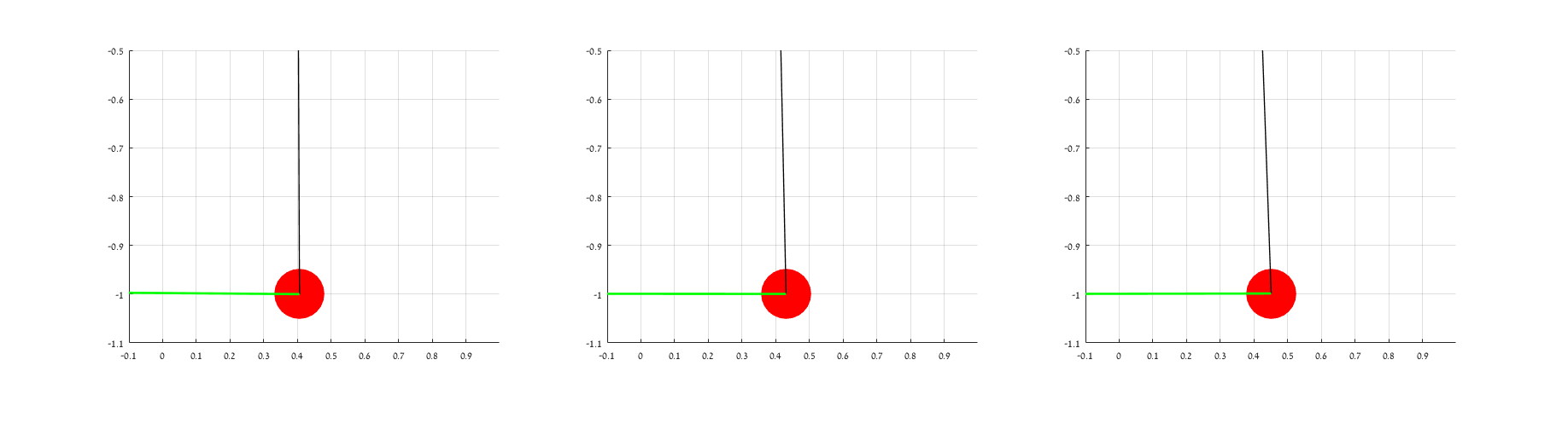
(b)

Figure 5: An example of $3$ frames of the each movie: (a) the left pendulum, and (b) the right pendulum.

Let $\boldsymbol{m}_{i}^{\left(1\right)}\in\mathbb{R}^{800}$ and $\boldsymbol{m}_{i}^{\left(2\right)}\in\mathbb{R}^{800}$ be two column stack vectors consisting of the pixels of the ith frame of the movies of the left and right pendulums, respectively. Let $\mathcal{X}=\left\{\boldsymbol{x}_{i}\right\}_{i=1}^{N}$ and $\mathcal{Y}=\left\{\boldsymbol{y}_{i}\right\}_{i=1}^{N}$ be two sets of observations, which are random projections of the frames of the movies. In the words, each observation is given by $\boldsymbol{x}_{i}=\boldsymbol{F}\boldsymbol{m}_{i}^{\left(1\right)}$ and $\boldsymbol{y}_{i}=\boldsymbol{G}\boldsymbol{m}_{i}^{\left(2\right)}$, where $\boldsymbol{F}\in\mathbb{R}^{200\times 800}$ and $\boldsymbol{G}\in\mathbb{R}^{200\times 800}$ are two fixed matrices with (approximately) orthonormal columns, drawn independently (once) from a Gaussian distribution. These observations/projections represent two different modalities in two different spaces.

We apply Algorithm 2 to $\mathcal{X}$ and $\mathcal{Y}$, where we use $8$ adjacent projected frames (in time), i.e., $\mathcal{X}_{i}=\left\{\boldsymbol{x}_{j}\right\}_{j=i-3}^{i+4}$ and $\mathcal{Y}_{i}=\left\{\boldsymbol{y}_{j}\right\}_{j=i-3}^{i+4}$, as the subset of each observation.

We compare our method to $3$ different algorithms: (i) Diffusion Maps with Euclidean metric (using only $\mathcal{X}$), (ii) KCCA, and (iii) Alternating Diffusion Maps (with Euclidean metric) [12]. In all four algorithms, we view the nontrivial eigenvector associated with the largest eigenvalue as the parametrization of the system, and we display its Fourier transform in Figure 6. In each subfigure the blue line is the Fourier transform of the eigenvector and the two vertical red dashed lines are the two frequencies of the coupled pendulum system: $\omega_{1}$ and $\omega_{2}$. Figure 6(a) displays the output of Diffusion Maps with the Euclidean metric using the set of observations $\mathcal{X}$ from only one movie. Figure 6(b) displays the output of KCCA. Figure 6(c) displays the output of Alternating Diffusion Maps. Finally, Figure 6(d) displays the output of Algorithm 2, i.e., Diffusion Maps with $D_{ij}$ (13) as its metric. We note that only one nontrivial eigenvector is presented, since, as shown in (20), the displacement of each pendulum, and hence, the projected frames of each movie, can be represented by a single scalar $\theta$, which is the angle of the pendulum with respect to the equilibrium axis. In other words, the coupled pendulum system can be described using a low-dimensional representation conveyed by the dominant nontrivial eigenvector.

As we can see in Figure 6, both in the result obtained by Diffusion Maps as well as in the result obtained by our method, the presented eigenvector contains the frequencies of the coupled pendulum system: $\omega_{1}$ and $\omega_{2}$. In contrast, the eigenvector attained by Alternating Diffusion Maps and the eigenvector attained by KCCA do not contain the true frequencies of the coupled pendulum system. Specifically, we show in Figure 6(a) that the true frequencies can be extracted simply by applying diffusion maps to one of the observation sets. Consequently, we remark that this experiment serves only as a reference; it implies that in this noiseless case each of the sets carries the full information on the system, and as a result, these frequencies are common to both sets. In the next section, we introduce noise and show that in the noisy case our algorithm is essential.

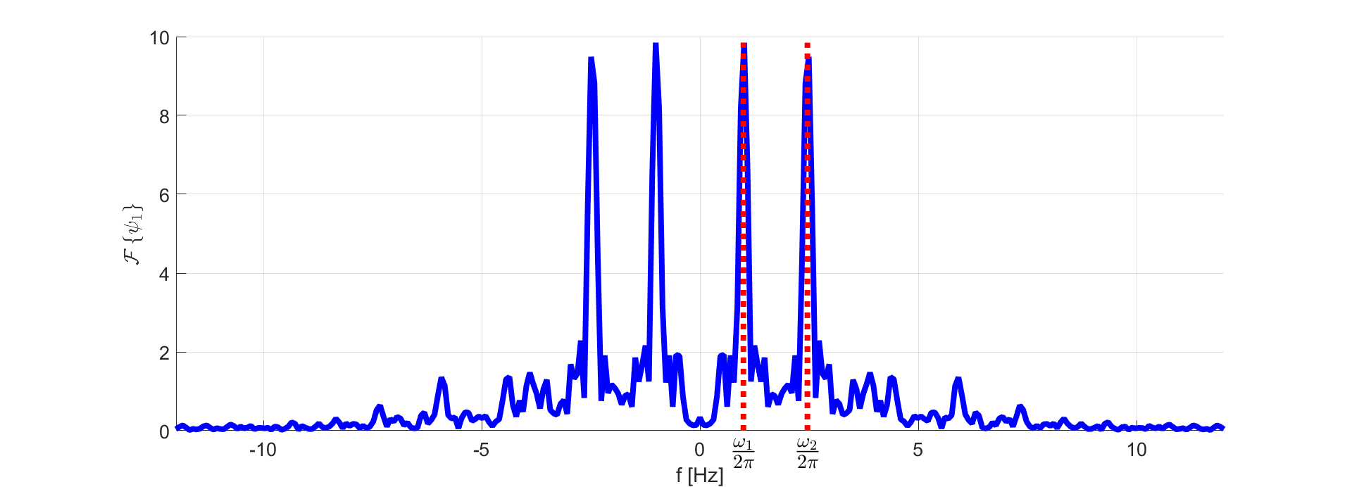
(a)

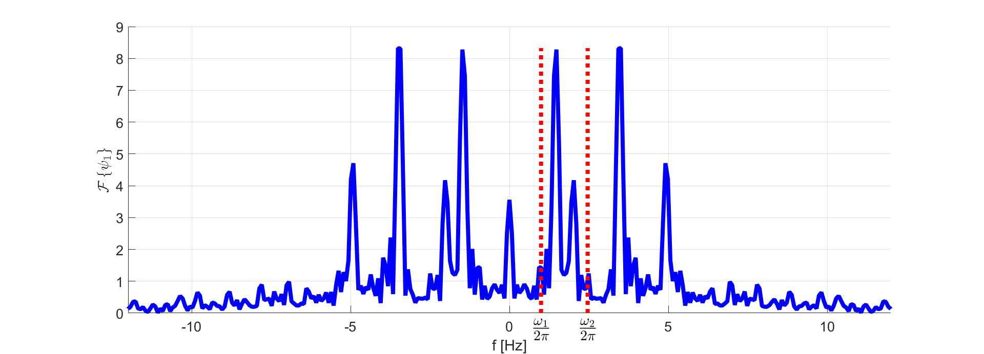
(b)

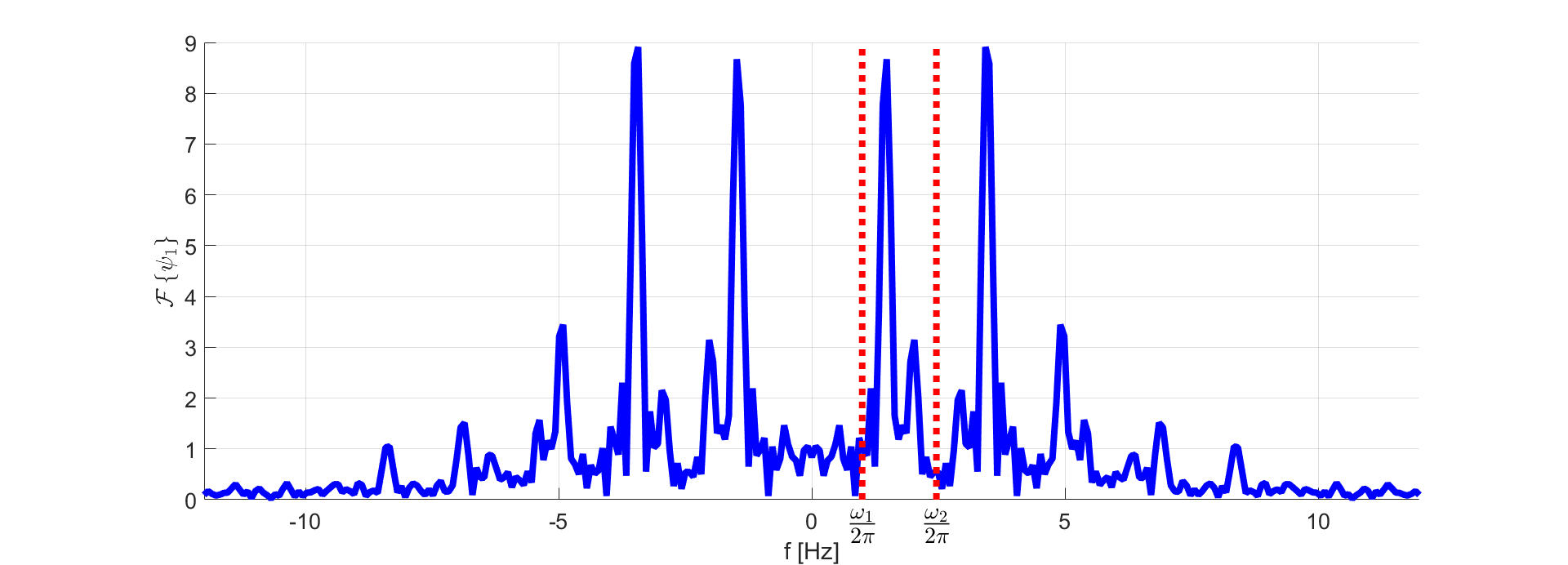
(c)

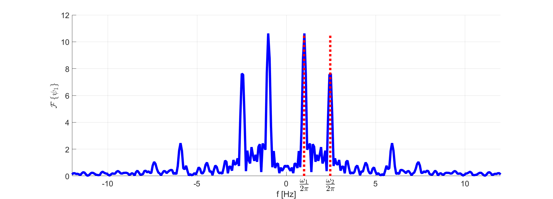
(d)

Figure 6: The Fourier transform of the dominant eigenvectors attained by: (a) Diffusion Maps based on a single set $\mathcal{X}$, (b) KCCA, (c) Alternating Diffusion Maps, and (d) Algorithm 2. The blue curves are the Fourier transforms of the eigenvectors and the vertical dashed lines represent the two frequencies of the system $\omega_{1}$ and $\omega_{2}$.

VII-B2 Case II – Coupled pendulum with observation-specific noise

We repeat the experiment described in Section VII-B1 with additional observation-specific noise. In this experiment, an additional simple pendulum is added to each movie as demonstrated in Figure 7. Note that the two extra pendulums, one in each movie, oscillate in different frequencies: $\omega_{3}=\frac{1}{5}\omega_{1}$ and $\omega_{4}=4\omega_{1}$. In other words, we now have $4$ different frequencies in the movies, yet only $2$ of them ($\omega_{1}$ and $\omega_{2}$) are common to both observations.

We apply Algorithm 2 with the same selection of subsets $\mathcal{X}_{i}$ and $\mathcal{Y}_{i}$. As in Section VII-B1, we compare our method to the same 3 algorithms.

Figure 8 is similar to Figure 6, where we display the Fourier transforms of the eigenvectors obtained by the algorithms. In each subfigure the blue curve is the Fourier transform of the eigenvector, the two red dashed vertical lines are the two frequencies of the coupled pendulum $\omega_{1}$ and $\omega_{2}$, and the two green dashed vertical lines are the two frequencies of the simple pendulums $\omega_{3}$ and $\omega_{4}$. Figure 8(a) displays the output of Diffusion Maps with the Euclidean metric using frames from only one movie $\mathcal{X}$. Figure 8(b) displays the output of KCCA. Figure 8(c) displays the output of Alternating Diffusion Maps. Finally, Figure 8(d) displays the output of Algorithm 2, i.e., Diffusion Maps with the metric $D_{ij}$.

As we can see in Figure 8, only in the result obtained Algorithm 2, the dominant eigenvector contains the frequencies of the coupled pendulum system $\omega_{1}$ and $\omega_{2}$ as desired. The eigenvectors attained by Diffusion Maps, by KCAA, and by Alternating Diffusion Maps do not contain the true frequencies of the coupled pendulum system.

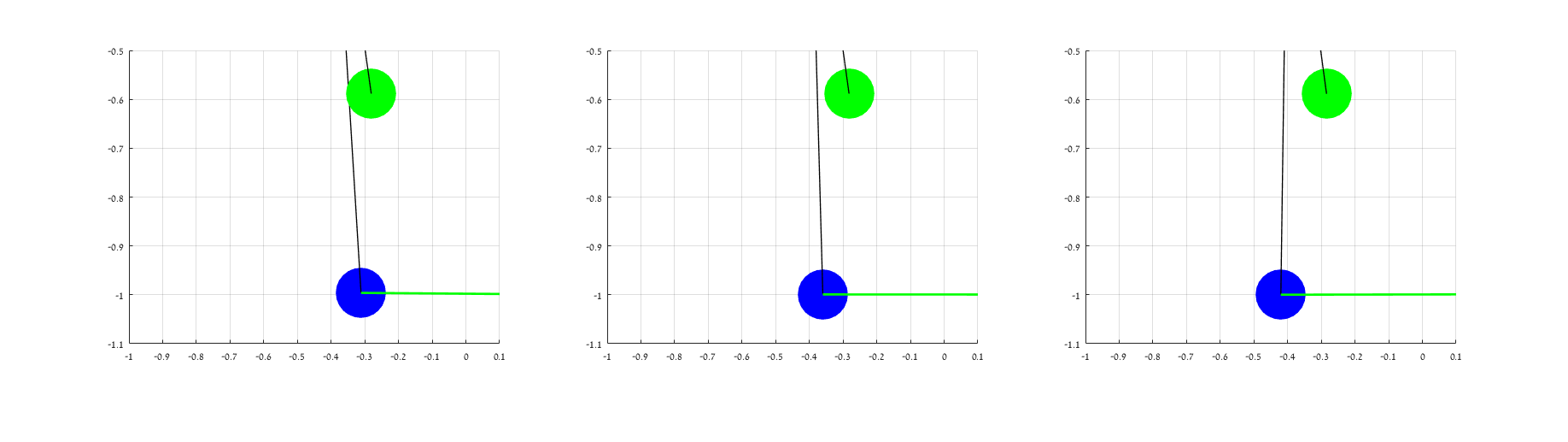
(a)

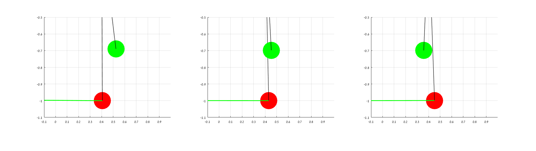
(b)

Figure 7: An example of $3$ frames of the noisy movie. (a) The left movie which captures the left coupled pendulum (blue) and an additional simple pendulum (green). (b) The right movie which captures the right coupled pendulum (red) and an additional simple pendulum (green).

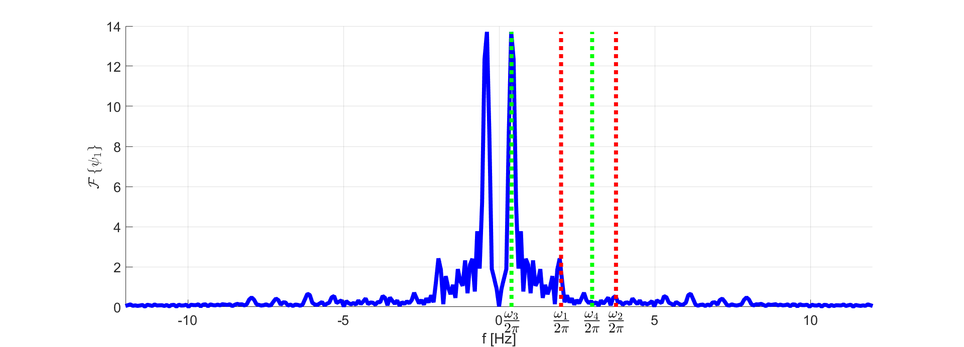
(a)

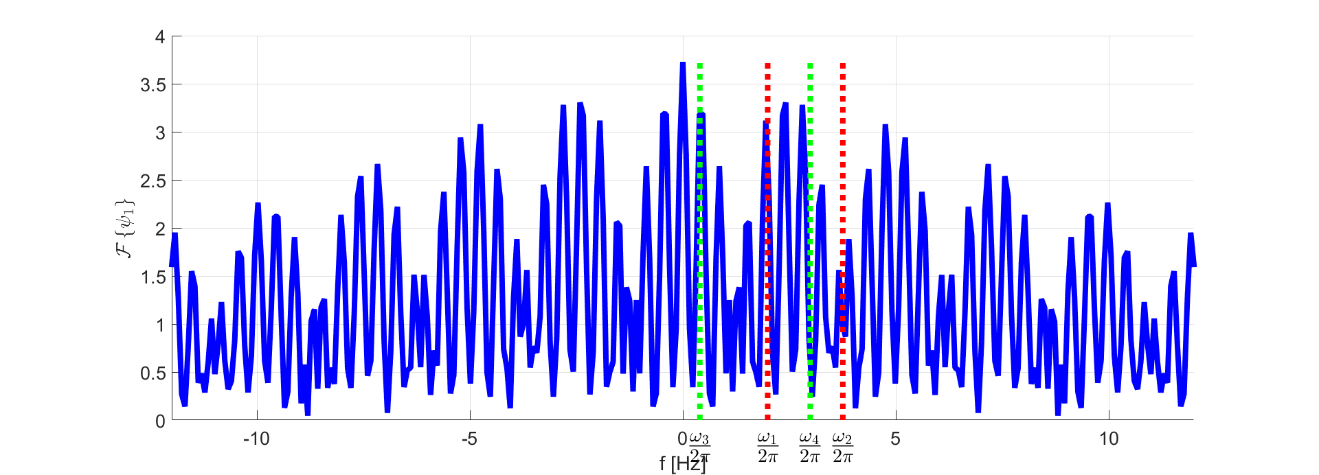
(b)

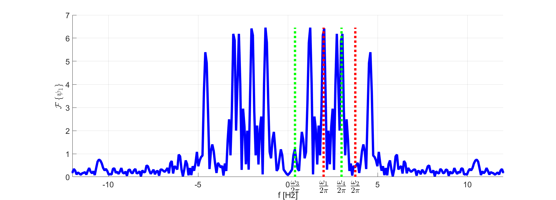
(c)

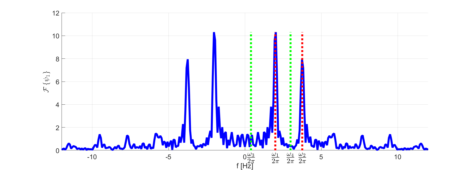
(d)

Figure 8: The output of the $4$ algorithms applied to the coupled pendulum movies with additional noise: (a) Diffusion Maps, (b) KCCA, (c) Alternating Diffusion Maps, and (d) Algorithm 2. The Fourier transforms of the dominant non-trivial eigenvectors are displayed as blue curves. The red and green dashed vertical lines represent the frequencies of the coupled pendulum and the simple uncoupled pendulum, respectively.

VII-C Multiple Observations of Rotating Icons

In this simulation we show that Algorithm 4 allows for the accurate parametrization of the common variable underlying $K=3$ nonlinear high-dimensional observations. We generate three high-dimensional movies containing four rotating icons: Super Mario, Mushroom, Turtle and Flower. Each movie captures only two icons. In the movies, each icon rotates in a constant angular speed: the angular speeds of Super Mario, Mushroom, Turtle and Flower are $4^{\circ}$,$6^{\circ}$,$10^{\circ}$, and $15^{\circ}$ per frame, respectively, as demonstrated in Figure 9. Notice that only Mushroom appears in all the movies, and hence, the angular speed of Mushroom is the hidden common variable $z$, whereas the angular speeds of the other icons are the hidden observation-specific variables $\epsilon^{\left(k\right)}$, for $1\leq k\leq K$. Two frames of each movie are depicted for illustration in Figure 9.

(a)

(b)

(c)

(d)

(e)

(f)

Figure 9: Two frames of each of the movies: (a) and (d) are from the first movie, (b) and (e) from the second movie, and (c) and (f) from the third movie. Mushroom is common to all the movies while the other icons are specific for each movie.

Each set of nonlinear high-dimensional observations $\mathcal{X}^{\left(k\right)}=\left\{\boldsymbol{x}_{i}^{\left(k\right)}\right\}_{i=1}^{N}$ consists of $N=300$ frames. We apply Algorithm 4, where in step 1(a), the subsets $\mathcal{X}_{i}^{\left(k\right)}$ consist of the frames in a time window of length $7$ around $\boldsymbol{x}_{i}^{\left(k\right)}$. Since, the desired parametrization should convey the fact that the common variable in the sets is the angular speed of Mushroom, and thus, it should be periodic with the same period, we apply the Fourier transform to the first column of $\boldsymbol{\Psi}$ and present it in Figure 10. In Figure 10, the true frequencies of Super Mario, Mushroom, Turtle and Flower are marked by vertical red, green, black and pink dashed lines, respectively.

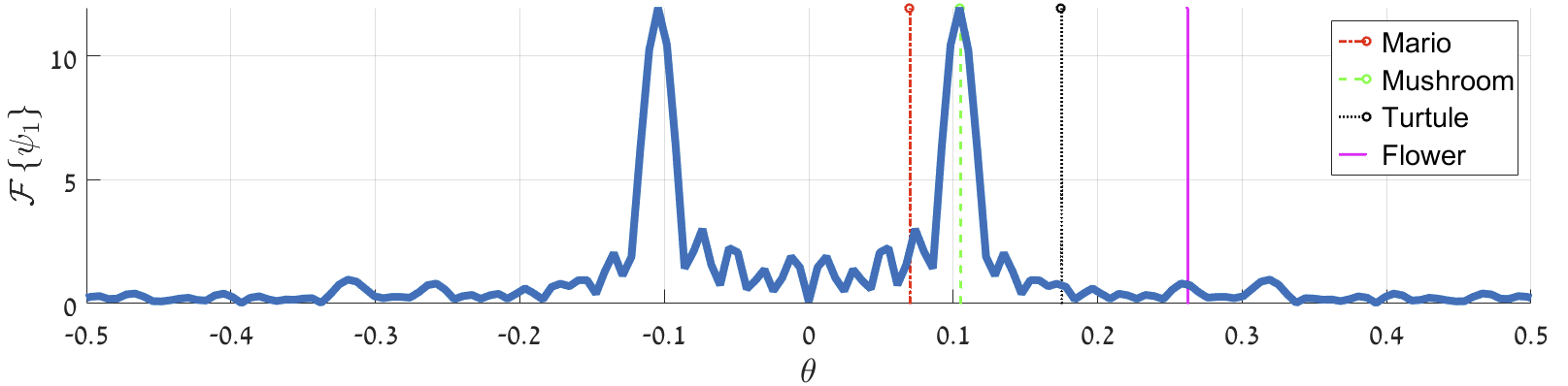
Figure 10: The Fourier transform of the parametrization of the common variable obtained by Algorithm 4. The vertical dashed lines represent the true frequencies of the rotating icons.

Figure 10 shows that indeed the proposed algorithm identifies the frequency of Mushroom (the common variable underlying all observation sets), whereas the frequencies of the observation-specific Super Mario, Turtle and Flower are completely missing, as expected.

To further demonstrate the capabilities of our method, we repeat the simulation in a more complex setting. Here, each pair of movies contains two common icons while only Mushroom is maintained as the common variable of all the movies. Two frames of the new movies are depicted for illustration in Figure 11.

(a)

(b)

(c)

(d)

(e)

(f)

Figure 11: Two frames from each movie: (a) and (d) are from the first movie, (b) and (e) from the second movie, and (c) and (f) from the third movie. Each two movies contain two common icons. Only Mushroom is common to all the movies.

For similar reasons as in the previous experiment, we apply the Fourier transform to the first column of $\boldsymbol{\Psi}$ and present it in Figure 12. In Figure 12, the true frequencies of Super Mario, Mushroom, Turtle and Flower are marked by vertical dashed red, green, black and pink lines, respectively. Despite the more complex setting, in which any two observation sets contain additional correlated “noise”, Figure 12 shows that the proposed algorithm identifies the true frequency of the common variable (Mushroom).

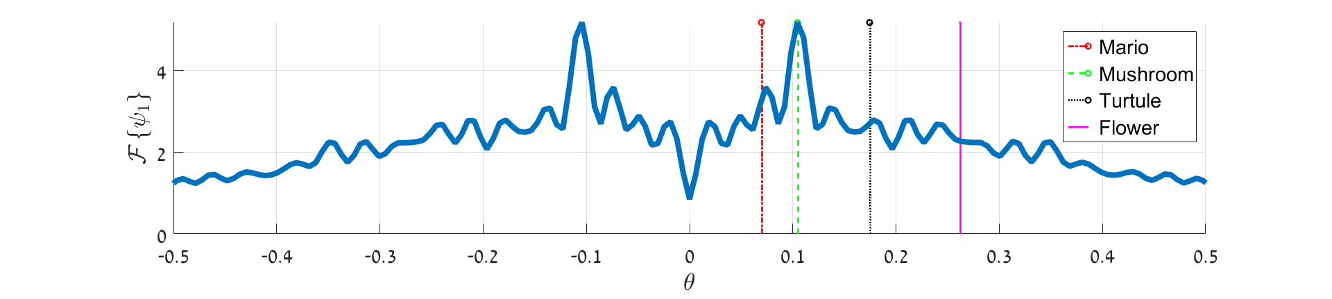
Figure 12: The Fourier transform of the parametrization of the common variable obtained by Algorithm 4. The vertical dashed lines represent the true frequencies of the rotating icons.

In summary, in this simulation without assuming any prior knowledge on the structure and content of the data, our extended method successfully discovers the common variable hidden in multiple high-dimensional and nonlinear observations.

VIII Conclusions

In this paper, we have presented a new manifold learning method for extracting the common hidden variables underlying multimodal data sets. Our method does not assume prior knowledge on the system nor on the observed data and relies on a local metric, which is learned from data in an unsupervised manner. Specifically, we proposed a metric between observations based on local CCA and showed that this metric approximates the Euclidean distance between the respective hidden common variables.

The theoretical results were validated in simulations, where we demonstrated the accurate recovery of the hidden common variables from multiple complex and high-dimensional data sets. In addition, we showed that our method can be applied to various different types of observations and attain the same results without adjusting the algorithm to the specific observations at hand. For example, the coupled pendulum system is an example of a dynamical system with a definitive model and a closed-form solution in the linear case. We have shown that without any prior model knowledge our method can obtain an accurate description of the solution solely from high-dimensional nonlinear observations. Note that our solution was obtained also when the observations contained “structured noise”.

The capability to obtain the close-form solution solely from observations enables us to demonstrate the power of our approach by carrying out empirical modeling of dynamical systems. One can further extend this to the analysis of the coupled pendulum system in more complex scenarios, such as, with different initial conditions and in nonlinear regimes. In such cases, closed-form solutions may no longer be available. Yet, from a data-driven point of view, our method is expected to attain an accurate description of the system from its observations. Importantly, since our method does not require prior rigid model assumptions, it can be applied to a broad variety of multimodal data sets lacking definitive models. Therefore, future work will address the extension of our analysis to various types of dynamical systems and empirical physics experiments.

References

- [1] D. Lahat, T. Adali, and C. Jutten, “Multimodal data fusion: an overview of methods, challenges, and prospects,” Proc. IEEE, vol. 103, no. 9, pp. 1449–1477, 2015.
- [2] H. Hotelling, “Relations Between Two Sets of Variates,” Biometrika, vol. 28, no. 3/4, pp. 321–377, Dec. 1936.
- [3] D. R. Hardoon, S. Szedmak, and J. Shawe-Taylor, “Canonical correlation analysis: An overview with application to learning methods,” Neural computation, vol. 16, no. 12, pp. 2639–2664, 2004.
- [4] F. R. Bach and M. I. Jordan, “A probabilistic interpretation of canonical correlation analysis,” 2005.
- [5] P. L. Lai and C. Fyfe, “Kernel and nonlinear canonical correlation analysis,” International Journal of Neural Systems, vol. 10, no. 5, pp. 365–377, 2000.
- [6] Wenming Zheng, Xiaoyan Zhou, Cairong Zou, and Li Zhao, “Facial expression recognition using kernel canonical correlation analysis (kcca),” Neural Networks, IEEE Transactions on, vol. 17, no. 1, pp. 233–238, 2006.
- [7] Thomas Melzer, Michael Reiter, and Horst Bischof, “Appearance models based on kernel canonical correlation analysis,” Pattern recognition, vol. 36, no. 9, pp. 1961–1971, 2003.
- [8] David R Hardoon, Janaina Mourao-Miranda, Michael Brammer, and John Shawe-Taylor, “Unsupervised analysis of fmri data using kernel canonical correlation,” NeuroImage, vol. 37, no. 4, pp. 1250–1259, 2007.
- [9] V. R. de Sa, “Spectral clustering with two views,” in ICML workshop on learning with multiple views, 2005, pp. 20–27.
- [10] Bo Wang, Jiayan Jiang, Wei Wang, Zhi-Hua Zhou, and Zhuowen Tu, “Unsupervised metric fusion by cross diffusion,” in Computer Vision and Pattern Recognition (CVPR), 2012 IEEE Conference on. IEEE, 2012, pp. 2997–3004.
- [11] B. Boots and G. Gordon, “Two-manifold problems with applications to nonlinear system identification,” in ICML, 2012.
- [12] R. R. Lederman and R. Talmon, “Learning the geometry of common latent variables using alternating-diffusion,” Appl. Comput. Harmon. Anal., 2015.
- [13] Roy R Lederman, Ronen Talmon, Hau-Tieng Wu, Yu-Lun Lo, and Ronald R Coifman, “Alternating diffusion for common manifold learning with application to sleep stage assessment,” in Acoustics, Speech and Signal Processing (ICASSP), 2015 IEEE International Conference on. IEEE, 2015, pp. 5758–5762.
- [14] S. T. Roweis and L. K. Saul, “Nonlinear dimensionality reduction by locally linear embedding,” Science, vol. 290, no. 5500, pp. 2323–2326, 2000.
- [15] M. Belkin and P. Niyogi, “Laplacian eigenmaps for dimensionality reduction and data representation,” Neural computation, vol. 15, no. 6, pp. 1373–1396, 2003.
- [16] R. R. Coifman and S. Lafon, “Diffusion maps,” Appl. Comput. Harmon. Anal., vol. 21, no. 1, pp. 5–30, 2006.
- [17] A. Singer and R. R. Coifman, “Non-linear independent component analysis with diffusion maps,” Appl. Comput. Harmon. Anal., vol. 25, no. 2, pp. 226 – 239, 2008.
- [18] R. Talmon and R. R. Coifman, “Empirical intrinsic geometry for nonlinear modeling and time series filtering,” Proceedings of the National Academy of Sciences, vol. 110, no. 31, pp. 12535–12540, 2013.
- [19] R. Talmon and R. R. Coifman, “Intrinsic modeling of stochastic dynamical systems using empirical geometry,” Appl. Comput. Harmon. Anal., vol. 39, no. 1, pp. 138 – 160, 2015.
- [20] Ronen Talmon, Stéphane Mallat, Hitten Zaveri, and Ronald R Coifman, “Manifold learning for latent variable inference in dynamical systems,” Signal Processing, IEEE Transactions on, vol. 63, no. 15, pp. 3843–3856, 2015.
- [21] T. Berry and T. Sauer, “Local kernels and the geometric structure of data,” Appl. Comput. Harmon. Anal., 2015.
- [22] Dimitrios Giannakis, “Dynamics-adapted cone kernels,” SIAM Journal on Applied Dynamical Systems, vol. 14, no. 2, pp. 556–608, 2015.
- [23] Virginia R De Sa, Patrick W Gallagher, Joshua M Lewis, and Vicente L Malave, “Multi-view kernel construction,” Machine learning, vol. 79, no. 1-2, pp. 47–71, 2010.
- [24] Abhishek Kumar, Piyush Rai, and Hal Daume, “Co-regularized multi-view spectral clustering,” in Advances in Neural Information Processing Systems, 2011, pp. 1413–1421.
- [25] Yen Yu Lin, Tyng Luh Liu, and Chiou Shann Fuh, “Multiple kernel learning for dimensionality reduction,” Pattern Analysis and Machine Intelligence, IEEE Transactions on, vol. 33, no. 6, pp. 1147–1160, 2011.
- [26] Hsin-Chien Huang, Yung-Yu Chuang, and Chu-Song Chen, “Affinity aggregation for spectral clustering,” in Computer Vision and Pattern Recognition (CVPR), 2012 IEEE Conference on. IEEE, 2012, pp. 773–780.
- [27] Byron Boots and Geoff Gordon, “Two-manifold problems with applications to nonlinear system identification,” arXiv preprint arXiv:1206.4648, 2012.
- [28] Ofir Lindenbaum, Arie Yeredor, Moshe Salhov, and Amir Averbuch, “Multiview diffusion maps,” arXiv preprint arXiv:1508.05550, 2015.
- [29] Ofir Lindenbaum, Arie Yeredor, and Moshe Salhov, “Learning coupled embedding using multiview diffusion maps,” in Latent Variable Analysis and Signal Separation, pp. 127–134. Springer, 2015.
- [30] Tomer Michaeli, Weiran Wang, and Karen Livescu, “Nonparametric canonical correlation analysis,” arXiv preprint arXiv:1511.04839, 2015.
- [31] Yong Luo, Dacheng Tao, Kotagiri Ramamohanarao, Chao Xu, and Yonggang Wen, “Tensor canonical correlation analysis for multi-view dimension reduction,” Knowledge and Data Engineering, IEEE Transactions on, vol. 27, no. 11, pp. 3111–3124, 2015.
- [32] Lieven De Lathauwer, Bart De Moor, and Joos Vandewalle, “A multilinear singular value decomposition,” SIAM journal on Matrix Analysis and Applications, vol. 21, no. 4, pp. 1253–1278, 2000.
- [33] O. Yair and R. Talmon, “Multimodal metric learning with local CCA,” submitted, 2016.
- [34] Dan Kushnir, Ali Haddad, and Ronald R Coifman, “Anisotropic diffusion on sub-manifolds with application to earth structure classification,” Applied and Computational Harmonic Analysis, vol. 32, no. 2, pp. 280–294, 2012.
- [35] L. M. Ewerbring and F. T. Luk, “Canonical correlations and generalized SVD: applications and new algorithms,” in 32nd Annual Technical Symposium, 1989, pp. 206–222.
- [36] Carmeline J Dsilva, Ronen Talmon, C William Gear, Ronald R Coifman, and Ioannis G Kevrekidis, “Data-driven reduction for multiscale stochastic dynamical systems,” arXiv preprint arXiv:1501.05195, 2015.
- [37] Pierre Comon, Xavier Luciani, and André LF De Almeida, “Tensor decompositions, alternating least squares and other tales,” Journal of Chemometrics, vol. 23, no. 7-8, pp. 393–405, 2009.