High spatial resolution Fe xii observations of solar active regions

Abstract

We use UV spectral observations of active regions with the Interface Region Imaging Spectrograph (IRIS) to investigate the properties of the coronal Fe xii 1349.4Å emission at unprecedented high spatial resolution ($\sim 0.33$ ^′′). We find that by using appropriate observational strategies (i.e., long exposures, lossless compression), Fe xii emission can be studied with IRIS at high spatial and spectral resolution, at least for high density plasma (e.g., post-flare loops, and active region moss). We find that upper transition region (moss) Fe xii emission shows very small average Doppler redshifts ($v_{\rm D}$ $\sim 3$ km s^-1), as well as modest non-thermal velocities (with an average $\sim 24$ km s^-1, and the peak of the distribution at $\sim 15$ km s^-1). The observed distribution of Doppler shifts appears to be compatible with advanced 3D radiative MHD simulations in which impulsive heating is concentrated at the transition region footpoints of a hot corona. While the non-thermal broadening of Fe xii 1349.4Å peaks at similar values as lower resolution simultaneous Hinode-EIS measurements of Fe xii 195Å, IRIS observations show a previously undetected tail of increased non-thermal broadening that might be suggestive of the presence of subarcsecond heating events. We find that IRIS and EIS non-thermal line broadening measurements are affected by instrumental effects that can only be removed through careful analysis. Our results also reveal an unexplained discrepancy between observed 195.1/1349.4Å Fe xii intensity ratios and those predicted by the CHIANTI atomic database.

1. Introduction

The nature and properties of the heating of the outer atmosphere of the Sun and solar-like stars to millions of degrees are issues that remain largely unsolved (e.g., reviews by Klimchuk, 2006; Testa et al., 2015). The complex problem of coronal heating is addressed by constraining models through observational determinations of the plasma conditions (temperature, density, flows, and their spatial and temporal distribution throughout the atmosphere) in solar and stellar coronae. Solar observations are a particularly powerful tool to investigate the heating processes, because they provide high spatial and temporal resolution, for both imaging and spectroscopic data, and significant progress has been recently made. Two main candidate heating mechanisms have been studied and modeled in some detail: dissipation of magnetohydrodynamic (Alfv$\acute{\rm e}$n) waves (e.g., van Ballegooijen et al., 2011, 2014), and dissipation of magnetic stresses in small scale reconnection events (“nanoflares”), due to random photospheric motions that lead to braiding of magnetic field lines (e.g., Parker, 1988; Galsgaard & Nordlund, 1996; Cargill, 1996; Priest et al., 2002; Gudiksen & Nordlund, 2005; Hansteen et al., 2015).

Observational diagnostics of coronal heating are however often difficult to achieve because of the typically very small (compared to current resolution capabilities) spatial and temporal scales of heating release predicted by most viable heating processes (e.g., Klimchuk, 2006; Reale, 2014). Furthermore, the immediate plasma response to impulsive heating events is challenging to detect because of several effects, including non-equilibrium ionization and the low emission measure causing a very faint emission from the hot plasma (e.g., Reale, 2014; Testa et al., 2011). In flares the heated plasma is dense and bright, allowing the study of the heating processes, but in the non-flaring corona the detectability of the heated plasma is a significant challenge. For the non-flaring corona, the study of the transition region emission provides a powerful alternative approach to the study of coronal heating as it overcomes several issues present in coronal observations: the emission of the dense transition region is (a) bright, (b) confined to a small atmospheric layer (compared to the large coronal volumes) therefore dramatically reducing the line of sight overlap of a different structures, (c) very sensitive to heating events. For these reasons, in this paper we mostly focus on this transition region emission, and in particular on “moss”, i.e., the upper transition region (TR) layer at the footpoints of high pressure loops in active regions, which is very bright in observations sensitive to $\sim 1$ MK emission (e.g., Peres et al., 1994; Fletcher & De Pontieu, 1999; Berger et al., 1999; De Pontieu et al., 1999; Martens et al., 2000; Brooks et al., 2009; Tripathi et al., 2010; Winebarger et al., 2013; Testa et al., 2013, 2014).

In this paper we focus on spectral observations, which provide particularly useful constraints on coronal heating models. The spectral line profiles (Doppler shifts, and line broadening) of coronal and transition region emission diagnose plasma motions (e.g., flows and turbulence) that can be compared with expectations from model. For instance, significant non-thermal line broadening (i.e., broadening in excess of the thermal and instrumental broadening), is predicted by several reconnection based models (e.g., Cargill, 1996; Patsourakos & Klimchuk, 2006) and Alfv$\acute{\rm e}$n wave models (e.g., van Ballegooijen et al., 2011; Asgari-Targhi et al., 2014). Impulsive heating models predict a range of Doppler shifts (e.g., Patsourakos & Klimchuk, 2006; Hansteen et al., 2010; Taroyan & Bradshaw, 2014) depending on the details of the model (e.g., spatial and temporal distribution of heating) as discussed in more detail in § 5.

Non-thermal line broadening and Doppler shifts in plasma in the solar outer atmosphere have been studied since the Skylab era (e.g., Doschek et al., 1976; Doschek & Feldman, 1977; Doschek et al., 1981) in a variety of chromospheric, transition region, and coronal spectral lines. In the following decades, the Ultraviolet Spectrometer on the Solar Maximum Mission (Woodgate et al., 1980), the NRL High Resolution Telescope and Spectrograph (HRTS; Bartoe 1982), the Solar Ultraviolet Measurements of Emitted Radiation spectrometer (SUMER; Wilhelm et al. 1995) onboard SOHO, and the Extreme-ultraviolet Imaging Spectrometer (EIS; Culhane et al. 2007) onboard Hinode (Kosugi et al., 2007) have provided spectral observations with improved spatial and spectral resolution. Measurements before EIS however mostly focused on transition region lines formed below $\sim 1$ MK, and/or on quiet sun or coronal holes (e.g., Athay et al., 1983; Dere et al., 1984; Warren et al., 1997; Chae et al., 1998a, b; Akiyama et al., 2005). Early spectroscopic active region observations of emission lines formed around $\sim 1$ MK in a variety of solar coronal features (quiet Sun and active regions, including both on disk and off-limb observations) indicated that the non-thermal width ($w_{\rm nth}$) was characterized by relatively small $w_{\rm nth}$ ($\sim 10-25$ km s^-1; e.g., Cheng et al. 1979). Fewer early studies investigated the Doppler shifts of coronal lines (more uncertain than line broadening due to their dependence on the accuracy of rest wavelength and of absolute wavelength calibration) and the results pointed to a range of values from small blueshifts (e.g., Sandlin et al., 1977) to small redshifts ($\lesssim 10$ km s^-1; Dere 1982, e.g.,; Achour et al. 1995, e.g.,), to relatively large redshifts ($10-30$ km s^-1; Brueckner 1981). Several recent studies based on EIS spectra have helped better determine the spectral line properties of coronal emission lines in active regions. Brooks et al. (2009) studied Doppler shifts and non-thermal velocities in active region moss using the EIS Fe xii 195Å line, and find $w_{\rm nth}$ values in the 15-30 km s^-1 range, and Doppler shifts from $\sim-5$ km s^-1 (i.e., blueshifts) to $\sim 10$ km s^-1 (redshift). Tripathi et al. (2012) investigated Doppler shifts in moss emission and, using a different method than Brooks et al. (2009) for defining a reference wavelength, found for Fe xii a symmetric distribution ($-10-10$ km s^-1) centered around zero shift. Dadashi et al. (2012) using yet another calibration method for the wavelength, finds blueshifts in Fe xii with typical values of $-10$ to $-5$ km s^-1 in moss.

Here we present a first analysis of spectroscopic observations of Fe xii emission, obtained at unprecedented spatial resolution of $\sim 0.33$^′′ with the Interface Region Imaging Spectrograph (IRIS; De Pontieu et al. 2014). IRIS spatial resolution represents an improvement by a factor of at least 5 ($\sim 16$ IRIS pixel for each EIS pixel) with respect to previous spectrographs observing the chromosphere/transition region/corona in UV/EUV/X-ray spectral wavelengths. Also, as hinted by recent coronal studies (Warren et al., 2008; Testa et al., 2013; Peter et al., 2013; Antolin et al., 2015), the collective behavior in the corona is starting to be resolved at spatial scales of the order of $\sim 0.3$^′′. IRIS provides slit-jaw images (SJI) and high resolution spectra in the UV range, allowing to study the chromospheric and transition region emission at high resolution. The presence of chromospheric neutral lines in the IRIS spectra allows a much more accurate calibration of the absolute wavelength, compared with EIS. The IRIS FUV spectral range includes a Fe xii forbidden line at 1349.4Å (3s² 3p^{3 4}S_3/2 - 3s² 3p^{3 2}P_1/2). This coronal line (peak formation temperature around $\log T$[K]$\sim 6.2$) was observed with Skylab (e.g., Doschek & Feldman, 1977; Sandlin et al., 1977), together with a stronger forbidden line of Fe xii at 1242Å to provide also coronal density diagnostics (Cook et al., 1994, e.g.,). Both lines hower were too weak to be observed on disk and were generally detected with Skylab only in long exposure off-limb spectra (Feldman et al., 1983), and with very limited spatial resolution. These coronal forbidden lines were also observed by SUMER, but very few active region measurements (in the stronger 1242Å) are available (e.g., Teriaca et al., 1999; De Pontieu et al., 2009).

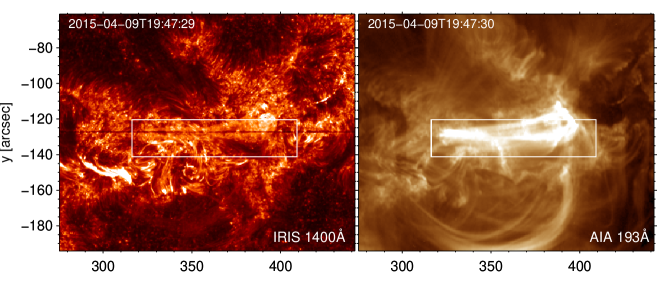
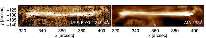
Figure 1.— IRIS and SDO-AIA observations of AR 12320. Top: IRIS slit-jaw image in the 1400Å passband (left), and AIA 193Å image (right). For a subregion, indicated by the box in the IRIS SJI and AIA images, we also show the intensity map in the Fe xii 1349Å line (from Gaussian fit to the IRIS spectra; bottom left), and the corresponding composite AIA 193Å image (built by selecting, for each horizontal slice of the IRIS field of view (f.o.v.) the AIA data closest in time; bottom right).

In this paper we show that the 1349Å Fe xii line, though weak, can be observed with IRIS at high spatial resolution, provided that long enough ($\sim 30$s) exposure times and appropriate observing modes are used (see § 2 for details). Here we analyze two datasets with bright targets, post-flare loops and active region moss, for which the Fe xii emission can be observed with IRIS at good signal-to-noise (see § 2). For the moss dataset we also present a detailed comparison with coordinated EIS observations, focusing in particular on the Fe xii 195Å emission. In section 2 we describe the data selection process and selected datasets, while in section 3 we address analysis methods and results. In section 4 we present the results of a 3D radiative MHD simulation we use as an aid for the interpretation of the observed spectral properties of the Fe xii moss emission. We discuss our findings and draw our conclusions in section 5.

2. Data Selection and Reduction

The goal of this work is to analyze Fe xii spectral properties for the first time at the high spatial resolution of IRIS observations. The Fe xii 1349.4Å forbidden line is characterized by very modest typical emission levels compared to the much stronger allowed Fe xii transitions at EUV wavelengths; e.g., the EIS Fe xii 195.12Å line, which we will analyze in this paper as well, has emission $\gtrsim 2$ orders of magnitude higher than the IRIS 1349.4Å line, according to predictions based on the CHIANTI atomic database (Dere et al., 1997; Landi et al., 2012; Del Zanna et al., 2015). Inspection of IRIS observations quickly shows that exposure times of the order of 30s are needed to obtain high enough signal-to-noise ratio (SNR) to analyze the Fe xii emission at the highest IRIS spatial resolution.

In this paper we present results for two IRIS active region datasets, which have relatively bright Fe xii emission. The first dataset, shown in Figure 1, is part of a series of observations we tailored to study the Fe xii emission in active regions. For the selected sequence IRIS observed AR 12320 (2015-04-09 19:24-20:31UT), with 64-step dense rasters (in “dense” rasters the raster step is 0.35^′′), 30s exposure times, $2\times 2$ spatial and spectral binning, lossless compression (IRIS OBSID 3810112091), and a roll angle of -90^∘ (i.e., the slit was oriented in the E-W direction). Slit-jaw images (SJI) were obtained at each raster position, alternating all four passbands (1330Å, 1400Å, 2796Å, 2832Å) therefore yielding a cadence of $\sim 125$s in each passband. In this dataset both the FUV and NUV spectra have $\Delta\lambda\sim 0.025$Å, and their field of view (f.o.v.) is $\sim 21$^′′$\times 175$^′′. The center of the IRIS f.o.v. is at 354^′′, -132^′′.

For the second dataset, shown in Figure 2, IRIS observed AR 12014 (2014-03-29 23:27-02:14UT), with 64-step sparse rasters (i.e., raster steps are $\sim 1$^′′), 30s exposure times, no spatial binning, FUV spectral binning $\times 2$, lossless compression (OBSID 3810263243), and a roll angle of -90^∘. Slit-jaw images (SJI) were obtained in the 1330Å, and 1400Å passbands with a cadence of $\sim 62$s in each passband. In this dataset the FUV and NUV spectra have $\Delta\lambda\sim 0.025$Å, and a f.o.v. of $\sim 63$^′′$\times 175$^′′. For this dataset we have coordinated Hinode observations, and in this paper we are especially focused on spectral observations with EIS. The EIS instrument (Culhane et al., 2007) observes two wavelength ranges (171-212Å and 245-291Å) with a spectral resolution of $\sim 0.023$Å, and provides solar imaging by stepping (W to E) the slit (oriented in the N-S direction) over a region of the Sun. The EIS observations we analyze here (2014-03-30 01:36-02:02) are characterized by a field of view (f.o.v.) of 100^′′$\times$240^′′, slit width of 2^′′, and exposure time of 30 s at each step (study acronym PRY_footpoints_lite). Of the large list of strong lines included in the EIS study, in this paper we will focus on the Fe xii transitions (with particular emphasis on the 195.119Å line), and the Fe xiii transitions (202.044Å, 203.772Å+203.796Å) which provide useful density diagnostics (Young et al., 2009).

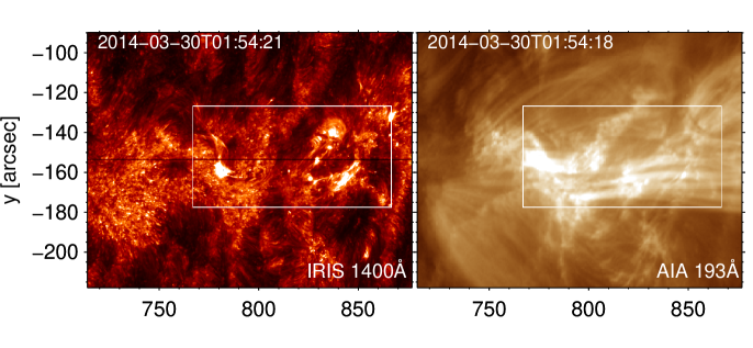
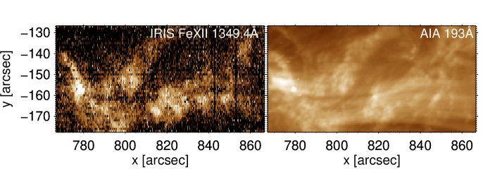
Figure 2.— IRIS and SDO-AIA observations of AR 12014. Top: IRIS slit-jaw image in the 1400Å passband (left), and AIA 193Å image (right). For a subregion, indicated by the box in the IRIS SJI and AIA images, we also show the intensity map in the Fe xii 1349Å line (from Gaussian fit to the IRIS spectra; bottom left), and the corresponding composite AIA 193Å image (built by selecting, for each horizontal slice of the IRIS f.o.v. the AIA data closest in time; bottom right).

We use IRIS calibrated level 2 data, which have been processed for dark current, flat field, and geometrical corrections (De Pontieu et al., 2014). To correct the absolute wavelength scale in the FUV, we use the neutral line of O i at 1355.6Å as our zero velocity reference since it is expected to have, on average, intrinsic velocity of less than 1 km s^-1 (when averaged along the slit; De Pontieu et al. 2014).

For both datasets we analyze simultaneous AIA (Lemen et al., 2012) level 1.5 data, processed for bad-pixel removal, despiking, flat-fielding, and image registration (coalignment among the different passbands, and adjustments of roll angle and plate scales), and Hinode-XRT (Golub et al., 2007) data, processed with the xrt_prep routine available in SolarSoft. AIA observes the full Sun at high temporal cadence ($\sim 12$s) and spatial resolution (pixel size $\sim 0.6$^′′) in several narrow EUV passbands sampling the coronal in a wide temperature range (Lemen et al., 2012; Boerner et al., 2012, 2014). Here we focus on two of the AIA passbands: the 193Å band, in which Fe xii emission is generally dominant (see e.g., Martínez-Sykora et al. 2011), and the 94Å band which is sensitive to hot plasma ($\log T[$K$]\sim 6.6-7$) because it includes a Fe xviii line (e.g., Testa et al., 2012) with strong emission in the core of active regions (e.g., Reale et al. 2011; Testa & Reale 2012). XRT observes the solar corona in soft X-ray broad bands, sensitive to a wide temperature range ($\log T[$K$]\sim 6-7.5$; e.g., Reale et al. 2009).

The EIS data are processed with SolarSoft routines that: (a) remove the CCD dark current, cosmic-ray strikes on the CCD, (b) take into account hot, warm, and dusty pixels, (c) apply radiometric calibration to convert the data to physical units, and (d) apply wavelength corrections for orbital variations and slit tilt.

We coaligned the datasets by applying a standard cross-correlation routine (tr_get_disp.pro, which is part of the IDL SolarSoftware package), to the Fe xii emission maps obtained with the different instruments. For AIA we build 193Å synthetic rasters (composite image, hereafter) by using for each stripe along a raster position (horizontal stripe for the IRIS observations we selected, and vertical for EIS) the corresponding AIA data closest in time to when the spectrograph slit was at that location. Given the uncertainties in the absolute pointing of the instruments, a few iterations are needed to find a good coalignment. In Figures 1 and 2 we show for each dataset one slit-jaw image and the AIA 193Å image closest in time, and, for a subregion scanned by the IRIS slit, we show the raster intensity map in the IRIS Fe xii 1349.4Å line, and the corresponding AIA 193Å composite image.

For the 2015-04-09 dataset the IRIS Fe xii intensity map shows the presence of elongated coronal structures and additional Fe xii fuzzy emission both above and below the bright loops. The AIA 193Å observations (Fig. 1, and movies) show that the Fe xii emission visible with IRIS corresponds to bright transient loops in the core of the active region and some bright moss. Inspection of additional AIA and Hinode-XRT data shows that these bright loops appear in the late phases of the evolution of a C6.2 flare (GOES peak at 18:51UT; see Figure 3).

In the 2014-03-29 dataset, the Fe xii emission, in both IRIS and AIA, is generally dominated by emission of bright moss, due to the high density of transition region plasma (e.g., Fletcher & De Pontieu, 1999). The AIA 94Å images and the Hinode-XRT images confirm the presence of hot dynamic loops in this active region (Figure 3).

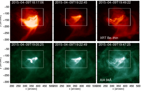
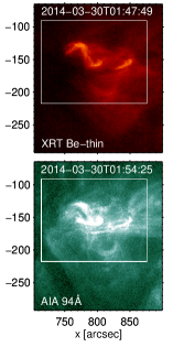
Figure 3.— Hinode-XRT (Be-thin passband) and AIA 94Å images showing the hot plasma present in the active regions we study (Figures 1 and 2). For the dataset of 2015-04-09 we show the hot plasma at three different times: the peak of the X-ray/94Å emission (first column), the peak of the hot emission in the loops that we see at a later time in Fe xii (second column), and a time closer to the IRIS and AIA images shown in Figure 1 (third column). For the moss dataset of 2014-03-30 we show the hot emission at a time close to the IRIS and AIA images of Figure 2 (fourth column). The white boxes show the f.o.v. of the IRIS SJI and AIA 193Å images shown in the top panels of Figure 1 and 2.

3. Analysis Methods and Results

The IRIS Fe xii spectral line properties are obtained by fitting the spectra with a single Gaussian (plus a constant background). The intensity maps obtained for the two datasets are shown in Figure 1 and 2, and generally show good correspondence with the brightest regions of the corresponding AIA 193Å composite images.

From the spectral fit, we derive the non-thermal line width $w_{\rm nth}=\sqrt{w^{2}_{1/e}-w^{2}_{th}-w^{2}_{instr}}$, where $w_{\rm 1/e}$ is the measured $1/e$ spectral line width (i.e., $\sqrt{2}\times$ the Gaussian $\sigma$), $w_{\rm th}$ is the thermal line width, and $w_{\rm instr}$ is the instrumental line width. The thermal line width is $\sqrt{2K_{\rm B}T/m_{\rm ion}}$, and for the temperature of peak formation of Fe xii ($\log T[K]=6.2$) it corresponds to $\sim 21.7$ km s^-1. The instrumental line width of IRIS is of the order of 4 km s^-1 (De Pontieu et al., 2014), while for our EIS dataset the instrumental line width is of order of $60-65$ km s^-1 and variable along the slit (we used the eis_slit_width SolarSoft routine to calculate the instrumental width).

 

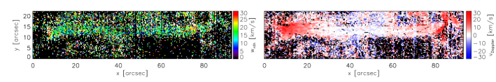
Figure 4.— Maps of Fe xii non-thermal line width (left column) and Doppler velocity (right column) from Gaussian fit to the 1349Å line in the IRIS spectra, for the two datasets of Fig. 1 (top row) and 2 (bottom row). In the Doppler velocity plots blue and red correspond to flows towards and away from the observer, respectively. In all plots black is used for pixels where the low S/N prevents a reliable determination of the velocity. In the non-thermal velocity plots white is used for pixels in which the $w_{\rm nth}$ is larger than the upper limit of the velocity scale (i.e., 30 and 25 km s^-1, for the upper and lower panel respectively).

The non-thermal line width and Doppler shift for the two selected IRIS datasets are shown in Figure 4. The non-thermal line width maps show that the typical residual observed non-thermal velocities are modest, typically of the order of $15-20$ km s^-1. The Doppler shift map of the 2015 dataset shows for the postflare loops significant redshift, more pronounced on the eastern footpoints, suggesting draining of plasma in the late phases of the flare. Moss is also visible in that observation and it shows more a mix of blue and redshifts. The histogram of Doppler velocities (top panel of Figure 5) is asymmetric, with respect to the peak, and shows a significant red shoulder due to the post-flare loop footpoints. In the observations of 2014 the moss Fe xii emission is also characterized by a mix of blue and redshifts, and the distribution (bottom panel of Figure 5) is peaked around $\sim+3$ km s^-1 (i.e., slightly redshifted), and it is significantly more symmetric than the 2015 dataset which includes the post-flare loops. We note that the line shifts we observe reveal the line of sight component of the plasma velocity: since for the moss observations of 2014-03-29 the active region is far from disk center (770^′′,-150^′′) the actual velocity of the Fe xii emitting plasma could be larger than our measured values of few km s^-1.

Figure 5.— Normalized histogram of Doppler shifts in the 1349Å IRIS Fe xii line (right panels of Figure 4), for the 2015-04-09 observations including the post-flare loops (top), and the moss observation of 2014-03-30 (bottom). The dotted line indicates zero velocity, positive velocities correspond to redshifts (i.e., velocity toward the solar photosphere), and negative velocities correspond to blueshifts (i.e., outward velocities, toward the observer). The absolute velocities are calibrated using the O i line at 1355.6Å (see sec.2).

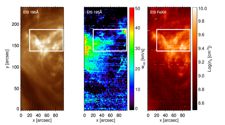
Figure 6.— Hinode-EIS observations of AR 12014 simultaneous to the IRIS and AIA observations shown in Fig. 2. We show the maps of the EIS Fe xii 195.12Å line intensities (left) and non-thermal velocities (middle), and the plasma electron densities obtained from the measured ratios of the 202Å and 203Å Fe xiii EIS lines (rigth). The box indicates the region of overlap between the EIS and the IRIS spectral observations.

We derive the EIS Fe xii 195.119Å intensity and non-thermal width by fitting the EIS spectral data with a double Gaussian to remove the blend with the weaker Fe xii line at 195.179Å. We impose that the value of the $\sigma$ of the two Gaussian components is the same, and we fix the wavelength separation $\Delta\lambda$ of the two line centroids to the separation of the theoretical wavelengths as derived from CHIANTI (see also Young et al. 2009). The maps of line intensity and non-thermal width are shown in Figure 6. In the region of overlap of the EIS and IRIS f.o.v. the Fe xii 195Å intensity morphology is very similar to the IRIS observed 1349Å emission, even though the IRIS and EIS observations are not strictly simultaneous at all locations. EIS rasters W to E, with the slit in the N-S direction. For this observation IRIS is rolled by -90 degrees, i.e., 90^∘ counterclockwise with respect to the zero degree roll (roll=0 corresponds to a N-S orientation of the slit). In this observing sequence IRIS rasters S to N (when roll=0 IRIS rasters E to W). Moss emission is typically observed to be relatively steady over timescales long compared to the $\sim 30$ min of the IRIS and EIS rasters we analyze here (Antiochos et al. 2003; Brooks et al. 2009; Tripathi et al. 2010, though see also Testa et al. 2013, 2014), therefore we expect the non-simultaneity of the spectra at each location to have limited effects on the Fe xii spectral properties derived with IRIS and EIS. We discuss more, later in this section, the extent and effects of the non-simultaneity of the observations with the two instruments.

The largest non-thermal velocities of the EIS 195Å line are observed at the footpoints of large fan loops while moss is characterized by significant smaller non-thermal motions. This is in agreement with previous studies (e.g., Doschek et al., 2008). In Figure 6 we also show a map of the plasma electron density derived from the ratio of the 202Å and 203Å Fe xiii lines (e.g., Young et al., 2009). This shows the high density of plasma in moss regions (e.g., Fletcher & De Pontieu, 1999).

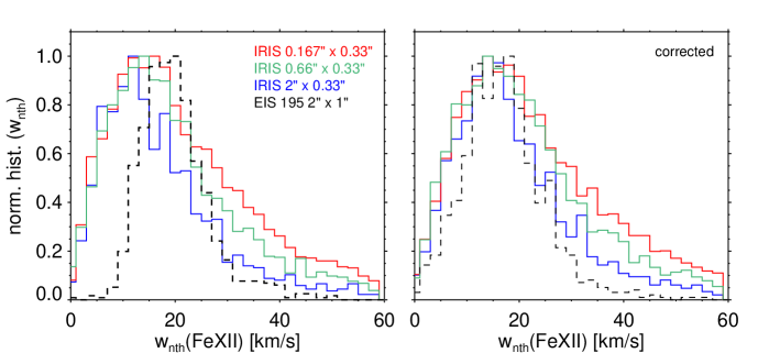
Figure 7.— Normalized histograms of non-thermal line width for the moss region where both IRIS and EIS data are available. For IRIS we show the histograms for three different rebin levels (in the slit direction, i.e., E-W): the original spatial resolution ($0.167$^′′$\times 0.33$^′′; red line), and a rebin of a factor 4 ($0.66$^′′$\times 0.33$^′′; green) and 12 ($2$^′′$\times 0.33$^′′; blue). The dashed lines corresponds to the EIS data. The right panel shows the histograms obtained by correcting for instrumental effects of both IRIS and EIS leading to systematic error in the measurements of line width (see text and Figure 8).

In Figure 7 (left panel) we compare the distributions of non-thermal velocities in the Fe xii emission observed with IRIS and with EIS. For IRIS we computed the distributions for different spatial resolution: (a) for the IRIS original spatial resolution ($0.167$^′′$\times 0.33$^′′; the width of the IRIS slit is $0.33$^′′), (b) for a rebin by a factor 4 along the slit (i.e., $0.66$^′′$\times 0.33$^′′ macropixels), and (c) for a rebin by a factor 12 ($2$^′′$\times 0.33$^′′ macropixels, i.e., only 3 times smaller than the EIS pixels). We do not integrate further because the IRIS raster for this OBSID is not “dense”, i.e., there are $\sim$1^′′ gaps in between raster positions, and even if we did sum consecutive raster positions they would not be simultaneous. The distributions of Figure 7 show that for larger rebinning factors the IRIS $w_{\rm nth}$ distributions have a smaller tail at large values. This can be expected if there is significant sub-arcsec structuring and the structures with large $w_{\rm nth}$ are generally not concentrated close to each other, and/or in the vicinity of locations with brighter narrow lines. The EIS distribution is markedly narrower than the IRIS distributions, and it also peaks at larger $w_{\rm nth}$ values ($\sim 20$ km s^-1, vs. $10-15$ km s^-1 for IRIS).

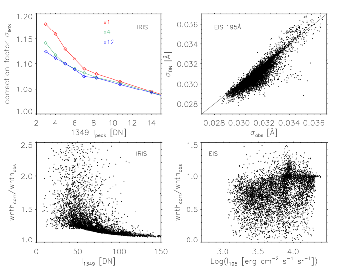
Figure 8.— Corrections of instrumental effects leading to systematic error in line width measurements. Top left: Correction factor for the Gaussian $\sigma$ in the fit to the IRIS Fe xii spectral line, as obtained from simulations (see text). Top right: Gaussian $\sigma$ from the fit of EIS Fe xii 195Å for spectra in DN units (y axis) and absolute units (x axis). Bottom: ratio of the corrected to uncorrected non-thermal widths as a function of line intensity for the IRIS 1349Å line (left), and the EIS 195Å line (right), for the region of overlap of the f.o.v. of IRIS and EIS spectral observations (see Fig. 6).

The histograms of $w_{\rm nth}$ from EIS and from IRIS for the largest rebinning factor present significant differences, whereas one would expect them to be similar. We therefore investigated possible causes for the observed large difference. For IRIS we investigated possible effects of the typically low signal-to-noise ratio on the determination of $w_{\rm nth}$: in pixels with low Fe xii signal, the wing of the Gaussian spectral line can have signal that is lower than the digitization threshold (i.e., if the signal in a spectral bin is below 1 data number [DN], the bin gets assigned a value of 0 DN), possibly leading to a systematic underestimate of the Gaussian $\sigma$. To test this hypothesis we run Monte Carlo simulations of IRIS spectra, varying the following parameters: (1) peak intensity (from 3 to 15 DN; pixels with smaller peak intensities are anyway filtered out because the fits are not reliable enough), (2) $w_{\rm nth}$ (from 5 to 20 km s^-1), (3) background value (1-16 DN/pix). For each set of parameters we run 3000 simulations applying Poisson noise to each spectral pixel, and derive the correction factor (averaged over the 3000 simulations) which multiplied by the measured $\sigma$ gives the “true” Gaussian $\sigma$ of the input model. We find that low SNR does indeed cause a slight systematic underestimation (typically by 5-15%) of $\sigma$ (and therefore of $w_{\rm nth}$), and the peak intensity is the parameter the effect mainly depends on. In Figure 8 (top left panel) we show the average correction factor for the Gaussian $\sigma$, by which the measured $\sigma$ should be multiplied to determine the actual width in the IRIS spectral fit, as a function of the peak intensity, and for different rebinning factors. In Figure 8 we also show the resulting effect on the $w_{\rm nth}$ by plotting the ratio of the corrected to “uncorrected” $w_{\rm nth}$ as a function of measured 1349Å line intensity (bottom left panel). This figure shows that the modest corrections in the Gaussian $\sigma$ can propagate to significant corrections for the non-thermal velocities.

For EIS we explored the effect of the absolute calibration (D. Brooks, priv. comm., and Brooks & Warren 2015) by comparing the Gaussian $\sigma$ obtained through the fit to the EIS spectra in physical units (erg cm^-2 s^-1 sr^-1) to the one obtained by fitting EIS spectra in DN units (obtained by applying the eis_prep SolarSoft routine with the /noabs keyword). The comparison (top right panel of Figure 8) shows that the absolute calibration leads to a systematic overestimate of the line width for most pixels. While the effect in the measured $\sigma$ is relatively small (typically $\lesssim 10$%), this propagates to significant changes of $w_{\rm nth}$. We show in the bottom right panel of Figure 8 the ratio of the corrected to “uncorrected” $w_{\rm nth}$ as a function of the 195Å line intensity.

The IRIS and EIS histograms of $w_{\rm nth}$, corrected for the above discussed instrumental effects, are shown in the right panel of Figure 7. As explained above, the correction of IRIS $w_{\rm nth}$ leads to histograms with significantly smaller numbers of pixels with low $w_{\rm nth}$, and the peaks of the histograms are around $15$ km s^-1. The correction of the EIS $w_{\rm nth}$ shifts the histogram to smaller $w_{\rm nth}$ values, and makes the distribution similar, both in terms of peak and width, to the (corrected) IRIS histogram with the largest rebinning factor, therefore largely reconciling the IRIS and EIS measurements. This analysis shows the importance of taking into account these instrumental effects, for a correct interpretation of the spectral measurements and their comparison among different instruments. The $w_{\rm nth}$ distributions in Figure 7 show the effects of spatial resolution: while all distributions at different spatial resolution are peaked around very similar values, at higher spatial resolution the distributions are broader both on the low and on the high side of the range of $w_{\rm nth}$ values. Similar results were recently found by De Pontieu et al. (2015) for Si iv transition region emission as observed by IRIS in a variety of solar features (active regions, quiet sun, coronal holes; see their Figure 2). De Pontieu et al. (2015) focus on the relative lack of sensitivity of the peak of the $w_{\rm nth}$ distributions on spatial resolution, and their possible interpretation includes: broadening processes occurring along the line-of-sight and/or on spatial scales smaller than the IRIS resolution. The broadening of the $w_{\rm nth}$ distributions at higher spatial resolution however strongly suggests that the unprecedented IRIS resolution allows us to resolve at least some structuring of the non-thermal motions at subarcsecond resolution.

We further compare the IRIS and EIS observed Fe xii spectral properties, also taking into consideration the non-simultaneity of the observations of the two instruments at all locations, due to the different roll angle and scanning direction of the two instruments. In Figure 9 (upper panel) we show the time difference between IRIS and EIS observations, in a spatial area of overlap of the two fields of view. In the other panels of Fig. 9 we use two-dimensional histograms to show the correlation of the IRIS and EIS Fe xii intensity (middle and bottom left) and corrected non-thermal line width (middle and bottom right), for pixels where the time difference is more than (middle) and less than (bottom) 300s. For IRIS we use the results obtained on data with a spatial bin of 2^′′$\times$0.33^′′, to have spatial resolution close to EIS resolution. These plots show that (a) the Fe xii intensities show stronger correlations than the non-thermal velocities, and that (b) the correlations are significantly tighter in regions where IRIS and EIS observations are less than 5 min apart, especially for the non-thermal velocity. The observed differences between IRIS and EIS results are likely due mostly to the difference in spatial pixels we compare: the IRIS macropixel we use here (2^′′$\times$0.33^′′) is three times smaller in the solar N-S direction than the corresponding EIS pixel Another possible contributing factor to observed difference between IRIS and EIS is that the EIS Fe xii 195Å line suffers significant absorption from cool chromospheric material (e.g., De Pontieu et al., 2009) which does not affect the IRIS 1349Å line.

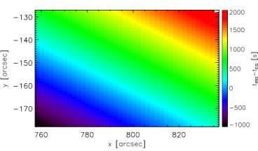
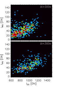
Figure 9.— Top panel: Spatial map of difference in time (in seconds) between IRIS and EIS observations in the area of overlap of the f.o.v. of the two instruments. Middle and bottom panels: 2-dimensional histograms showing the correlation between intensity in Fe xii lines (left panels) and non-thermal line widths (right panels) as measured by IRIS (1349Å line; spatially integrated by a factor 12, i.e., with a spatial bin of 2^′′$\times$0.33^′′), and EIS (195Å line, at the original spatial resolution, i.e., with a pixel of 2^′′$\times$1^′′). The middle and bottom panels show the 2D histograms (i.e., the two dimensional joint probability density function) for the subset of spatial pixels where the difference in time between IRIS and EIS observations is $\gtrsim 300$ s and $\lesssim 300$ s respectively. We use the rainbow color bar (as in top panel), so red corresponds to the highest pixel density (followed by orange, yellow, green, cyan, blue, black).

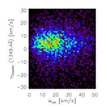
Figure 10.— Left: Correlation between non-thermal line widths (corrected for the systematic effects; see Fig. 8 and text) and line intensities for the Fe xii lines in IRIS (1349Å; top) and EIS (195Å; bottom), for the region of overlap of the f.o.v. of the two spectrographs. Right: 2D histogram of the IRIS Fe xii measured non-thermal velocities (x axis) and Doppler shifts (y axis). This plot shows an apparent lack of correlation between the two derived quantities. For both plots, we selected only the pixels where the Fe xii intensity was larger than a threshold value in order to identify the moss.

We investigate the presence of correlations between non-thermal width, line intensity, and Doppler shifts, which have been found in several previous spectral studies of active region coronal emission. In Figure 10 we plot $w_{\rm nth}$ as a function of the line intensity for both the IRIS 1349Å line and the EIS 195Å line. These plots show the presence of some positive, though weak, correlation between $w_{\rm nth}$ and line intensity, and that the correlation is more pronounced at the significantly higher spatial resolution of IRIS. Significant fine structuring of the Fe xii emission on spatial scales unresolved by EIS could explain this result: if $w_{\rm nth}$ is correlated with line intensity, locally, – which is plausible as larger non-thermal velocities could be associated with larger heating, as in the predictions of several models (e.g., Cargill, 1996; Asgari-Targhi et al., 2014) – and significant structuring is present on small spatial scale, a higher spatial resolution would allow to observe more clearly the correlation between $w_{\rm nth}$ and intensities, which would get washed out when integrating on spatial scales significantly larger than the scales of typical structuring. The observed behavior of $w_{\rm nth}$ vs. line intensity provides clues to whether noise might be a dominating factor in the determination of $w_{\rm nth}$ from the IRIS spectra: if the large $w_{\rm nth}$ values, largely absent in EIS spectra, were attributable to noise, we would expect some anticorrelation of $w_{\rm nth}$ with intensity, with most of the high $w_{\rm nth}$ values associated with low line intensities (therefore noisier spectra); this is not what we observe, therefore the high $w_{\rm nth}$ values are likely real. The $w_{\rm nth}$ does not appear to have significant correlation with the Doppler velocity (Figure 10).

Figure 11.— Comparison of distributions of Doppler shifts (top panel) and non-thermal width (bottom panel) observed with IRIS in moss of AR 12014 at different viewing angles, and at the highest spatial resolution ($\sim 0.167$^′′$\times 0.33$^′′). We compare the dataset of 2014-03-30, which we analyzed in detail in the rest of the paper, with an IRIS observation of AR 12014 on 2014-03-26 (00:57UT-01:30UT) when the active region was close to disk center (center of IRIS f.o.v. at x,y=52.9,-92.8).

The distributions of Doppler shifts (see Fig. 5) and non-thermal line width (Fig. 7) we found for the Fe xii emission observed with IRIS can have in principle significant dependencies on the viewing angles. To explore these effects we consider an additional IRIS observation of AR 12014 on 2014-03-26 (starting at 00:57UT, i.e., about 4 days prior to the IRIS observation of AR 12014 we studied in detail in the rest of the paper), when the active region was close to disk center (center of IRIS f.o.v. at x,y=52.9,-92.8), and using the same IRIS OBSID (3810263243). Carrying out the same processing and analysis of the IRIS spectra we obtain the distributions of Doppler shifts and non-thermal velocities, and compare them, in Figure 11, to the results of the observations of 2014-03-30 when the AR is closer to the limb. We note that any difference between the two observations at different viewing angle can in principle be caused by both the viewing angle and by intrinsic differences of the physical conditions, e.g., due to active region evolution and different activity level at the two times. The Doppler shift distribution for the disk center case is broader than for the case at higher inclination. This could be expected if a significant portion of the line shifts were due to velocity in a direction close to the local vertical direction: viewed at a larger angle, the line-of-sight component of those velocities would become smaller both on the blue and red side. However, for the observation at high angle (i.e., when the AR is closer to the limb) the distribution is not only narrower but also appears redshifted. This could be interpreted as an effect of a slightly higher activity level at that time (see discussions in § 4 and 5). The non-thermal velocity distributions are quite similar to each other, with the disk center observations showing a larger portion of pixels at high velocity values ($w_{\rm nth}$$\gtrsim 20$km s^-1). This result suggests that field aligned flows significantly contribute to the observed $w_{\rm nth}$, as also suggested by De Pontieu et al. (2015).

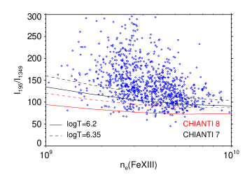
Figure 12.— Observed intensity ratio (in erg cm^-2 s^-1 sr^-1) of 195Å EIS line and 1349Å IRIS Fe xii line (blue diamond symbols). We show the theoretical ratio from the CHIANTI atomic database (version 7, red, and version 8, black) for two different temperatures ($\log T[K]=6.2$, solid lines, and $\log T[K]=6.35$, dashed lines).

Finally, we computed the ratios of the measured Fe xii line intensities of the IRIS 1349Å line and the EIS 195Å line, and compared them with the predictions of the CHIANTI database (Figure 12). In order to calculate this ratio we used the Fe xii 1349Å line intensity measured from the IRIS spectra rebinned to a 2^′′$\times$0.33^′′ spatial scale, and we converted them to physical units (erg cm^-2 s^-1 sr^-1). The uncertainties in the effective areas of IRIS and EIS are expected to be of the order of 20-25% (De Pontieu et al. 2014; Lang et al. 2006; Del Zanna 2013; Warren et al. 2014). We calculated the CHIANTI predicted line ratios using the last two CHIANTI versions (in the just released v.8 of CHIANTI, some of the Fe xii data in the EUV wavelength range have significantly changed), and for two different temperatures. The comparison between the observed and the theoretical values shows that the atomic data systematically underestimate the 195Å/1349Å ratio (i.e., they predict a stronger than observed 1349Å line, compared with the 195Å line), and that the discrepancy is larger for CHIANTI 8. We note that in reality the extent of the underestimate is likely even larger, because the 195Å emission in moss is expected to suffer significant (typically a factor $\sim 2$) absorption from cool chromospheric material, which affects wavelengths below 912Å, and it is due to resonance continua of neutral hydrogen and helium (De Pontieu et al., 2009).

4. 3D radiative MHD simulations

In order to gain insight into the observed Fe xii spectral properties of active region moss we consider ‘realistic’ 3D radiative MHD simulations of the solar atmosphere using the Bifrost code (Gudiksen et al., 2011). The Bifrost code solves the full resistive MHD equations, including non-LTE and non-grey radiative transfer with scattering, and with thermal conduction along the magnetic field lines. The model spans from the upper layer of the convection zone up to the low corona, and self-consistently produces a chromospheric and hot corona, through the Joule dissipation of electrical currents that arise as a result of foot point braiding in the photosphere and convection zone (Hansteen et al., 2015).

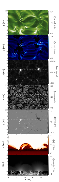
Figure 13.— Spatial distribution of several physical variables in the Bifrost simulation we analyze here. From top to bottom: (a) top view Fe xvi (335Å) intensity showing the structure of the $\sim 2-3$ MK corona; (b) top view of Fe xii (195Å) intensity showing that the highest intensity regions consist of moss-like areas at the footpoints of hot loops; (c) top view line intensity of bin4 intensity (see text) with opacity typical of a strong chromospheric line; (d) top view intensity of the bin1 (low opacity, see text) emission typical of the solar continuum emission in the visible; (e) top view intensity of vertical component of magnetic field; (f) side view of plasma temperature; (g) side view of magnetic field intensity. The white dashed line in the top five panels shows the location of the vertical cut displayed in the bottom two panels.

Here we consider a Bifrost simulation yielding a high temperature corona ($\gtrsim 5$ MK) and therefore having strong Fe xii emission closer to the loop footpoints (i.e., “moss”; see Figure 13). The simulation covers a region of dimensions $24\times 24\times 17$ Mm³, with $768\times 768\times 768$ grid points ($\Delta x=\Delta y\sim 31$ km, $\Delta z\approx 13$ km up to a height of 5 Mm above the photosphere and increasing to $\approx 80$ km at the top of the computational box).

The magnetic field configuration of this model is very similar to that found in the publicly available simulation published as part of the IRIS project and described in Carlsson et al. (2016). In both models the photospheric field is dominated by two concentrated opposite polarity regions of approximately equal strength that are some 10 Mm apart. This configuration gives a set of loops in the chromosphere and corona connecting the opposite polarity regions. In addition (and as opposed to the publicly available model) a weaker, 100 G, horizontal field is continuously injected at the bottom boundary, 2.5 Mm below the photosphere. This injection eventually leads to a weaker ‘salt and pepper’ field that fills the entire photosphere at the time of the model snapshots presented here. The additional magnetic field alters the atmospheric conditions sufficiently to raise the coronal temperature well above what is found in the publicly available model. It is the upwardly directed Poynting flux, generated by the interaction of the photospheric motions with the magnetic field, that ultimately heats the outer layers of the model to high temperatures.

Figure 13 shows the spatial distribution of several physical variables for a snapshot of the Bifrost simulation near the time of largest coronal temperatures and analyzed here; we show side views of the total magnetic field and temperature and top views of the vertical component, $B_{z}$, of the photospheric field, the continuum, chromospheric and transition region and coronal intensities. The optically thick radiative losses are computed by binning solar opacities into four bins, sorted according to magnitude, as described by Nordlund (1982); Skartlien (2000); Hayek et al. (2010). In Figure  13 we show the emission in bin 1 (similar to white light emission with an effective temperature of approximately 5800K), which represents the lowest opacities, and bin 4 which represents the highest opacities of those considered. Bin 1 is similar to continuum emission at visible wavelengths in the solar spectrum, while bin 4 is typical of a strong chromspheric line such as Ca ii H or K. The strong magnetic field concentrated in the photosphere rapidly spreads in the chromosphere and forms loop-like structures connecting the opposite polarity regions that penetrate into the corona. High temperature coronal material penetrates to within a 1 Mm of the photosphere in the vicinity of the footpoints of these loops. The synthetic images in the Fe xvi and Fe xii emission show that the simulated atmosphere has hot loop-like coronal structures, and the highest Fe xii emission is concentrated at the footpoint of hot, dense loops. Therefore we can use the synthetic Fe xii emission as a comparison with our moss observations.

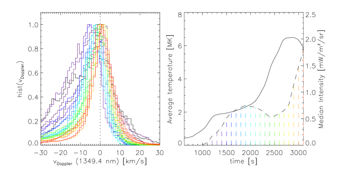
Figure 14.— Left: Histograms of Doppler velocity distributions of Fe xii emission in the Bifrost 3D MHD simulation at different times in the evolution of the atmosphere (see right panel for the correspondence between time and color). Right: Evolution of temperature (solid line) and Fe xii median intensity (dashed line) in the Bifrost simulation.

From the Bifrost simulation we calculate the Doppler shift and the non-thermal width of the 1349Å IRIS line, to compare it with our IRIS observations. In the IRIS observation, the sensitivity of the instrument effectively selects only the brightest Fe xii emission regions, i.e., the moss. For a more meaningful comparison with the IRIS observations we calculate the distributions of the Fe xii spectral properties on a subset of the simulation volume, where the Fe xii is highest (i.e., at the footpoints of hot loops), using $3\times$ the median intensity as a threshold value. We also integrate the Fe xii emission on the same spatial resolution as with IRIS, and integrate over 30 s; note that we have one snap shot every 10 s, therefore we may underestimate the range of dynamics that is present in both the model and the real solar atmosphere on much smaller temporal scales.

In Figure 14 we show the histograms of the 1349Å Fe xii Doppler shift for a series of snapshots (one every 100 s) in the interval 1000-3000 s from the start of the simulation. As the atmosphere is heated to high coronal temperatures (the average temperature in the simulation box is plotted in the right panel of Figure 14), the peak of the Doppler shift distribution goes from blueshifts (upflow) of 5-10 km s^-1, via smaller blueshifts, and finally to low amplitude redshifts (downflow) of some few km s^-1. This can be explained by the fact that Fe xii is shifting from being emitted mainly from coronal plasma, when the corona is relatively cool ($\lesssim 2$ MK), to being emitted from transition region plasma, confined by a large temperature gradient, when the corona gets hotter. As the coronal temperature increases, the plasma most strongly emitting Fe xii lines (i.e., plasma typically at 1-1.5 MK) becomes more and more confined to the lower layers of coronal structures (i.e., at the loop footpoints) and therefore the observed Fe xii lines behave more like typical transition region lines, generally dominated by redshifts. Both Peter et al. (2006) using the Stagger code, and Hansteen et al. (2010) using Bifrost simulations found that the observed net transition region redshifts were reproduced in 3D ’realistic’ numerical models. As described in Hansteen et al. (2010), in the Bifrost simulations, redshifts of the transition region emission are a consequence of the episodic heating and concentration of the heating per particle in the lower atmosphere: the plasma is heated at lower heights to high temperature, and the increased pressure causes upflows in the hotter lines and downflows in the cooler (transition region) lines. The evolution of median intensity of Fe xii emission as a function of time in the simulation is also shown in the right panel of Figure 14. The Fe xii intensity initially increases as the coronal temperature increases from initial values of $\sim 0.5$ MK to $\sim 2$ MK. As the coronal temperature continues to increase, the Fe xii emission initially decreases as less and less of the coronal volume emits Fe xii since it becomes too hot. Later ($t>2500$ s) the emission increases again, and steeply, as the Fe xii emission is “pushed” to steadily denser transition region layers.

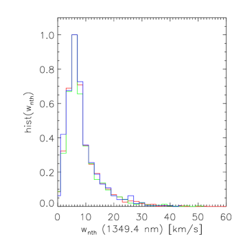
Figure 15.— For the Bifrost snapshot at time t=3050 s, when the coronal temperature is close to its peak (see Figure 14), we show the histograms of Fe xii non-thermal line width distributions for the same spatial binning used for the analysis of the IRIS data, with the same color coding of Figure 7: red for the IRIS original spatial resolution ($0.167$^′′$\times 0.33$^′′), green for a rebin of a factor 4 ($0.66$^′′$\times 0.33$^′′), and blue for a rebin of a factor 12 ($2$^′′$\times 0.33$^′′).

In Figure 15 we plot the histogram of the non-thermal line widths of the Fe xii 1349Å emission from the Bifrost simulation (for a snapshot where the average coronal temperature is $\sim 6$ MK). The spectral line profiles are synthesized from the Bifrost snapshot by using the IRIS spectral, spatial and temporal resolution, and selecting only the strongest emission regions (as described above). After IRIS-like spectra are obtained, they have been analyzed at three different levels of spatial binning, just like for the actual data (see Figure 7). The non-thermal line widths, $w_{\rm nth}$, are then calculated as for the actual spectra by subtracting instrumental and thermal broadening (see beginning of § 3). The $w_{\rm nth}$ distributions from the Bifrost simulation peak at lower values ($\sim 7$ km s^-1) than for the observations ($\sim 15$ km s^-1, see Figure 7), and they are also characterized by narrower distributions. The limited non-thermal broadening from Bifrost simulations compared with observations has been observed and discussed in previous papers Hansteen et al. (2010); Olluri et al. (2015). The effect of decreased spatial resolution (i.e., larger spatial bin) in the simulated spectra is similar but not identical to that seen for the actual data: at lower spatial resolution the peak of the $w_{\rm nth}$ distribution does not change, but in contrast with the data, we do not see any narrowing of the distribution with higher spatial resolution, except in certain subsets.

5. Discussion and conclusions

We have presented a first analysis of IRIS Fe xii spectral observations at the highest spatial resolution to date, which show the presence of fine coronal structure on subarcsecond scale. In particular we have shown that Fe xii emission can be observed with IRIS in bright (dense) coronal structures such as post-flare loops, and active region moss, by adopting long exposure times, and lossless compression.

The presence of neutral lines in the IRIS spectra allow an accurate absolute wavelength calibration, and therefore a more accurate determination of line Doppler shifts, compared to some other spectral observations, e.g., with EIS. For the post-flare loops we find that the Fe xii emission is largely unshifted at the loop tops and predominantly redshifted at both loop footpoints, as expected for draining of plasma in the later phases of the flare when the heating has ceased. For the moss observations, we find that the distribution of Doppler shifts is peaked at a redshift of a few km s^-1, but with significant wings on both the red and the blue side. In our interpretation, guided by the Bifrost 3D models, Fe xii appears redshifted for hotter coronal temperatures ($\gtrsim 4$MK), while blueshifted when the corona is at cooler temperatures. The distribution of Doppler shift we observe shows a wide range of blue and red shifts, and it suggests that there may be a continuous mix of heating and cooling in the moss we observed. For cooler transition region lines ($\log T$[K]$\sim 4.7-5.7$) the dominance of redshift is well established (e.g., Doschek et al., 1976; Dere et al., 1984; Achour et al., 1995; Chae et al., 1998b; Peter & Judge, 1999). The physical processes causing the observed redshifts are still debated, and several models have been proposed (e.g., Hansteen, 1993; Patsourakos & Klimchuk, 2006; Peter et al., 2006; Hansteen et al., 2010). Hansteen et al. (2010) use 3D radiative MHD models of the solar atmosphere to investigate the transition region redshifts, and find that in their model the heating is dominated by rapid intermittent events at low heights which heat the plasma locally to coronal temperature and produces downflows at transition region temperature due to the local overpressure. The model analyzed by Hansteen et al. (2010) reached modest coronal temperatures ($\lesssim 2.5$ MK), therefore with significant Fe xii emission in loop structures rather than at the loop footpoints as in the case for moss. Here we used a different Bifrost 3D MHD simulation which reaches higher coronal temperature and represent a better model for moss observations. We find that the moss Fe xii (mostly) redshifted emission we observe with IRIS is reproduced in the model when the corona gets hot enough and most of the Fe xii is confined in the loops transition region. The Fe xii then behaves like a transition region line, and is redshifted, in the model, as a consequence of the local heating at low heights which causes upflows in the hotter lines and downflows in the cooler (transition region) lines.

We also analyzed the Fe xii line broadening, in both IRIS and EIS moss observations, and find that the non-thermal broadening is typically small (the distributions peak around 15 km s^-1) and the $w_{\rm nth}$ distributions are generally similar at different spatial resolution scales, as found also by De Pontieu et al. (2015) for the cooler IRIS Si iv emission. However, we find that at the higher spatial resolution accessible with IRIS the $w_{\rm nth}$ histograms are broader. The fact that at higher resolution, higher values of $w_{\rm nth}$ are observed, is somewhat counterintuitive, if interpreting the $w_{\rm nth}$ as due to unresolved motions along the line-of-sight. The higher $w_{\rm nth}$ observed at higher spatial resolution must come from spatially separate events, occurring on a spatial scale typically smaller than IRIS spatial resolution, and with intrinsic large mixing of velocities along the line-of-sight. These features are possibly associated to heating events.

We discussed in detail systematic effects affecting the line broadening measurements in both IRIS and EIS: low signal-to-noise ratio leads to systematic underestimates of $w_{\rm nth}$ from IRIS spectra, while the absolute calibration of EIS causes systematic overestimates of $w_{\rm nth}$ (see Brooks & Warren 2015). These effects need to be taken into account for a correct measurement and interpretation of the spectral lines broadening. We analyzed the non-thermal broadening in the Bifrost 3D model and find that the $w_{\rm nth}$ are systematically smaller than in the observations (the distributions peak around 10 km s^-1) but otherwise they are affected by spatial resolution in a similar way to the observations. We note however that the comparison of the modeled and observed velocities might be significantly affected by the viewing angle. The low average $w_{\rm nth}$ that we find from the Fe xii spectral analysis are in agreement with several previous findings (e.g., Dere & Mason 1993; Brooks et al. 2009, though at coarser spatial resolution), but at the IRIS subarcsecond resolution we also find a significant tail at larger $w_{\rm nth}$ values, which can further constrain the models. In particular, the high $w_{\rm nth}$ values might be missing in current models because of insufficient spatial resolution, as test simulations at higher resolution show a significant increase in turbulence, vorticity and small-scale flows in the solar atmosphere that could lead to significant non-thermal broadening in the atmosphere. In addition, preliminary results suggest that the mix of strong fields and neighboring mixed polarity weaker fields plays an important role in creating atmospheric dynamics. Therefore, simulations with different photospheric magnetic field distributions could well lead to an increase of non-thermal line broadening. Brooks & Warren (2015) recently investigated the non-thermal broadening of hot lines (up to $\sim 5$ MK; see also Imada et al. 2009) in the core of active regions and find that they are very modest ($\lesssim 15$ km s^-1; though see also Saba & Strong 1991). The hot line measurements by Brooks & Warren (2015) are made in the coronal portion of hot loops at the footpoints of which is the moss. Our $w_{\rm nth}$ results together with Brooks & Warren (2015), assuming that both are typical of active regions, suggest that the $w_{\rm nth}$ does not increase with temperature, in disagreement with some models (e.g., Patsourakos & Klimchuk, 2006). As discussed in § 3 and here above, the measured velocities (both Doppler shifts and non-thermal velocities) will be affected by the viewing angle. We investigated the possible viewing angle effects by comparing IRIS Fe xii observations of the same active region moss for significantly different angles. The observations we considered were taken 4 days apart therefore some differences are likely due to active region evolution. However, the fact that the $w_{\rm nth}$ distribution is broader for the near disk center observation, compared to the near limb observation, seem to indicate that the field aligned velocities provide a significant contribution to the $w_{\rm nth}$. In a scenario in which the $w_{\rm nth}$ were largely due to velocities perpendicular to the field lines (e.g., for Alfv$\acute{\rm e}$n wave turbulence models; e.g., van Ballegooijen et al. 2011, 2014) we would expect smaller $w_{\rm nth}$ for observations near disk center, for which our line of sight is expected to be more parallel to field lines on average.

Previous spectral studies of active region coronal emission have explored correlations between non-thermal width, line intensity, and Doppler shifts. In our analysis we find for Fe xii no correlation between Doppler shifts and non-thermal widths, and a weak correlation between $w_{\rm nth}$ and line intensities. Early studies with HRTS focused on cooler transition region lines (e.g., C iv, Si iv), and found some correlation between $w_{\rm nth}$ and line intensities (e.g., Dere et al., 1984; Dere & Mason, 1993). SUMER analyses expanded on these early findings, however, mostly focusing on quiet sun observations as only few on-disk active region SUMER observations are available to compare with our observations. Quiet sun SUMER studies have generally found some level of correlation between $w_{\rm nth}$ and line intensity, e.g., in O iv, O v, N v, Si iv (e.g., Warren et al., 1997; Landi et al., 2000; Akiyama et al., 2005). A comprehensive QS study by Chae et al. (1998a) explored the $w_{\rm nth}$-intensity correlation for a broad range of temperatures and found that the two parameters are correlated for lines emitted at temperatures in the $2\times 10^{4}-10^{5}$ K range, but the correlation becomes significantly weaker for hotter lines. SUMER observations including active regions show some cases where the $w_{\rm nth}$-intensity correlation is not very clear (possibly because of the mixing of different types of solar coronal features; e.g., Spadaro et al. 2000), and some cases where $w_{\rm nth}$ appears correlated with intensity for cooler lines (up to C iv) but not for the hotter Ne viii line (Feldman et al. 2011, echoing the QS results of Chae et al. 1998a). More recently, Hinode-EIS studies have analyzed the possible correlations of $w_{\rm nth}$ and line intensity for a wide range of spectral lines (and plasma temperatures), and coronal features. The correlation of $w_{\rm nth}$ and Doppler velocity is mostly found in outflow regions at the edges of active regions (e.g., Doschek et al., 2008), while the two are not correlated in moss (Doschek, 2012). Li & Ding (2009) and Scott & Martens (2011) investigate the correlations between $w_{\rm nth}$ and line intensities and find contrasting results: positive correlation (Li & Ding, 2009) or negative correlation (Scott & Martens, 2011). We argue that different studies include varied combinations of solar features, significantly affecting the presence of correlations. Also, these cited previous studies do not specifically address moss emission and therefore make for a poor comparison with our results.

In conclusion, in this work we analyzed spectral observations of Fe xii emission, for the first time at subarcsecond resolution accessible with IRIS, in particular focusing on the Doppler shifts and non-thermal widths of the emission of active region moss. We find that Fe xii moss emission is mildy redshifted on average, and shows broad distributions of Doppler shifts. These characteristics are reproduced by a 3D MHD Bifrost simulation with a hot corona ($\gtrsim 4$ MK), in which the Fe xii emission is largely confined to the transition region and shows redshifts caused by episodic heating in the low solar atmosphere. For the non-thermal line width distribution we find that the peak does not appear to depend on spatial resolution, but with increasing resolution the distributions become broader with both more low and high values of non-thermal line broadening. Analogous results have been found for Si iv emission observed with IRIS (De Pontieu et al., 2015). If the tail of high $w_{\rm nth}$ values is due to heating events, it suggests that these events typically happen on small (subarcsecond) spatial scales, and their temporal frequency is such that not many of them happen simultaneously on arcsecond scale areas. Finally, our observations of the same active region from different viewing angles show a slight increase in non-thermal broadening at disk center suggesting that field-aligned flows contribute significantly to the broadening. Our results provide constraints for heating models based on Alfvenic turbulence which predict increased broadening for viewing angles perpendicular to the magnetic field.

References

- Achour et al. (1995) Achour, H., Brekke, P., Kjeldseth-Moe, O., & Maltby, P. 1995, ApJ, 453, 945
- Akiyama et al. (2005) Akiyama, S., Doschek, G. A., & Mariska, J. T. 2005, ApJ, 623, 540
- Antiochos et al. (2003) Antiochos, S. K., Karpen, J. T., DeLuca, E. E., Golub, L., & Hamilton, P. 2003, ApJ, 590, 547
- Antolin et al. (2015) Antolin, P., Vissers, G., Pereira, T. M. D., Rouppe van der Voort, L., & Scullion, E. 2015, ApJ, 806, 81
- Asgari-Targhi et al. (2014) Asgari-Targhi, M., van Ballegooijen, A. A., & Imada, S. 2014, ApJ, 786, 28
- Athay et al. (1983) Athay, R. G., Gurman, J. B., Henze, W., & Shine, R. A. 1983, ApJ, 265, 519
- Bartoe (1982) Bartoe, J.-D. F. 1982, Advances in Space Research, 2, 185
- Berger et al. (1999) Berger, T. E., De Pontieu, B., Schrijver, C. J., & Title, A. M. 1999, ApJ, 519, L97
- Boerner et al. (2012) Boerner, P., Edwards, C., Lemen, J., Rausch, A., Schrijver, C., Shine, R., Shing, L., Stern, R., Tarbell, T., Title, A., Wolfson, C. J., Soufli, R., Spiller, E., Gullikson, E., McKenzie, D., Windt, D., Golub, L., Podgorski, W., Testa, P., & Weber, M. 2012, Sol. Phys., 275, 41
- Boerner et al. (2014) Boerner, P. F., Testa, P., Warren, H., Weber, M. A., & Schrijver, C. J. 2014, Sol. Phys., 289, 2377
- Brooks & Warren (2015) Brooks, D. H., & Warren, H. P. 2015, ArXiv e-prints
- Brooks et al. (2009) Brooks, D. H., Warren, H. P., Williams, D. R., & Watanabe, T. 2009, ApJ, 705, 1522
- Brueckner (1981) Brueckner, G. E. 1981, in Solar Active Regions: A monograph from Skylab Solar Workshop III, ed. F. Q. Orrall, 113–127
- Cargill (1996) Cargill, P. J. 1996, Sol. Phys., 167, 267
- Carlsson et al. (2016) Carlsson, M., Hansteen, V. H., Gudiksen, B. V., Leenaarts, J., & De Pontieu, B. 2016, A&A, 585, A4
- Chae et al. (1998a) Chae, J., Schühle, U., & Lemaire, P. 1998a, ApJ, 505, 957
- Chae et al. (1998b) Chae, J., Yun, H. S., & Poland, A. I. 1998b, ApJS, 114, 151
- Cheng et al. (1979) Cheng, C.-C., Doschek, G. A., & Feldman, U. 1979, ApJ, 227, 1037
- Cook et al. (1994) Cook, J. W., Keenan, F. P., Harra, L. K., & Tayal, S. S. 1994, ApJ, 429, 924
- Culhane et al. (2007) Culhane, J. L., Harra, L. K., James, A. M., Al-Janabi, K., Bradley, L. J., Chaudry, R. A., Rees, K., Tandy, J. A., Thomas, P., Whillock, M. C. R., Winter, B., Doschek, G. A., Korendyke, C. M., Brown, C. M., Myers, S., Mariska, J., Seely, J., Lang, J., Kent, B. J., Shaughnessy, B. M., Young, P. R., Simnett, G. M., Castelli, C. M., Mahmoud, S., Mapson-Menard, H., Probyn, B. J., Thomas, R. J., Davila, J., Dere, K., Windt, D., Shea, J., Hagood, R., Moye, R., Hara, H., Watanabe, T., Matsuzaki, K., Kosugi, T., Hansteen, V., & Wikstol, Ø. 2007, Sol. Phys., 243, 19
- Dadashi et al. (2012) Dadashi, N., Teriaca, L., Tripathi, D., Solanki, S. K., & Wiegelmann, T. 2012, A&A, 548, A115
- De Pontieu et al. (1999) De Pontieu, B., Berger, T. E., Schrijver, C. J., & Title, A. M. 1999, Sol. Phys., 190, 419
- De Pontieu et al. (2015) De Pontieu, B., McIntosh, S., Martinez-Sykora, J., Peter, H., & Pereira, T. M. D. 2015, ApJ, 799, L12
- De Pontieu et al. (2009) De Pontieu, B., McIntosh, S. W., Hansteen, V. H., & Schrijver, C. J. 2009, ApJ, 701, L1
- De Pontieu et al. (2014) De Pontieu, B., Title, A. M., Lemen, J. R., Kushner, G. D., Akin, D. J., Allard, B., Berger, T., Boerner, P., Cheung, M., Chou, C., Drake, J. F., Duncan, D. W., Freeland, S., Heyman, G. F., Hoffman, C., Hurlburt, N. E., Lindgren, R. W., Mathur, D., Rehse, R., Sabolish, D., Seguin, R., Schrijver, C. J., Tarbell, T. D., Wülser, J.-P., Wolfson, C. J., Yanari, C., Mudge, J., Nguyen-Phuc, N., Timmons, R., van Bezooijen, R., Weingrod, I., Brookner, R., Butcher, G., Dougherty, B., Eder, J., Knagenhjelm, V., Larsen, S., Mansir, D., Phan, L., Boyle, P., Cheimets, P. N., DeLuca, E. E., Golub, L., Gates, R., Hertz, E., McKillop, S., Park, S., Perry, T., Podgorski, W. A., Reeves, K., Saar, S., Testa, P., Tian, H., Weber, M., Dunn, C., Eccles, S., Jaeggli, S. A., Kankelborg, C. C., Mashburn, K., Pust, N., Springer, L., Carvalho, R., Kleint, L., Marmie, J., Mazmanian, E., Pereira, T. M. D., Sawyer, S., Strong, J., Worden, S. P., Carlsson, M., Hansteen, V. H., Leenaarts, J., Wiesmann, M., Aloise, J., Chu, K.-C., Bush, R. I., Scherrer, P. H., Brekke, P., Martinez-Sykora, J., Lites, B. W., McIntosh, S. W., Uitenbroek, H., Okamoto, T. J., Gummin, M. A., Auker, G., Jerram, P., Pool, P., & Waltham, N. 2014, Sol. Phys., 289, 2733
- Del Zanna (2013) Del Zanna, G. 2013, A&A, 555, A47
- Del Zanna et al. (2015) Del Zanna, G., Dere, K. P., Young, P. R., Landi, E., & Mason, H. E. 2015, A&A, 582, A56
- Dere (1982) Dere, K. P. 1982, Sol. Phys., 77, 77
- Dere et al. (1984) Dere, K. P., Bartoe, J.-D. F., & Brueckner, G. E. 1984, ApJ, 281, 870
- Dere et al. (1997) Dere, K. P., Landi, E., Mason, H. E., Monsignori Fossi, B. C., & Young, P. R. 1997, A&AS, 125, 149
- Dere & Mason (1993) Dere, K. P., & Mason, H. E. 1993, Sol. Phys., 144, 217
- Doschek (2012) Doschek, G. A. 2012, ApJ, 754, 153
- Doschek et al. (1976) Doschek, G. A., Bohlin, J. D., & Feldman, U. 1976, ApJ, 205, L177
- Doschek & Feldman (1977) Doschek, G. A., & Feldman, U. 1977, ApJ, 212, L143
- Doschek et al. (1981) Doschek, G. A., Mariska, J. T., & Feldman, U. 1981, MNRAS, 195, 107
- Doschek et al. (2008) Doschek, G. A., Warren, H. P., Mariska, J. T., Muglach, K., Culhane, J. L., Hara, H., & Watanabe, T. 2008, ApJ, 686, 1362
- Feldman et al. (2011) Feldman, U., Dammasch, I. E., & Doschek, G. A. 2011, ApJ, 743, 165
- Feldman et al. (1983) Feldman, U., Doschek, G. A., & Cohen, L. 1983, ApJ, 273, 822
- Fletcher & De Pontieu (1999) Fletcher, L., & De Pontieu, B. 1999, ApJ, 520, L135
- Galsgaard & Nordlund (1996) Galsgaard, K., & Nordlund, Å. 1996, J. Geophys. Res., 101, 13445
- Golub et al. (2007) Golub, L., Deluca, E., Austin, G., Bookbinder, J., Caldwell, D., Cheimets, P., Cirtain, J., Cosmo, M., Reid, P., Sette, A., Weber, M., Sakao, T., Kano, R., Shibasaki, K., Hara, H., Tsuneta, S., Kumagai, K., Tamura, T., Shimojo, M., McCracken, J., Carpenter, J., Haight, H., Siler, R., Wright, E., Tucker, J., Rutledge, H., Barbera, M., Peres, G., & Varisco, S. 2007, Sol. Phys., 243, 63
- Gudiksen et al. (2011) Gudiksen, B. V., Carlsson, M., Hansteen, V. H., Hayek, W., Leenaarts, J., & Martínez-Sykora, J. 2011, A&A, 531, A154
- Gudiksen & Nordlund (2005) Gudiksen, B. V., & Nordlund, Å. 2005, ApJ, 618, 1020
- Hansteen (1993) Hansteen, V. 1993, ApJ, 402, 741
- Hansteen et al. (2015) Hansteen, V., Guerreiro, N., De Pontieu, B., & Carlsson, M. 2015, ApJ, 811, 106
- Hansteen et al. (2010) Hansteen, V. H., Hara, H., De Pontieu, B., & Carlsson, M. 2010, ApJ, 718, 1070
- Hayek et al. (2010) Hayek, W., Asplund, M., Carlsson, M., Trampedach, R., Collet, R., Gudiksen, B. V., Hansteen, V. H., & Leenaarts, J. 2010, A&A, 517, A49
- Imada et al. (2009) Imada, S., Hara, H., & Watanabe, T. 2009, ApJ, 705, L208
- Klimchuk (2006) Klimchuk, J. A. 2006, Sol. Phys., 234, 41
- Kosugi et al. (2007) Kosugi, T., Matsuzaki, K., Sakao, T., Shimizu, T., Sone, Y., Tachikawa, S., Hashimoto, T., Minesugi, K., Ohnishi, A., Yamada, T., Tsuneta, S., Hara, H., Ichimoto, K., Suematsu, Y., Shimojo, M., Watanabe, T., Shimada, S., Davis, J. M., Hill, L. D., Owens, J. K., Title, A. M., Culhane, J. L., Harra, L. K., Doschek, G. A., & Golub, L. 2007, Sol. Phys., 243, 3
- Landi et al. (2012) Landi, E., Del Zanna, G., Young, P. R., Dere, K. P., & Mason, H. E. 2012, ApJ, 744, 99
- Landi et al. (2000) Landi, E., Mason, H. E., Lemaire, P., & Landini, M. 2000, A&A, 357, 743
- Lang et al. (2006) Lang, J., Kent, B. J., Paustian, W., Brown, C. M., Keyser, C., Anderson, M. R., Case, G. C. R., Chaudry, R. A., James, A. M., Korendyke, C. M., Pike, C. D., Probyn, B. J., Rippington, D. J., Seely, J. F., Tandy, J. A., & Whillock, M. C. R. 2006, Appl. Opt., 45, 8689
- Lemen et al. (2012) Lemen, J. R., Title, A. M., Akin, D. J., Boerner, P. F., Chou, C., Drake, J. F., Duncan, D. W., Edwards, C. G., Friedlaender, F. M., Heyman, G. F., Hurlburt, N. E., Katz, N. L., Kushner, G. D., Levay, M., Lindgren, R. W., Mathur, D. P., McFeaters, E. L., Mitchell, S., Rehse, R. A., Schrijver, C. J., Springer, L. A., Stern, R. A., Tarbell, T. D., Wuelser, J.-P., Wolfson, C. J., Yanari, C., Bookbinder, J. A., Cheimets, P. N., Caldwell, D., Deluca, E. E., Gates, R., Golub, L., Park, S., Podgorski, W. A., Bush, R. I., Scherrer, P. H., Gummin, M. A., Smith, P., Auker, G., Jerram, P., Pool, P., Soufli, R., Windt, D. L., Beardsley, S., Clapp, M., Lang, J., & Waltham, N. 2012, Sol. Phys., 275, 17
- Li & Ding (2009) Li, Y., & Ding, M.-D. 2009, Research in Astronomy and Astrophysics, 9, 829
- Martens et al. (2000) Martens, P. C. H., Kankelborg, C. C., & Berger, T. E. 2000, ApJ, 537, 471
- Martínez-Sykora et al. (2011) Martínez-Sykora, J., De Pontieu, B., Testa, P., & Hansteen, V. 2011, ApJ, submitted
- Nordlund (1982) Nordlund, A. 1982, A&A, 107, 1
- Olluri et al. (2015) Olluri, K., Gudiksen, B. V., Hansteen, V. H., & De Pontieu, B. 2015, ApJ, 802, 5
- Parker (1988) Parker, E. N. 1988, ApJ, 330, 474
- Patsourakos & Klimchuk (2006) Patsourakos, S., & Klimchuk, J. A. 2006, ApJ, 647, 1452
- Peres et al. (1994) Peres, G., Reale, F., & Golub, L. 1994, ApJ, 422, 412
- Peter et al. (2013) Peter, H., Bingert, S., Klimchuk, J. A., de Forest, C., Cirtain, J. W., Golub, L., Winebarger, A. R., Kobayashi, K., & Korreck, K. E.. 2013, A&A, 556, 104
- Peter et al. (2006) Peter, H., Gudiksen, B. V., & Nordlund, Å. 2006, ApJ, 638, 1086
- Peter & Judge (1999) Peter, H., & Judge, P. G. 1999, ApJ, 522, 1148
- Priest et al. (2002) Priest, E. R., Heyvaerts, J. F., & Title, A. M. 2002, ApJ, 576, 533
- Reale (2014) Reale, F. 2014, Living Reviews in Solar Physics, 11, 4
- Reale et al. (2011) Reale, F., Guarrasi, M., Testa, P., DeLuca, E. E., Peres, G., & Golub, L. 2011, ApJ, 736, L16
- Reale et al. (2009) Reale, F., Testa, P., Klimchuk, J. A., & Parenti, S. 2009, ApJ, 698, 756
- Saba & Strong (1991) Saba, J. L. R., & Strong, K. T. 1991, Advances in Space Research, 11, 117
- Sandlin et al. (1977) Sandlin, G. D., Brueckner, G. E., & Tousey, R. 1977, ApJ, 214, 898
- Scott & Martens (2011) Scott, J. T., & Martens, P. C. H. 2011, ApJ, 742, 101
- Skartlien (2000) Skartlien, R. 2000, ApJ, 536, 465
- Spadaro et al. (2000) Spadaro, D., Lanzafame, A. C., Consoli, L., Marsch, E., Brooks, D. H., & Lang, J. 2000, A&A, 359, 716
- Taroyan & Bradshaw (2014) Taroyan, Y., & Bradshaw, S. J. 2014, Sol. Phys., 289, 1959
- Teriaca et al. (1999) Teriaca, L., Banerjee, D., & Doyle, J. G. 1999, A&A, 349, 636
- Testa et al. (2014) Testa, P., De Pontieu, B., Allred, J., Carlsson, M., Reale, F., Daw, A., Hansteen, V., Martinez-Sykora, J., Liu, W., DeLuca, E. E., Golub, L., McKillop, S., Reeves, K., Saar, S., Tian, H., Lemen, J., Title, A., Boerner, P., Hurlburt, N., Tarbell, T. D., Wuelser, J. P., Kleint, L., Kankelborg, C., & Jaeggli, S. 2014, Science, 346, B315
- Testa et al. (2013) Testa, P., De Pontieu, B., Martínez-Sykora, J., DeLuca, E., Hansteen, V., Cirtain, J., Winebarger, A., Golub, L., Kobayashi, K., Korreck, K., Kuzin, S., Walsh, R., DeForest, C., Title, A., & Weber, M. 2013, ApJ, 770, L1
- Testa et al. (2012) Testa, P., Drake, J. J., & Landi, E. 2012, ApJ, 745, 111
- Testa & Reale (2012) Testa, P., & Reale, F. 2012, ApJ, 750, L10
- Testa et al. (2011) Testa, P., Reale, F., Landi, E., DeLuca, E. E., & Kashyap, V. 2011, ApJ, 728, 30
- Testa et al. (2015) Testa, P., Saar, S. H., & Drake, J. J. 2015, Philosophical Transactions of the Royal Society of London Series A, 373, 20140259
- Tripathi et al. (2010) Tripathi, D., Mason, H. E., Del Zanna, G., & Young, P. R. 2010, A&A, 518, A42
- Tripathi et al. (2012) Tripathi, D., Mason, H. E., & Klimchuk, J. A. 2012, ApJ, 753, 37
- van Ballegooijen et al. (2014) van Ballegooijen, A. A., Asgari-Targhi, M., & Berger, M. A. 2014, ApJ, 787, 87
- van Ballegooijen et al. (2011) van Ballegooijen, A. A., Asgari-Targhi, M., Cranmer, S. R., & DeLuca, E. E. 2011, ApJ, 736, 3
- Warren et al. (1997) Warren, H. P., Mariska, J. T., Wilhelm, K., & Lemaire, P. 1997, ApJ, 484, L91
- Warren et al. (2008) Warren, H. P., Ugarte-Urra, I., Doschek, G. A., Brooks, D. H., & Williams, D. R. 2008, ApJ, 686, L131
- Warren et al. (2014) Warren, H. P., Ugarte-Urra, I., & Landi, E. 2014, ApJS, 213, 11
- Wilhelm et al. (1995) Wilhelm, K., Curdt, W., Marsch, E., Schühle, U., Lemaire, P., Gabriel, A., Vial, J.-C., Grewing, M., Huber, M. C. E., Jordan, S. D., Poland, A. I., Thomas, R. J., Kühne, M., Timothy, J. G., Hassler, D. M., & Siegmund, O. H. W. 1995, Sol. Phys., 162, 189
- Winebarger et al. (2013) Winebarger, A., Tripathi, D., Mason, H. E., & Del Zanna, G. 2013, ApJ, 767, 107
- Woodgate et al. (1980) Woodgate, B. E., Brandt, J. C., Kalet, M. W., Kenny, P. J., Tandberg-Hanssen, E. A., Bruner, E. C., Beckers, J. M., Henze, W., Knox, E. D., & Hyder, C. L. 1980, Sol. Phys., 65, 73
- Young et al. (2009) Young, P. R., Watanabe, T., Hara, H., & Mariska, J. T. 2009, A&A, 495, 587