Generalized Direct Change Estimation in Ising Model Structure

Abstract

We consider the problem of estimating change in the dependency structure between two $p$-dimensional Ising models, based on respectively $n_{1}$ and $n_{2}$ samples drawn from the models. The change is assumed to be structured, e.g., sparse, block sparse, node-perturbed sparse, etc., such that it can be characterized by a suitable (atomic) norm. We present and analyze a norm-regularized estimator for directly estimating the change in structure, without having to estimate the structures of the individual Ising models. The estimator can work with any norm, and can be generalized to other graphical models under mild assumptions. We show that only one set of samples, say $n_{2}$, needs to satisfy the sample complexity requirement for the estimator to work, and the estimation error decreases as $\frac{c}{\sqrt{\min(n_{1},n_{2})}}$, where $c$ depends on the Gaussian width of the unit norm ball. For example, for $\ell_{1}$ norm applied to $s$-sparse change, the change can be accurately estimated with $\min(n_{1},n_{2})=O(s\log p)$ which is sharper than an existing result $n_{1}=O(s^{2}\log p)$ and $n_{2}=O(n_{1}^{2})$. Experimental results illustrating the effectiveness of the proposed estimator are presented.

1 Introduction

Over the past decade, considerable progress has been made on estimating the statistical dependency structure of graphical models based on samples drawn from the model. In particular, such advances have been made for Gaussian graphical models, Ising models, Gaussian copulas, as well as certain multi-variate extensions of general exponential family distributions including multivariate Poisson models [2, 10, 16, 22, 23, 34].

In this paper, we consider Ising models and focus on the problem of estimating changes in Ising model structure: given two sets of samples $\mathfrak{X}_{1}^{n_{1}}=\{{\bf{x}}^{1}_{i}\}_{i=1}^{n_{1}}$ and $\mathfrak{X}_{2}^{n_{2}}=\{{\bf{x}}^{2}_{i}\}_{i=1}^{n_{2}}$ respectively drawn from two $p$-dimensional Ising models with true parameters $\theta_{1}^{*}$ and $\theta_{2}^{*}$, where $\theta_{1}^{*},\theta_{2}^{*}\in\mathbb{R}^{p\times p}$, the goal is to estimate the change $\delta\theta^{*}=(\theta_{1}^{*}-\theta_{2}^{*})$. In particular, we focus on the situation when the change $\delta\theta^{*}$ has structure, such as sparsity, block sparsity, or node-perturbed sparsity, which can be characterized by a suitable (atomic) norm [6, 18]. However, the individual model parameters $\theta_{1}^{*},\theta_{2}^{*}$ need not have any specific structure, and they may both correspond to dense matrices. The goal is to get an estimate $\delta\hat{\theta}$ of the change $\delta\theta^{*}$ such that the estimation error $\Delta=(\delta\hat{\theta}-\delta\theta^{*})$ is small. Such change estimation has potentially wide range of applications including identifying the changes in the neural connectivity networks, the difference between plant trait interactions at different climate conditions, and the changes in the stock market dependency structures.

One can consider two broad approaches for solving such change estimation problems: (i) indirect change estimation, where we estimate $\hat{\theta}_{1}$ and $\hat{\theta}_{2}$ from two sets of samples separately and obtain $\delta\hat{\theta}=(\hat{\theta}_{1}-\hat{\theta}_{2})$, or (ii) direct change estimation, where we directly estimate $\delta\hat{\theta}$ using the two sets of samples, without estimating ${\theta}_{1}$ and ${\theta}_{2}$ individually. In a high dimensional setting, recent advances [5, 22, 23] illustrate that accurate estimation of the parameter $\theta^{*}$ of an Ising model depends on how sparse or otherwise structured the true parameter $\theta^{*}$ is. For example, if both $\theta_{1}^{*}$ and $\theta_{2}^{*}$ are sparse and the samples $n_{1},n_{2}$ are sufficient to estimate them accurately [22], indirect estimation of $\delta\hat{\theta}$ should be accurate. However, if the individual parameters $\theta_{1}^{*}$ and $\theta_{2}^{*}$ are somewhat dense, and the change $\delta\theta^{*}$ has considerably more structure, such as block sparsity (only a small block has changed) or node perturbation sparsity (only edges from a few nodes have changed) [18], direct estimation may be considerably more efficient both in terms of the number of samples required as well as the computation time.

Related Work: In recent work, Liu et al. [13] proposed a direct change estimator for graphical models based on the ratio of the probability density of the two models [9, 10, 25, 26, 31]. They focused on the special case of $L_{1}$ norm, i.e., $\delta\theta^{*}\in\mathbb{R}^{p^{2}}$ is sparse, and provided non-asymptotic error bounds for the estimator along with a sample complexity of $n_{1}=O(s^{2}\log p)$ and $n_{2}=O(n_{1}^{2})$ for an unbounded density ratio model, where $s$ is the number of the changed edges with $p$ being the number of variables. Liu et al. [14] improved the sample complexity to $\min(n1,n2)=O(s^{2}\log p)$ when a bounded density ratio model is assumed. Zhao et al. [36] considered estimating direct sparse changes in Gaussian graphical models (GGMs). Their estimator is specific to GGMs and can not be applied to Ising models.

Our Contributions: We consider general structured direct change estimation, while allowing the change to have any structure which can be captured by a suitable (atomic) norm $R(\cdot)$. Our work is a considerable generalization of the existing literature which can only handle sparse changes, captured by the $L_{1}$ norm. In particular, our work now enables estimators for more general structures such as group/block sparsity, hierarchical group/block sparsity, node perturbation based sparsity, and so on [1, 6, 18, 19]. Interestingly, for the unbounded density ratio model, our analysis yields sharper bounds for the special case of $\ell_{1}$ norm, considered by Liu et al. [13]. In particular, when $\delta\theta^{*}$ is sparse and our estimator is run with $L_{1}$ norm, we get a sample complexity of $n_{1}=n_{2}=O(s\log p)$ which is sharper than $n_{1}=O(s^{2}\log p)$ and $n_{2}=O(n_{1}^{2})$ in [13].

The regularized estimator we analyze is broadly a Lasso-type estimator, with key important differences: the objective does not decompose additively over the samples, and the objective depends on samples from two distributions. The estimator builds on the density ratio estimator in [13], but works with general norm regularization [1, 6, 19] where the regularization parameter $\lambda_{n_{1},n_{2}}$ depends on the sample size for both Ising models. Our analysis is quite different from the existing literature in change estimation. Liu et. [13] build on the primal-dual witness approach of Wainwright [33], which is effective for the special case of $L_{1}$ norm. Our analysis is largely geometric, where generic chaining [30] plays a key role, and our results are in terms of Gaussian widths of suitable sets associated with the norm [1, 6].

The rest of the paper is organized as follows. In Section 2, we introduce the direct change estimator based on the ratio of the probability density of the Ising models. In Section 3, we establish statistical consistency of the direct change estimator, and conclude in Section 5.

2 Generalized Direct Change Estimation

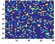
$\theta_{1}$

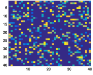
$\theta_{2}$

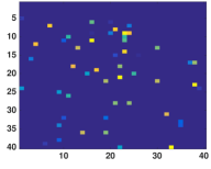
$\delta\theta=\theta_{1}-\theta_{2}$

(a) Sparse Structure

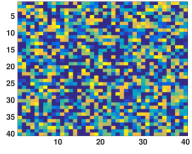
$\theta_{1}$

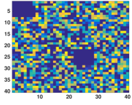
$\theta_{2}$

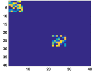
$\delta\theta=\theta_{1}-\theta_{2}$

(b) Group Sparsity Structure

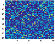
$\theta_{1}$

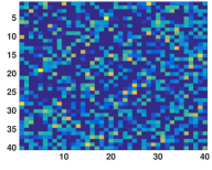
$\theta_{2}$

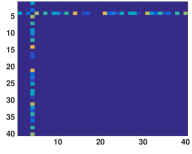
$\delta\theta=\theta_{1}-\theta_{2}$

(c) Node Perturbation Structure

Figure 1: Examples of $\delta\theta$ with different structures. (a) This example shows the sparsity structure of $\delta\theta$, where a few edges has changed between $\theta_{1}$ and $\theta_{2}$. (b) This example presents the group sparsity structure, where a block of edges has changed between $\theta_{1}$ and $\theta_{2}$. (c) This example shows the node perturbation structure, where the connection of one node has changed. Blue represents zeros.

We consider the following optimization problem

$$\underset{{\delta\theta}}{\operatorname{argmin}}~{}~{}{\cal L}(\delta\theta;\mathfrak{X}_{1}^{n_{1}},\mathfrak{X}_{2}^{n_{2}})+\lambda_{n_{1},n_{2}}R(\delta\theta),$$ (1)

where $\mathfrak{X}_{1}^{n_{1}}=\{{\bf{x}}^{1}_{i}\}_{i=1}^{n_{1}}$ and $\mathfrak{X}_{2}^{n_{2}}=\{{\bf{x}}^{2}_{i}\}_{i=1}^{n_{2}}$ are two sets of i.i.d  binary samples drawn from from Ising graphical models with parameter $\theta_{1}^{*}$ and $\theta_{2}^{*}$, respectively, each ${\bf{x}}^{1}_{i}$ and ${\bf{x}}^{2}_{i}$ are $p-$dimensional vectors, and $n_{1},n_{2}$ are the respective sample sizes.

In this Section, we first give a brief background on Ising model selection. Then, we explain how to develop the loss function ${\cal L}(\delta\theta;\mathfrak{X}_{1}^{n_{1}},\mathfrak{X}_{2}^{n_{2}})$ based on the density ratio [9, 10, 25, 31] to directly estimate $\delta\theta=\theta_{1}-\theta_{2}$, and finally we describe how to solve the optimization problem (1) for any norm $R(\delta\theta)$.

2.1 Ising Model

Let $X=(X_{1},X_{2},\cdots,X_{p})$ denote a random vector in which each variable $X_{s}\in\{-1,1\}$. Let $G=(V,E)$ be an undirected graph with vertex set $V=\{1,\cdots,p\}$ and edge set $E$ whose elements are unordered pairs of distinct vertices. The pairwise Ising Markov random field associated with the graph $G$ over the random vector $X$ is

$$P(X={\bf{x}}|\theta^{*}) =\frac{1}{Z(\theta^{*})}\exp\{\sum_{s,t\in E}\theta_{s,t}^{*}x_{s}x_{t}\}$$ (2)

$$=\frac{1}{Z(\theta^{*})}\exp\{\langle\theta^{*},T({\bf{x}})\rangle\}$$ (3)

$$=\frac{1}{Z(\Theta^{*})}\exp\{{\bf{x}}^{T}\Theta^{*}{\bf{x}}\}$$ (4)

where $T({\bf{x}})=\{x_{s}x_{t}\}_{s,t=1}^{p}$ is a vector of size $m=p^{2}$, $\theta^{*}=\{\theta_{s,t}^{*}\}_{s,t=1}^{p}\in\mathbb{R}^{m}$ and $\langle.,.\rangle$ is the inner product operator, and $\Theta^{*}\in\mathbb{R}^{p\times p}$ where $\Theta^{*}_{s,t}=\theta_{s,t}^{*}$. Note that basic Ising models also have non-interacting terms like $\alpha_{s}x_{s}$ and we are assuming these terms are zero, and they do not affect the dependency structure.

The parameter $\theta^{*}$ associated with the structure of the graph $G$ reveals the statistical conditional independence structure among the variables i.e., if $\theta^{*}_{s,t}=0$, then feature $X_{s}$ is conditionally independent of $X_{t}$ given all other variables and there is no edge in the graph $G$.

The partition function, $Z(\theta^{*})$, plays the role of a normalizing constant, ensuring that the probabilities add up to one which is defined as

$$Z(\theta^{*})=\sum_{{\bf{x}}\in\mathcal{X}}\exp\{\langle\theta^{*},T({\bf{x}})\rangle\}=\exp\{\Psi(\theta^{*})\},$$ (5)

where $\mathcal{X}$ be the set of all possible configurations of $X$.

2.2 Loss Function

Here, we build the loss function based on equation (3). Similarly, one can rewrite the loss function based on (4) if the regularization function is over matrices. Consider two Ising models with parameters $\theta_{1}^{*}\in\mathbb{R}^{p^{2}}$ and $\theta_{2}^{*}\in\mathbb{R}^{p^{2}}$. Following Liu et. al [12, 13], a direct estimate for the changes detection problem based on density ratio can be posed as follows

$$r(X={\bf{x}}|\delta\theta)=\frac{p(X={\bf{x}}|\theta_{1})}{p(X={\bf{x}}|\theta_{2})}=\underbrace{\frac{\exp\{\langle T({\bf{x}}),\theta_{1}\rangle\}}{\exp\{\langle T({\bf{x}}),\theta_{2}\rangle\}}}_{r^{*}({\bf{x}}|\delta\theta)}\underbrace{\frac{Z(\theta_{2})}{Z(\theta_{1})}}_{1/Z(\delta\theta)}=\frac{\exp\{\langle T({\bf{x}}),\delta\theta\rangle)\}}{Z(\delta\theta)},$$ (6)

where the parameter $\delta\theta=\theta_{1}-\theta_{2}$ encodes the change between two graphical models $\theta_{1}$ and $\theta_{2}$.

First, we show that $Z(\delta\theta)=E_{X\sim q}[e^{\langle T(X),\delta\theta\rangle}]$:

$$Z(\delta\theta)=\frac{Z(\theta_{1})}{Z(\theta_{2})}=\frac{1}{Z(\theta_{2})}\sum_{{\bf{x}}\in\mathcal{X}}e^{\langle T({\bf{x}}),\theta_{1}\rangle} =\frac{1}{Z(\theta_{2})}\sum_{{\bf{x}}\in\mathcal{X}}e^{\langle T({\bf{x}}),\theta_{2}\rangle}\frac{e^{\langle T({\bf{x}}),\theta_{1}\rangle}}{e^{\langle T({\bf{x}}),\theta_{2}\rangle}}$$

$$=\sum_{{\bf{x}}\in\mathcal{X}}\underbrace{\frac{e^{\langle T({\bf{x}}),\theta_{2}\rangle}}{Z(\theta_{2})}}_{p({\bf{x}}|\theta_{2})}e^{\langle T({\bf{x}}),\delta\theta\rangle}=E_{X\sim p(X|\theta_{2})}[e^{\langle T(X),\delta\theta\rangle}].$$ (7)

Next, using the samples $\mathfrak{X}_{2}^{n_{2}}$ from $p(X|\theta_{2})$, we estimate $Z(\delta\theta)$ empirically as

$$\hat{Z}(\delta\theta)=\frac{1}{n_{2}}\sum_{i=1}^{n_{2}}\exp\{\langle T({\bf{x}}_{i}^{2}),\delta\theta\rangle\},$$ (8)

and the sample approximation of $r(X|\delta\theta)$ is given as

$$\hat{r}(X={\bf{x}}|\delta\theta)=\frac{r^{*}({X=\bf{x}}|\theta_{1})}{\hat{Z}(\delta\theta)}=\frac{\exp\{\langle T({\bf{x}}),\delta\theta\rangle\}}{\frac{1}{n_{2}}\sum_{i=1}^{n_{2}}\exp\{\langle T({\bf{x}}_{i}^{2}),\delta\theta\rangle\}}.$$ (9)

Using the fact that $r(X|\delta\theta^{*})q(X|\theta_{2}^{*})=p(X|\theta_{1}^{*})$, we approximate $\hat{r}(X|\delta\theta)$, by minimizing the $KL$ divergence,

$$KL\left(p(X|\theta_{1}^{*})\|\hat{r}(X|\delta\theta)p(X|\theta_{2}^{*})\right) =\sum_{{\bf{x}}\in\mathcal{X}}p({\bf{x}}|\theta_{1}^{*})\log\frac{p({\bf{x}}|\theta_{1}^{*})}{p({\bf{x}}|\theta_{2}^{*})\hat{r}({\bf{x}}|\delta\theta)}$$

$$=\underbrace{KL\left(p(X|\theta_{1}^{*})\|p(X|\theta_{2}^{*})\right)}_{\text{Constant}}-E_{X\sim p(X|\theta_{1}^{*})}\left[\log\hat{r}(X|\delta\theta)\right]$$ (10)

Thus, using the samples $\mathfrak{X}_{1}^{n_{1}}$ and $\mathfrak{X}_{2}^{n_{2}}$, we define the empirical loss function

$${\cal L}(\delta\theta;\mathfrak{X}_{1}^{n_{1}},\mathfrak{X}_{2}^{n_{2}})=\frac{-1}{n_{1}}\sum_{i=1}^{n_{1}}\log\hat{r}({\bf{x}}_{i}^{1}|\delta\theta)=\frac{-1}{n_{1}}\sum_{i=1}^{n_{1}}\langle T({\bf{x}}_{i}^{1}),\delta\theta\rangle+\underbrace{\log\frac{1}{n_{2}}\sum_{i=1}^{n_{2}}\exp\{\langle T({\bf{x}}_{i}^{2}),\delta\theta\rangle\}}_{\hat{\Psi}(\delta\theta)}$$ (11)

Remark 1

Note that the loss function (11) does not additively decompose over the samples. The second term in (11) is the logarithm over sum of a function of samples.

2.3 Optimization

The optimization problem (1) has a composite objective with a smooth convex term corresponding to the loss function (11) and a a potentially non-smooth convex term corresponding to the regularizer. In this section, we present an algorithm in the class of Fast Iterative Shrinkage-Thresholding Algorithms (FISTA) for efficiently solving the problem (1) [3]. For convenience, we refer the loss function ${\cal L}(\delta\theta;\mathfrak{X}_{1}^{n_{1}},\mathfrak{X}_{2}^{n_{2}})$ as ${\cal L}(\delta\theta)$ and we drop the subscript $\{n_{1},n_{2}\}$ of $\lambda_{n_{1},n_{2}}$.

One of the most popular methods for composite objective functions is in the class of FISTA where at each iteration we linearize the smooth term and minimize the quadratic approximation of the form

$$Q_{L}(\delta\theta,\delta\theta_{t}):={\cal L}(\delta\theta)+\left\langle\delta\theta-\delta\theta_{t},\nabla{\cal L}(\delta\theta_{t})\right\rangle+\frac{L}{2}\|\delta\theta-\delta\theta_{t}\|_{2}^{2}+\lambda R(\delta\theta),$$ (12)

where $L$ denotes the Lipschitz constant of the loss function ${\cal L}(\delta\theta)$. Ignoring constant terms in $\delta\theta_{t}$, the unique minimizer of the above expression (12) can be written as

$$p_{L}(\delta\theta_{t})=\underset{\delta\theta}{\operatorname{argmin}}~{}~{}Q_{{\cal L}}(\delta\theta,\delta\theta_{t}) ~{}=\underset{\delta\theta}{\operatorname{argmin}}~{}~{}\lambda R(\delta\theta)+\frac{L}{2}\left\|\delta\theta-\left(\delta\theta_{t}-\frac{1}{L}\nabla{\cal L}(\delta\theta_{t})\right)\right\|_{2}^{2}$$

$$~{}=\underset{\delta\theta}{\operatorname{argmin}}~{}~{}\frac{\lambda}{L}R(\delta\theta)+\frac{1}{2}\left\|\delta\theta-\left(\delta\theta_{t}-\frac{1}{L}\nabla{\cal L}(\delta\theta_{t})\right)\right\|_{2}^{2}.$$ (13)

In fact, the updates of $\delta\theta$ is to compute certain proximal operators of the non-smooth term $R(.)$. In general, the proximal operator $\text{prox}_{h}({\bf{x}})$ of a closed proper convex function $h:\mathbb{R}^{d}\mapsto\mathbb{R}\cup\{+\infty\}$ [21] is defined as

$$\text{prox}_{h}({\bf{x}})=\underset{{\bf{u}}}{\operatorname{argmin}}\left(h({\bf{u}})+\frac{1}{2}\|{\bf{u}}-{\bf{x}}\|_{2}^{2}\right).$$ (14)

Thus, the unique minimizer (13) correspond to $\text{prox}_{\frac{\lambda}{L}R}\left(\delta\theta_{t}-\frac{1}{L}\nabla{\cal L}(\delta\theta_{t})\right)$ which has rate of convergence of $O(1/t)$ [20, 21].

To improve the rate of convergence, we adapt the idea of FISTA algorithm [3]. The main idea is to iteratively consider the proximal operator $\text{prox}(.)$ at a specific linear combination of the previous two iterates $\{\delta\theta_{t},\delta\theta_{t-1}\}$

$$\xi_{t+1}=\delta\theta_{t}+\alpha_{t+1}\left(\delta\theta_{t}-\delta\theta_{t-1}\right),$$ (15)

instead of just the previous iterate $\delta\theta_{t}$. The choice of $\alpha_{t+1}$ follows Nesterov’s accelerated gradient descent [20, 21] and is detailed in Algorithm 1. The iterative algorithm simply updates

$$\delta\theta_{t+1}=\text{prox}_{\frac{\lambda}{L}R}\left(\xi_{t+1}-\frac{1}{L}\nabla{\cal L}(\xi_{t+1})\right).$$ (16)

The algorithm has a rate of convergence of $O(1/t^{2})$ [3].

Algorithm 1 Generalized Direct Change Estimator

  Input: $L_{0}>0$, $\mathfrak{X}_{1}^{n_{1}},\mathfrak{X}_{2}^{n_{2}}$

  Step 0. Set $\xi_{1}=\delta\theta_{0}$, $t=1$

  Step $t$. ($t\geq 1$) Find the smallest non-negative integers $i_{t}$ such that with $\tilde{L}=2^{i_{t}}L_{t-1}$

$${\cal L}\left(p_{\tilde{L}}(\xi_{t})\right)+R\left(p_{\tilde{L}}(\xi_{t})\right)\leq Q_{\tilde{L}}\left(p_{\tilde{L}}(\xi_{t}),\xi_{t}\right).$$ (17)

  Set $L_{t}=2^{i_{t}}L_{t-1}$ and Compute

$$\delta\theta_{t} =\text{prox}_{\frac{\lambda}{L}R}\left(\xi_{t}-\frac{1}{L}\nabla{\cal L}(\xi_{t})\right)$$ (18)

$$\beta_{t+1} =\frac{1+\sqrt{1+4\beta_{t}^{2}}}{2}$$ (19)

$$\xi_{t+1} =\delta\theta_{t}+\left(\frac{\beta_{t}-1}{\beta_{t+1}}\right)(\delta\theta_{t}-\delta\theta_{t-1})$$ (20)

2.4 Regularization Function

We assume that the optimal $\delta\theta^{*}$ is sparse or suitably ‘structured’ where such structure can be characterized by having a low value according to a suitable norm $R(\delta\theta^{*})$. In below, we provide a few examples of such a norm.

$L_{1}$ norm: One example for $R(.)$ we will consider throughout the paper is the $L_{1}$ norm regularization. We use $L_{1}$ norm if only a few edges has changed (1st row in Figure 1). In particular, we consider $R(\delta\theta)=\|\delta\theta\|_{1}$ if number of non-zeros entries in $\delta\theta^{*}$ is $s<p^{2}$. The $\text{prox}_{\frac{\lambda}{L}\|.\|_{1}}(.)$ is given by the elementwise soft-thresholding operation [24] as

$$\left[\text{prox}_{\frac{\lambda}{L}\|.\|_{1}}\right]_{i}({\bf{z}})={\mbox{\rm sign}}({\bf{z}}_{i}).\max(0,{\bf{z}}_{i}-\frac{\lambda}{L}).$$ (21)

Group-sparse norm: Another popular example we consider is the group-sparse norm. We use group lasso norm if a group of edges has changed (2nd row in Figure 1). For some kinds of data, it is reasonable to assume that the variables can be clustered (or grouped) into types, which share similar connectivity or correlation patterns. Let $\mathcal{G}=\{\mathcal{G}_{1},\mathcal{G}_{2},\cdots,\mathcal{G}_{N_{G}}\}$ denote a collection of groups, which are subsets of variables. We assume that $\delta\Theta^{*}(s,t)=0$ for any variable $s\in G_{g}$ and for any variable $t\in G_{h}$. In the group sparse setting for any subset $S_{\mathcal{G}}\subseteq\{1,2,\cdots N_{G}\}$ with cardinality $|S_{\mathcal{G}}|=s_{\mathcal{G}}$, we assume that the parameter $\delta\Theta^{*}$ satisfies $\{\delta\Theta^{*}_{s,t}=0:s,t\in G_{g}~{}\&~{}g\not\in S_{\mathcal{G}}\}$. We will focus on the case when $R(\delta\Theta)=\sum_{g=1}^{N_{G}}\|\delta\Theta(s,t):s,t\in G_{g}\|_{F}$ [15]. Let $\delta\Theta_{G_{g}}$ bd the sub-matrix of $\delta\Theta$ covering nodes in $G_{g}$. Proximal operator is given by the group specific soft-thresholding operation.

$$\left[\text{prox}_{\frac{\lambda}{L}R}\right]_{g}(\delta\Theta)=\frac{\max(\|\delta\Theta_{G_{g}}\|_{F}-\frac{\lambda}{L},0)}{\|\delta\Theta_{G_{g}}\|_{F}}.$$ (22)

Node perturbation: Another example is the row-column overlap norm (RCON) [18] to capture perturbed nodes i.e., nodes that have a completely different connectivity pattern to other nodes among two networks (3rd row in Figure 1). A special case of RCON we are interested is $\sum_{i=1}^{p}\|V_{i}\|_{q}$ where $\delta\Theta=V+V^{T}$, and $V_{i}$ is the $i-$th column of matrix $V$. This norm can be viewed as overlapping group lasso [18] and thus can be solved by applying Algorithm 1 with proximal operator for overlapping group lasso [35]. Also, we can write problem (1) as a constrained optimization

$$\underset{{\delta\Theta,V}}{\operatorname{argmin}}~{}~{}{\cal L}(\delta\Theta;\mathfrak{X}_{1}^{n_{1}},\mathfrak{X}_{2}^{n_{2}})+\lambda_{1}\delta\Theta\|_{1}+\lambda_{n_{1},n_{2}}\sum_{i=1}^{p}\|V_{i}\|_{q}$$

$$\text{s.t.}\qquad\delta\Theta=V+V^{T},$$ (23)

and solve it by applying in-exact ADMM techniques [18].

3 Statistical Recovery for Generalized Direct Change Estimation

Our goal is to provide non-asymptotic bounds on $\|\Delta\|_{2}=\|\delta\theta^{*}-\delta\hat{\theta}\|_{2}$ between the true parameter $\delta\theta^{*}$ and the minimizer $\delta\hat{\theta}$ of (1). In this section, we describe various aspects of the problem, introducing notations along the way, and highlight our main result.

3.1 Background and Assumption

Gaussian Width: In several of our proofs, we use the concept of Gaussian width [6, 8], which is defined as follows.

Definition 1

For any set $A\in\mathbb{R}^{p}$, the Gaussian width of the set $A$ is defined as:

$$w(A)=E_{g}\left[\sup_{u\in A}\langle g,u\rangle\right]~{}.$$ (24)

where the expectation is over $g\sim N(0,\mathbb{I}_{p\times p})$, a vector of independent zero-mean unit-variance Gaussian random variable.

The Gaussian width $w(A)$ provides a geometric characterization of the size of the set $A$. Consider the Gaussian process $\{Z_{u}\}$ where the constituent Gaussian random variables $Z_{u}=\langle u,g\rangle$ are indexed by $u\in A$, and $g\sim N(0,\mathbb{I}_{p\times p})$. Then the Gaussian width $w(A)$ can be viewed as the expectation of the supremum of the Gaussian process $\{Z_{u}\}$. Bounds on the expectations of Gaussian and other empirical processes have been widely studied in the literature, and we will make use of generic chaining for some of our analysis [4, 11, 29, 30].

The Error Set: Consider solving the problem (1), under assumption $\lambda_{n_{1},n_{2}}>\beta R^{*}\left(\nabla{\cal L}(\delta\theta^{*};\mathfrak{X}_{1}^{n_{1}},\mathfrak{X}_{2}^{n_{2}})\right)$, where $\beta>1$ and $R^{*}(.)$ is the dual norm of $R(.)$. Banerjee et al. [1] show that for any convex loss function the error vector $\Delta=(\delta\theta^{*}-\delta\hat{\theta})$ lies in a restricted set that is characterized as

$$E_{r}=E_{r}(\delta\theta^{*},\beta)=\left\{\Delta\in\mathbb{R}^{p}~{}\left|~{}R(\delta\theta^{*}+\Delta)\leq R(\delta\theta^{*})+\frac{1}{\beta}R(\Delta)\right.\right\}~{}.$$ (25)

Restricted Strong Convexity (RSC) Condition: The sample complexity of the problem (1) depends on the RSC condition [19], which ensures that the estimation problem is strongly convex in the neighborhood of the optimal parameter [1, 19]. A convex loss function satisfies the RSC condition in $C_{r}=cone(E_{r})$, i.e., $\forall\Delta\in C_{r}$, if there exists a suitable constant $\kappa$ such that

$$\delta{\cal L}(\delta\theta^{*},u):={\cal L}(\delta\theta^{*}+u)-{\cal L}(\delta\theta^{*})-\langle\nabla{\cal L}(\delta\theta^{*}),u\rangle\geq\kappa\|u\|_{2}^{2}$$ (26)

Deterministic Recovery Bounds: If the RSC condition is satisfied on the error set $C_{r}$ and $\lambda_{n_{1},n_{2}}$ satisfies the assumptions stated earlier, for any norm $R(.)$, Banerjee et al. [1] show a deterministic upper bound for $\|\Delta\|_{2}$ in terms of $\lambda_{n_{1},n_{2}}$, $\kappa$, and the norm compatibility constant $\Psi(C_{r})=\sup_{\mathbf{u}\in C_{r}}\frac{R(\mathbf{u})}{\|\mathbf{u}\|_{2}}$, as

$$\|\Delta\|_{2}\leq\frac{1+\beta}{\beta}\frac{\lambda_{n_{1},n_{2}}}{\kappa}\Psi(C_{r})~{}.$$ (27)

Smooth Density Ratio Model Assumption: For any vector ${\bf{u}}$ such that $\|{\bf{u}}\|_{2}\leq\|\delta\theta^{*}\|_{2}$ and every $\epsilon\in R$, the following inequality holds:

$$E_{X\sim p(X|\theta_{2})}[\exp\{\epsilon~{}r(X|\delta\theta^{*}+{\bf{u}})-1\}]\leq\exp\{\epsilon^{2}\}.$$

A similar assumption is used in the analysis of Liu et al. [13].

Remark 2

Bounded density ratio is a special case satisfying the smooth density ratio assumption. Lemma 1 shows a sufficient condition under which the density ratio is bounded.

Lemma 1

Consider two Ising Model with true parameters $\theta_{1}^{*}$ and $\theta_{2}^{*}$. Let $d_{1},d_{2}\gg s$ where $\|\theta_{1}^{*}\|_{0}=d_{1}$, $\|\theta_{2}^{*}\|_{0}=d_{2}$, and $\|\delta\theta^{*}\|_{0}=s$. Assume

$$\min_{i,j=1\cdots p}(|\theta_{1}^{*}(i,j)|) \geq\frac{1}{d_{1}-1}-\frac{c_{1}}{(d_{1}-1)s}$$ (28)

$$\min_{i,j=1\cdots p}(|\theta_{2}^{*}(i,j)|) \geq\frac{1}{d_{2}-1}-\frac{c_{2}}{(d_{2}-1)s},$$ (29)

where $c_{1}$ and $c_{2}$ are positive constants. Then the density ratio $r(X={\bf{x}}|\delta\theta^{*})$ is bounded.

Note that if individual graphs are dense, then the conditions (28) and (29) are satisfied and as a result the smooth density ratio is satisfied.

Remark 3

In this paper, we focus on the Ising graphical model. But, our statistical analysis holds for any graphical models that satisfy the above mentioned assumption. Through our analysis, no assumption is required on the individual graphical models.

3.2 Bounds on the regularization parameter

To get the recovery bound (27) above, one needs to have $\lambda_{n_{1},n_{2}}\geq\beta R^{*}\left(\nabla{\cal L}(\delta\theta^{*};\mathfrak{X}_{1}^{n_{1}},\mathfrak{X}_{2}^{n_{2}})\right)$. However, the bound on $\lambda_{n_{1},n_{2}}$ depends on unknown quantity $\delta\theta^{*}$ and the samples $\mathfrak{X}_{1}^{n_{1}},\mathfrak{X}_{2}^{n_{2}}$ and is hence random. To overcome the above challenges, one can bound the expectation $E[R^{*}\left(\nabla{\cal L}(\delta\theta^{*};\mathfrak{X}_{1}^{n_{1}},\mathfrak{X}_{2}^{n_{2}})\right)]$ over all samples of size $n_{1}$ and $n_{2}$, and obtain high-probability deviation bounds. The goal is to provide a sharp bound on $\lambda_{n_{1},n_{2}}$ since the error bound in (27) is directly proportional to $\lambda_{n_{1},n_{2}}$.

In theorem 1, we characterize the expectation $E[R^{*}\left(\nabla{\cal L}(\delta\theta^{*};\mathfrak{X}_{1}^{n_{1}},\mathfrak{X}_{2}^{n_{2}})\right)]$ in terms of the Gaussian width of the unit norm-ball of $R(.)$, which leads to a sharp bound. The upper bound on Gaussian width of the unit norm-ball of $R$ for atomic norms which covers a wide range of norms is provided in [6, 7].

Theorem 1

Define $\Omega_{R}=\{u:R(u)\leq 1\}$. Let $\phi(R)=\sup_{{\bf{u}}}\frac{\|{\bf{u}}\|_{2}}{R({\bf{u}})}$. Assume that for any ${\bf{u}}$ that $\|{\bf{u}}\|\leq\|\theta^{*}\|$

$$\frac{1}{2}\lambda_{\max}\left(\nabla^{2}{{\cal L}}(\delta\theta^{*}+{{\bf{u}}})\right)\leq\eta_{0},$$ (30)

where $\lambda_{\max}(.)$ is the maximum eigenvalue. Then under the smooth density ratio assumption, we have

$$E\left[R^{*}(\nabla{\cal L}(\delta\theta^{*};\mathfrak{X}_{1}^{n_{1}},\mathfrak{X}_{2}^{n_{2}}))\right]\leq\frac{2\sqrt{\eta_{0}}(c_{1}w\left(\Omega_{R})+\phi(R)\right)}{\sqrt{\min(n_{1},n_{2})}}.$$

and with probability at least $1-c_{2}e^{-\epsilon^{2}}$

$$R^{*}\left(\nabla{\cal L}(\delta\theta^{*};\mathfrak{X}_{1}^{n_{1}},\mathfrak{X}_{2}^{n_{2}})\right)\leq\frac{c_{2}(1+\epsilon)w(\Omega_{R})+\tau_{1}}{\sqrt{\min(n_{1},n_{2})}}.$$

where $c_{1}$ and $c_{2}$ are positive constants, $\tau_{1}=2\sqrt{\eta_{0}}\phi(R)$, and $w(\Omega_{R})$ is the Gaussian width of set $\Omega_{R}$.

Note, that our analysis hold for any norm and it is expressed in terms of the Gaussian width. In the following, we give the bound on the regularization parameter for two examples of the regularization function $R(.)$.

Corollary 1

If $R(\delta\theta)$ is the $L_{1}$ norm, and $\delta\theta\in\mathbb{R}^{p^{2}}$ then with high probability we have the bound

$$R^{*}\left(\nabla{\cal L}(\delta\theta^{*};\mathfrak{X}_{1}^{n_{1}},\mathfrak{X}_{2}^{n_{2}})\right)\leq\frac{\eta_{2}\sqrt{\log p}}{\sqrt{\min(n_{1},n_{2})}}.$$ (31)

Corollary 2

If $R(\delta\theta)$ is the group-sparse norm, and $\delta\theta\in\mathbb{R}^{p^{2}}$ then with high probability we have the bound

$$R^{*}\left(\nabla{\cal L}(\delta\theta^{*};\mathfrak{X}_{1}^{n_{1}},\mathfrak{X}_{2}^{n_{2}})\right)\leq\frac{\eta_{2}\sqrt{m+\log N_{G}}}{\sqrt{\min(n_{1},n_{2})}},$$ (32)

where $\mathcal{G}=\{\mathcal{G}_{1},\cdots,\mathcal{G}_{N_{G}}\}$ is a collection of groups, $m=\max_{i}|\mathcal{G}_{i}|$ is the maximum size of any group.

3.3 RSC Condition

In this Section, we establish the RSC condition for direct change detection estimator (1). Simplifying the expression and applying mean value theorem twice on the left side of RSC condition (26), for $\forall\gamma_{i}\in[0,1]$, we have

$$\delta{\cal L}(\delta\theta^{*},u):={\cal L}(\delta\theta^{*}+u)-{\cal L}(\delta\theta^{*})-\langle\nabla{\cal L}(\delta\theta^{*}),u\rangle\geq u^{T}\nabla^{2}{\cal L}(\delta\theta^{*}+\gamma_{i}u)u.$$ (33)

Thus, the RSC condition depends on the non-linear terms of loss function. Recall that the nonlinear term, second term, in Loss function (1) which is the approximation of the log-partition functions only depends on $n_{2}$. As a results, only samples of $\mathfrak{X}_{2}^{n_{2}}$ affect the RSC conditions. Our analysis is an extension of the results on [1] using the generic chaining. We show that, with high probability the RSC condition is satisfied once samples $n_{2}$ crosses $w^{2}(C_{r}\cap S^{d-1})$ the Gaussian width of restricted error set. The bound on Gaussian width of the error set for atomic norms has been provided in [7].

Let $r_{i}=r(X={\bf{x}_{i}^{2}}|\delta\theta^{*})$ and $\bar{\varepsilon}$ denote the probability that $r_{i}$ exceeds some constant $\eta_{0}$: $\bar{\varepsilon}=p(r_{i}>\eta_{0})\geq 1-e^{-\frac{\eta_{0}^{2}}{2}}$.

Theorem 2

Let $X\in\mathbb{R}^{n\times p}$ be a design matrix with independent isotropic sub-Gaussian rows with ${\left|\kern-1.07639pt\left|\kern-1.07639pt\left|X_{i}\right|\kern-1.07639pt\right|\kern-1.07639pt\right|}_{\Psi_{2}}\leq\kappa$. Then, for any set $A\subseteq S^{p-1}$, for suitable constants $\eta$, $c_{1}$, $c_{2}>0$ with probability at least $1-\exp(-\eta w^{2}(A))$, we have

$$\inf_{u\in A}\partial{\cal L}(\theta^{*};u,X)\geq c_{1}\underline{\rho}^{2}\left(1-c_{2}\kappa_{1}^{2}\frac{w(A)}{\sqrt{n_{2}}}\right)-\tau$$ (34)

where $\kappa_{1}=\frac{\kappa}{\bar{\varepsilon}}$, $\underline{\rho}^{2}=\inf_{{\bf{u}}\in A}\rho_{\bf{u}}^{2}$ with $\rho_{\bf{u}}^{2}=E\left[\left\langle{\bf{u}},T(X_{i}^{2})\right\rangle^{2}\mathbb{I}(r_{i}>\eta_{0})\right]$, and $\tau$ is smaller than the first term in right hand side. Thus, for $n_{2}\geq c_{2}w^{2}(A)$, with probability at least $1-\exp(-\eta w^{2}(A))$, we have $\inf_{u\in A}\partial{\cal L}(\theta^{*};u,X)>0$.

3.4 Statistical Recovery

With the above results in place, from (27), Theorem 3 provides the main recovery bound for generalized direct change estimator (1).

Theorem 3

Consider two set of i.i.d samples $\mathfrak{X}_{1}^{n_{1}}=\{{\bf{x}}^{1}_{i}\}_{i=1}^{n_{1}}$ and $\mathfrak{X}_{2}^{n_{2}}=\{{\bf{x}}^{2}_{i}\}_{i=1}^{n_{2}}$. Define $\Omega_{R}=\{u:R(u)\leq 1\}$. Assume that $\delta\hat{\theta}$ is the minimizer of the problem (1). Then, with probability at least $1-\eta_{0}e^{-\epsilon^{2}}$ the followings hold

$$\lambda_{n_{1},n_{2}}\geq\frac{\eta_{1}}{\sqrt{\min(n_{1},n_{2})}}(w(\Omega_{R})+\epsilon)$$ (35)

and for $n_{2}\geq cw^{2}(C_{r}\cap S^{d-1})$, with high probability, the estimate $\delta\hat{\theta}$ satisfies

$$\|\Delta\|_{2}\leq O\left(\frac{w(\Omega_{R})}{\sqrt{\min(n_{1},n_{2})}}\right)\Psi(C_{r})~{},$$ (36)

where $w(.)$ is the Gaussian width of a set,and $c_{2}$, $\eta_{0}$, and $\eta_{1}$ are positive constants.

Proof.

Proof of the Theorem can be directly obtain as the results of (27) and Theorem 1 and Theorem 2.

In the following, we provide the recovery bound for two special cases as an example.

Corollary 3

If $R(\delta\theta)$ is the $L_{1}$ norm, $\delta\theta^{*}\in\mathbb{R}^{p^{2}}$ s $s$-sparse., $\Psi(C_{r})\leq 4\sqrt{s}$, and for $n_{2}>cs\log p$, the recovery error is bounded by

$$\|\Delta\|_{2}\leq c_{3}\frac{\Psi(C_{r})\lambda_{n_{1},n_{2}}}{\kappa}=O\left(\sqrt{\frac{s\log p}{\min(n_{1},n_{2})}}\right).$$

Corollary 4

If $R(\delta\theta)$ is the group-sparse norm, $\delta\theta\in\mathbb{R}^{p^{2}}$, $\Psi(C_{r})\leq 4\sqrt{s_{G}}$ and for $n_{2}\geq c(ms_{G}+s_{G}\log N_{G})$, the recovery error is bounded by

$$\|{\Delta}\|_{2} \leq c_{3}\frac{\Psi(C_{r})\lambda_{n_{1},n_{2}}}{\kappa}=O\left(\sqrt{\frac{s_{G}m+\log N_{G}}{\min(n_{1},n_{2})}}\right).$$

4 Experiments

In this Section, we evaluate generalized direct change estimator (direct) with three different norms. and we compare our direct approach with indirect approach. For indirect approach, we first estimate Ising model structures $\hat{\theta}_{1}$ and $\hat{\theta}_{2}$ with $L_{1}$ norm regularizer, separately [22]. Then, we obtain $\delta\hat{\theta}=\hat{\theta}_{1}-\hat{\theta}_{2}$. In all experiments, we draw $n_{1}$ and $n_{2}$ i.i.d samples from each Ising model by running Gibbs sampling. Here we set $n=n_{1}=n_{2}=\{20,50,100\}$.

$L_{1}$ norm: Here we first generate $\theta_{1}^{*}$ with three disconnected star sub-graphs (Figure 1-a) with $p=50$. We generate the weights uniformly random between $\{0.3-0.5\}$. We then generate $\theta_{2}^{*}$ by removing 10 random edges from $\theta_{1}^{*}$ (Figure 1-b). It is interesting that although individual graphs are sparse, but direct approach has a better ROC curve for all values of $n$ (Figure 1-d). Similar results obtained by with random graph structure of $\theta_{1}^{*}$ and $\theta_{2}^{*}$.

Group-sparse norm: In this set of experiments, we evaluate direct method with three different structure for $\theta_{1}^{*}$: (i) a random graph structure (Figure 1-e), (ii) scale free graph structure (Figure 1-i), and (iii) a cluster graph structure (Figure 1-m). In all settings, we set $p=60$ and generate $\theta_{2}^{*}$ by removing a block of edges from $\theta_{1}^{*}$ (Figure 1-(f,j,n)). For random graph structure and block structure, direct method has a better ROC curve (Figure 1-h,p). But, for scale-free structure, since the individual graphs are sparse, indirect method can estimate $\hat{\theta}_{1}$ and $\hat{\theta}_{2}$ correctly, and thus have a better ROC curve (Figure 1-l).

Node perturbation: Here, we first generate a random graph structure $\theta_{1}^{*}$, and then generate $\theta_{2}^{*}$ by perturbing two nodes in $\theta_{1}^{*}$. Here we set $p=60$ and generate $\theta_{2}^{*}$ by setting rows and columns $3,51$ to zero in $\theta_{1}^{*}$ (Figure 1-s). Although, the individual graphs are dense but direct approach can estimate edges in $\delta\theta$ with only $n=20$ samples (Figure 1-t).

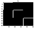
$\theta_{1}$

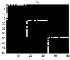
$\theta_{2}$

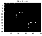
$\delta\theta=\theta_{1}-\theta_{2}$

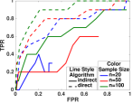
ROC

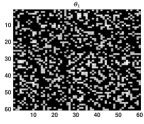
$\theta_{1}$

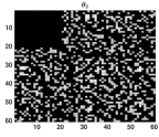
$\theta_{2}$

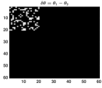
$\delta\theta=\theta_{1}-\theta_{2}$

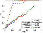
ROC

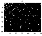
$\theta_{1}$, scale-free

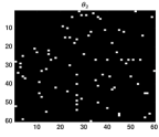
$\theta_{2}$

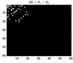
$\delta\theta=\theta_{1}-\theta_{2}$

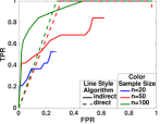
ROC

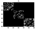
$\theta_{1}$

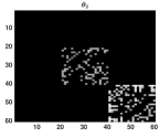
$\theta_{2}$

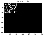
$\delta\theta=\theta_{1}-\theta_{2}$

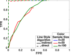
ROC

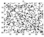
$\theta_{1}$

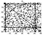
$\theta_{2}$

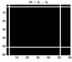
$\delta\theta=\theta_{1}-\theta_{2}$

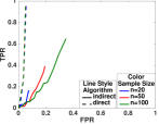
ROC

Figure 2: First row $\delta\theta^{*}$ has a sparse structure ($L_{1}$ norm) and $\theta_{1}^{*}$ has 3 disconnected star graphs. Second, third, and forth rows $\delta\theta^{*}$ has group sparse structure (group sparse norm) where $\theta_{1}^{*}$ has a random graph structure in second row, scale-free structure in third row, and block structure in forth row. Last row $\delta\theta^{*}$ has two perturbed norm (Node perturbation) and $\theta_{1}^{*}$ has a random graph structure. Blacks in heatmaps denotes zeros. ROC curve for different structures show in the last column. Direct approach has a better ROC curve for all structures except with scale-free structure of $\theta_{1}^{*}$.

5 Conclusion

This paper presents the statistical analysis of direct change problem in Ising graphical models where any norm can be plugged in for characterizing the parameter structure. An optimization algorithm based on FISTA-style algorithms is proposed with the convergence rate of $O(1/T^{2})$. We provide the statistical analysis for any norm such as $L_{1}$ norm, group sparse norm, node perturbation, etc. Our analysis is based on generic chaining and illustrates the important role of Gaussian widths (a geometric measure of size of suitable sets) in such results. For the special case of sparsity, we obtain a sharper result than previous results [13] under the same smooth density ratio assumption. Liu et al. [13] obtained the same result with a bounded density ratio assumption which is a more restrictive assumption. Although, we presented the results for Ising model, our analysis can be applied to any graphical model which satisfies the smooth density ratio assumption. Further, we extensively compared our generalized direct change estimator with an indirect approach over a wide range of graph structures and norms. We show that our direct approach has a better ROC curve than indirect approach without any assumption on the structure of individual graphs. We implemented indirect approach by estimating individual Ising model structures with $L_{1}$ norm regularizer. However, if individual graphs has a suitable structure such as group sparsity, one may apply a regularization that can characterize the graph structure and may improve performance of the indirect approach. We will investigate this possibility in our future research.

Appendix

Appendix A Background and Preliminaries

Definition 2

Sub-Gaussian random variable: We say that a random variable $x$ is sub-Gaussian if the moments satisfies

$$[E|x|^{p}]^{\frac{1}{p}}\leq K_{2}\sqrt{p}$$ (37)

for any $p\geq 1$ with a constant $K_{2}$. The minimum value of $K_{2}$ is called sub-Gaussian norm of $x$, denoted by ${\left|\kern-1.07639pt\left|\kern-1.07639pt\left|x\right|\kern-1.07639pt\right|\kern-1.07639pt\right|}_{\psi_{2}}$. If $E[x]=0$, then

$$E[\exp\{tX\}]\leq\exp\{Ct^{2}{\left|\kern-1.07639pt\left|\kern-1.07639pt\left|X\right|\kern-1.07639pt\right|\kern-1.07639pt\right|}_{\Psi_{2}}^{2}\},$$ (38)

where $C$ and $c$ are positive constant.

Definition 3

Sub-Gaussian random vector: We say that a random vector $X$ in $\mathbb{R}^{n}$ is sub-Gaussian if the one-dimensional marginals $\langle X,{\bf{x}}\rangle$ are sub-Gaussian random variables for all ${\bf{x}}\in\mathbb{R}^{n}$. The sub-Gaussian norm of $X$ is defined as

$${\left|\kern-1.07639pt\left|\kern-1.07639pt\left|X\right|\kern-1.07639pt\right|\kern-1.07639pt\right|}_{\psi_{2}} =\sup\limits_{{\bf{x}}\in S^{n-1}}\|\langle X,{\bf{x}}\rangle\|_{\psi_{2}}$$ (39)

Lemma 2

Consider a sub-Gaussian vector $X\in\mathbb{R}^{n}$ with ${\left|\kern-1.07639pt\left|\kern-1.07639pt\left|X\right|\kern-1.07639pt\right|\kern-1.07639pt\right|}_{\Psi_{2}}<K$, then for any vector $u$, $\langle X,u\rangle$ is a sub-Gaussian variable with ${\left|\kern-1.07639pt\left|\kern-1.07639pt\left|\langle X,u\rangle\right|\kern-1.07639pt\right|\kern-1.07639pt\right|}<K\|u\|_{2}$.

Proof.

The argument is based on Definition 3 as follows,

$${\left|\kern-1.07639pt\left|\kern-1.07639pt\left|\langle X,u\rangle\right|\kern-1.07639pt\right|\kern-1.07639pt\right|}_{\Psi_{2}}=\|u\|_{2}{\left|\kern-1.07639pt\left|\kern-1.07639pt\left|\left\langle X,\frac{u}{\|u\|_{2}}\right\rangle\right|\kern-1.07639pt\right|\kern-1.07639pt\right|}_{\Psi_{2}}\leq\|u\|_{2}\sup_{x\in S^{n-1}}\langle X,x\rangle=\|u\|_{2}{\left|\kern-1.07639pt\left|\kern-1.07639pt\left|X\right|\kern-1.07639pt\right|\kern-1.07639pt\right|}_{\Psi_{2}}\leq K\|u\|_{2}.$$ (40)

∎

Lemma 3

Let $X_{1}$ and $X_{2}$ be centered sub-Gaussian random variables with ${\left|\kern-1.07639pt\left|\kern-1.07639pt\left|X_{1}\right|\kern-1.07639pt\right|\kern-1.07639pt\right|}_{\Psi_{2}}=b_{1}$ and ${\left|\kern-1.07639pt\left|\kern-1.07639pt\left|X_{2}\right|\kern-1.07639pt\right|\kern-1.07639pt\right|}_{\Psi_{1}}=b_{2}$. Then $X_{1}+X_{2}$ is centered sub-Gaussian with ${\left|\kern-1.07639pt\left|\kern-1.07639pt\left|X_{1}+X_{2}\right|\kern-1.07639pt\right|\kern-1.07639pt\right|}_{\Psi_{2}}=b_{1}+b_{2}$.

Proof.

The argument is based on the definition of moment generating function of sub-Gaussian random variable:

Using Holder inequality for any $p,q>0$ where $\frac{1}{p}+\frac{1}{q}=1$, we have

$$E[\exp\{t(X_{1}+X_{2})\}] \leq(E[\exp\{tX_{1}\}^{p}])^{1/p}(E[\exp\{tX_{1}\}^{q}])^{1/q}$$

$$\leq\exp\{Ct^{2}(pb_{1}^{2}+qb_{2}^{2})\}=\exp\{Ct^{2}(pb_{1}^{2}+\frac{p}{1-p}b_{2}^{2})\}.$$ (41)

The minimum of (41) occurs with $p=\frac{b_{2}}{b_{1}}$. As a result, we have

$$E[\exp\{t(X_{1}+X_{2})\}]\leq\exp\{Ct^{2}(b_{1}+b_{2})^{2}\}.$$ (42)

The proof is complete. ∎

A.1 Generic Chaining

Definition 4 (Majorizing measure [27])

Given $\alpha>0$, and a metric space $(T,d)$ (that need not be finite), we define

$$\gamma_{\alpha}(T,d)=\inf\sup_{t}\sum_{n\geq 0}2^{n/\alpha}\Delta(A_{n}(T)).$$ (43)

where the infimum is taken over all admissible sequences and $\Delta(A_{n}(T))$ is the diameter of $A_{n}(t)$.

Note that $\gamma_{2}(T,\|.\|_{2})$ coincides with the Gaussian width of $T$: $w(T)$.

Lemma 4

Given a metric space $(T,d)$, we have

$$\gamma_{1}(T,\|.\|_{\infty})\leq\gamma_{2}^{2}(T,\|.\|_{2}).$$ (44)

Proof.

Define $d_{2}(s,t)=\|s-t\|_{2}$ and $d_{1}(s,t)=\|s-t\|_{\infty}$. We use the traditional definition of majorizing measure $\gamma_{\alpha,1}(T,d)$ from [27]

$$\gamma_{\alpha,1}(T,d)=\inf\sup_{t}\left(\int_{0}^{\infty}\left(\log\frac{1}{\mu(B_{d}(t,\varepsilon))}\right)^{1/\alpha}d\varepsilon\right).$$ (45)

where $B_{d}(t,\varepsilon)$ is the closed ball of center $t$ and radius $\varepsilon$ based on the distance $d$ and the infimum is taken over all the probability measure $\mu$ on $T$.

Note that $\gamma_{\alpha,1}(T,d)$ coincides with the functional $\gamma_{\alpha}(T,d)$ [28] as

$$K(\alpha)^{-1}\gamma_{\alpha}(T,d)\leq\gamma_{\alpha,1}(T,d)\leq K(\alpha)\gamma_{\alpha}(T,d),$$ (46)

where $K(\alpha)$ is a constant depending on $\alpha$ only.

As a result, it is enough to show that $\gamma_{1,1}(T,d_{1})\leq\gamma_{2,1}^{2}(T,d_{2})$.

Note that since for any vector $x$, we have $\|x\|_{\infty}\leq\|x\|_{2}$, therefore, for any probability measure $\mu$ and $t$, we have $\mu(B_{d_{1}}(t,\varepsilon))\geq\mu(B_{d_{2}}(t,\varepsilon))$. As a result,

$$\left(\int_{0}^{\infty}\left(\log\frac{1}{\mu(B_{d_{1}}(t,\varepsilon))}\right)d\varepsilon\right)\leq\left(\int_{0}^{\infty}\left(\log\frac{1}{\mu(B_{d_{2}}(t,\varepsilon))}\right)d\varepsilon\right)\leq\left(\int_{0}^{\infty}\left(\log\frac{1}{\mu(B_{d_{2}}(t,\varepsilon))}\right)^{1/2}d\varepsilon\right)^{2}.$$ (47)

Since (47) holds for any $\mu$ and $t$, we have

$$\gamma_{1,1}(T,d_{1})=\inf\sup_{t}\left(\int_{0}^{\infty}\left(\log\frac{1}{\mu(B_{d_{1}}(t,\varepsilon))}\right)d\varepsilon\right) \leq\inf\sup_{t}\left(\int_{0}^{\infty}\left(\log\frac{1}{\mu(B_{d_{2}}(t,\varepsilon))}\right)^{1/2}d\varepsilon\right)^{2}$$

$$=\gamma^{2}_{2,1}(T,d_{2}).$$ (48)

This completes the proof. ∎

Theorem 4

[Theorem 1.2.7] in [29] Consider a set $T$ provided with two distances $d_{1}$ and $d_{2}$. Consider a process $(X_{t})_{t\in T}$ that satisfies $E[X_{t}]=0$ and

$$P\left(|X_{s}-X_{t}|\geq u\right)\leq 2\exp\left(-\min\left(\frac{u^{2}}{d_{2}(s,t)^{2}},\frac{u}{d_{1}(s,t)}\right)\right).$$ (49)

Then

$$E[\sup_{t,s\in T}|X_{s}-X_{t}|\leq L(\gamma_{1}(T,d_{1})+\gamma_{2}(T,d_{2})),$$ (50)

where $L$ is a constant.

Theorem 5

[Theorem 1.2.9] in [29] Under the conditions of Theorem 4, for all values of $u_{1},u_{2}>0$ we have

$$P\left(|X_{s}-X_{t0}|\geq L(\gamma_{1}(T,d_{1})+\gamma_{2}(T,d_{2}))+u_{1}D_{1}+u_{2}D_{2}\right)$$

$$\qquad\leq L\exp(-\min(u_{2}^{2},u_{1})),$$ (51)

where $D_{j}=2\sum_{n\geq 0}e_{n}(T,d_{j})$. Note that $D_{j}\leq L\gamma_{j}(T,d_{j})$.

Theorem 6

[Theorem 8.2 (Fernique-Talagrand’s comparison theorem)] in [32] Let $T$ be an arbitrary set. Consider a Gaussian random process $(G(t))_{t\in T}$ and a sub-Gaussian random process $(H(t))_{t\in T}$. Assume that $E[G(t)]=E[H(t)]=0$ for all $t\in T$. Assume also that for some $M>0$, the following increment comparison holds:

$${\left|\kern-1.07639pt\left|\kern-1.07639pt\left|H(s)-H(t)\right|\kern-1.07639pt\right|\kern-1.07639pt\right|}_{\psi_{2}}\leq M(E[\|G(s)-G(t)\|_{2}^{2})^{1/2}\qquad\forall s,t\in T.$$ (52)

Then

$$E[sup_{t\in T}H(t)]\leq CME[sup_{t\in T}G(t)].$$ (53)

Theorem 7 (Mendelson, Pajor, Tomczak-Jaegermann [17])

There exist absolute constants $c_{1}$, $c_{2}$, $c_{3}$ for which the following holds. Let $(\Omega,\mu)$ be a probability space, set $F$ be a subset of the unit sphere of $L_{2}(\mu)$, i.e., $F\subseteq S_{L_{2}}=\{f:{\left|\kern-1.07639pt\left|\kern-1.07639pt\left|f\right|\kern-1.07639pt\right|\kern-1.07639pt\right|}_{L_{2}}=1\}$, and assume that $\sup_{f\in F}~{}{\left|\kern-1.07639pt\left|\kern-1.07639pt\left|f\right|\kern-1.07639pt\right|\kern-1.07639pt\right|}_{\psi_{2}}\leq\kappa$. Then, for any $\theta>0$ and $n\geq 1$ satisfying

$$c_{1}\kappa\gamma_{2}(F,{\left|\kern-1.07639pt\left|\kern-1.07639pt\left|\cdot\right|\kern-1.07639pt\right|\kern-1.07639pt\right|}_{\psi_{2}})\leq\theta\sqrt{n}~{},$$ (54)

with probability at least $1-\exp(-c_{2}\theta^{2}n/\kappa^{4})$,

$$\sup_{f\in F}~{}\left|\frac{1}{n}\sum_{i=1}^{n}f^{2}(X_{i})-E\left[f^{2}\right]\right|\leq\theta~{}.$$ (55)

Further, if $F$ is symmetric, then

$$E\left[\sup_{f\in F}~{}\left|\frac{1}{n}\sum_{i=1}^{n}f^{2}(X_{i})-E\left[f^{2}\right]\right|\right]\leq c_{3}\max\left\{2\kappa\frac{\gamma_{2}(F,{\left|\kern-1.07639pt\left|\kern-1.07639pt\left|\cdot\right|\kern-1.07639pt\right|\kern-1.07639pt\right|}_{\psi_{2}})}{\sqrt{n}},\frac{\gamma_{2}^{2}(F,{\left|\kern-1.07639pt\left|\kern-1.07639pt\left|\cdot\right|\kern-1.07639pt\right|\kern-1.07639pt\right|}_{\psi_{2}})}{n}\right\}$$ (56)

Appendix B Regularization Parameter

Lemma 5

Consider two Ising Model with true parameters $\theta_{1}^{*}$ and $\theta_{2}^{*}$. Let $d_{1},d_{2}\gg s$ where $\|\theta_{1}^{*}\|_{0}=d_{1}$, $\|\theta_{2}^{*}\|_{0}=d_{2}$, and $\|\delta\theta^{*}\|_{0}=s$. Assume

$$\min_{i,j=1\cdots n_{1}}(|\theta_{1}^{*}(i,j)|) \geq\frac{1}{d_{1}-1}-\frac{c_{1}}{(d_{1}-1)s}$$ (57)

$$\min_{i,j=1\cdots n_{2}}(|\theta_{2}^{*}(i,j)|) \geq\frac{1}{d_{2}-1}-\frac{c_{2}}{(d_{2}-1)s},$$ (58)

where $c_{1}$ and $c_{2}$ are positive constants. Then the density ratio $r(X={\bf{x}}|\delta\theta^{*})$ is bounded.

Proof.

Let $\alpha_{1}\leq|\theta_{1}^{*}|\leq\beta_{1}$ and $\alpha_{2}\leq|\theta_{2}^{*}|\leq\beta_{2}$. Without loss of generality, assume that $\|\theta_{1}^{*}\|_{2}=1$ and $\|\theta_{2}^{*}\|_{2}=1$.

So,

$$\beta_{1} \leq 1-(d_{1}-1)\alpha_{1}$$ (59)

$$\beta_{2} \leq 1-(d_{2}-1)\alpha_{2}.$$ (60)

Based on triangle inequality of norms, we have

$$\|\delta\theta^{*}\|_{\infty}=\|\theta_{1}^{*}-\theta_{2}^{*}\|_{\infty}\leq\|\theta_{1}^{*}\|_{\infty}+\|\theta_{2}^{*}\|_{\infty}\leq\beta_{1}+\beta_{2}\leq 2-(d_{1}-1)\alpha_{1}-(d_{2}-1)\alpha_{2}.$$ (61)

Let ${\bf{z}}=T({\bf{x}})$, then,

$$|\langle{\bf{z}},\delta\theta^{*}\rangle| \leq\|{\bf{z}}\|_{\infty}\|\delta\theta^{*}\|_{1}$$ (62)

$$\leq s\|\delta\theta^{*}\|_{\infty}$$ (63)

$$\leq 2s-[(d_{1}-1)\alpha_{1}-(d_{2}-1)\alpha_{2}]s$$ (64)

where the second inequality is the result of $\|{\bf{z}}\|_{\infty}\leq 1$ since ${\bf{z}}$ comes from an Ising model.

Note that if

$$\alpha_{1}\geq\frac{s-c_{1}}{(d_{1}-1)s}=\frac{1}{d_{1}-1}-\frac{c_{1}}{(d_{1}-1)s},$$ (65)

then

$$s-(d_{1}-1)\alpha_{1}s\leq c_{1}.$$ (66)

Similarly, if

$$\alpha_{2}\geq\frac{s-c_{2}}{(d_{2}-1)s}=\frac{1}{d_{2}-1}-\frac{c_{2}}{(d_{2}-1)s},$$ (67)

then

$$s-(d_{2}-1)\alpha_{2}s\leq c_{2}.$$ (68)

As a result, we have

$$|\langle{\bf{z}},\delta\theta^{*}\rangle|\leq c_{1}+c_{2}.$$ (69)

$$\Rightarrow \exp\{\langle{\bf{z}},\delta\theta^{*}\rangle\}\leq\exp{c_{1}+c_{2}}\leq c_{0}.$$ (70)

For example, if $c_{1}=c_{2}=1$, then $c_{0}=10$.

Therefore,

$$r(X={\bf{x}}|\delta\theta)=\frac{\exp\{\langle{\bf{z}},\delta\theta\rangle)\}}{Z(\delta\theta^{*})}\leq\frac{c_{0}}{Z(\delta\theta^{*})}.$$ (71)

This completes the proof. ∎

Assumption 1(Smooth Density Ratio Model Assumption) For any vector ${\bf{u}}$ such that $\|{\bf{u}}\|_{2}\leq\|\delta\theta^{*}\|_{2}$ and every $t\in R$, the following inequality holds:

$$E_{X\sim p(X|\theta_{2})}[\exp\{tr(X|\delta\theta^{*}+{\bf{u}})-1\}]\leq\exp\{t^{2}\}.$$ (72)

Lemma 6

For any constant $\tau\leq 1$, define random event $M_{\tau}$ as follows,

$$M_{\tau}=\{\Psi(\delta\theta^{*}+{\bf{u}})-\Psi(\delta\theta^{*})-\left[\hat{\Psi}(\delta\theta^{*}+{\bf{u}})-\hat{\Psi}(\delta\theta^{*})\right]\leq\tau\}.$$ (73)

Then, for any vector ${\bf{u}}$ such that $\|{\bf{u}}\|_{2}\leq\|\delta\theta^{*}\|_{2}$, under Assumption 1, we have

$$P(M_{\tau}^{c})=p\left(\Psi(\delta\theta^{*}+{\bf{u}})-\Psi(\delta\theta^{*})-\left[\hat{\Psi}(\delta\theta^{*}+{\bf{u}})-\hat{\Psi}(\delta\theta^{*})\right]>\tau\right)\leq 4e^{-\frac{n_{2}}{5}\tau^{2}}.$$ (74)

Proof.

Recall that

$$r(X={\bf{x}}|\delta\theta^{*})=\frac{\exp\{\langle T({\bf{x}}),\delta\theta^{*}\rangle\}}{Z(\delta\theta^{*})}$$

$$\Rightarrow \qquad\hat{Z}(\delta\theta^{*})=\frac{1}{n_{2}}\sum_{i=1}^{n_{2}}\exp\{\langle T({\bf{x}}_{i}^{2}),\delta\theta^{*}\rangle\}=\frac{1}{n_{2}}\sum_{i=1}^{n_{2}}r(X={\bf{x}}_{i}^{2}|\delta\theta)Z(\delta\theta^{*})$$

$$\Rightarrow \qquad\frac{\hat{Z}(\delta\theta^{*})}{Z(\delta\theta^{*})}=\frac{1}{n_{2}}\sum_{i=1}^{n_{2}}r(X={\bf{x}}_{i}^{2}|\delta\theta^{*})$$ (75)

Note that $Z(\delta\theta)=E_{X\sim p(X|\theta_{2})}[\exp\{\langle T({\bf{x}}),\delta\theta^{*}\rangle\}]$, therefore,

$$E_{X\sim p(X|\theta_{2})}[r(X|\delta\theta^{*})]=1.$$ (76)

Under the Assumption 1, we have

$$p\left(\left|r(X={\bf{x}}_{i}^{2}|\delta\theta^{*})-1\right|>\epsilon\right)\leq c_{1}e^{-\epsilon^{2}}.$$ (77)

Applying Hoeffding inequality, we have

$$p\left(\left|\frac{1}{n_{2}}\sum_{i=1}^{n_{2}}r(X={\bf{x}}_{i}^{2}|\delta\theta^{*})-1\right|\geq\epsilon\right)\leq 2e^{-\epsilon^{2}}$$ (78)

$$\Rightarrow \qquad p\left(\left|\frac{\hat{Z}(\delta\theta^{*})}{Z(\delta\theta^{*})}-1\right|\geq\epsilon\right)\leq 2e^{-n_{2}\epsilon^{2}}.$$ (79)

Taking the logarithm from both side, and using one side bound, we have

$$p\left(\log\frac{\hat{Z}(\delta\theta^{*})}{Z(\delta\theta^{*})}\geq\log(\epsilon+1)\right)\leq e^{-n_{2}\epsilon^{2}}$$ (80)

$$\Rightarrow p\left(\hat{\Psi}(\delta\theta^{*})-\Psi(\delta\theta^{*})\geq\log(\epsilon+1)\right)\leq e^{-n_{2}\epsilon^{2}}.$$ (81)

Similarly, we have

$$p\left(\Psi(\delta\theta^{*}+{\bf{u}})-\hat{\Psi}(\delta\theta^{*}+{\bf{u}})\geq-\log(1-\epsilon)\right)\leq e^{-n_{2}\epsilon^{2}}.$$ (82)

Applying the union bound, we have

$$p\left(\Psi(\delta\theta^{*}+{\bf{u}})-\Psi(\delta\theta^{*})-\left[\hat{\Psi}(\delta\theta^{*}+{\bf{u}})-\hat{\Psi}(\delta\theta^{*})\right]\geq\log\frac{1+\epsilon}{1-\epsilon}\right)\leq 4e^{-n_{2}\epsilon^{2}}.$$ (83)

Setting $\tau=\log\frac{1+\epsilon}{1-\epsilon}$, we have

$$p\left(\Psi(\delta\theta^{*}+{\bf{u}})-\Psi(\delta\theta^{*})-\left[\hat{\Psi}(\delta\theta^{*}+{\bf{u}})-\hat{\Psi}(\delta\theta^{*})\right]\geq\tau\right)\leq 4e^{-n_{2}\left(\frac{e^{\tau}+1}{e^{\tau}-1}\right)^{2}}\leq 4e^{-\frac{n_{2}}{5}\tau^{2}},$$ (84)

where the last inequality is obtained by using the fact that for any $\tau\leq 1$

$$\left(\frac{e^{\tau}+1}{e^{\tau}-1}\right)^{2}>\frac{\tau^{2}}{5}.$$ (85)

This completes the proof. ∎

Lemma 7

Define random event $M_{\tilde{t}}$ as follows,

$$M_{\tilde{t}}=\{\Psi(\delta\theta^{*}+t{\bf{u}})-\Psi(\delta\theta^{*})-\left[\hat{\Psi}(\delta\theta^{*}+t{\bf{u}})-\hat{\Psi}(\delta\theta^{*})\right]\leq\tilde{t}\},$$ (86)

where $\tilde{t}=\sqrt{5\eta_{1}}t+\frac{\sqrt{5}}{2}$. Let $Z=T(X^{1})$ and ${\bf{z}}=T({\bf{x}}^{1})$. Then,

$$P\left(\left|\left\langle{\bf{z}}-\nabla\hat{\Psi}(\theta^{*}),{\bf{u}}\right\rangle\right|\geq\epsilon\big{|}M_{\tilde{t}}\right)\leq c\exp\{\frac{-\epsilon^{2}}{4\eta_{0}\|{\bf{u}}\|_{2}^{2}}\},$$ (87)

where $\frac{1}{2}\lambda_{\max}\left(\nabla^{2}\hat{\Psi}(\theta^{*}+\tilde{{\bf{u}}})\right)\leq\eta_{0}$ and $c$ is a positive constant.

Proof.

First, note that $p(X={\bf{x}}|\theta_{1}^{*})=p(X={\bf{x}}|\theta_{2}^{*})r(X={\bf{x}}|\delta\theta^{*})$. Therefore,

$$E_{X\sim p(X|\theta_{1}^{*})}\left[e^{\left\langle Z,t{\bf{u}}\right\rangle}\right] =\sum_{{\bf{x}}\in\mathcal{X}}e^{\left\langle{\bf{z}},t{\bf{u}}\right\rangle}p({\bf{x}}|\theta_{1}^{*})$$

$$=\sum_{{\bf{x}}\in\mathcal{X}}e^{\left\langle{\bf{z}},t{\bf{u}}\right\rangle}p({\bf{x}}|\theta_{2}^{*})r({\bf{x}}|\delta\theta^{*})$$

$$=e^{-\Psi(\delta\theta^{*})}\sum_{{\bf{x}}\in\mathcal{X}}e^{\left\langle{\bf{z}},t{\bf{u}}+\delta\theta^{*}\right\rangle}p({\bf{x}}|\theta_{2}^{*})$$

$$=e^{\Psi(\delta\theta^{*}+t{\bf{u}})-\Psi(\delta\theta^{*})},$$ (88)

since $r({\bf{x}}|\delta\theta^{*})=\exp\{{\bf{x}},\delta\theta^{*}\rangle-\Psi(\delta\theta^{*})\}$, and $\Psi(\delta\theta^{*})=\log\sum_{{\bf{x}}\in\mathcal{X}}e^{\left\langle{\bf{x}},\delta\theta^{*}\right\rangle}p({\bf{x}}|\theta_{2}^{*})$.

Also, using the Taylor expansion, we have

$$\hat{\Psi}(\delta\theta^{*}+t{\bf{u}})-\hat{\Psi}(\delta\theta^{*})-\left\langle\nabla\hat{\Psi}(\delta\theta^{*}),t{\bf{u}}\right\rangle =\frac{1}{2}t{\bf{u}}^{T}\nabla^{2}\hat{\Psi}(\delta\theta^{*}+\tilde{{\bf{u}}})t{\bf{u}}$$

$$\leq\frac{1}{2}t^{2}\|{\bf{u}}\|_{2}^{2}\lambda_{\max}\left(\nabla^{2}\hat{\Psi}(\delta\theta^{*}+\tilde{{\bf{u}}})\right)\leq t^{2}\eta_{0}\|{\bf{u}}\|_{2}^{2}=t^{2}\eta_{1},$$ (89)

where $\frac{1}{2}\lambda_{\max}\left(\nabla^{2}\hat{\Psi}(\delta\theta^{*}+\tilde{{\bf{u}}}\right)\leq\eta_{0}$ and $\eta_{1}=\eta_{0}\|{\bf{u}}\|_{2}^{2}$.

Then, given the event $M_{\tilde{t}}$, the moment generating function of $\left\langle Z-\nabla\hat{\Psi}(\delta\theta^{*}),{\bf{u}}\right\rangle$ can be bounded as,

$$E_{X\sim p(X|\theta_{2}^{*})}\left[E_{X\sim p(X|\theta_{1}^{*})}\left[e^{\left\langle Z-\nabla\hat{\Psi}(\delta\theta^{*}),t{\bf{u}}\right\rangle}\right]\big{|}M_{\tilde{t}}\right] =E_{X\sim p(X|\theta_{2}^{*})}\left[e^{\left\langle-\nabla\hat{\Psi}(\delta\theta^{*}),t{\bf{u}}\right\rangle}~{}~{}E_{X\sim p(X|\theta_{1}^{*})}\left[e^{\left\langle Z,t{\bf{u}}\right\rangle}\right]\big{|}M_{\tilde{t}}\right]$$

$$\stackrel{{\scriptstyle\eqref{eq:expectPZt}}}{{=}}E_{X\sim p(X|\theta_{2}^{*})}\left[e^{\Psi(\delta\theta^{*}+t{\bf{u}})-\Psi(\delta\theta^{*})-\left\langle\nabla\hat{\Psi}(\delta\theta^{*}),t{\bf{u}}\right\rangle}\big{|}M_{\tilde{t}}\right]$$

$$\stackrel{{\scriptstyle\eqref{eq:eventMt}}}{{\leq}}E_{X\sim p(X|\theta_{2}^{*})}\left[e^{\hat{\Psi}(\delta\theta^{*}+t{\bf{u}})-\hat{\Psi}(\delta\theta^{*})-\left\langle\nabla\hat{\Psi}(\delta\theta^{*}),t{\bf{u}}\right\rangle+\sqrt{\eta_{1}}t}\big{|}M_{\tilde{t}}\right]$$

$$\stackrel{{\scriptstyle\eqref{eq:upperbndBregmanPsiHat}}}{{\leq}}E_{X\sim p(X|\theta_{2}^{*})}\left[e^{t^{2}\eta_{1}+\sqrt{5\eta_{1}}t+\frac{1}{2}}\big{|}M_{\tilde{t}}\right]=e^{t^{2}\eta_{1}+\sqrt{5\eta_{1}}t+\frac{1}{2}}.$$ (90)

As a result, using the Chernoff bound, for any $t>0$, we have

$$P\left(\left\langle Z-\nabla\hat{\Psi}(\delta\theta^{*}),{\bf{u}}\right\rangle\geq\epsilon\big{|}M_{\tilde{t}}\right) \leq e^{-t\epsilon}E_{X\sim p(X|\theta_{2}^{*})}\left[E_{X\sim p(X|\theta_{1}^{*})}\left[e^{\left\langle Z-\nabla\hat{\Psi}(\delta\theta^{*}),t{\bf{u}}\right\rangle}\right]\big{|}M_{\tilde{t}}\right]$$

$$\stackrel{{\scriptstyle\eqref{eq:mgfbnd}}}{{\leq}}\exp\{t^{2}\eta_{1}+\sqrt{5\eta_{1}}t+\frac{1}{2}-t\epsilon\}\stackrel{{\scriptstyle(a)}}{{\leq}}\exp\{-\frac{(\epsilon-\sqrt{5\eta_{1}})^{2}}{4\eta_{1}}+\frac{1}{2}\}$$

$$\leq c\exp\{-\frac{\epsilon^{2}}{4\eta_{0}\|{\bf{u}}\|_{2}^{2}}\},$$ (91)

where the inequality $(a)$ is obtained by setting $t=\frac{\epsilon-\sqrt{\eta_{1}}}{2\eta_{1}}$ to minimize it with respect to $t$, and the last inequality obtained by setting $c=\exp\{\frac{5\sqrt{5}}{2\sqrt{\eta_{1}}}-\frac{3}{4}\}$ and using the fact that

$$\exp\{-\frac{(\epsilon-\sqrt{5\eta_{1}})^{2}}{4\eta_{1}}+\frac{1}{2}\}\leq c\exp\{-\frac{\epsilon^{2}}{4\eta_{1}}\}.$$ (92)

Similarly, we have

$$P\left(\left\langle Z-\nabla\hat{\Psi}(\delta\theta^{*}),{\bf{u}}\right\rangle\leq-\epsilon\big{|}M_{\tilde{t}}\right) \leq e^{-t\epsilon}E_{X\sim p(X|\theta_{2}^{*})}\left[E_{X\sim p(X|\theta_{1}^{*})}\left[e^{\left\langle Z-\nabla\hat{\Psi}(\delta\theta^{*}),-t{\bf{u}}\right\rangle}\right]\big{|}M_{\tilde{t}}\right]$$

$$\leq c\exp\{-\frac{\epsilon^{2}}{4\eta_{0}\|{\bf{u}}\|_{2}^{2}}\}.$$ (93)

This completes the proof.∎

Lemma 8

Under the smooth density ratio assumption, we have

$$P\left(\big{|}\left\langle\nabla{\cal L}(\delta\theta^{*};\mathfrak{X}_{1}^{n_{1}},\mathfrak{X}_{2}^{n_{2}}),{\bf{u}}\right\rangle\big{|}\geq\epsilon\right)\leq c_{1}\exp\{-\frac{\min(n_{1},n_{2})\epsilon^{2}}{4\eta_{0}\|{\bf{u}}\|_{2}^{2}}\},$$ (94)

where $c_{1}$ is a positive constant.

Proof.

Let $\tilde{t}=\sqrt{5\eta_{1}}t+\frac{\sqrt{5}}{2}$ and $t=\frac{\epsilon-\sqrt{\eta_{1}}}{2\eta_{1}}$. Using the result of lemma 7 we have

$$P\left(\left\langle T({\bf{x}}_{i}^{1})-\nabla\hat{\Psi}(\delta\theta^{*}),{\bf{u}}\right\rangle\geq\epsilon\big{|}M_{\tilde{t}}\right) =P\left(\left\langle T({\bf{x}}_{i}^{1})-\nabla\hat{\Psi}(\delta\theta^{*}),{\bf{u}}\right\rangle\geq{\epsilon}\big{|}M_{\tilde{t}}\right)$$

$$\leq c\exp\{-\frac{\epsilon^{2}}{4\eta_{0}\|{\bf{u}}\|_{2}^{2}}\}.$$ (95)

Applying Hoeffding inequality, we have

$$P\left(\big{|}\left\langle\nabla{\cal L}(\delta\theta^{*};\mathfrak{X}_{1}^{n_{1}},\mathfrak{X}_{2}^{n_{2}}),{\bf{u}}\right\rangle\big{|}\geq\epsilon\big{|}M_{\tilde{t}}\right) =P\left(\left\langle\frac{1}{n_{1}}\sum_{i=1}^{n_{1}}T({\bf{x}}_{i}^{1})-\nabla\hat{\Psi}(\delta\theta^{*}),{\bf{u}}\right\rangle\geq\epsilon\big{|}M_{\tilde{t}}\right)$$

$$\leq c\exp\{-\frac{n_{1}\epsilon^{2}}{4\eta_{0}\|{\bf{u}}\|_{2}^{2}}\}.$$ (96)

Moreover, we can obtain,

$$P\left(\left\langle\nabla{\cal L}(\delta\theta^{*};\mathfrak{X}_{1}^{n_{1}},\mathfrak{X}_{2}^{n_{2}}),{\bf{u}}\right\rangle\leq-\epsilon\right) =P\left(\left\langle\frac{1}{n_{1}}\sum_{i=1}^{n_{1}}T({\bf{x}}_{i}^{1})-\nabla\hat{\Psi}(\delta\theta^{*}),{\bf{u}}\right\rangle\geq\epsilon\right)$$

$$\leq P\left(\left\langle\frac{1}{n_{1}}\sum_{i=1}^{n_{1}}T({\bf{x}}_{i}^{1})-\nabla\hat{\Psi}(\delta\theta^{*}),{\bf{u}}\right\rangle\geq\epsilon\big{|}M_{\tilde{t}}\right)P(M_{\tilde{t}})$$

$$\quad+P\left(\left\langle\frac{1}{n_{1}}\sum_{i=1}^{n_{1}}T({\bf{x}}_{i}^{1})-\nabla\hat{\Psi}(\delta\theta^{*}),{\bf{u}}\right\rangle\geq\epsilon\big{|}M_{\tilde{t}}^{c}\right)P(M_{\tilde{t}}^{c})$$

$$\leq c\exp\{\frac{-n_{1}\epsilon^{2}}{4\eta_{0}\|{\bf{u}}\|_{2}^{2}}\}+4\exp\{\frac{-n_{2}\epsilon^{2}}{4\eta_{0}\|{\bf{u}}\|_{2}^{2}}\}$$

$$\leq c_{1}\exp\{-\frac{\min(n_{1},n_{2})\epsilon^{2}}{4\eta_{0}\|{\bf{u}}\|_{2}^{2}}\},$$ (97)

where the last inequality is obtained by using Lemma 6 as follows

$$P(M_{\tilde{t}}^{c})\leq 4\exp\{-\frac{n_{2}}{5}\tilde{t}^{2}\} =4\exp\{-\frac{n_{2}}{5}(\sqrt{5\eta_{1}}t+\frac{\sqrt{5}}{2})^{2}\}$$

$$=4\exp\{-\frac{n_{2}}{5}(\sqrt{5\eta_{1}}\frac{\epsilon^{\prime}-\sqrt{\eta_{1}}}{2\eta_{1}}+\frac{\sqrt{5}}{2})^{2}\}$$

$$=4\exp\{-n_{2}\frac{\epsilon^{2}}{4\eta_{1}}\},$$

where $\eta_{1}=\eta_{0}\|{\bf{u}}\|_{2}^{2}$ and setting $c_{1}=\max(4,c)$. Similarly,

$$P\left(\left\langle\nabla{\cal L}(\delta\theta^{*};\mathfrak{X}_{1}^{n_{1}},\mathfrak{X}_{2}^{n_{2}}),{\bf{u}}\right\rangle\geq\epsilon\right) =P\left(\left\langle\frac{1}{n_{p}}\sum_{i=1}^{n_{p}}Z_{i}^{p}-\nabla\hat{\Psi}(\delta\theta^{*}),{\bf{u}}\right\rangle\leq-\epsilon\right)$$

$$\leq P\left(\left\langle\frac{1}{n_{p}}\sum_{i=1}^{n_{p}}Z_{i}^{p}-\nabla\hat{\Psi}(\delta\theta^{*}),{\bf{u}}\right\rangle\leq-\epsilon\big{|}M_{\tilde{t}}\right)P(M_{t^{2}})$$

$$\quad+P\left(\left\langle\frac{1}{n_{p}}\sum_{i=1}^{n_{p}}Z_{i}^{p}-\nabla\hat{\Psi}(\delta\theta^{*}),{\bf{u}}\right\rangle\leq-\epsilon\big{|}M_{\tilde{t}}^{c}\right)P(M_{\tilde{t}}^{c})$$

$$\leq c_{1}\exp\{-\frac{\min(n_{1},n_{2})\epsilon^{2}}{4\eta_{0}\|{\bf{u}}\|_{2}^{2}}\}$$ (98)

This completes the proof. ∎

Theorem 1 Define $\Omega_{R}=\{u:R(u)\leq 1\}$. Let $\phi(R)=\sup_{{\bf{u}}}\frac{\|{\bf{u}}\|_{2}}{R({\bf{u}})}$. Assume that for any ${\bf{u}}$ that $\|{\bf{u}}\|\leq\|\theta^{*}\|$

$$\frac{1}{2}\lambda_{\max}\left(\nabla^{2}{{\cal L}}(\delta\theta^{*}+{{\bf{u}}})\right)\leq\eta_{0},$$ (99)

where $\lambda_{\max}(.)$ is the maximum eigenvalue. Then under the smooth density ratio assumption, we have

$$E\left[R^{*}(\nabla{\cal L}(\delta\theta^{*};\mathfrak{X}_{1}^{n_{1}},\mathfrak{X}_{2}^{n_{2}}))\right]\leq\frac{2\sqrt{\eta_{0}}}{\sqrt{\min(n_{1},n_{2})}}(c_{1}w\left(\Omega_{R})+\phi(R)\right).$$ (100)

and with probability at least $1-c_{2}e^{-\epsilon^{2}}$

$$R^{*}\left(\nabla{\cal L}(\delta\theta^{*};\mathfrak{X}_{1}^{n_{1}},\mathfrak{X}_{2}^{n_{2}})\right)\leq\frac{1}{\sqrt{\min(n_{1},n_{2})}}\left(c_{2}(1+\epsilon)w(\Omega_{R})+\tau_{1}\right).$$ (101)

where $c_{1}$ and $c_{2}$ are positive constants, $\tau_{1}=2\sqrt{\eta_{0}}\phi(R)$, and $w(\Omega_{R})$ is the Gaussian width of set $\Omega_{R}$.

Proof.

Define $\bm{\mu}=E[\nabla{\cal L}(\delta\theta^{*};\mathfrak{X}_{1}^{n_{1}},\mathfrak{X}_{2}^{n_{2}})]$. Using the triangle inequality, we have

$$R^{*}\left(\nabla{\cal L}(\delta\theta^{*};\mathfrak{X}_{1}^{n_{1}},\mathfrak{X}_{2}^{n_{2}})\right)\leq R^{*}\left(\nabla{\cal L}(\delta\theta^{*};\mathfrak{X}_{1}^{n_{1}},\mathfrak{X}_{2}^{n_{2}})-\bm{\mu}\right)+R^{*}\left(\bm{\mu}\right).$$ (102)

We upper bound two terms as follows. First, consider the first term.

Using the definition of dual norm, we have

$$R^{*}\left(\nabla{\cal L}(\delta\theta^{*};\mathfrak{X}_{1}^{n_{1}},\mathfrak{X}_{2}^{n_{2}})-\bm{\mu}\right)=\sup_{R({\bf{u}})\leq 1}\left\langle\nabla{\cal L}(\delta\theta^{*};\mathfrak{X}_{1}^{n_{1}},\mathfrak{X}_{2}^{n_{2}})-\bm{\mu},{\bf{u}}\right\rangle.$$ (103)

Define stochastic process $H({\bf{s}})=\left\langle\nabla{\cal L}(\delta\theta^{*};\mathfrak{X}_{1}^{n_{1}},\mathfrak{X}_{2}^{n_{2}})-\bm{\mu},{\bf{s}}\right\rangle$ where $E[H({\bf{s}})]=0$. Then, from Lemma 8, we have

$$P\left(H({\bf{s}})-H({\bf{t}})\geq\epsilon\right) =P\left(\left\langle\nabla{\cal L}(\delta\theta^{*};\mathfrak{X}_{1}^{n_{1}},\mathfrak{X}_{2}^{n_{2}})-\bm{\mu},{\bf{s-t}}\right\rangle\geq\epsilon\right)$$ (104)

$$\leq c_{1}\exp\{-\frac{\min(n_{1},n_{2})\epsilon^{2}}{4\eta_{0}\|{\bf{s-t}}\|_{2}^{2}}\}.$$ (105)

Consider the Gaussian process $G({\bf{u}})=\langle{\bf{u}},g\rangle$, indexed by the same set, i.e., ${\bf{u}}\in\Omega_{R}$, where $g\sim N(0,\mathbb{I}_{{d}\times{d}})$ is standard Gaussian vector. Now from definition sub-Gaussian random variables, we have

$${\left|\kern-1.07639pt\left|\kern-1.07639pt\left|H({\bf{s}})-H({\bf{t}})\right|\kern-1.07639pt\right|\kern-1.07639pt\right|}_{\psi_{2}}\leq\frac{2\sqrt{\eta_{0}}\|{\bf{s-t}}\|_{2}}{\sqrt{\min(n_{1},n_{2})}}=KE_{g}[\|G({\bf{s}})-G({\bf{t}})\|_{2}^{2}]^{1/2},$$ (106)

where $E_{g}[\|G({\bf{s}})-G({\bf{t}})\|_{2}^{2}]^{1/2}=E_{g}[\|\langle{\bf{s}}-{\bf{t}},g\rangle\|_{2}^{2}]^{1/2}=\|{\bf{s}}-{\bf{t}}\|_{2}$, and $K=\frac{2\sqrt{\eta_{0}}}{\sqrt{\min(n_{1},n_{2})}}$.

Next, by applying the Fernique-Talagrand’s comparison theorem 6, we have

$$E[\sup_{{\bf{u}}\in\Omega_{R}}H({\bf{u}})] =E\left[\sup_{{\bf{u}}\in\Omega_{R}}\left\langle\nabla{\cal L}(\delta\theta^{*};\mathfrak{X}_{1}^{n_{1}},\mathfrak{X}_{2}^{n_{2}}),{\bf{u}}\right\rangle\right]$$

$$\leq c_{1}KE[\sup_{u\in\Omega_{R}}G(u)]=2c_{1}\sqrt{\eta_{0}}\frac{w(\Omega_{R})}{\sqrt{\min(n_{1},n_{2})}},$$ (107)

where $c_{1}$ is a constant. Thus,

$$E\left[R^{*}\left(\nabla{\cal L}(\delta\theta^{*};\mathfrak{X}_{1}^{n_{1}},\mathfrak{X}_{2}^{n_{2}})-\bm{\mu}\right)\right]\leq c_{1}\frac{w(\Omega_{R})}{\sqrt{\min(n_{1},n_{2})}}.$$ (108)

To get the concentration bound, we use the direct application of Theorem 2.2.27 in [30] and we have

$$P\left(\sup_{{\bf{s}},{\bf{t}}\in\Omega_{R}}|H({\bf{s}})-H({\bf{t}})|\leq c_{2}(1+\epsilon)\frac{w(\Omega_{R})}{\sqrt{\min(n_{1},n_{2})}}\right)\geq 1-c_{2}\exp\left(-\epsilon^{2}\right).$$ (109)

Thus, with probability at least $1-c_{2}\exp\left(-\epsilon^{2}\right)$,

$$R^{*}\left(\nabla{\cal L}(\delta\theta^{*};\mathfrak{X}_{1}^{n_{1}},\mathfrak{X}_{2}^{n_{2}})-\bm{\mu}\right)\leq c_{2}(1+\epsilon)\frac{w(\Omega_{R})}{\sqrt{\min(n_{1},n_{2})}}.$$ (110)

Next, we consider the second term. First note that ${\left|\kern-1.07639pt\left|\kern-1.07639pt\left|\nabla{\cal L}(\delta\theta^{*};\mathfrak{X}_{1}^{n_{1}},\mathfrak{X}_{2}^{n_{2}})\right|\kern-1.07639pt\right|\kern-1.07639pt\right|}_{\Psi_{2}}\leq\frac{2\sqrt{\eta_{0}}\|{\bf{u}}\|_{2}}{\sqrt{\min(n_{1},n_{2})}}$. Using sub-Gaussian variables property, we have

$$E[{\cal L}(\delta\theta^{*};\mathfrak{X}_{1}^{n_{1}},\mathfrak{X}_{2}^{n_{2}})]\leq{\left|\kern-1.07639pt\left|\kern-1.07639pt\left|\nabla{\cal L}(\delta\theta^{*};\mathfrak{X}_{1}^{n_{1}},\mathfrak{X}_{2}^{n_{2}})\right|\kern-1.07639pt\right|\kern-1.07639pt\right|}_{\Psi_{2}}\leq\frac{2\sqrt{\eta_{0}}\|{\bf{u}}\|_{2}}{\sqrt{\min(n_{1},n_{2})}}$$ (111)

Using the definition of the dual norm, we have

$$R^{*}(\bm{\mu})=R^{*}\left(E\left[\nabla{\cal L}(\delta\theta^{*};\mathfrak{X}_{1}^{n_{1}},\mathfrak{X}_{2}^{n_{2}})\right]\right) =\sup_{{\bf{u}}\in\Omega_{R}}E\left[\left\langle\nabla{\cal L}(\delta\theta^{*};\mathfrak{X}_{1}^{n_{1}},\mathfrak{X}_{2}^{n_{2}}),{\bf{u}}\right\rangle\right]$$ (112)

$$\leq\frac{2\sqrt{\eta_{0}}}{\sqrt{\min(n_{1},n_{2})}}\sup_{{\bf{u}}}\frac{\|{\bf{u}}\|_{2}}{R({\bf{u}})}=\frac{2\sqrt{\eta_{0}}}{\sqrt{\min(n_{1},n_{2})}}\Phi(R),$$ (113)

where $\Phi(R)=\sup_{{\bf{u}}}\frac{\|{\bf{u}}\|_{2}}{R({\bf{u}})}$.

Also, we have

$$E\left[R^{*}(\bm{\mu})\right]=\leq\frac{2\sqrt{\eta_{0}}}{\sqrt{\min(n_{1},n_{2})}}\Phi(R),$$ (114)

where $\Phi(R)=\sup_{{\bf{u}}}\frac{\|{\bf{u}}\|_{2}}{R({\bf{u}})}$.

This completes the proof. ∎

Appendix C RSC condition

Let $r_{i}=r(X={\bf{x}_{i}^{2}}|\delta\theta^{*})$ and $\bar{\varepsilon}$ denote the probability that $r_{i}$ exceeds some constant $\eta_{0}$: $\bar{\varepsilon}=p(r_{i}>\eta_{0})\geq 1-e^{-\frac{\eta_{0}^{2}}{2}}$.

Theorem 2 Let $X\in\mathbb{R}^{n\times p}$ be a design matrix with independent isotropic sub-Gaussian rows with ${\left|\kern-1.07639pt\left|\kern-1.07639pt\left|X_{i}\right|\kern-1.07639pt\right|\kern-1.07639pt\right|}_{\Psi_{2}}\leq\kappa$. Then, for any set $A\subseteq S^{p-1}$, for suitable constants $\eta$, $c_{1}$, $c_{2}>0$ with probability at least $1-\exp(-\eta w^{2}(A))$, we have

$$\inf_{u\in A}\partial{\cal L}(\theta^{*};u,X)\geq c_{1}\underline{\rho}^{2}\left(1-c_{2}\kappa_{1}^{2}\frac{w(A)}{\sqrt{n_{2}}}\right)-\tau$$ (115)

where $\kappa_{1}=\frac{\kappa}{\bar{\varepsilon}}$, $\underline{\rho}^{2}=\inf_{{\bf{u}}\in A}\rho_{\bf{u}}^{2}$ with $\rho_{\bf{u}}^{2}=E\left[\left\langle{\bf{u}},T(X_{i}^{2})\right\rangle^{2}\mathbb{I}(r_{i}>\eta_{0})\right]$, and $\tau$ is smaller than the first term in right hand side. Thus, for $n_{2}\geq c_{2}w^{2}(A)$, with probability at least $1-\exp(-\eta w^{2}(A))$, we have $\inf_{u\in A}\partial{\cal L}(\theta^{*};u,X)>0$.

Proof.

Define $Z=T(X)$ and ${\bf{z}}_{i}=T({\bf{x}}_{i}^{2})$. Then,

$${\cal L}(\delta\theta;\mathfrak{X}_{1}^{n_{1}},\mathfrak{X}_{2}^{n_{2}}) =\frac{-1}{n_{1}}\sum_{i=1}^{n_{1}}\langle T({\bf{x}}_{i}^{1}),\delta\theta\rangle+\log\frac{1}{n_{2}}\sum_{i=1}^{n_{2}}\exp\{\langle T({\bf{x}}_{i}^{2}),\delta\theta\rangle\}$$ (116)

$$=\frac{-1}{n_{1}}\sum_{i=1}^{n_{1}}\langle{\bf{z}_{i}},\delta\theta\rangle+\log\frac{1}{n_{2}}\sum_{i=1}^{n_{2}}\exp\{\langle{\bf{z}}_{i},\delta\theta\rangle\}.$$ (117)

Through the analysis, we consider that $Z$ is centered random variable without loss of generality, since if it is not, the $E[Z]$ will show up as a constant.

Recall, RSC condition definition as

$$\delta{\cal L}(\delta\theta^{*},{\bf{u}}):={\cal L}(\delta\theta^{*}+{\bf{u}};\mathfrak{X}_{1}^{n_{1}},\mathfrak{X}_{2}^{n_{2}})-{\cal L}(\delta\theta^{*};\mathfrak{X}_{1}^{n_{1}},\mathfrak{X}_{2}^{n_{2}})-\langle\nabla{\cal L}(\delta\theta^{*};\mathfrak{X}_{1}^{n_{1}},\mathfrak{X}_{2}^{n_{2}}),{\bf{u}}\rangle\geq\kappa\|{\bf{u}}\|_{2}^{2}$$ (118)

Simplifying the expression and applying mean value theorem twice on the left side of RSC condition (26), for $\forall\gamma_{i}\in[0,1]$, we have

$$\delta{\cal L}(\delta\theta^{*},{\bf{u}}) :={\cal L}(\delta\theta^{*}+{\bf{u}};\mathfrak{X}_{1}^{n_{1}},\mathfrak{X}_{2}^{n_{2}})-{\cal L}(\delta\theta^{*};\mathfrak{X}_{1}^{n_{1}},\mathfrak{X}_{2}^{n_{2}})-\langle\nabla{\cal L}(\delta\theta^{*};\mathfrak{X}_{1}^{n_{1}},\mathfrak{X}_{2}^{n_{2}}),{\bf{u}}\rangle$$

$$\geq{\bf{u}}^{T}\nabla^{2}{\cal L}(\delta\tilde{\theta};\mathfrak{X}_{1}^{n_{1}},\mathfrak{X}_{2}^{n_{2}}){\bf{u}},$$ (119)

where $\delta\tilde{\theta}=\delta\theta^{*}+\gamma_{i}{\bf{u}}$. As a result, to show when the RSC condition is satisfied, it is enough to find a lower bound for the right side of the above equation.

Note that

$$\nabla^{2}{\cal L}(\delta\tilde{\theta};\mathfrak{X}_{1}^{n_{1}},\mathfrak{X}_{2}^{n_{2}})=\nabla^{2}\hat{\Psi}(\delta\tilde{\theta}),$$ (120)

where

$$\nabla^{2}\hat{\Psi}(\delta\tilde{\theta})=\sum_{i=1}^{n_{2}}\sigma_{i}{\bf{z}}_{i}^{T}{\bf{z}}_{i}-\left(\sum_{j=1}^{n_{2}}\sigma_{j}{\bf{z}}_{j}\right)^{T}\left(\sum_{j=1}^{n_{2}}\sigma_{j}{\bf{z}}_{j}\right),$$ (121)

and

$$\sigma_{i}=\exp\{\langle{\bf{z}}_{i},\delta\tilde{\theta}\rangle-\hat{\Psi}(\delta\tilde{\theta})\}=\frac{\exp{\langle{\bf{z}}_{i},\delta\tilde{\theta}\rangle}}{\sum_{j=1}^{n_{2}}\exp{\langle{\bf{z}}_{j},\delta\tilde{\theta}\rangle}}.$$ (122)

Putting (121) back in (119), we have

$$\delta{\cal L}(\delta\theta^{*},{\bf{u}})\geq\underbrace{\sum_{i=1}^{n_{2}}\sigma_{i}\langle{\bf{u}},{\bf{z}}_{i}\rangle^{2}}_{A}-\underbrace{\left\langle{\bf{u}},\sum_{j=1}^{n_{2}}\sigma_{j}{\bf{z}}_{j}\right\rangle^{2}}_{B}.$$ (123)

To show the RSC condition, we need to show that (123) is strictly positive. First, we obtain the sample complexity so that $A$ is far away from zero, then we show that $A$ is strictly greater than $B$. This is enough to obtain the sample complexity so that the RSC condition is satisfied.

i. Lower bound on A: Here, we explain how to get a lower bound on $\inf_{{\bf{u}}\in A}\sum_{i=1}^{n_{2}}\sigma_{i}\langle{\bf{u}},{\bf{z}}_{i}\rangle^{2}$.

Let $r_{i}=r(X={\bf{x}_{i}^{2}}|\delta\theta^{*})$, and $s_{r}=\sum_{j=1}^{n_{2}}r_{j}$, then $\sigma_{i}=\frac{r_{i}}{s_{r}}$. Then, we have

$$\sum_{i=1}^{n_{2}}\sigma_{i}\langle{\bf{u}},{\bf{z}}_{i}\rangle^{2}=\frac{1}{s_{r}}\sum_{i=1}^{n_{2}}r_{i}\langle{\bf{u}},{\bf{z}}_{i}\rangle^{2}~{}.$$ (124)

Then, we have

$$p\left(\inf_{{\bf{u}}\in A}\frac{1}{s_{r}}\sum_{i=1}^{n_{2}}r_{i}\langle{\bf{u}},{\bf{z}}_{i}\rangle^{2}<~{}\frac{\eta_{0}}{\eta_{1}}\underline{\rho}^{2}\left(1-c\kappa_{1}^{2}\frac{w(A)}{\sqrt{n_{2}}}\right)\right) \leq p(\frac{1}{s_{r}}<\frac{1}{\eta_{1}n_{2}})$$

$$+p\left(\inf_{{\bf{u}}\in A}\sum_{i=1}^{n_{2}}r_{i}\langle{\bf{u}},{\bf{z}}_{i}\rangle^{2}~{}<~{}\eta_{0}n_{2}\underline{\rho}^{2}\left(1-c\kappa_{1}^{2}\frac{w(A)}{\sqrt{n_{2}}}\right)\right).$$ (125)

First, we give a bound for the first term. Note that $E_{X\sim p(X|\theta_{2})}[r(X|\delta\theta^{*})]=1$. From the smooth density ratio model assumption, we have

$$p(|r_{i}-1|>t)\leq 2e^{-\frac{t^{2}}{2}}.$$ (126)

Applying Hoeffding inequality in (130), we have

$$p(|\frac{1}{n_{2}}s_{r}-1|\geq t)=p(|\frac{1}{n_{2}}\sum_{j=1}^{n_{2}}r_{j}-1|\geq t)\leq 2e^{-\frac{n_{2}t^{2}}{2}},$$ (127)

$$\Rightarrow\quad p(s_{r}\geq\eta_{1}n_{2})\leq e^{-\frac{n_{2}(\eta_{1}-1)^{2}}{2}},$$ (128)

$$\Rightarrow\quad p(\frac{1}{s_{r}}\leq\frac{1}{\eta_{1}n_{2}})=p(s_{r}\geq\eta_{1}n_{2})\leq e^{-\frac{n_{2}(\eta_{1}-1)^{2}}{2}},$$ (129)

where $\eta_{1}=t+1$.

Next, we focus on bounding the second term in (125). Recall that,

$$\quad p(|r_{i}-1|>t)\leq 2e^{-\frac{t^{2}}{2}},$$ (130)

$$\Rightarrow \quad\bar{\varepsilon}_{1}=p(r_{i}\geq\eta_{0})\geq 1-e^{-\frac{(1-\eta_{0})^{2}}{2}},$$ (131)

where the last inequality holds for any $\eta_{0}=1-t$.

For any fixed $\eta_{0}$, let $\bar{W}_{i}=\bar{W}_{i}^{u}=\langle{\bf{u}},{\bf{z}}_{i}\rangle\mathbb{I}(r_{i}>\eta_{0})$. Then, the probability distribution over $\bar{W}_{i}$ can be written as:

$$p(\bar{W}_{i}=w)=\frac{p(\langle{\bf{u}},{\bf{z}}_{i}\rangle=w)\mathbb{I}(r_{i}>\eta_{0})}{p(r_{i}>\eta_{0})}\leq\frac{1}{\bar{\varepsilon}_{1}}p(\langle{\bf{u}},{\bf{z}}_{i}\rangle=w)~{}.$$ (132)

As a result, ${\left|\kern-1.07639pt\left|\kern-1.07639pt\left|\bar{W}_{i}\right|\kern-1.07639pt\right|\kern-1.07639pt\right|}_{\psi_{2}}\leq\frac{\kappa}{\bar{\varepsilon}_{1}}=\kappa_{1}$. Thus, $\bar{W}_{i}=\bar{W}_{i}^{u}$ is a sub-Gaussian random variable for any ${\bf{u}}\in A$. Let $\rho_{\bf{u}}^{2}=E[(\bar{W_{i}}^{u})^{2}]>0$. For convenience of notation, let $Z_{0}$ be i.i.d. as the rows ${\bf{z}}_{i},i=1,\ldots,n$. Let $A\subseteq S^{p-1}$. Consider the following class of functions:

$$F=\{f_{\bf{u}},{\bf{u}}\in A:f_{\bf{u}}(.)=\frac{1}{\rho_{\bf{u}}}\langle\cdot,{\bf{u}}\rangle\mathbb{I}(r(.|\delta\theta^{*})\geq\eta_{0}):{\bf{u}}\in A\}.$$ (133)

Then for any $f_{\bf{u}}\in F$, $f_{\bf{u}}(Z_{0})=\frac{1}{\rho_{\bf{u}}}\langle Z_{0},{\bf{u}}\rangle\mathbb{I}(r_{i}\geq\eta_{0})$ and, by construction, $F$ is a subset of the unit sphere, since for $f_{\bf{u}}\in F$

$$\|f_{\bf{u}}\|_{L_{2}}^{2}=\frac{1}{\rho_{\bf{u}}^{2}}E[\langle Z_{0},{\bf{u}}\rangle^{2}\mathbb{I}(r_{i}\geq\eta_{0})]=1.$$ (134)

Further, $\sup_{f{\bf{u}}\in F}{\left|\kern-1.07639pt\left|\kern-1.07639pt\left|f_{\bf{u}}\right|\kern-1.07639pt\right|\kern-1.07639pt\right|}_{\psi_{2}}\leq\kappa_{1}/2$.

Next, we show that for the current setting, the $\gamma_{2}$-functional can be upper bounded by $w(A)$, the Gaussian width of $A$. Since the process is sub-Gaussian with $\varphi_{2}$-norm bounded by $\kappa_{1}$, we have

$$\gamma_{2}(F\cap S_{L_{2}},{\left|\kern-1.07639pt\left|\kern-1.07639pt\left|\cdot\right|\kern-1.07639pt\right|\kern-1.07639pt\right|}_{\psi_{2}})\leq\kappa_{1}\gamma_{2}(F\cap S_{L_{2}},{\left|\kern-1.07639pt\left|\kern-1.07639pt\left|\cdot\right|\kern-1.07639pt\right|\kern-1.07639pt\right|}_{L_{2}})\leq\kappa_{1}c_{4}w(A)~{},$$ (135)

where the last inequality follows from generic chaining, in particular [29, Theorem 2.1.1], for an absolute constant $c_{4}>0$.

In the context of Theorem 56, we choose

$$\theta=c_{1}c_{4}\kappa_{1}^{2}\frac{w(A)}{\sqrt{n}}\geq c_{1}\kappa_{1}\frac{\gamma_{2}(F\cap S_{L_{2}},{\left|\kern-1.07639pt\left|\kern-1.07639pt\left|\cdot\right|\kern-1.07639pt\right|\kern-1.07639pt\right|}_{\varphi_{2}})}{\sqrt{n}},$$ (136)

so that the condition on $\theta$ is satisfied. With this choice of $\theta$, we have

$$\theta^{2}n/\kappa_{1}^{4}=c_{1}^{2}c_{4}^{2}w^{2}(A)~{}.$$ (137)

Then, from Theorem 56, it follows that with probability at least $1-\exp(-\eta w^{2}(A))$, we have

$$\sup_{{\bf{u}}\in A}\left|\frac{1}{\rho_{\bf{u}}n_{2}}\sum_{i=1}^{n_{2}}\frac{1}{\rho_{\bf{u}}}\langle{\bf{z}}_{i},{\bf{u}}\rangle^{2}\mathbb{I}(r_{i}\geq\eta_{0})-1\right|\leq c\kappa_{1}^{2}\frac{w(A)}{\sqrt{n_{2}}},$$ (138)

where $\eta=c_{2}c_{1}^{2}c_{4}^{2}$ and $c=c_{1}c_{2}$ are absolute constants. Thus, with probability at least $1-\exp(-\eta w^{2}(A))$,

$$\quad\inf_{{\bf{u}}\in A}\frac{1}{n_{2}}\sum_{i=1}^{n_{2}}\langle{\bf{z}}_{i},{\bf{u}}\rangle^{2}\mathbb{I}(r_{i}\geq\eta_{0})\geq\inf_{{\bf{u}}\in A}~{}\rho_{\bf{u}}^{2}\left(1-c\kappa_{1}^{2}\frac{w(A)}{\sqrt{n_{2}}}\right),$$ (139)

$$\Rightarrow \quad\inf_{{\bf{u}}\in A}\sum_{i=1}^{n_{2}}\langle{\bf{z}}_{i},{\bf{u}}\rangle^{2}\mathbb{I}(r_{i}\geq\eta_{0})\geq n_{2}\underline{\rho}^{2}\left(1-c\kappa_{1}^{2}\frac{w(A)}{\sqrt{n_{2}}}\right),$$ (140)

where $\underline{\rho}^{2}=\inf_{{\bf{u}}\in A}\rho_{\bf{u}}^{2}$. Then, with probability at least $1-\exp(-\eta w^{2}(A))$, we have

$$\inf_{u\in A}\sum_{i=1}^{n_{2}}r_{i}\langle{\bf{z}}_{i},{\bf{u}}\rangle^{2}\geq \inf_{u\in A}\sum_{i=1}^{n_{2}}r_{i}\langle{\bf{z}}_{i},{\bf{u}}\rangle^{2}\mathbb{I}(r_{i}\geq\eta_{0})$$ (141)

$$\geq \inf_{u\in A}\eta_{0}\sum_{i=1}^{n_{2}}\langle{\bf{z}}_{i},{\bf{u}}\rangle^{2}\mathbb{I}(r_{i}\geq\eta_{0})$$ (142)

$$\geq \eta_{0}n_{2}\underline{\rho}^{2}\left(1-c\kappa_{1}^{2}\frac{w(A)}{\sqrt{n_{2}}}\right)~{}.$$ (143)

Thus,

$$\quad p\left(\inf_{u\in A}\sum_{i=1}^{n_{2}}r_{i}\langle{\bf{z}}_{i},{\bf{u}}\rangle^{2}\geq\eta_{0}n_{2}\underline{\rho}^{2}\left(1-c\kappa_{1}^{2}\frac{w(A)}{\sqrt{n_{2}}}\right)\right)\geq 1-\exp(-\eta w^{2}(A)),$$ (144)

$$\Rightarrow \quad p\left(\inf_{u\in A}\sum_{i=1}^{n_{2}}r_{i}\langle{\bf{z}}_{i},{\bf{u}}\rangle^{2}<\eta_{0}n_{2}\underline{\rho}^{2}\left(1-c\kappa_{1}^{2}\frac{w(A)}{\sqrt{n_{2}}}\right)\right)\leq\exp(-\eta w^{2}(A)).$$ (145)

Putting (129) and (145) into (125), for any $n_{2}\geq\frac{2\eta w^{2}(A)}{(\eta_{1}-1)^{2}}$ we have

$$p\left(\inf_{u\in A}\sum_{i=1}^{n_{2}}\sigma_{i}\langle{\bf{z}}_{i},{\bf{u}}\rangle^{2}<\frac{\eta_{0}}{\eta_{1}}\underline{\rho}^{2}\left(1-c\kappa_{1}^{2}\frac{w(A)}{\sqrt{n_{2}}}\right)\right) \leq\exp(-\frac{n_{2}(\eta_{1}-1)^{2}}{2})+\exp(-\eta w^{2}(A))$$ (146)

$$\leq 2\exp(-\eta w^{2}(A)),$$ (147)

ii. A is strictly greater than B: Note that, $0\leq\sigma_{i}\leq 1$ for all $i$ and $\sum_{i=1}^{n_{2}}\sigma_{i}=1$. Define $f({\bf{z}})=\langle{\bf{u}},{\bf{z}}\rangle^{2}$, which is a convex function of ${\bf{z}}$. Using Jensen’s inequality, we have

$$f\left(\frac{\sum_{i=1}^{n_{2}}\sigma_{i}{\bf{z}}_{i}}{\sum_{i=1}^{n_{2}}\sigma_{i}}\right) \leq\frac{\sum_{i=1}^{n_{2}}\sigma_{i}f({\bf{z}}_{i})}{\sum_{i=1}^{n_{2}}\sigma_{i}}$$ (148)

$$\left\langle{\bf{u}},\frac{\sum_{i=1}^{n_{2}}\sigma_{i}{\bf{z}}_{i}}{\sum_{i=1}^{n_{2}}\sigma_{i}}\right\rangle^{2} \leq\frac{\sum_{i=1}^{n_{2}}\sigma_{i}\langle{\bf{u}},{\bf{z}}_{i}\rangle^{2}}{\sum_{i=1}^{n_{2}}\sigma_{i}}$$ (149)

$$\langle{\bf{u}},\sum_{i=1}^{n_{2}}\sigma_{j}{\bf{z}}_{i}\rangle^{2} \leq\sum_{i=1}^{n_{2}}\sigma_{i}\langle{\bf{u}},{\bf{z}}_{i}\rangle^{2}.$$ (150)

The equality in (150) holds if ${\bf{z}}_{1}={\bf{z}}_{2}=\cdots={\bf{z}}_{n_{2}}$, or if both sides are zero i.e., ${\bf{u}}$ is in the null space of ${\bf{z}}_{i}$ for all $i$. Since ${\bf{z}}_{i}$ are different with probability 1, then if we show that ${\bf{u}}$ is not in the null space of ${\bf{z}}_{i}$ for all $i$, then the inequality (150) is strict inequality.

This completes the proof. ∎

References

- [1] A. Banerjee, S. Chen, F. Fazayeli, and V. Sivakumar. Estimation with Norm Regularization. In Neural Information Processing Systems, 2014.
- [2] O. Banerjee, L. El Ghaoui, and A. d’Aspremont. Model selection through sparse maximum likelihood estimation for multivariate gaussian or binary data. The Journal of Machine Learning Research, 9:485–516, 2008.
- [3] A. Beck and M. Teboulle. A fast iterative shrinkage-thresholding algorithm for linear inverse problems. SIAM Journal on Imaging Sciences, 2(1):183–202, 2009.
- [4] S. Boucheron, G. Lugosi, and P. Massart. Concentration Inequalities: A Nonasymptotic Theory of Independence. Oxford University Press, 2013.
- [5] T. Cai, W. Liu, and X. Luo. A constrained minimization approach to sparse precision matrix estimation. Journal of the American Statistical Association, 106(494):594–607, 2011.
- [6] V. Chandrasekaran, B. Recht, P. A. Parrilo, and A. S. Willsky. The Convex Geometry of Linear Inverse Problems. Foundations of Computational Mathematics, 12(6):805–849, 2012.
- [7] S. Chen and A. Banerjee. Structured estimation with atomic norms: General bounds and applications. In Neural Information Processing Systems, 2015.
- [8] Y. Gordon. On Milman’s Inequality and Random Subspaces Which Escape Through a Mesh in . In Geometric Aspects of Functional Analysis, volume 1317 of Lecture Notes in Mathematics, pages 84–106. Springer Berlin, 1988.
- [9] A. Gretton, A. Smola, J. Huang, M. Schmittfull, K. Borgwardt, and B. Schölkopf. Covariate shift by kernel mean matching. Dataset shift in machine learning, 3(4):5, 2009.
- [10] T. Kanamori, S. Hido, and M. Sugiyama. A least-squares approach to direct importance estimation. The Journal of Machine Learning Research, 10:1391–1445, 2009.
- [11] M. Ledoux and M. Talagrand. Probability in Banach Spaces: Isoperimetry and Processes. Springer, 2013.
- [12] S. Liu, J. A. Quinn, M. U. Gutmann, T. Suzuki, and M. Sugiyama. Direct learning of sparse changes in markov networks by density ratio estimation. Neural computation, 26(6):1169–1197, 2014.
- [13] S. Liu, T. Suzuki, and M. Sugiyama. Support consistency of direct sparse-change learning in markov networks. In Proceedings of the Twenty-Ninth AAAI Conference on Artificial Intelligence, 2015.
- [14] S. Liu, T. Suzuki, and M. Sugiyama. Support consistency of direct sparse-change learning in markov networks. In Joutnal of Annals of Statistics, 2016.
- [15] B. M. Marlin, M. Schmidt, and K. P. Murphy. Group sparse priors for covariance estimation. In Proceedings of the Twenty-Fifth Conference on Uncertainty in Artificial Intelligence, pages 383–392. AUAI Press, 2009.
- [16] N. Meinshausen and P. Bühlmann. High-dimensional graphs and variable selection with the lasso. The Annals of Statistics, pages 1436–1462, 2006.
- [17] S. Mendelson, A. Pajor, and N. Tomczak-Jaegermann. Reconstruction and subGaussian operators in asymptotic geometric analysis. Geometric and Functional Analysis, 17:1248–1282, 2007.
- [18] K. Mohan, P. London, M. Fazel, D. Witten, and S.-I. Lee. Node-based learning of multiple gaussian graphical models. The Journal of Machine Learning Research, 15(1):445–488, 2014.
- [19] S. N. Negahban, P. Ravikumar, M. J. Wainwright, and B. Yu. A unified framework for high-dimensional analysis of m-estimators with decomposable regularizers. Statistical Science, 27(4):538–557, 2012.
- [20] Y. Nesterov. Smooth minimization of non-smooth functions. Mathematical programming, 103(1):127–152, 2005.
- [21] N. Parikh and S. P. Boyd. Proximal algorithms. Foundations and Trends in Optimization, 1(3):127–239, 2014.
- [22] P. Ravikumar, M. J. Wainwright, and J. D. Lafferty. High-dimensional ising model selection using ℓ1-regularized logistic regression. The Annals of Statistics, 38(3):1287–1319, 2010.
- [23] P. Ravikumar, M. J. Wainwright, G. Raskutti, and B. Yu. High-dimensional covariance estimation by minimizing ℓ1-penalized log-determinant divergence. Electronic Journal of Statistics, 5:935–980, 2011.
- [24] Y. Singer and J. C. Duchi. Efficient learning using forward-backward splitting. In Neural Information Processing Systems, pages 495–503, 2009.
- [25] M. Sugiyama, S. Nakajima, H. Kashima, P. V. Buenau, and M. Kawanabe. Direct importance estimation with model selection and its application to covariate shift adaptation. In Advances in neural information processing systems, pages 1433–1440, 2008.
- [26] M. Sugiyama, T. Suzuki, and T. Kanamori. Density ratio estimation in machine learning. Cambridge University Press, 2012.
- [27] M. Talagrand. Majorizing measures: the generic chaining. The Annals of Probability, pages 1049–1103, 1996.
- [28] M. Talagrand. Majorizing measures without measures. Annals of probability, pages 411–417, 2001.
- [29] M. Talagrand. The Generic Chaining. Springer Monographs in Mathematics. Springer Berlin, 2005.
- [30] M. Talagrand. Upper and Lower Bounds for Stochastic Processes. Springer, 2014.
- [31] V. Vapnik and R. Izmailov. Statistical inference problems and their rigorous solutions. In Statistical Learning and Data Sciences, pages 33–71. Springer International Publishing, 2015.
- [32] R. Vershynin. Estimation in high dimensions: a geometric perspective. Sampling Theory, a Renaissance, 2014.
- [33] M. J. Wainwright. Sharp thresholds for high-dimensional and noisy sparsity recovery using -constrained quadratic programmming ( Lasso ). IEEE Transactions on Information Theory, 55(5):2183–2201, 2009.
- [34] E. Yang, A. Genevera, Z. Liu, and P. K. Ravikumar. Graphical models via generalized linear models. In Advances in Neural Information Processing Systems, pages 1358–1366, 2012.
- [35] L. Yuan, J. Liu, and J. Ye. Efficient methods for overlapping group lasso. In Advances in Neural Information Processing Systems, pages 352–360, 2011.
- [36] S. Zhao, T. Cai, and H. Li. Direct estimation of differential networks. Biometrika, 101(2):253–268, 2014.