Covariance of Motion and Appearance Features
for Human Action and Gesture Recognition

Abstract

In this paper, we introduce a novel descriptor for employing covariance of motion and appearance features for human action and gesture recognition. In our approach, we compute kinematic features from optical flow and first and second-order derivatives of intensities to represent motion and appearance respectively. These features are then used to construct covariance matrices which capture joint statistics of both low-level motion and appearance features extracted from a video. Using an over-complete dictionary of the covariance based descriptors built from labeled training samples, we formulate human action recognition as a sparse linear approximation problem. Within this, we pose the sparse decomposition of a covariance matrix, which also conforms to the space of semi-positive definite matrices, as a determinant maximization problem. Also since covariance matrices lie on non-linear Riemannian manifolds, we compare our former approach with a sparse linear approximation alternative that is suitable for equivalent vector spaces of covariance matrices. This is done by searching for the best projection of the query data on a dictionary using an Orthogonal Matching pursuit algorithm.

We show the applicability of our video descriptor in two different application domains - namely human action recognition and gesture recognition using one shot learning. Our experiments provide promising insights in large scale video analysis.

I Introduction

Event recognition in unconstrained scenarios [20, 37, 15, 7] has gained a lot of research focus in recent years with the phenomenal increase in affordable video content across the Internet. Most recognition algorithms rely on three important phases: extraction of discriminative low-level video features [18, 6, 35], finding a robust intermediate representation  [31, 21] of these features and finally, performing efficient classification.

Feature extraction is unarguably very crucial for event recognition as introduction of noise at the earliest stage of the recognition process can result in undesirable performance in the final classification. Research in action or event recognition has addressed this problem in different ways. Early efforts include [18, 6] where the authors introduce special detectors capable of capturing salient change in pixel intensity or gradients in a space-time video volume and later describing these special points or regions using statistics obtained from neighboring pixels. Direct extension of interest point based approaches from images such as 3D-SIFT [29](a space time adaptation of the SIFT [22] descriptor), HOG3D [16](a Spatio-Temporal Descriptor based on 3D Gradients derived from the principles of the HOG [5] descriptor for Human detection), Hessian STIP [38] (a Hessian extension of the SURF [3] key-point detector to incorporate temporal discriminativity); are some of the proposed alternatives. Recently, Weng and colleagues introduced motion boundary histograms [35] that exploits the motion information available from dense trajectories.

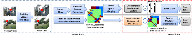
Figure 1: An Overview of our approach: We begin with dividing training videos into multiple non-overlapping clips. Each clip is represented by a single covariance matrix computed from appearance and motion features as explained in Sections  III-A and  III-B. A dictionary is created by stacking up the covariance matrices. Given, a test covariance matrix, its corresponding label is determined by solving a matrix determinant maximization problem as shown in Section III-D. The final label for a video is obtained by aggregating the class labels predicted for individual clips.

These interest point based approaches are incorporated into a traditional bag of video words framework [31] to obtain an intermediate representation of a video that can further be used in a supervised [8] or un-supervised classification [13] algorithm for recognition purposes. While these approaches have been proved to be successful in context of event recognition, since they rely on highly localized statistics over a small spatio-temporal neighborhood [6, 35] e.g. $50\times 50\times 20$ relative to the whole video, different physical motions within this small aperture, are indistinguishable.

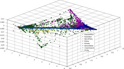
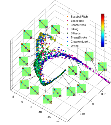
Figure 2: Proposed descriptor vs HOG-HOF [18]: Each circle represents a lower-dimensional manifestation of descriptors from video samples in UCF50 human actions dataset. For legibility, only $8$ classes are shown here using different color codes. 2 HOG-HOF [18] descriptors, originally $162$ dimensional, are reduced to $3$-dimesional for visualization. 2 Proposed descriptor, first vectorized ($190$ dimensional) then mapped to a $3$ dimesional space. Sample covariance matrices are shown as insets to some circular dots. Note how HOG-HOF based descriptors clutter the $3$-D space more as compared to the proposed descriptors, which on the other hand, show relatively clear cluster boundaries. Also, fewer descriptors are shown in Fig. 2 which are clip based, as compared to Fig. 2 which are interest point based. See Fig. 4 for further detailed interpretation.

Also, while describing the statistics of these small neighborhoods, often the temporal and the spatial information are treated independently. For e.g. the HOG-HOF descriptor used in [18] is generated by concatenating two independent histograms : the HOG contributing to the appearance (spatial) and the HOF contributing to motion (temporal). Doing so, the joint statistics between appearance and motion is lost, particularly in case of human action and gesture recognition tasks, where such information can be very useful. For example, consider the example of “pizza-tossing event” from the UCF50  unconstrained actions dataset. Here, a circular white object undergoes a vertical motion which is discriminative for this event class. Precisely, the correlation between white object as captured by appearance features and its associated vertical motion captured basic and kinematic features is well explained in the covariance matrix than a concatenated 1-D histogram of the individual features. It is also important to note that contextual information available in the form of color, gradients etc., is often discriminative for certain action categories. Descriptors that are extensively gradient based such as HOG or HOF, need to be augmented with additional histograms such as color histograms to capture this discriminative information.

In view of the above, we propose a novel descriptor for video event recognition which has the following properties: (1) Our descriptor is a concise representation of a temporal window/clip of subsequent frames from a video rather than localized spatio-temporal patches, for this reason, we do not need any specialized detectors as required by [18, 6, 38], (2) It is based on an effective fusion of motion features such as optical flow and their derivatives, vorticity, divergence etc., and appearance feature such as first and second order derivatives of pixel intensities, which are complementary to each other. This enables the descriptor to be extended to capture other complementary information available in videos e.g. audio, camera motion, very easily, (3) As the descriptor is based on joint distribution of samples from a set of contiguous frames without any spatial subsampling, it is implicitly robust to noise resulting due to slight changes in illumination, orientation etc. (4) It is capable of capturing the correlation between appearance with respect to motion and vice-versa in contrast to concatenated 1-D histograms as proposed in [18, 6, 29, 16], also, since our final descriptor is based on the eigenvectors of the covariance matrix, they automatically transform our random vector of samples into statistically uncorrelated random variables, and (5) Finally being compact, fewer descriptors are required to represent a video compared to local descriptors and they need not be quantized. Fig. 2 provides an insight on the discriminative capability of both the HOG-HOF based descriptors and the proposed covariance matrix based descriptors.

It is the semi-global, compact nature of our descriptor (since it is computed at clip level), that facilitates us to eliminate vector quantization based representation stage which is required in conventional bag-of-visual-words based frameworks, predominantly used in case of local descriptors  [18, 6, 35]. Intuitively, we are interested to explore how contributions of constituent clips can be leveraged to categorize an entire video. In typical sparse representation based classification schemes [39, 23], this issue is well-addressed. This motivates us to explore two sparse representation based techniques to perform event recognition using these covariance matrices as atoms of an over-complete dictionary. In the first one, we map the covariance matrices to an equivalent vector space using concepts from Riemannian manifold before building the dictionary. The classification is performed using a modified implementation of Orthogonal Matching Pursuit [32] which is specifically optimized for sparse-coding of large sets of signals over the same dictionary. We compare this approach with a tensor sparse coding framework [30] formulated as a determinant maximization problem, which intrinsically maps these matrices to an exponential family. Although, our work is largely inspired by [33] and  [30] in object recognition, to the best of our knowledge, ours is the first work that addresses event recognition using a sparse coding framework based on covariance of motion and appearance features.

The rest of this paper is organized as follows: Sect. II discusses some of the related work in this direction. In the next section, we provide the theoretical details of our approach including motion and appearance feature extraction, covariance computation followed by the sparse coding framework for classification. Next, we discuss two interesting applications and provide experimental details on how our descriptor and the classification methods can be applied to address these problems. Finally, Sect. V concludes the paper with future directions.

II Related Work

Covariance matrices as feature descriptors, have been used by computer vision researchers in the past in a wide variety of interesting areas such as: object detection [33, 25, 34, 40], face recognition [24, 30], object tracking [26, 19], etc. The authors of  [33] introduced the idea of capturing low-level appearance based features from an image region into a covariance matrix which they used in a sophisticated template matching scheme to perform object detection. Inspired by the encouraging results, a license plate recognition algorithm is proposed in [25] based on a three-layer, 28-input feed-forward back propagation neural network. The idea of object detection is further refined into human detection in still images [34] and videos [40]. In [34], Tuzel et al. represented the space of d-dimensional nonsingular covariance matrices extracted from training human patches, as connected Riemannian manifold. A priori information about the geometry of manifold is integrated in a Logitboost algorithm to achieve impressive detection results on two challenging pedestrian datasets. This was later extended in [40] to perform detection of humans in videos, incorporating temporal information available from subsequent frames.

The authors of [24] used the idea of using region covariance matrices as descriptors for human faces, where features were computed from responses of Gabor filters of $40$ different configurations. Later, Sivalingam et al. proposed an algorithm [30] based on sparse coding of covariance matrices extracted from human faces, at their original space without performing any exponential mapping as proposed in previous approaches  [33, 25, 34, 40, 24]. In their approach, the authors formulated the sparse decomposition of positive definite matrices as convex optimization problems, which fall under the category of determinant maximization (MAXDET) problems.

In a different vein, Porikli and Tuzel [26] came up with another application of region covariance matrices in context of tracking detected objects in a video. In their technique, the authors capture the spatial and statistical properties as well as their correlation of different features in a compact model (covariance matrix). Finally, a model update scheme is proposed using the Lie group structure of the positive definite matrices which effectively adapts to the undergoing object deformations and appearance changes. Recently, Li and Sun [19] extended the tracking framework proposed in [26], by representing an object as a third order tensor, further generalizing the covariance matrix, which in turn has better capability to capture the intrinsic structure of the image data. This tensor is further flattened and transformed to a reduced dimension on which the covariance matrix is computed. In order to adapt to the appearance changes of the object across time, the authors present an efficient, incremental model update mechanism.

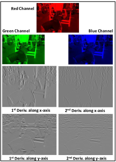
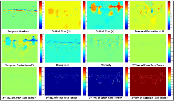
Figure 3: Low-level feature extraction from video clips: 3 Appearance features,and 3 Motion features (basic and kinematic). The kinematic features are derived from optical flow and capture interesting aspect of motion with respect to a spatial neighborhood.

That said, in context of human action and gesture recognition, the exploitation of covariance matrices as feature is relatively inchoate. Some earlier advances are discussed here in this particular direction in order to set the pertinence of this work to the interested reader. Along these lines, the authors of [12] proposed a methodology for detection of fire in videos, using covariance of features extracted from intensities, spatial and temporal information obtained from flame regions. A linear SVM was used to classify between a non-flame and a flame region in a video. Researchers [10, 11] have also attempted to classify simple human actions [28] using descriptors based on covariance matrices. In contrast, our work addresses a more diverse and complex problem. To summarize, we make the following contributions in this work: (1) We propose a novel descriptor for video analysis which captures spatial and temporal variations coherently, (2) Our descriptor is flexible to be used for different application domains (unconstrained action recognition, gesture recognition etc.), and (3) We extensively evaluate two different classification strategies based on concepts from sparse representation that can be used in the recognition pipeline independently.

III Our Approach

In order to make the paper self contained, we briefly describe the theoretical details of all the phases involved in our action recognition computation pipeline, beginning with the feature extraction step. Fig. 1 provides a schematic description of our approach showing the steps involved in training phase (dashed blue box) and the testing phase (dashed red box).

III-A Feature Computation

Since our primary focus is on action recognition in unconstrained scenarios, we attempt to exploit features from both appearance and motion modalities which provide vital cues about the nature of the action. Also since this paper attempts to study how the appearance and motion change with respect to each other, it is important to extract features that are discriminative within a modality. Given a video, we split it into an ensemble of non-overlapping clips of $N$ frames. For every pixel in each frame, we extract the normalized intensities in each channel, first and second order derivatives along the $x$ and $y$ axes. Thus every pixel at $(x,y,t)$ can be expressed in the following vector form with $\mathbf{f_{i}}$, $\mathbf{f_{g}}$ denoting the color and the gray-scale intensity gradient components along the horizontal and vertical axes respectively, as:

$$\mathbf{f_{i}} = \left[R\quad G\quad B\right]^{T},$$

$$\mathbf{f_{g}} = \left[\frac{\partial I}{\partial x}\quad\frac{\partial I}{\partial y}\quad\frac{\partial^{2}I}{\partial x^{2}}\quad\frac{\partial^{2}I}{\partial y^{2}}\right]^{T},$$ (1)

where $R,G,B$ are the red, green, blue intensity channels and $I$ being the gray scale equivalent of a particular frame.

As motion in a video can be characterized using simple temporal gradient (frame difference), horizontal ($u$) and vertical ($v$) components of optical flow vector, we use the following as our basic motion features:

$$\mathbf{f_{m}}=\left[\frac{\partial I}{\partial t}\quad u\quad v\quad\frac{\partial u}{\partial t}\quad\frac{\partial v}{\partial t}\right]^{T},$$ (2)

where $\frac{\partial}{\partial t}$ represents the finite differential operator along the temporal axis. In addition to these basic flow features, we extract high-level motion features [1] derived from concepts of fluid dynamics, since these are observed to provide a holistic notion of pixel-level motion within a certain spatial neighborhood. For e.g. features such as divergence $\nabla$ and vorticity $\Gamma$ quantify the amount of local expansion occurring within flow elements and the tendency of flow elements to “spin”, respectively. Thus

$$\nabla = \frac{\partial u}{\partial x}+\frac{\partial v}{\partial y},$$

$$\Gamma = \frac{\partial v}{\partial x}-\frac{\partial u}{\partial y}.$$ (3)

Local geometric structures present in flow fields can be well captured by tensors of optical flow gradients [1], which is mathematically defined as:

$$G=\begin{pmatrix}\frac{\partial u}{\partial x}&\frac{\partial u}{\partial y}\\ \frac{\partial v}{\partial x}&\frac{\partial v}{\partial y}\end{pmatrix}.$$ (4)

With this intuition, we compute the principal invariants of the gradient tensor of optical flow. These invariants are scalar quantities and they remain unchanged under any transformation of the original co-ordinate system. We determine the second, $\tau_{2}(G)$ and third $\tau_{3}(G)$ invariants of $G$ as:

$$\tau_{2}(G) = \frac{1}{2}\left[tr(G)^{2}+tr(G^{2})\right],$$

$$\tau_{3}(G) = -det(G).$$ (5)

Based on the flow gradient tensor, we determine the rate of strain, $S$ and rate of rotation, $R$ tensors which signify deviations from the rigid body motion, frequently seen in articulated human body movements. These are scalar quantities computed as :

$$S = \frac{1}{2}(G+G^{T}),$$

$$R = \frac{1}{2}(G-G^{T}).$$ (6)

Using the equations in( 5), principle invariants can be computed for these tensors. The interested reader is requested to read [1] for further insights on the selection of invariants. However, unlike the authors of [1], we do not compute the symmetric and asymmetric kinematic features as these assume human motion is centralized which is not valid for actions occurring in an unconstrained manner (typically seen in YouTube videos). For the sake of legibility, we arrange the kinematic features computed from optical flow vectors in the following way,

$$\mathbf{f}_{k}=\left[\nabla\quad\Gamma\quad\tau_{2}(G)\quad\tau_{3}(G)\quad\tau_{2}(S)\quad\tau_{3}(S)\quad\tau_{3}(R)\right]^{T}.$$ (7)

Finally we obtain the following representation for each pixel after concatenating all the above features to form a $19$ element vector as:

$$\mathbf{F}=\left[\mathbf{f_{i}}\quad\mathbf{f_{g}}\quad\mathbf{f_{m}}\quad\mathbf{f}_{k}\right]^{T}.$$ (8)

Figures 3 and 3 visualize the appearance and motion features respectively for a sample frame from the UCF50 dataset, where a person is exercising a “bench-press”.

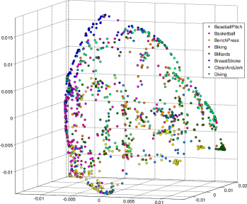
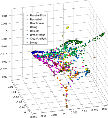
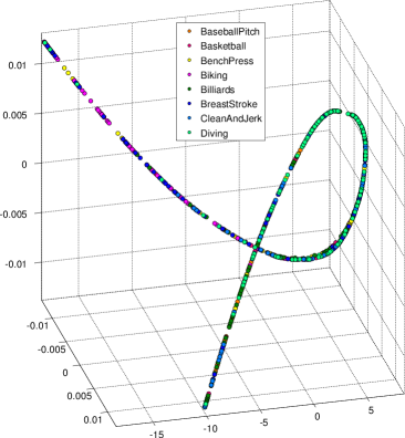
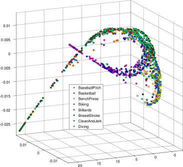
Figure 4: Vector Space Mapping of $S_{n}^{+}$ covariance matrices. The above two figures show covariance matrices (each matrix is a point) from video samples and their respective mapping in log-matrix space. In both the cases, representative video samples from $8$ arbitrary classes in UCF50 are chosen and their respective covariance matrices are determined. Different classes are colored differently. 4 shows original covariance matrices based on appearance features before mapping, and 4 shows the same after mapping. 4 shows original covariance matrices based on motion features before mapping, and 4 shows the same after mapping. Note how some classes show more separability than others after the mapping.

III-B Covariance Computation

Covariance based features introduced by Tuzel and colleagues for object recognition  [33] have found application in various other related areas such as: face recognition [24, 30], shape modeling [36], and object tracking [26]. Based on an integral image formulation as proposed in [33], we can efficiently compute the covariance matrix for a video clip where each pixel is a sample. The covariance matrix in this context is therefore computed as :

$$C=\frac{1}{n-1}\sum_{i=1}^{n}(\mathbf{f^{(k)}_{i}}-\mu)(\mathbf{f^{(k)}_{i}}-\mu)^{T},$$ (9)

where $\mathbf{f^{(k)}}$ is a single feature set and $\mu$ is its corresponding mean, $n$ being the number of samples (here pixels). Since the covariance matrix is symmetric, it contains $(d^{2}+d)/2$ ($d$ being the total types of features) unique entries forming the upper or lower triangular part of the matrix, that capture cross feature set variance.

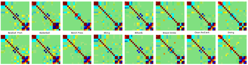
Figure 5: Normalized Covariance matrices from $8$ class of actions from UCF50: Each column shows a different class, and each row is a sample covariance matrix constructed from clips belonging to one of the $8$ classes. We can notice the subtle differences between two samples of different classes and some structural similarity of elements of the same class. This aspect is more pronounced in Fig. 2.

Covariance matrices have some interesting properties which naturally suits our problem. Since these matrices do not have any notion of the temporal order in which samples are collected, they are computationally more favorable compared to trajectory based descriptors [35] that require explicit feature tracking. Secondly, covariance based descriptors provide a better way of analyzing relationship across feature sets compared to mere concatenation of histograms of different features [18]. Furthermore, the covariance matrices provide more concise representation of the underlying feature distribution due to symmetry compared to long descriptors generated by methods proposed in [29, 6] which need additional dimensionality reduction. We visualize descriptors computed from covariance matrices in figures 4,  5.

Since, the covariance matrices are symmetric, either the upper or lower triangular elements can be used to form a vector $\in\mathbb{R}^{l},l=(d^{2}+d)/2$ describing a clip. However, with that being said, vector addition and scalar multiplication $\in\mathbb{R}^{l}$, is not closed [9], as the matrices conform to non-linear connected Riemannian manifolds of positive definite matrices ($S_{n}^{+}$). Hence, the descriptors obtained by direct vectorization as explained above, cannot be used as they are, for classification using regular machine learning approaches ($\mathbb{R}^{2}$). One possible approach to address this issue is to map these matrices to an equivalent vector space closed under addition or scalar multiplication, in order to facilitate classification tasks.

Fortunately, such an equivalent vector space for positive definite matrices exists, where these matrices can be mapped to the tangent space of the Riemannian manifolds [2]. There are a couple of advantages of using this transformation, besides of the utility of being used in linear classification algorithms. The distance metric defined in this transformed subspace, is affine invariant and satisfies triangle inequality  [9]. Such transformation of a covariance matrix $C$ to its log $L$ can be performed using:

$$L=\log(C)=R^{T}\hat{D}R,$$ (10)

where $R^{T},R$ are rotation matrices obtained after singular value decomposition of $C$ and $\hat{D}$ is the diagonal matrix containing the log of eigenvalues. The mapping results in a symmetric matrix whose upper or lower triangular components form our final feature descriptor for a given video clip.

Although these descriptors can be directly used in any vector quantization based bag-of-visual-words representation for classification tasks as used in  [18, 35], there is a major disadvantage. The matrix logarithm operation in Eqn. (10), due to its tangent space approximation of the original symmetric positive semi-definite space of covariance matrices, decimates structural information inherent to the matrices. Thus, further quantization performed in typical bag-of-visual-words based frameworks, can be detrimental towards the overall classification accuracy. We validate this empirically later in Sect. IV-A2. Therefore, we propose the use of sparse representation based techniques for our classification problem, which eliminates further quantization of these descriptors, thereby leveraging on the existing available information.

III-C Sparse coding of Matrix Log Descriptors

Recently, sparse linear representation techniques have shown promising results in solving key computer vision problems including face recognition [39], object classification [23] and action recognition [10]. The basic objective of these approaches is to project the classification problem into a sparse linear approximation problem. Formally, given a set of $K$ training samples consisting of $k$ classes, $\mathbf{A}_{1},\mathbf{A}_{2},\ldots,\mathbf{A}_{K}$ and a test sample $\mathbf{y}$, an over-complete dictionary $A$ is constructed by stacking the training samples. Then the approximation problem:

$$\min||\mathbf{x}||_{1}\quad s.t.\quad\mathbf{y}=A\mathbf{x}$$ (11)

where $\mathbf{x}$ is a sparse vector of coefficients corresponding to each element in $A$, can be solved using linear programming techniques. For each coefficient in $\mathbf{x}$, the residuals :

$$r_{i}=||\mathbf{y}-A\mathbf{x}_{i}||_{2}$$ (12)

are computed, where $\mathbf{x_{i}}$ is a zero vector with $i$th entry set to the $i$th coefficient in $\mathbf{x}$. The smallest residual identifies the true label of $\mathbf{y}$.

Since, we have multiple descriptors per training sample, we modify the above formulation to suit our problem in the following way: Given a set of $p$ clips from training videos, we construct our over-complete dictionary ($A$ in (11)) by stacking corresponding matrix log descriptors which are obtained after applying Eqn. (10). Thus, for a query video containing $m$ descriptors $\mathbf{y_{1}}\ldots\mathbf{y_{m}}$ from as many clips, our objective is to find how each of these clips can be efficiently approximated jointly using a linear combination of a subset of elements from $A$. Mathematically the problem can be stated as:

$$\mathbf{L}=\left.\begin{array}[]{lll}\min||\mathbf{y}_{1}&-&A\mathbf{x}||_{2}^{2},\\ &\vdots&\\ \min||\mathbf{y}_{m}&-&A\mathbf{x}||_{2}^{2},\end{array}\right\}\text{s.t.}||\mathbf{x}||_{0}\leq P,$$ (13)

with $||\mathbf{x}||_{0}$ the $l_{0}$ pseudo-norm equal to the number of nonzero coefficients in $\mathbf{x}$, $P$ being an empirically determined threshold to control the degree of sparsity. Eqn. (13) can be solved efficiently using batch version of the orthogonal matching pursuit [32] , which computes the residuals jointly $\forall\mathbf{y}_{j}$, by constraining the coefficients in $\mathbf{x}$ to be orthogonal projections of all clips in query sample $y$ on the dictionary $A$. Since each element in $A$ is associated with a label indicating the class from which the clip is extracted, the solution to Eqn. (13) yields $\mathbf{L}\in\mathbb{R}^{m}$, containing labels corresponding to each clip from the query video. The final label of the video can be obtained using a simple majority voting of the labels in $\mathbf{L}$.

The technique discussed above can be viewed as a straight-forward solution to our problem. However, the above framework is only applicable to vector spaces. Thus, although it retains more information as compared to vector quantization based methods in this context, it is unable to exploit the information available in the structure of the covariance matrices which conform to Riemannian geometry. This motivates us to explore further on the recent advances of Sivalingam and colleagues [30] in sparse coding of covariance matrices which is discussed as follows.

III-D Tensor Sparse Coding of Covariance Matrices

Consider our query video consists of a single clip whose motion-appearance covariance matrix $Q$, constructed using Eqn. 9, can be expressed as a linear combination of covariance matrices forming an over-complete dictionary $D$:

$$Q=x_{1}D_{1}+x_{2}D_{2}+\ldots+x_{p}D_{p}=\sum_{i=1}^{p}x_{i}D_{i},$$ (14)

where $x_{i}$’s are coefficients of the elements $D_{i}$ from dictionary $D$ of covariance matrices of labeled training videos. As $Q$ belongs to the connected Riemannian manifold of symmetric positive definite matrices, the following constraint is implied:

$$\hat{Q}\succeq 0,\Rightarrow x_{1}D_{1}+x_{2}D_{2}+\ldots+x_{p}D_{p}\succeq 0,$$ (15)

where $\hat{Q}$ is the closest approximation of $Q$, introduced to handle noise in real-world data. This closest approximation can be achieved by solving an optimization problem. However, in order to perform this task, we first need to define a measure of proximity between our query matrix $Q$ and the approximated solution $\hat{Q}$. Such a proximity measure is often measured in terms of penalty function called LogDET or Burg matrix Divergence [14] which is defined as:

$$\Phi_{\nabla}(\hat{Q},Q)=tr(\hat{Q}Q^{-1})-\log\det(\hat{Q}Q^{-1})-d,$$ (16)

Using Eqn.(14), the above equation can be further expanded as:

$$\Phi_{\nabla}(Q,\hat{Q})=tr(\sum_{i=1}^{p}x_{i}D_{i}{Q}^{-1})-\log\det(\sum_{i=1}^{p}x_{i}D_{i}{Q}^{-1})-d,$$ (17)

Since, $\hat{D_{i}}=Q^{-1/2}D_{i}Q^{-1/2}$, we can substitute Eqn.(17) appropriately, achieving:

$$\Phi_{\nabla}(Q,\hat{Q}) = tr(\sum_{i=1}^{p}x_{i}\hat{D}_{i})-\log\det(\sum_{i=1}^{p}x_{i}\hat{D}_{i})-d,$$

$$= \sum_{i=1}^{p}x_{i}tr(\hat{D}_{i})-\log\det(\sum_{i=1}^{p}x_{i}\hat{D}_{i})-d,$$

where the $\log\det(.)$ function can be expressed as Burg Entropy of eigenvalues of a matrix $Z$ as $\log\det(Z)=\sum_{i}\log{\lambda_{i}}$. Therefore, our optimization problem can be formulated using the objective function in Eqn.( LABEL:eqn:final) as:

$$\min_{x} \sum_{i=1}^{p}x_{i}tr(\hat{D}_{i})-\log\det(\sum_{i=1}^{p}x_{i}\hat{D}_{i})+\delta||\mathbf{x}||_{1}$$

subject to $$\mathbf{x}\geq 0,\quad\sum_{i=1}^{p}x_{i}\hat{D_{i}}\succeq 0,\text{and},\quad\sum_{i=1}^{p}x_{i}\hat{D_{i}}\preceq I_{n}$$

with, $\delta||\mathbf{x}||_{1}$ being a relaxation term that incorporates sparsity. The above problem can be mapped to a determinant maximization problem which can be efficiently solved by semi-definite programming techniques. The optimization in Eqn.  (LABEL:eqn:maxdet) can be performed separately for all $m$ clips in a video and the labels can be combined in the similar way as discussed in case of matrix log descriptors, leading to final label for a query sample. In the next sections, we provide our experimental details comparing the approaches presented here on two different application domains, finally discussing the results at the end of each sections.

IV Experiments

We organize this section into two parts that address two different problems in video analysis encountered in practical scenarios. In the first one, we emphasize on action recognition in unconstrained case. The next part elucidates our observations on another important problem : one-shot recognition of human gestures.

IV-A Human Action Recognition

This is an extremely challenging problem, especially because videos depicting actions are captured in diverse settings. There are two newly introduced, challenging datasets (UCF50, HMDB51 [17]) containing videos that reflect such settings (multiple and natural subjects, background clutter, jittery camera motion, varying luminance). To systematically study the behavior of our proposed descriptor and the associated classification methods, we conduct preliminary experiments on a relatively simple, well recognized, human actions dataset [28] to validate our hypothesis and then proceed towards the unconstrained case.

IV-A1 Datasets

KTH Human Actions: This dataset [28] consists of $6$ classes namely: Boxing, Clapping, Jogging, Running, Walking, and Waving. The dataset is carefully constructed in a restricted environment – clutter-free background, exaggerated articulation of body parts not seen in real-life, mostly stable camera except for controlled zooming with single human actors. The videos in this dataset are in gray scale and not much cue is useful from background.

UCF50: The UCF50, human actions dataset consists of video clips that are sourced from YouTube videos (unedited) respectively. It consists of over $6,500$ RGB video clips (unlike KTH) distributed over $50$ complex human actions such as horse-riding, trampoline jumping. baseball pitching, rowing etc. This dataset has some salient characteristics which makes recognition extremely challenging as they depict random camera motion, poor lighting conditions, huge foreground and background clutter, in addition to frequent variations in scale, appearance, and view points. To add to the above challenges, since most videos are shot by amateurs with poor cinematographic knowledge, often it is observed that the focus of attention deviates from the foreground.

HMDB51: The Human Motion DataBase [17], introduced in 2011, has approximately $7,000$ clips distributed over $51$ human motion classes such as : brush hair, push ups, somersault etc. The videos have approximately $640\times 480$ spatial resolution, and are mostly sourced from TV shows and movies. The videos in the dataset are characterized by significant background clutter, camera jitter and to some extent the other challenges observed in the UCF50 dataset.

IV-A2 Experimental Setup

We make some adjustments to the original covariance descriptor by eliminating appearance based features in Eqn.(8) to perform evaluations on the KTH dataset, as not much contextual information is available in this case. Thus each pixel is represented by a $12$ dimensional feature vector (last $12$ features from $\mathbf{F}$ in 8) resulting in a $(12^{2}+12)/2=78$ dimensional vector. Each video is divided into uniformly sampled non-overlapping clips of size $w\times h\times t$, $w,h$ being the original resolution of the video and $t$ is the temporal window. Throughout all experiments, we maintain $t=20$. Optical flow which forms the basis of our motion features, is computed using an efficient GPU implementation[4].

For all classification experiments we use a split-type cross-validation strategy suggested by the authors in [28]. We ensure that the actors that appear in the validation set do not appear in the training set to construct a dictionary for fair evaluation. Similar split strategy is employed for experiments on UCF50. For HMDB51 we follow the authors validation strategy that has three independent splits. The average performance across all splits is recorded in Tables II and I.

In order to make fair comparison of our novel covariance based descriptor to a popular interest point based feature representation [18], we use a traditional bag-of-visual-words framework for the latter. This forms our first baseline for all datasets (indicated as first row in Tab.  I). Next, we compare the proposed sparse representation based classification framework against three independent strategies, using slightly different versions of our covariance descriptor. In the first, the covariance matrices are naively vectorized and the upper-triangular elements are used as clip-level descriptors. In the second, they are vectorized using the Eqn. (10) discussed in Sect. III-B. Each clip is used to train multi-class linear SVMs [8] and for a query, labels corresponding to each clip are aggregated in a majority voting scheme (Sect.  III-C). In the next setting, we use a bag-of-visual-words framework for representing a video where the vocabulary is constructed by vector quantization of matrix log descriptors of covariance matrices. Experiments with different codebook sizes $64,128,256,512,1024,2048$ are conducted. Although the selection of codebook size is dataset specific, we observed recognition accuracies becoming asymptotic after relatively less codebook sizes ($128$ for KTH, $512$ for both UCF50 and HMDB51). A histogram intersection kernel based SVM is used as a final classifier.

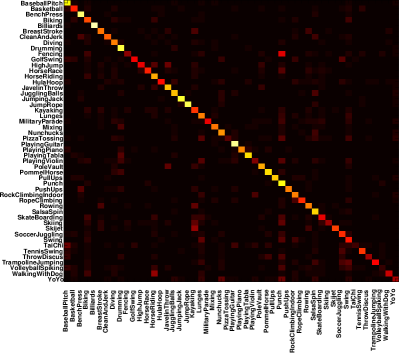
Figure 6: Confusion matrix obtained after performing classification using the proposed classification technique on the UCF50.

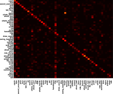
Figure 7: Confusion matrix obtained after performing classification using the proposed classification technique on HMDB51 dataset.

IV-A3 Results

In Tab. I, we present a comparative analysis of the various classification methods on these datasets. We compare our methods with the state of the art performance obtained by other competitive approaches. Although our proposed method does not show significant improvement over the state of the art on the KTH dataset, we observe definite increase in performance over the two other challenging action recognition datasets. We also observe that there is a steady increase in performance across all datasets as we change our classification strategies that are more adapted to the matrix based descriptors which intuitively argues in favor of our original hypothesis. The reason can be attributed to vector quantization of the matrix based descriptors in the bag-of-visual-words representation (row $2-3$ of Tab.  I). Proper vectorization using the matrix log mapping (Eqn. 10) increases the accuracy by $3-6\%$ (row $4$), which is further improved when sparse representation based classification is employed (row $5$). Finally, tensor sparse coding of covariance matrices (row $6$), achieves the best performance across all datasets. Note that the performance reflected in case of UCF50 and HMDB51 datasets are significantly high as compared to other approaches as a lot of contextual information is available from the RGB channels of the video.

		Datasets
Method	Desc.	KTH	UCF50	HMDB51
BoVW	HOG-HOF [18]	92.0%	48.0%	20.2%
BoVW	COV	81.3%	39.3%	18.4%
SVM	COV	82.4%	40.4%	18.6%
SVM	LCOV	86.2%	47.4%	21.03%
OMP	LCOV	88.2%	53.5%	24.09%
TSC	MAT	93.4%	57.8%	27.16%

TABLE I: Comparison with the state-of-the-art methods: This table summarizes the performance of two of our proposed methods with different feature representations and classification strategies. First row shows the avg. recognition accuracies on a typical bag-of-visual-words framework on top of interest point based HOG-HOF descriptors [18]. In the next row, naively vectorized versions of the covariance matrices (COV) are used as descriptors in a similar BoVW framework. The next two rows reflect the same obtained after keeping linear SVM as classifiers using naive vectorization and matrix log descriptors (LCOV) as features. Finally the contributions of the proposed sparse representation based classification schemes – Orthogonal Matching Pursuit (OMP) on LCOV and Tensor Sparse Coding (TSC) on the original covariance matrices (MAT) is highlighted in the two bottom rows, respectively.

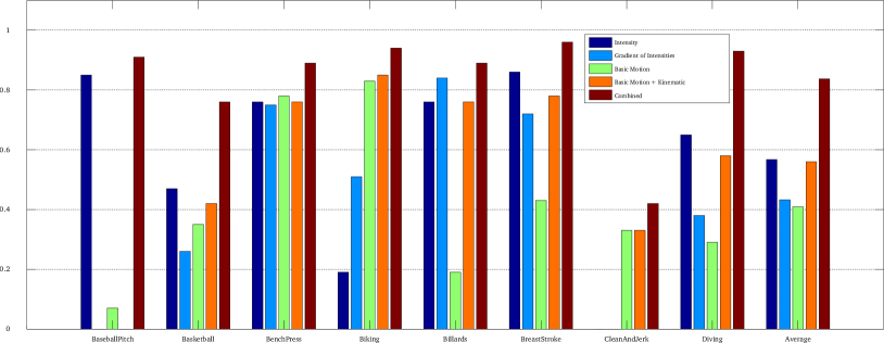
Figure 8: F-measures for $8$ classes from UCF50 dataset with different features. The features experimented with are as follows : $\mathbf{F_{i}}$ (RGB Intensities), $\mathbf{F_{g}}$ (Intensity gradients), $\mathbf{F_{m}}$ (Basic Motion Features i.e. temporal derivatives, optical flow etc.), $\mathbf{F_{k}}$ (Kinematic Features), A combination of basic motion and kinematic features and finally all features are used together in the covariance descriptor.

Given matrix log descriptors as feature, among linear SVM and OMP based classification, we observe OMP perform better than the former which shows that there is an inherent sparsity in the data which is favored by sparse representation based classification techniques. In Fig. 6 and Fig. 7, we present the confusion matrices obtained after classification using the tensor sparse coding which performs the best in case of both the datasets. In UCF50, the highest accuracies are obtained for classes that have discriminative motion (e.g. Trampoline jumping is characterized by vertical motion as opposed to other action categories). In case of action classes Skijet, Kayaking and Rowing, we observe high degrees confusion, as in all cases the low-level appearance components (water) in the covariance descriptors dominate over the motion components. A similar behavior is observed in case of two action classes in particular – Punch and Drumming which show confusion with at least $5$ other classes which also occur mostly in indoor scenarios. In order to provide a profound insight, we analyze the individual low-level feature set contributions towards the recognition accuracies.

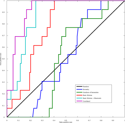
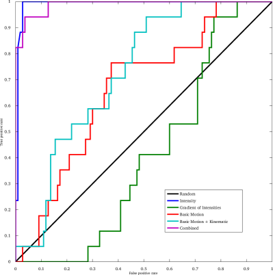
Figure 9: Precision-Recall curves for detection of 9 CleanAndJerk and 9 BaseballPitch samples from UCF50. Of the $8$ classes analyzed in Fig. 8, these are the two classes which have clear separation because of their distinctive motion features.

Low-level Feature Set Contributions: To investigate the contribution of different feature modalities towards the recognition performance, we computed $3$ different sets of covariance matrices for videos in UCF50. Firstly, descriptors computed using only appearance features (resulting in a $7\times 7$ matrix). Next, we use only motion based features. Thus the covariance matrix in this case is $12\times 12$. Finally, both appearance and motion features are used together to compute the covariance matrices. We also evaluated how each classification strategy behaves with these different descriptors. For each of these descriptors, the classification framework was varied between a linear SVM (SVM/LCOV), Sparse OMP (OMP/LCOV), and finally the Tensor Sparse Coding (TSC) algorithm that uses MAXDET optimization. For the first two methods, the descriptors are of the following dimensions: $28$ (appearance), $78$ (motion) and $190$ (all).

We observed that the appearance features are less informative as compared to the motion features in videos where RGB information is available. However, all classification techniques get a boost in performance when both the features are used together, which shows how the proposed descriptor captures complementary information. Tensor Sparse Coding based classification performs better than other two methods. Tab. II summarizes the results of the experiments involving the contribution of different feature modalities and methods. The different columns in the table show the feature modalities used for computing the covariance matrices (AF = Appearance Features, MF = Motion Features, AMF = Appearance and Motion Features).

The individual feature contribution towards the overall classification performance, is further experimented with finer granularity. Fig. 8 indicates F-measures derived from precision and recall for $8$ different classes of unconstrained actions from UCF50 dataset. It is interesting to notice two distinct trends from this experiment: RGB intensities contribute the most towards the discriminativity of the covariance descriptor for Baseballpitch while CleanAndJerk is best described by motion features. This can be explained by the sudden vertical motion captured by the basic motion and kinematic features in CleanAndJerk samples, and the mostly greener texture of background captured by intensity features in Baseball-pitch samples. The Precision-Recall curves for detection of these classes are provided in Fig. 9, emphasize the contribution of the features in further finer granularity. The following section provides a brief discussion on the algorithmic complexities involved in the various steps of the entire recognition pipeline.

		Experiments on UCF50
Method	Desc.	AF	MF	AMF
SVM	LCOV	31.4%	43.4%	47.4%
LC/OMP	LCOV	34.2%	42.5%	51.5%
TSC	MAT	34.5%	46.8%	53.8%

TABLE II: Contribution of feature sets and methods on UCF50: First row shows Matrix Log descriptors (LCOV) from covariances with linear SVM classifier, second row - LCOV with sparse OMP classifier, and finally Tensor Sparse Coding (TSC) on Covariance Matrices (MAT). Columns show the feature modalities used for computing the covariance matrices (AF = Appearance Features, MF = Motion Features, AMF = Appearance and Motion Features combined).

IV-A4 Complexity Analysis

The entire computation pipeline can be summarized in three major steps, namely low-level feature extraction, feature fusion using covariance matrices, followed by classification. Off these, the feature extraction and covariance computation step for each clip of a video can be done in parallel for any dataset. Among feature extraction, optical flow computation [4] is the most expensive step, which is based on a variational model. For a consecutive pair of frames, with a resolution of $512\times 384$, a GPU implementation of the above algorithm, takes approximately $5$ seconds on a standard desktop computer hosting a 2.2Ghz CPU with 4GB of physical memory. Depending on the types of low-level features computed, the complexity of the covariance matrix computation is $O(WHdC)$ where $d$ is the total types of low-level features, $W$ and $H$ are the respective width and height of a typical clip, and $C$ being the total number of frames per clip.

The complexity of classification using the Orthogonal Matching Pursuit[32] scheme is optimized using an efficient batch implementation provided in[27]. Since this method involves precomputation of an in-memory dictionary of fixed number of elements ($T_{D}$), the overall complexity can be approximated as $O(T_{D}+K^{2}d+3Kd+K^{3})$, where $K$ is the target sparsity for sparse coding. For details, please refer [27]. Classification using MAXDET optimization, on the other hand, is relatively more expensive as it attempts to find a subset of dictionary atoms representing a query sample using a convex optimization. In closed form, this is $O(d^{2}L^{2})$, $L$ being the number of dictionary atoms. Although, this technique is more reliable in terms of accuracy, it requires a larger computation overhead as the process needs to be repeated for every query sample. Assuming the number of samples are far larger than $L$ batch-OMP is observed to offer a respectable trade-off between accuracy and speed.

IV-B One-shot Learning of Human Gestures

In addition, to demonstrate the applicability of our video descriptor, we report our preliminary experimental results on different application domain: human gesture recognition using a single training example.

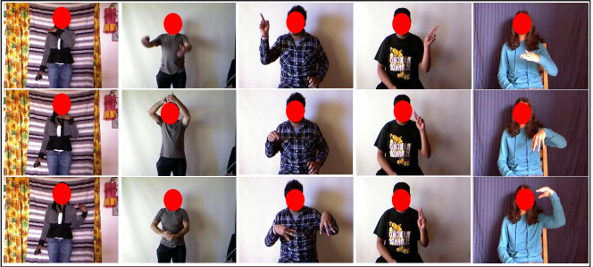
Figure 10: Sample frames from representative batches from the CGD 2011 dataset.

IV-B1 ChaLearn Gesture Data (CGD) 2011

This dataset is compiled from human gestures sampled from different lexicons e.g. body language gestures (scratching head, crossing arms etc.), gesticulations performed to accompany speech, sign languages for deaf, signals (referee signals, diving signals, or marshaling signals to guide machinery or vehicle) and so on. Within each lexicon category, there are approximately, $50$ video samples organized in different batches, captured using depth and RGB sensors provided by the Kinect  platform. Each video is recorded at $30$ Hz at a spatial resolution of $640\times 480$. Each batch is further divided into training and testing splits and only a single example is provided per gesture class in the training set. The objective is to predict the labels for the testing splits for a given batch.

Although the videos are recorded using a fixed camera under homogeneous lighting and background conditions, with a single person performing all gestures within a batch, there are some interesting challenges in this dataset. These are listed as follows: (1) Only one labeled example of each unique gestures, (2) Some gestures include subtle movement of body parts (numeric gestures), (3) Some part of the body may be occluded, and, (4) Same class of gesture can have varying temporal length across training and testing splits.

	Descriptor Performance(%)
Batch ID	M	MG	MP	All
Devel01	66.7	66.7	88.3	83.3
Devel02	53.3	66.7	53.3	75.0
Devel03	28.6	42.9	21.4	28.6
Devel04	53.3	58.3	75.0	75.0
Devel05	92.8	100	92.8	100.0
Devel06	83.3	91.7	83.3	91.7
Devel07	61.5	76.9	61.5	84.6
Devel08	72.7	72.7	81.8	81.8
Devel09	69.2	61.5	69.2	69.2
Devel10	38.5	61.5	53.6	53.6
Avg.	62.9	69.9	68.0	74.3

TABLE III: Contribution of different low level features towards the one-shot gesture learning problem: Each column shows a different set of low-level features used to compute the final descriptor. The order of low-level feature sets are as follows: Basic Motion (M), Basic Motion and Intensity gradients (MG), Subset of Basic motion and positional informations (MP), and finally all features combined. Refer to Section IV-B2 for more details.

IV-B2 Experimental Setup

We obtain a subset of $10$ batches from the entire development set to perform our experiments. For a given batch, the position of the person performing the gesture remains constant, so we adjust our feature vector in Eqn.(8) to incorporate the positional information of the pixels $x,y,t$ in the final descriptor. Furthermore, since the intensities of the pixels remain constant throughout a given batch, the RGB values at the corresponding pixel locations could also be eliminated. Also, the higher order kinematic features such as $\tau_{2}(S)$, $\tau_{3}(S)$, and $\tau_{3}(R)$ can be removed as they do not provide any meaningful information in this context. Thus each pixel is represented in terms of a $16$ dimensional feature vector, resulting in a $16\times 16$ covariance matrix with only $136$ unique entries. The upper triangular part of the log of this matrix forms our feature descriptor for a clip extracted from a video. In order to perform classification, we use a nearest neighbor based classifier with the same clip-level voting strategy as discussed in the earlier experiments. A regular SVM based classifier is not applicable to this problem as there is only one training example from each gesture class.

Since depth information is available along with the RGB videos, we exploit it to remove noisy optical flow patterns generated by pixels in the background, mainly due to shadows.

	Method Acc. Avg. (%)
Batch ID	MBH/NN	STIP/NN	TPM	LCOV/NN
Devel01	66.7	25.0	58.3	83.3
Devel02	33.4	8.3	25.0	75.0
Devel03	7.2	28.6	14.3	28.6
Devel04	33.4	16.7	58.4	75.0
Devel05	28.6	14.3	64.3	100.0
Devel06	50.0	16.7	25.0	91.7
Devel07	23.1	7.7	15.4	84.6
Devel08	36.4	9.09	9.1	81.8
Devel09	30.7	23.1	53.8	69.2
Devel10	15.4	15.4	23.1	53.6
Avg.	32.4	16.4	34.7	74.3

TABLE IV: Comparison with other features/methods: This table summarizes the performance of our descriptor in one-shot gesture recognition against other methods. The leftmost column contains the batches on which the methods are tested. The next two columns contain indicate the avg. accuracy obtained using two local feature based approaches: MBH  [35] and STIP [18] using a Nearest Neighbor (NN) classifier, the next column uses template matching (TPM) based method and the last column records the performance of our descriptor (LCOV) when used with a nearest neighbor classifier.

IV-B3 Results

Similar to the previous experiments on action recognition in section  IV-A, we perform a detailed analysis, with more emphasis on the descriptor. To this end, we use different versions of the descriptor with only motion features (M:$9\times 9$ covariance matrix), a combination of motion and intensity gradients (MG:$13\times 13$ covariance matrix), a combination of motion and positional information (MP:$12\times 12$ covariance matrix) and finally all features combined ($16\times 16$). The results are reported in Tab.  III. We observe that again motion in itself is not the strongest cue. However, when fused with appearance gradients and positional information, the overall performance of the descriptor increases by $11\%$, which is a significant improvement considering the nature of the problem.

In order to make a fair evaluation of our descriptor with the state-of-the-art descriptors from action recognition literature [18, 35], we keep the classifier constant (Nearest Neighbor). We also compared our approach with a simple template matching based recognition which is more appropriate for this type of problem. The average accuracies for each batch tested using all the compared methods are reported in Table IV. It is pleasing to note that our descriptor performs significantly better than all other methods which gives us promising leads towards the applicability of this descriptor for this class of problems. Finally, in Fig. 11, we show the respective confusion matrices obtained after applying the proposed method on first $10$ of the development batches from the CGD 2011 dataset.

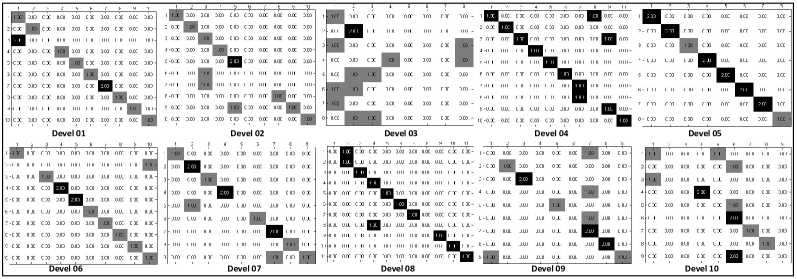
Figure 11: Confusion matrices obtained after applying the proposed method on first $10$ of the development batches from the CGD 2011 dataset. Note for certain batches (devel01–02, devel04–05, devel06–08), our method is able to predict gesture labels with respectable accuracies using just one training sample.

V Conclusion & Future Work

We presented an end-to-end framework for event recognition in unconstrained scenarios. As part of this effort, we introduced a novel descriptor for general purpose video analysis that is an intermediate representation between local interest point based feature descriptors and global descriptors. We showed that how simple second order statistics from features integrated to form a covariance matrix can be used to perform video analysis. We also proposed two sparse representation based classification approaches that can be applied to our descriptor. As part of future work, we intend to fuse more information in our proposed descriptor such as audio and would like to explore on optimizing the MAXDET approximation problem which is currently a computationally expensive operation in our recognition framework.

References

- [1] S. Ali and M. Shah. Human action recognition in videos using kinematic features and multiple instance learning. IEEE Trans. Pattern Anal. Mach. Intell., 32(2):288–303, 2010.
- [2] V. Arsigny, P. Fillard, X. Pennec, and N. Ayache. Log-euclidean metrics for fast and simple calculus on diffusion tensors. Magnetic Resonance in Medicine, 56(2):411–421, aug 2006.
- [3] H. Bay, T. Tuytelaars, and L. V. Gool. Surf: Speeded up robust features. In In ECCV, pages 404–417, 2006.
- [4] A. Chambolle and T. Pock. A first-order primal-dual algorithm for convex problems with applications to imaging. Journal of Mathematical Imaging and Vision, 40(1):120–145, 2011.
- [5] N. Dalal and B. Triggs. Histograms of oriented gradients for human detection. In In CVPR, pages 886–893, 2005.
- [6] P. Dollar, V. Rabaud, G. Cottrell, and S. Belongie. Behavior recognition via sparse spatio-temporal features. 2005. IEEE International Workshop on VS-PETS.
- [7] L. Duan, D. Xu, I. W.-H. Tsang, and J. Luo. Visual event recognition in videos by learning from web data. IEEE Transactions on Pattern Analysis and Machine Intelligence, 99, 2011.
- [8] R.-E. Fan, P.-H. Chen, and C.-J. Lin. Working set selection using second order information for training support vector machines. J. Mach. Learn. Res., 6:1889–1918, 2005.
- [9] W. Forstner and B. Moonen. A metric for covariance matrices, 1999.
- [10] K. Guo, P. Ishwar, and J. Konrad. Action recognition in video by sparse representation on covariance manifolds of silhouette tunnels. In Proceedings of the 20th International conference on Recognizing patterns in signals, speech, images, and videos, ICPR’10, pages 294–305, 2010.
- [11] K. Guo, P. Ishwar, and J. Konrad. Action recognition using sparse representation on covariance manifolds of optical flow. In Advanced Video and Signal Based Surveillance (AVSS), 2010 Seventh IEEE International Conference on, pages 188–195, 2010.
- [12] Y. Habiboglu, O. Gunay, and A. Çetin. Covariance matrix-based fire and flame detection method in video. Machine Vision and Applications, pages 1–11, September 2011.
- [13] T. Hastie and R. Tibshirani. Discriminant adaptive nearest neighbor classification. IEEE Trans. Pattern Anal. Mach. Intell., 18:607–616, June 1996.
- [14] W. James and J. Stein. Estimation with Quadratic Loss. In Proceedings of the Third Berkeley Symposium on Mathematical Statistics and Probability, pages 361–379, 1961.
- [15] Y.-G. Jiang, X. Zeng, G. Ye, S. Bhattacharya, D. Ellis, M. Shah, and S.-F. Chang. Columbia-UCF TRECVID2010 multimedia event detection: Combining multiple modalities, contextual concepts, and temporal matching. In NIST TRECVID Workshop, 2010.
- [16] A. Kläser, M. Marszałek, and C. Schmid. A spatio-temporal descriptor based on 3d-gradients. In British Machine Vision Conference, pages 995–1004, 2008.
- [17] H. Kuehne, H. Jhuang, E. Garrote, T. Poggio, and T. Serre. HMDB: a large video database for human motion recognition. In ICCV, 2011.
- [18] I. Laptev and T. Lindeberg. Space-time interest points. In IN ICCV, pages 432–439, 2003.
- [19] P. Li and Q. Sun. Tensor-based covariance matrices for object tracking. In ICCV Workshops, pages 1681–1688, 2011.
- [20] J. Liu, J. Luo, and M. Shah. Recognizing realistic actions from videos “in the wild”. In IEEE Conference on Computer Vision and Pattern Recognition, 2009.
- [21] J. Liu and M. Shah. Scene modeling using co-clustering. In Computer Vision, 2007. ICCV 2007. IEEE 11th International Conference on, pages 1–7, 2007.
- [22] D. G. Lowe. Distinctive image features from scale-invariant keypoints. IJCV, 60(2), 2004.
- [23] J. Mairal, F. Bach, J. Ponce, G. Sapiro, and A. Zisserman. Discriminative learned dictionaries for local image analysis. In Computer Vision and Pattern Recognition, 2008. CVPR 2008. IEEE Conference on, pages 1 –8, june 2008.
- [24] Y. Pang, Y. Yuan, and X. Li. Gabor-based region covariance matrices for face recognition. IEEE Trans. Circuits Syst. Video Techn., 18(7), 2008.
- [25] F. Porikli and T. Kocak. Robust license plate detection using covariance descriptor in a neural network framework. In Proceedings of the IEEE International Conference on Video and Signal Based Surveillance, AVSS ’06, pages 107–, 2006.
- [26] F. Porikli, O. Tuzel, and P. Meer. Covariance tracking using model update based on lie algebra. In CVPR (1), 2006.
- [27] R. Rubinstein, M. Zibulevsky, and M. Elad. Efficient implementation of the k-svd algorithm using batch orthogonal matching pursuit. Technical report, Computer Science Department, Technion (Israel Institute of Technology), 2008.
- [28] C. Schuldt, I. Laptev, and B. Caputo. Recognizing human actions: A local SVM approach. In ICPR, 2004.
- [29] P. Scovanner, S. Ali, and M. Shah. A 3-dimensional sift descriptor and its application to action recognition. In Proceedings of ACM MM, 2007.
- [30] R. Sivalingam, D. Boley, V. Morellas, and N. Papanikolopoulos. Tensor sparse coding for region covariances. In Proceedings of the 11th European conference on Computer vision: Part IV, pages 722–735, 2010.
- [31] X. Sun, M. Chen, and A. Hauptmann. Action recognition via local descriptors and holistic features. In Computer Vision and Pattern Recognition Workshop, 2009.
- [32] J. Tropp and A. Gilbert. Signal recovery from random measurements via orthogonal matching pursuit. Information Theory, IEEE Transactions on, 53(12):4655 –4666, dec. 2007.
- [33] O. Tuzel, F. Porikli, and P. Meer. Region covariance: A fast descriptor for detection and classification. In ECCV (2), pages 589–600, 2006.
- [34] O. Tuzel, F. Porikli, and P. Meer. Human detection via classification on riemannian manifolds. In IEEE CVPR, pages 1–8, 2007.
- [35] H. Wang, A. Kläser, C. Schmid, and L. Cheng-Lin. Action recognition by dense trajectories. In CVPR, 2011.
- [36] X. Wang, G. Doretto, T. Sebastian, J. Rittscher, and P. H. Tu. Shape and appearance context modeling. In ICCV, 2007.
- [37] Z. Wang, M. Zhao, Y. Song, S. Kumar, and B. Li. Youtubecat: Learning to categorize wild web videos. In CVPR.
- [38] G. Willems, T. Tuytelaars, and L. Gool. An efficient dense and scale-invariant spatio-temporal interest point detector. In Proceedings of ECCV, 2008.
- [39] J. Wright, A. Y. Yang, A. Ganesh, S. S. Sastry, and Y. Ma. Robust face recognition via sparse representation. IEEE Trans. Pattern Anal. Mach. Intell., 31(2):210–227, 2009.
- [40] J. Yao and J.-M. Odobez. Fast human detection from videos using covariance features. In The Eighth International Workshop on Visual Surveillance - VS2008, 2008.