Velocity Variations in the Phoenix-Hermus Star Stream

Abstract

Measurements of velocity and density perturbations along stellar streams in the Milky Way provide a time integrated measure of dark matter substructure at larger galactic radius than the complementary instantaneous inner halo strong lensing detections of dark matter sub-halos in distant galaxies. An interesting case to consider is the proposed Phoenix-Hermus star stream, which is long, thin and on a nearly circular orbit, making it a particular good target to study for velocity variations along its length. In the presence of dark matter sub-halos the stream velocities are significantly perturbed in a manner that is readily understood with the impulse approximation. A set of simulations show that only sub-halos above a few $10^{7}{\rm\,M_{\odot}}$ lead to reasonably long lived observationally detectable velocity variations of amplitude of order 1  km s^-1, with an average of about one visible hit per (two-armed) stream over the last 3 Gyr. An implication is that globular clusters themselves will not have a visible impact on the stream. Radial velocities have the benefit that they are completely insensitive to distance errors. Distance errors scatter individual star velocities perpendicular and tangential to the mean orbit but their mean values remain unbiased. Calculations like these help build the quantitative case to acquire large, fairly deep, precision velocity samples of stream stars.

1. INTRODUCTION

The Milky Way’s dark matter halo has long been known to contain dark matter sub-halos around its dwarf galaxies (Aaronson, 1983; Faber & Lin, 1983). The numbers of the most massive dwarf galaxies are comparable to the predictions of LCDM galactic halos (Moore et al., 1999; Klypin et al., 1999), but are increasingly below the predictions as the mass (or a reference velocity) becomes smaller. The “missing” dark matter sub-halos could either be present, but with a sufficiently low gas or star content that they emit no detectable radiation, or, the dwarf galaxy proxy of the sub-halo census is complete, indicating either the sub-halos were formed and subsequently destroyed by astrophysical processes, or, the LCDM cosmological model is incorrect on small scales so that large numbers of low mass dark halos never formed or survived the merger into larger galactic halos. At very high redshifts measurements of the UV luminosity function find that the slope of the luminosity function steepens to values much closer to what LCDM predicts (Schenker et al., 2013; Bouwens et al., 2015). Although the high redshift observations do not directly probe the lower mass dark halos that are apparently missing at low redshift, the much steeper luminosity function is at least suggestive that many lower mass dark matter halos were present at earlier times, suggesting that they still may be present, but contain too little visible material to be readily detected.

The inner 30 kpc of a dark halo, where most currently known star streams largely orbit, is fairly hostile to dark matter sub-halos, simply because of the relatively strong tidal field. Consequently, the fraction of the mass in sub-halos declines from 5% at the virial radius, to about 1% at 30 kpc and 0.1% at 8 kpc (Springel et al., 2008). Strong lensing is an attractive technique that directly “illuminates” the instantaneous position and size of those sub-halos that are near the critical line of a strong lensing system (Vegetti et al., 2014; Hezaveh et al., 2016). The critical line is generally at a fairly small galactic radius, for instance, in the strong lens system SDP.81 the critical line is at a projected radial distance of 7.7 kpc. At such radii the sub-halo population is small and has a large fractional variance (Ishiyama et al., 2009; Chen et al., 2011) for a dark matter potential alone. In addition, inside of 8 kpc the presence of dense gas and the stellar structure of a galaxy will act to further erode sub-halos and add variance to their numbers (D’Onghia et al., 2010). On the other hand, thin stellar streams are currently known in the region between about 15 and 30 kpc, where local gas and stars are not a significant part of the gravitational field.

Streams have both the drawback and advantage that they integrate the encounters of sub-halos over their last few orbits, and do not give an instantaneous snapshot of where any particular dark halo is to be found. A sub-halo crosses a stream of stars so quickly that the orbital changes of the stars in the vicinity can be derived from the impact approximation. Over about an orbital period a gap opens up in the stream (Carlberg, 2012; Erkal & Belokurov, 2015a, b; Sanders et al., 2016; Erkal et al., 2016). With time, the gaps are blurred out as the differential angular momentum in the stream stars cause stars to move into the gap in configuration space, with the blurring being faster for relatively more eccentric orbits.

The main purpose of this paper is to provide quantitative estimates of what can be expected as velocity data are acquired for the Phoenix-Hermus stream which is likely an especially good case for study. Besides improving the knowledge of the orbit and securing the connection with the Phoenix part of the stream, kinematic data will be able to clarify the existence, or not, of sub-halo induced gaps in the stream.

2. The Phoenix-Hermus Stream

Grillmair & Carlberg (2016) proposed that the Hermus stream (Grillmair, 2014) and the Phoenix stream (Balbinot et al., 2016) are quite plausibly parts of a single long stream. Although Sesar et al. (2015) proposed that the Phoenix stream is a recently disrupted cluster and Li et al. (2016) proposed an association with a more diffuse structure in Eridanus, the attraction of the Phoenix-Hermus association is that it is a single simple system which perhaps surprisingly accurately combines two completely independent sets of sky position and velocity data. The two stream segments are both metal poor, helping to bolter the confidence of single common progenitor. However the available photometric measures are relatively low signal to noise and the moderate resolution spectra do not give high precision velocities so that more and better quality data will strengthen (or not) the association. Like most thin streams, the old stellar population and low metallicity is consistent with the progenitor system being a globular cluster which would create a two armed stream that would wrap approximately half way around the galaxy. That is, considering Phoenix and Hermus as single stream implies a fairly conventional origin.

The derived orbital eccentricity of the combined stream is $e\simeq 0.05$ (Grillmair & Carlberg, 2016) which means that there is relatively low angular momentum spread amongst the stars pulled from the progenitor cluster (not visible, or, now dissolved) into the stream, hence the differential velocities across the stream are relatively low so that the gaps created in sub-halo encounters will persist for many more orbits than in a high eccentricity stream (Carlberg, 2015a) making Phoenix-Hermus a relatively attractive target for additional observational studies. At a galactocentric distance of 20 kpc and an inclination of 60° the orbit does not encounter any significant molecular clouds (Rice et al., 2016). This paper measures the density variations in the Hermus section of the stream and explores the expected velocity variations associated with sub-halos. The key assumption is that stream segments originate from a progenitor on a low eccentricity orbit, which the Phoenix-Hermus association helps motivate, but is not a requirement.

The sky density of the Hermus section of the stream visibly declines towards the south along its length. The stream density measured in the northern piece of the Hermus stream as identified in the map of Grillmair (2014) is shown in Figure 1. There is a separate piece of Hermus to the south whose association with Hermus is discussed as tentative in Grillmair (2014) and we do not include in our sky density measurement. The density error at each point in the 2° binning of Figure 1 is 0.46 units as estimated from the local background variations. A linear fit to these data finds the density as a function of angular distance to be $0.95\pm 0.23-(0.046\pm 0.014)\phi$ where $\phi$ is measured in degrees and the density scale is arbitrary. The decline from the largest value at the beginning of the stream (at $\eta$= 36.05, $\lambda$= 40.85) to zero occurs over 20°, or 0.36 radians. Neither Pal 5 (beyond the initial 6° and over the 20° where the stream is readily visible) nor GD-1 have a significant mean density decline along their length (Carlberg, 2012, 2013), so the finding that Hermus has a density decline along the stream, significant at the $3.3\sigma$ level, is somewhat novel in this small group of three well-studied, thin streams. Once the slope is removed there is no remaining excess variance in the stream density, although the noise levels are very high. The decline in the density could either be the result of the expected changes of density along the orbit, or, could be a sub-halo induced gap, which we will explore within our simulations. The photometric data will improve as additional imaging comes available and GAIA astrometry will be able to identify brighter members of the stream. However, the key to really understand stream density variations is to obtain velocities, for which we explore the expectations in the remainder of this paper.

Figure 1.— The background subtracted stellar density in the Hermus segment of the Phoenix-Hermus stream, measured from the image of Grillmair (2014). The error at each point is 0.46 units. The line shows the best linear fit, whose slope is significant at $3.3\sigma$. The remaining density variations are not statistically significant.

3. Phoenix-Hermus Stream Simulations

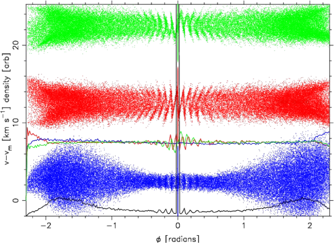
Figure 2.— The angular density distribution (black line at the bottom) and the velocities of a simulation with no sub-halos, as seen from the center of the potential. The velocities are measured relative to the large scale mean values of the stream at that angle. The points show individual particles (blue, bottom, perpendicular to orbital plane; red, middle, radial velocity, and green, top, parallel to the orbital plane) and the lines show the means in angular bins of 1°, with a running mean over 20° subtracted.

A set of n-body simulations to create streams representative of the Phoenix-Hermus stream are done using the techniques described in Carlberg (2016). The models are not matched to either the orbital or sky density data but are intended to explore the range of outcomes in sub-halo filled potentials would give. The model places a King model globular cluster in the the MW2014 potential (Bovy, 2015) at a location of x = 10 kpc, y = 0, and z= 17.32 kpc, that is, a galactocentric radius of 19.5 kpc and an inclination of 60° which is at the observationally determined stream apocenter. No progenitor globular cluster has been identified so the angular phase of the stream is essentially unconstrained. The model cluster is started with a purely tangential velocity (in the y direction) of 178  km s^-1 which gives rise to an orbit with an eccentricity close to the inferred value of 0.05. The King model cluster has a mass of $0.9\times 10^{5}{\rm\,M_{\odot}}$ which is about the lowest mass cluster that will give tidal streams extended enough in angle, which scales as $M^{1/3}$, to provide substantial stream densities in opposite directions on the sky as in the Phoenix-Hermus association. The stream width also scales as $M^{1/3}$, consistent with the 220 pc width that Grillmair (2014) finds for Hermus, which is relatively wide for a globular cluster stream. The model cluster starts with an outer radius of 0.112 kpc which is equal to the nominal tidal radius estimated from the local gravitational acceleration. Exactly filling the tidal radius gives a fairly steady mass loss which totals a modest 11% over an orbital lifetime of 10.7 Gyr. A modest over-filling of the tidal radius will boost the mass loss rate, but those results are not reported here. The simulation uses a shell code (Carlberg, 2015b) which gives the same accuracy as a full n-body code. 500,000 particles are in the initial cluster.

The velocities and densities in the star stream with no perturbing dark matter sub-halos are shown in Figure 2. The density and mean velocities along the stream are measured in 1° bins, where angles are measured relative to the satellite location along a great circle defined by the instantaneous angular momentum vector of the satellite. The velocities are first measured relative to the values that the satellite orbit has at that location. The particles emerge from the inner and outer saddle points in the potential and stream away, offset from the orbit of the satellite. To allow for the offset and other large scale orbital variations we smooth the mean particle velocities with a running average over $\pm$20° which is subtracted from the individual particles to give the offset from the running mean. The running mean becomes noisy at the ends of the stream. Using a smaller window to compute the running mean reduces the end problems, but also artificially suppresses the velocities offsets that sub-halos create. Figure 2 shows significant epicyclic orbit density variations for about four cycles away from the progenitor in both directions, quickly decreasing with distance from the progenitor as differential velocities in the stream cause them to be overlapped on the sky.

4. The Effects of Sub-halos

Sub-halos are added to the MW2014 potential following the prescription of Carlberg (2016). Only the inner 100 kpc of the simulation is filled with sub-halos, with the inner 56 kpc fully populated since there is no value in computing the forces from sub-halos that will never be near the path of the stream. Sub-halos are generated in the mass range $2.7\times 10^{8}{\rm\,M_{\odot}}$ (above which mass sub-halos are very rare) to $2.7\times 10^{5}{\rm\,M_{\odot}}$ (at which mass sub-halos are no longer doing anything significant to a stream). The outcome is a total of about 100 sub-halos in a simulation matched to the Aquarius (Springel et al., 2008) sub-halo distribution. The numbers of sub-halos in 40 realizations range from 57 to 168 for the different realizations from the same distribution. We generate sub-halos with the constraint that the total mass is the expected mass in the selected part of the mass spectrum. This approach does not include an allowance for differences in the sub-halo populations in cosmological dark halos. Ishiyama et al. (2009) find that the fractional variation from one halo to another is about 25% and Chen et al. (2011) find that inside about a tenth of the virial radius the variation from halo to halo is about a factor of 2, up and down relative to the mean. If there were twice as many sub-halos in the region of the simulated stream, then the number of significantly disturbed regions of the stream would exactly double.

Figure 3 shows one of the streams projected onto galactic Cartesian coordinates at the final step of the simulation. Because the progenitor orbit is nearly circular the stream properties do not depend much on the orbital phase of the cluster. The particular moment shown in Figure 3 is not a good match to the present time for the Phoenix-Hermus stream since the progenitor cluster would be readily visible in the northern sky. The stream shows has had an encounter with a massive sub-halo near the end of the trailing stream a few orbits earlier (the progenitor is rotating counter-clockwise) which creates a folded section of stream and a thin trailing segment.

Figure 4 shows the projection of five separate realizations of the stream projected onto the sky. The angles are measured with respect to the instantaneous orbital plane as defined by the total angular momentum vector (which is not a conserved quantity in the MW2014 potential) centered on the location of the progenitor cluster. The plots are offset from one another 0.35 radian. The vertical displacements from the orbital plane of individual particles are multiplied by 5 to increase the visible width of the streams. Near the progenitor the stream particles are young and the epicyclic oscillations of tidal loss dominate. Further down the stream differential orbital velocities across the stream has blurred out the epicyclic features and the streams are old enough that they have suffered a few encounters with sub-halos. The streams vary in width along their length, although this is hard to detect in the presence of substantial foreground. Each simulation has at least one readily visible “gap” in its longitudinal density.

Figure 3.— The final moment of a simulation with sub-halos projected into galactic coordinates. The progenitor is marked with a circle. A massive sub-halo passed through the stream region near x=0, y=1.5, z=2, where one unit is 8 kpc. The upper and right plots have centers offset 5 units.

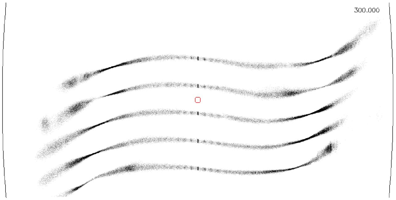
Figure 4.— Five streams plotted along their instantaneous orbital plane as projected onto the sky in an equal area projection. The plots are offset 0.35 radian and extend from over $\pm\pi$. The vertical scale is multiplied by a factor of five to make the width structure visible. The lines at the side are the $\pm\pi$ edges of the coordinate system.

Figure 5 shows the distribution of sub-halo stream encounters at distances from 1 to 3 times the scale radius of the sub-halo, the latter being a somewhat generous distance to produce a significant gap (Carlberg, 2012). The procedure finds the sub-halos closest to a stream particle, relative to its scale radius, at each step. The adopted counting procedure means that lower mass sub-halos are usually not counted when a massive sub-halo is close to the same part of the stream. Figure 5 has 4 mass bins per decade of mass. The most massive sub-halos will typically have one stream hit in the last 3 Gyr during which time the gaps fully develop and remain readily visible.

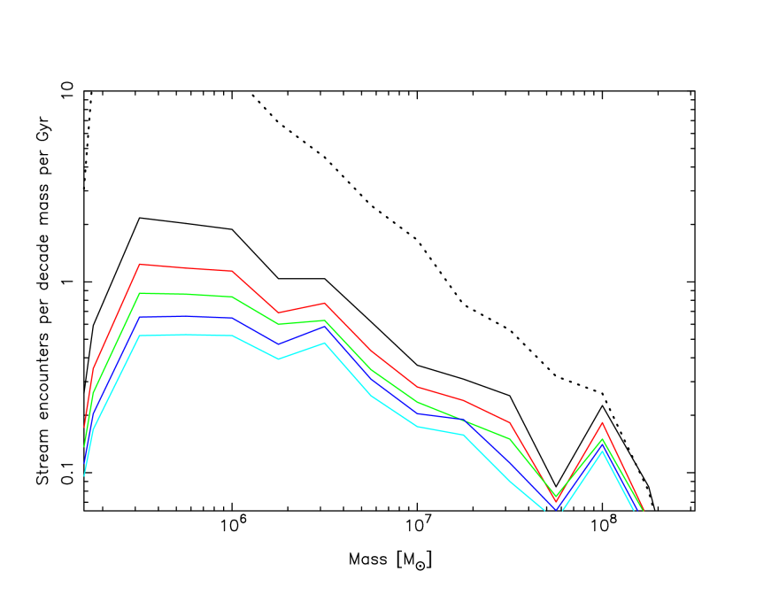
Figure 5.— Rate of stream hits over a 3 Gyr interval starting at 7 Gyr. The rate is shown out to a distance of 1, 1.5, 2, 2.5 and 3 times the scale radius (solid lines from the bottom to the top) of the sub-halo at that mass. The distribution of sub-halo masses is shown as the dotted line. The counting procedure normalizes the distance to the sub-halo scale radius, which leads to the dip near the largest mass bin.

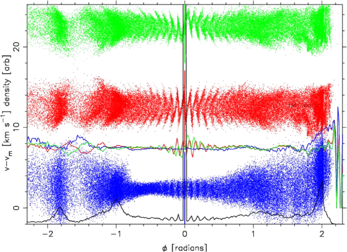
Figure 6.— The same density and velocities plotted as Figure 2 but for a simulation with sub-halos included. Even though the individual particle velocities are scattered on the right hand side (trailing) part of the stream, the mean velocities in projection do not show as large a deviation as the left hand side.

5. Sub-halos and Stream velocity perturbations

Figure 6 shows the same density and velocity measurements as Figure 2 but now for a simulation with sub-halos. Comparing the two shows the effects of the sub-halos on the stream are readily visible beyond about half the stream length, since that is where the stream is old enough to be likely to have had an encounter with one of the heavier sub-halos. The mean radial, parallel and perpendicular velocities are shown as the lines. Radial velocity measurements have no sensitivity to distance errors and are the most likely to be practical in the immediate future. For completeness we also show the local tangential and vertical velocities. If we had access to high precision velocities for many individual stars in the stream the presence (or not) of sub-halos would be obvious. The mean velocities show much smaller effects, with offsets of about 1  km s^-1 around the locations of the large gaps. Only the largest sub-halos, those making gaps 5-10° in size, are readily visible. Small gaps simply do not show up as visible, a consequence of sky overlap of gapped and non-gapped stream regions, and the speed which differential orbital motion, even in this fairly circular orbit, blurs out small gaps.

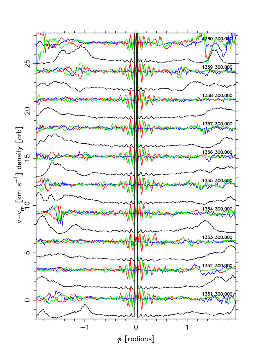
Figure 7.— The same as Figure 6 but with 9 additional realizations of the stream with sub-halos. The black line is the density field and the red, blue and green lines are the radial, local vertical and local tangential velocities, respectively. The figure illustrates the range of mean velocity amplitudes and locations of offsets relative to density variations in the stream.

Figure 7 shows ten different realizations of the same standard sub-halo population to illustrate the range of mean velocity offsets that are exhibited for the same progenitor cluster orbit and different stastical realizations of the sub-halo population. In general if there is a feature that looks like a density gap, with excess density on either side, there is a good chance that there will be velocity offsets associated with it. However, there are exceptions from time to time. This means that a single stream may provide strong evidence of sub-halo encounter, but it will be important to have velocity measurements for as many streams as possible, to allow for case to case differences. Velocities in the plane of the sky perpendicular and along the stream are affected by distance errors, but the means remain unaffected. The stars along the stream contain interesting information about the sub-halo mass, velocity and time of encounter (Erkal & Belokurov, 2015b).

Given the radial velocity signature of a sub-halo encounter, the observational requirement is that to measure reliably an offset from the mean velocity of 1  km s^-1, spread over 10°, with velocities having a peak-to-peak spread of 10  km s^-1 will require individual stellar velocities to be 0.5  km s^-1 or better, for approximately 10 stream stars per degree length of stream. More stars and better velocities will begin to identify the internal structure of the stream, which provides significant additional information on the sub-halo interaction. Detailed modeling for specific observational and stream orbit parameters is straightforward using models similar to those presented here.

The straight line fit to density measurements along the Hermus section of the stream found a decline from the first reliable points to zero over 20° angular extent of stream. Such a steep decline is not seen in the no sub-halo simulation, Figure 2. The ends of the stream have the steepest density decline, but the ends are very artificial, being the result of instantaneously inserting a progenitor star cluster into a Milky Way orbit, rather than some more gradual introduction through, say, a merger process. On the other hand, density declines as steep as measured and more are frequently obtained in simulations with sub-halos, see Figure 6.

6. Discussion

The Phoenix-Hermus stream, whether it is a single object or not, is a good case to consider for sub-halo interactions because the two visible stream segments are long, thin, and appear to be on a relatively circular orbit allowing dark matter sub-halo induced density variations, and associated velocity variations, to remain visible for many orbits before differential orbital motions blur them out. The main point established here is that we expect about one gap per stream to be sufficiently large, about 10°, that there will usually be mean radial velocity offsets of 1-2  km s^-1. Smaller size gaps are present but would require many high precision velocities and dynamical modeling to interpret. The velocity deviation profiles along the stream do not have any simple universal shape and although associated with a density variation, the precise location along the stream relative to a density gap varies fairly uniformly from one edge of a gap to the other over the typical 10° range.

For the expected mean sub-halo population there will be only one easily visible gap present at a time and that gap is the outcome of an encounter of the stream with one of the larger sub-halos, $\approx 10^{8}{\rm\,M_{\odot}}$. Lower mass sub-halos, those below about $10^{7}{\rm\,M_{\odot}}$, generally create gaps and velocity changes that are too small to persist. With only one arm of a stream typically visible, it is possible that no detectable sub-halo effects will be found. However, in the inner halo there is a substantial range for the predicted sub-halo abundance. With the LMC approaching for the first time (Besla et al., 2007) it is possible that its collection of outer sub-halos is currently substantially boosting the numbers of sub-halos in the Milky Way as they stream through on the first infall. For Phoenix-Hermus the ideal is to have a velocity survey everywhere along the stream, but the best locations for finding velocity changes is where the density is changing significantly.

References

- Aaronson (1983) Aaronson, M. 1983, ApJ, 266, L11
- Balbinot et al. (2016) Balbinot, E., Yanny, B., Li, T. S., et al. 2016, ApJ, 820, 58
- Besla et al. (2007) Besla, G., Kallivayalil, N., Hernquist, L., et al. 2007, ApJ, 668, 949
- Bouwens et al. (2015) Bouwens, R. J., Illingworth, G. D., Oesch, P. A., et al. 2015, ApJ, 803, 34
- Bovy (2015) Bovy, J. 2015, ApJS, 216, 29
- Carlberg (2012) Carlberg, R. G. 2012, ApJ, 748, 20
- Carlberg (2013) Carlberg, R. G. 2013, ApJ, 775, 90
- Carlberg (2015a) Carlberg, R. G. 2015a, ApJ, 800, 133
- Carlberg (2015b) Carlberg, R. G. 2015b, ApJ, 808, 15
- Carlberg (2016) Carlberg, R. G. 2016, ApJ, 820, 45
- Chen et al. (2011) Chen, J., Koushiappas, S. M., & Zentner, A. R. 2011, ApJ, 741, 117
- D’Onghia et al. (2010) D’Onghia, E., Springel, V., Hernquist, L., & Keres, D. 2010, ApJ, 709, 1138
- Erkal & Belokurov (2015a) Erkal, D., & Belokurov, V. 2015a, MNRAS, 450, 1136
- Erkal & Belokurov (2015b) Erkal, D., & Belokurov, V. 2015b, MNRAS, 454, 3542
- Erkal et al. (2016) Erkal, D., Belokurov, V., Bovy, J., & Sanders, J. L. 2016, arXiv:1606.04946
- Faber & Lin (1983) Faber, S. M., & Lin, D. N. C. 1983, ApJ, 266, L17
- Grillmair (2014) Grillmair, C. J. 2014, ApJ, 790, L10