A Distributed Algorithm for Training Augmented Complex Adaptive IIR Filters

Abstract

In this paper we consider the problem of decentralized (distributed) adaptive learning, where the aim of the network is to train the coefficients of a widely linear autoregressive moving average (ARMA) model by measurements collected by the nodes. Such a problem arises in many sensor network-based applications such as target tracking, fast rerouting, data reduction and data aggregation. We assume that each node of the network uses the augmented complex adaptive infinite impulse response (ACAIIR) filter as the learning rule, and nodes interact with each other under an incremental mode of cooperation. Since the proposed algorithm (incremental augmented complex IIR (IACA-IIR) algorithm) relies on the augmented complex statistics, it can be used to model both types of complex-valued signals (proper and improper signals). To evaluate the performance of the proposed algorithm, we use both synthetic and real-world complex signals in our simulations. The results exhibit superior performance of the proposed algorithm over the non-cooperative ACAIIR algorithm.

I Introduction

Complex-valued adaptive filters appear in different applications such as communications, power systems, biomedical signal processing and sensor networks [1, 2, 3, 4, 5, 6, 7]. One way to extract a complex-valued adaptive filter algorithm is to extend its real-valued counterpart. The obtained algorithm in this way is suitable only for proper complex-valued signals, since it relies only on the second order statistics, given by the covariance matrix $C_{{\bf xx}}=\mathbb{E}\left[{\bf x}{{\bf x}}^{H}\right]$. By definition, the term circular refers to a complex signal where its probability distribution is rotation-invariant in the complex plane. In addition, the propriety (or second order circularity) implies the second order statistical properties of complex signals [8]. In most real world applications, complex signals are second order noncircular or improper. In order to extract all the available second order information, beside the covariance matrix $C_{{\bf xx}}=\mathbb{E}\left[{\bf x}{{\bf x}}^{H}\right]$, we have to use the pseudocovariance matrix $P_{{\bf xx}}=\mathbb{E}\left[{\bf x}{{\bf x}}^{T}\right]$. To this end, the augmented representation, i.e., ${\bf x}^{a}=[{\bf x}^{T}{\bf x}^{H}]^{T}$ can be used to model the second-order statistical information within the complex domain [9, 10]. The augmented covariance matrix $C_{{\bf xx}}^{a}$ is then given by

$$C_{{\bf xx}}^{a}=\mathbb{E}\left[{\bf x}^{a}{{\bf x}^{a}}^{H}\right]=\left[{\begin{array}[]{*{2}{c}}C_{{\bf xx}}&P_{{\bf xx}}\\ P_{{\bf xx}}^{*}&C_{{\bf xx}}^{*}\end{array}}\right]$$ (1)

Using the augmented representation, it is possible to design widely-linear adaptive algorithms that are able to process proper and improper complex signals [11]. Different complex-valued adaptive filters that rely on the augmented complex statistics have been introduced in the literature such as the widely linear LMS (WL-LMS) [12], augmented CLMS (ACLMS) [13], augmented affine projection algorithm (AAPA) [14], widely linear recursive least squares (WL-RLS) [15], regularized normalized augmented complex LMS (RN-ACLMS) [16], and augmented complex adaptive IIR (ACAIIR) [17].

In this paper we deal with the problem of distributed adaptive learning, where a set of nodes are deployed to collaboratively estimate the coefficients of a widely linear autoregressive moving average (ARMA) model. Such a problem arises in many sensor network-based applications such as target tracking [18, 19], fast rerouting [20, 21], data reduction [22] and data aggregation [23, 24]. To develop our proposed algorithm, we assume that each node uses the ACAIIR filter as the learning rule, and nodes interact with each other under an incremental mode of cooperation. In such a cooperation mode, there exists a cyclic path (Hamilton cycle) among the nods, in which the information goes through the nodes in one direction, i.e. each node passes the information to its adjacent node in a pre-determined direction [25, 26, 27, 28, 29, 30, 31, 32]. To derive the proposed algorithm (incremental augmented complex IIR (IACA-IIR)), we firstly formulate the distributed adaptive learning problem as an unconstrained minimization problem. Then, we use stochastic gradient optimization argument and $\mathbb{CR}$ calculus framework [37] (also known as Wirtinger calculus) to derive a distributed, recursive algorithm to train the complex-valued adaptive IIR filter. We use synthetic complex signal and real-world complex signal in our simulation, where the results reveal that the superior performance of the proposed algorithm, in comparison with the non-cooperative ssolution.

The rest of the paper is organized as follows: in Section II, the IACA-IIR algorithm is derived. In Section III, simulations are presented, and Section IV concludes the paper.

Notation: We adopt small boldface letters for vectors and bold capital letters for matrices. The following notations are adopted: $(\cdot)^{*}$ denotes the complex conjugate, $(\cdot)^{T}$ the transpose of a vector or a matrix, $(\cdot)^{H}$ the Hermitian transpose of a vector or a matrix and $\mathbb{E}\left[\cdot\right]$ represents the statistical expectation.

II Derivation of IACA-IIR Algorithm

Consider an incremental network with $L$ nodes, where each node $k$ has access to data $\{u_{k}(n),{\bf x}_{k}(n)\}$ at time $n$, where ${\bf x}_{k}(n)$ denotes the input vector and

$$u_{k}(n) =d_{k}(n)+v_{k}(n)$$ (2)

where $v_{k}(n)$ denotes the noise term which is assumed as doubly white noise process with variance $\sigma_{v,k}^{2}$. We assume that $v_{k}(n_{1})$ is independent of the input vector ${\mathbf{x}}_{l}(n_{2})$ for all $k\neq l$ and $n_{1}\neq n_{2}$. Moreover, $d_{k}(n)$ (desired signal) is given by the following widely linear model ARMA

$$d_{k}(n) =\sum_{\ell=1}^{M}a^{o}_{\ell}(n)d(n-\ell)+\sum_{\ell=0}^{N}b^{o}_{\ell}(n)x_{k}(n-\ell)+\sum_{\ell=1}^{M}g^{o}_{\ell}(n)d_{k}^{*}(n-\ell)+\sum_{\ell=0}^{N}h^{o}_{\ell}(n)x_{k}^{*}(n-\ell)$$ (3)

where $M>0,\ N>0$ and

$${\mathbf{a}}^{o}=\left[{\begin{array}[]{*{2}{c}}a_{1}\\ a_{2}\\ \vdots\\ a_{M}\end{array}}\right],\ \ {\mathbf{b}}^{o}=\left[{\begin{array}[]{*{2}{c}}b_{0}\\ b_{1}\\ \vdots\\ b_{N}\end{array}}\right],\ \ {\mathbf{g}}^{o}=\left[{\begin{array}[]{*{2}{c}}g_{1}\\ g_{2}\\ \vdots\\ g_{M}\end{array}}\right],\ \ {\mathbf{h}}^{o}=\left[{\begin{array}[]{*{2}{c}}h_{0}\\ h_{1}\\ \vdots\\ h_{N}\end{array}}\right],$$ (20)

are unknown fixed weights. The coefficients of model in (3) can be given at every node $k$ as the output of the following widely linear IIR filter [17]

$$y_{k}(n) =\sum_{m=1}^{M}a_{m,k}(n)y_{k}(n-m)+\sum_{m=0}^{N}b_{m,k}(n)x_{k}(n-m)+\sum_{m=1}^{M}g_{m,k}(n)y_{k}^{*}(n-m)+\sum_{m=0}^{N}h_{m,k}(n)x_{k}^{*}(n-m)$$ (21)

where $\{a_{m},b_{m},g_{m},h_{m}\}$ are complex-valued filter coefficients. To estimate the desired response $d_{k}(n)$ (or equivalently, to train of the complex-valued ARMA model (21)), we can pose the following minimization problem

$$\mathop{\arg\min}\limits_{\{a_{m},b_{m},g_{m},h_{m}\}}J(n)\ \ \mathrm{with}\ \ J(n)\triangleq\sum_{k=1}^{L}|e_{k}(n)|^{2}=\sum_{k=1}^{L}e_{k}(n)e_{k}(n)^{*}$$ (22)

where the corresponding output error at node $k$ is given by

$$e_{k}(n)=d_{k}(n)-y_{k}(n)$$ (23)

Obviously the cost function (22) can be decomposed as $J(n)=\sum_{k=1}^{L}J_{k}(n)$ where $J_{k}(n)=\left|d_{k}(n)-y_{k}(n)\right|^{2}$. Using the traditional iterative steepest-descent algorithm to solve (22) gives

$$\boldsymbol{\phi}(n)=\boldsymbol{\phi}(n-1)-\mu\sum_{k=1}^{L}[\nabla_{\boldsymbol{\phi}(n-1)}J_{k}(n)]^{*}$$ (24)

where $\mu>0$ is the step-size parameter, $\boldsymbol{\phi}(n)$ is a global estimate for ${\mathbf{w}}^{o}=[{\mathbf{a}}^{o},{\mathbf{g}}^{o},{\mathbf{b}}^{o},{\mathbf{h}}^{o}]^{T}$ at iteration $n$, and $\nabla_{\boldsymbol{\phi}(n-1)}$ is the gradient vector of $J_{k}(n)$ with respect to $\boldsymbol{\phi}(n-1)$. Obviously (24) is not a distributed solution as it requires global information $\boldsymbol{\phi}(n)$. To resolve this difficulty, we first introduce the following equivalent implementation for (24) as

$$\left\{\begin{array}[]{l}{\mathbf{w}}_{1}(0)=\boldsymbol{\phi}(n-1)\\ {\mathbf{w}}_{k}(n)={\mathbf{w}}_{k-1}(n)-\mu_{k}[\nabla_{\boldsymbol{\phi}(n-1)}J_{k}(n)]^{*},k=1,2,...,L\\ \boldsymbol{\phi}(n)={\mathbf{w}}_{L}(n)\end{array}\right.$$ (25)

where ${\mathbf{w}}_{k}(n)$ the local estimate of ${\mathbf{w}}^{o}$ at node $k$ and time $n$ . Due to incremental cooperation mode, node $k$ has access to ${\mathbf{w}}_{k-1}(n)$, i.e. an estimate of ${\mathbf{w}}^{o}$ at previous node $k-1$. Thus, to derive a fully distributed solution for (24), we use concept of incremental gradient algorithm [38] and rewrite (25) as

$$\left\{\begin{array}[]{l}{\mathbf{w}}_{1}(0)=\boldsymbol{\phi}(n-1)\\ {\mathbf{w}}_{k}(n)={\mathbf{w}}_{k-1}(n)-\mu_{k}[\nabla_{{\mathbf{w}}_{k-1}(n)}J_{k}(n)]^{*},k=1,2,...,L\\ \boldsymbol{\phi}(n)={\mathbf{w}}_{L}(n)\end{array}\right.$$ (27)

The gradient term is given by

$$\left[\nabla_{{\mathbf{w}}_{k-1}}J_{k}(n)\right]^{*} {}={} -\left[e_{k}(n)\frac{\partial y_{k}^{*}(n)}{\partial{\mathbf{w}}_{k-1}^{*}(n)}+\frac{\partial y_{k}(n)}{\partial{\mathbf{w}}_{k-1}^{*}(n)}e_{k}^{*}(n)\right]$$ (28)

$${}={} -\left[e_{k}(n){\bm{S}}_{{\mathbf{w}}_{k}}(n)+{\bm{P}}_{{\mathbf{w}}_{k}}(n)e_{k}^{*}(n)\right]$$

where the sensitivities ${\bm{S}}_{{\mathbf{w}}_{k}}(n)$ and ${\bm{P}}_{{\mathbf{w}}_{k}}(n)$ are defined as

$${\bm{S}}_{{\mathbf{w}}_{k}}(n)=\frac{\partial y_{k}^{*}(n)}{\partial{\mathbf{w}}_{k-1}^{*}(n)}\Big{|}_{{\mathbf{w}}_{k-1}(n)={\mbox{\footnotesize constant}}}$$ (29)

$${\bm{P}}_{{\mathbf{w}}_{k}}(n)=\frac{\partial y_{k}(n)}{\partial{\mathbf{w}}_{k-1}^{*}(n)}\Big{|}_{{\mathbf{w}}_{k-1}(n)={\mbox{\footnotesize constant}}}$$ (30)

where

$${\bm{S}}_{{\mathbf{w}}_{k}}(n) =[\Phi_{a_{1,k}}(n),...,\Phi_{a_{M,k}}(n),\Phi_{g_{1,k}}(n),...,\Phi_{g_{M,k}}(n),\Phi_{b_{0,k}}(n),...\Phi_{b_{N,k}}(n),\Phi_{h_{0,k}}(n),...,\Phi_{h_{N,k}}(n)]^{T}$$ (31)

$${\bm{P}}_{{\mathbf{w}}_{k}}(n) =[\Psi_{a_{1,k}}(n),...,\Psi_{a_{M,k}}(n),\Psi_{g_{1,k}}(n),...,\Psi_{g_{M,k}}(n),\Psi_{b_{0,k}}(n),...\Psi_{b_{N,k}}(n),\Psi_{h_{0,k}}(n),...,\Psi_{h_{N,k}}(n)]^{T}$$ (32)

We can calculate the gradient in (28) separately. For instance, for $a_{m,k-1}$ we have

$$\frac{\partial y_{k}^{*}(n)}{\partial a_{m,k-1}^{*}(n)} =y_{k}^{*}(n-m)+\sum\limits_{l=1}^{M}a_{l,k-1}^{*}(n)\frac{\partial y_{k}^{*}(n-l)}{\partial a_{m,k-1}^{*}(n)}$$

$$\hskip 28.45274pt+\sum\limits_{l=1}^{M}g_{l,k-1}^{*}(n)\frac{\partial y_{k}(n-l)}{\partial a_{m,k-1}^{*}(n)}$$ (33)

$$\frac{\partial y_{k}(n)}{\partial a_{m,k-1}^{*}(n)} =\sum\limits_{l=1}^{M}a_{l,k-1}(n)\frac{\partial y_{k}(n-l)}{\partial a_{m,k-1}^{*}(n)}$$

$$\hskip 28.45274pt+\sum\limits_{l=1}^{M}g_{l,k-1}(n)\frac{\partial y_{k}^{*}(n-l)}{\partial a_{m,k-1}^{*}(n)}$$ (34)

As we can see from (33) and (34), to calculate the gradient in (28) we need to compute the derivatives $\frac{\partial y_{k}^{*}(n-l)}{\partial a_{m,k-1}^{*}(n)}$ for $l=1,2,\cdots,M$, which is not possible. To circumvent this issue, we consider the following approximation for a small convergence rate $\mu$ [39]:

$${\mathbf{w}}_{k}(n) \approx{\mathbf{w}}_{k}(n-1)\approx...\approx{\mathbf{w}}_{k}(n-\tau)$$ (35)

where $\tau=max\{M,N+1\}$. Thus, the relations (33) and (34) can be approximated as follows

$$\frac{\partial y_{k}^{*}(n)}{\partial a_{m,k-1}^{*}(n)} =y_{k}^{*}(n-m)+\sum\limits_{l=1}^{M}a_{l,k-1}^{*}(n)\frac{\partial y_{k}^{*}(n-l)}{\partial a_{m,k-1}^{*}(n-l)}$$

$$\hskip 28.45274pt+\sum\limits_{l=1}^{M}g_{l,k-1}^{*}(n)\frac{\partial y_{k}(n-l)}{\partial a_{m,k-1}^{*}(n-l)}$$ (36)

$$\frac{\partial y_{k}(n)}{\partial a_{m,k-1}^{*}(n)} =\sum\limits_{l=1}^{M}a_{l,k-1}(n)\frac{\partial y_{k}(n-l)}{\partial a_{m,k-1}^{*}(n-l)}$$

$$\hskip 28.45274pt+\sum\limits_{l=1}^{M}g_{l,k-1}(n)\frac{\partial y_{k}^{*}(n-l)}{\partial a_{m,k-1}^{*}(n-l)}$$ (37)

Since delayed version of sensitivities appearing in the right hand side of above relations, the sensitivities can be written as

$$\Phi_{a_{m,k}}(n) =y_{k}^{*}(n-m)+\sum\limits_{l=1}^{M}a_{l,k-1}^{*}(n)\Phi_{a_{m,k}}(n-l)$$

$$\hskip 28.45274pt+\sum\limits_{l=1}^{M}g_{l,k-1}^{*}(n)\Psi_{a_{m,k}}(n-l)$$ (38)

$$\Psi_{a_{m,k}}(n) =\sum\limits_{l=1}^{M}a_{l,k-1}(n)\Psi_{a_{m,k}}(n-l)$$

$$\hskip 28.45274pt+\sum\limits_{l=1}^{M}g_{l,k-1}(n)\Phi_{a_{m,k}}(n-l)$$ (39)

Similarly, update relations for other sensitivities can be obtained as

$$\Phi_{g_{m,k}}(n) =y_{k}(n-m)+\sum\limits_{l=1}^{M}a_{l,k-1}^{*}(n)\Phi_{g_{m,k}}(n-l)$$

$$\hskip 34.14322pt+\sum\limits_{l=1}^{M}g_{l,k-1}^{*}(n)\Psi_{g_{m,k}}(n-l)$$ (40)

$$\Phi_{b_{m,k}}(n) =x_{k}^{*}(n-m)+\sum\limits_{l=1}^{M}a_{l,k-1}^{*}(n)\Phi_{b_{m,k}}(n-l)$$

$$\hskip 34.14322pt+\sum\limits_{l=1}^{M}g_{l,k-1}^{*}(n)\Psi_{b_{m,k}}(n-l)$$ (41)

$$\Phi_{h_{m,k}}(n) =x_{k}(n-m)+\sum\limits_{l=1}^{M}a_{l,k-1}^{*}(n)\Phi_{h_{m,k}}(n-l)$$

$$\hskip 34.14322pt+\sum\limits_{l=1}^{M}g_{l,k-1}^{*}(n)\Psi_{h_{m,k}}(n-l)$$ (42)

And also we have

$$\Psi_{g_{m,k}}(n) =\sum\limits_{l=1}^{M}a_{l,k-1}(n)\Psi_{g_{m,k}}(n-l)$$

$$\hskip 34.14322pt+\sum\limits_{l=1}^{M}g_{l,k-1}(n)\Phi_{g_{m,k}}(n-l)$$ (43)

$$\Psi_{b_{m,k}}(n) =\sum\limits_{l=1}^{M}a_{l,k-1}(n)\Psi_{b_{m,k}}(n-l)$$

$$\hskip 34.14322pt+\sum\limits_{l=1}^{M}g_{l,k-1}(n)\Phi_{b_{m,k}}(n-l)$$ (44)

$$\Psi_{h_{m,k}}(n) =\sum\limits_{l=1}^{M}a_{l,k-1}(n)\Psi_{h_{m,k}}(n-l)$$

$$\hskip 34.14322pt+\sum\limits_{l=1}^{M}g_{l,k-1}(n)\Phi_{h_{m,k}}(n-l)$$ (45)

In above relations, we need to update $4(M+N+1)$ sensitivities, but we can reduce the number of update relations to only eight update relations by using the approximation (35). For instance, for term

$${c}\Phi_{a_{k}}(n)=[\Phi_{a_{1,k}}(n),\Phi_{a_{2,k}}(n),...,\Phi_{a_{M,k}}(n)]^{T}$$ (46)

We have

$$\Phi_{a_{2,k}}(n)=y_{k}^{*}(n-2)+\sum\limits_{l=1}^{M}a_{l,k-1}^{*}(n)\Phi_{a_{2,k}}(n-l)$$

$$+\sum\limits_{l=1}^{M}g_{l,k-1}^{*}(n)\Psi_{a_{2,k}}(n-l)$$ (47)

That can be replaced with

$$\Phi_{a_{2,k}}(n) {}={} \Phi_{a_{1,k}}(n-1)$$ (48)

$${}={} y_{k}^{*}(n-1-1)+\sum\limits_{l=1}^{M}a_{l,k-1}^{*}(n-1)\Phi_{a_{1,k}}(n-1-l)$$

$$+\sum\limits_{l=1}^{M}g_{l,k-1}^{*}(n-1)\Psi_{a_{1,k}}(n-1-l)$$

$${}={} y_{k}^{*}(n-2)+\sum\limits_{l=1}^{M}\underbrace{a_{l,k-1}^{*}(n-1)}_{\mbox{\footnotesize time delayed version}}\Phi_{a_{2,k}}(n-l)$$

$${+}\>\sum\limits_{l=1}^{M}\underbrace{g_{l,k-1}^{*}(n-1)}_{\mbox{\footnotesize time delayed version}}\Psi_{a_{2,k}}(n-l)$$

This approximation can be applied to all other sensitivities. Finally, the update relations for weight vectors in the compact form is given by

$${\mathbf{w}}_{k}(n)={\mathbf{w}}_{k-1}(n)+\mu_{k}[e_{k}(n){\bm{S}}_{{\mathbf{w}}_{k}}(n)+{\bm{P}}_{{\mathbf{w}}_{k}}(n)e_{k}^{*}(n)]$$ (49)

This completes the derivation of the proposed IACA-IIR algorithm.

III Simulations

In order to evaluate the proposed algorithm and to compare it with the non-cooperative case, we consider different complex-valued signals in one-step Ahead prediction setting. One synthetic signal is a stable and circular complex valued AR(4) process used is given by

$$r(n)=1.79r(n-1)-1.85r(n-2)+1.27r(n-3)-0.41r(n-4)+z(n)$$ (50)

where $z(n)$ denotes doubly white proper noise with unit variance. The other test signal is a linear MA which is a proper process which is described by [40]:

$$y(0) {}={} 0$$

$$y(n) {}={} 2z(n)+0.5z^{*}(n)+z(n-1)$$ (51)

$$+0.9z^{*}(n-1),n\geq 1$$

Other synthetic signal is a linear ARMA which is a improper process and is defined as a combination of MA process (III) and AR process, that is given by [41]:

$$r(0) {}={} 0$$

$$r(n) {}={} 1.8r(n-1)-1.85r(n-2)$$ (52)

$$+1.3r(n-3)-0.5r(n-4)$$

$$+0.22r(n-5)+2z(n)+0.5z^{*}(n)$$

$$+z(n-1)+0.9z^{*}(n-1),n\geq 1$$

with

$$\mathbb{E}\left[z(n-n_{1})z^{*}(n-n_{2})\right]=\delta(n_{1}-n_{2})$$

$$\mathbb{E}\left[z(n-n_{1})z(n-n_{2})\right]=\lambda\delta(n_{1}-n_{2})$$ (53)

where $z(n)$ denotes doubly white proper noise, and $\lambda$ shows the noncircularity degree of signal. With $\lambda=0$, the proper MA model is achieved and with $\lambda=0.95$, the improper ARMA model is achieved. The third complex-valued signal is a real-world 2-D wind process which is considered to have medium dynamic. Fig. 1 shows the scatter plots of the mentioned complex signals.

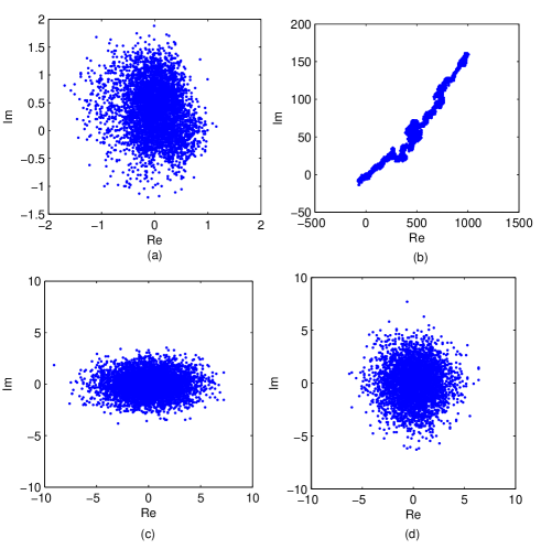
Figure 1: Scatter plots for complex signals used in our simulations (a) circular complex valued AR(4) process, (b) Proper MA process, (c) improper ARMA process, and (d) complex wind signal.

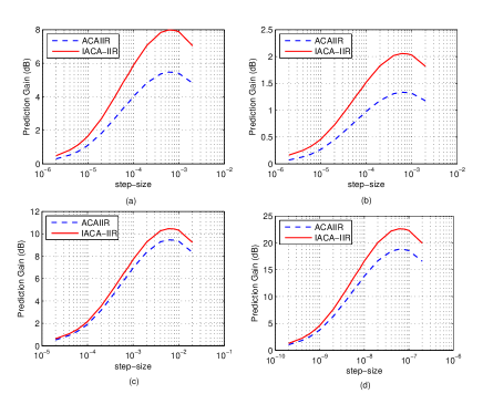
Figure 2: Performance comparison between ACAIIR and IACA-IIR for prediction of (a) circular complex valued AR(4) process, (b) Proper MA process, (c) improper ARMA process, and (d) complex wind signal.

The network has $L=10$ nodes, and the filter order is set to $M=N=4$, that $M$ and $N$ denote respectively the order of feedback and feedforward of the filter. In order to evaluating the performance, the prediction gain $R_{p}=10\log(\sigma_{x}^{2}/\sigma_{e}^{2})$ is used, where $\sigma_{x}^{2}$ and $\sigma_{e}^{2}$ are respectively the variance of the input and output error.

Fig.  2 illustrates the performance of proposed algorithm for prediction of complex-valued signals of interest and compares it with non-cooperative case over a range of step-size parameters. It can be observed that, in all situations, the proposed IACA-IIR algorithm outperforms the non-cooperative case. For a very small step size values, the adaptive algorithm can not track the signal (in prediction setting) and therefore the output variance is high (prediction gain is low). As step size increases, the ability of algorithm to follow the signal improves and the output variance decreases (prediction gain increases). Finally for large step sizes, the output error increases again and prediction gain decreases.

Fig.  3 illustrates the MSE curves of ACAIIR and IACA-IIR algorithms for prediction of circular complex valued AR(4) signal, and improper ARMA model. The step size parameters are set to $\mu=10^{-3}$ (for circular complex valued AR(4) signal) and $\mu=10^{-7}$ (for improper ARMA model). It can be observed that, in this situation, the proposed IACA-IIR algorithm possesses faster convergence and smaller MSE than non-cooperative case. The impact of network size on the performance of the proposed (in terms of the prediction gain) for wind signal (for $\mu=10^{-6}$) is shown in Fig. 4. We can see that increasing the network size improves the performance of the proposed algorithm.

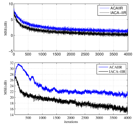
Figure 3: Comparison of MSEs of ACAIIR and IACA-IIR for prediction of (top) circular complex valued AR(4) process, and (bottom) improper ARMA model.

IV Conclusion

In this paper we derive a distributed adaptive learning algorithm for training augmented complex adaptive IIR filters. The proposed algorithm (IACA-IIR) relies on the augmented complex statistics and incremental cooperation mode. We used both synthetic and real-world circular and noncircular signals to evaluate the performance of the proposed algorithm, where the results reveal its superior performance over the non-cooperative ACAIIR algorithm. In our future work we plan to study the stability conditions for the proposed algorithm, especially in the different communications scenarios such as networks with noisy links.

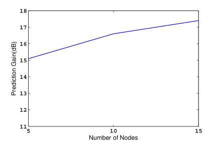
Figure 4: The impact of network size on the performance of the proposed (in terms of the prediction gain) for wind signal.

References

- [1] B. Picinbono and P. Chevalier, “Widely linear estimation with complex data,” IEEE Transactions on Signal Processing, vol. 43, no. 8, pp. 2030–2033, Aug 1995.
- [2] T. Adali, P. Schreier, and L. Scharf, “Complex-valued signal processing: The proper way to deal with impropriety,” Signal Processing, IEEE Transactions on, vol. 59, no. 11, pp. 5101–5125, Nov 2011.
- [3] A. Khalili, A. Rastegarnia, and W. Bazzi, “A collaborative adaptive algorithm for the filtering of noncircular complex signals,” in Telecommunications (IST), 2014 7th International Symposium on, Sept 2014, pp. 96–99.
- [4] Y. Xia, D. Mandic, and A. Sayed, “An adaptive diffusion augmented clms algorithm for distributed filtering of noncircular complex signals,” Signal Processing Letters, IEEE, vol. 18, no. 11, pp. 659–662, Nov 2011.
- [5] S. Kanna, S. Talebi, and D. Mandic, “Diffusion widely linear adaptive estimation of system frequency in distributed power grids,” in Energy Conference (ENERGYCON), 2014 IEEE International, May 2014, pp. 772–778.
- [6] C. Jahanchahi and D. Mandic, “An adaptive diffusion quaternion lms algorithm for distributed networks of 3d and 4d vector sensors,” in Signal Processing Conference (EUSIPCO), 2013 Proceedings of the 21st European, Sept 2013, pp. 1–5.
- [7] A. Khalili, A. Rastegarnia, and S. Sanei, “Robust frequency estimation in three-phase power systems using correntropy-based adaptive filter,” IET Science, Measurement and Technology, vol. 9, no. 8, pp. 928-935, Nov. 2015, doi: 10.1049/iet-smt.2015.0018.
- [8] B. Picinbono, “On circularity,” IEEE Transactions on Signal Processing, vol. 42, no. 12, pp. 3473–3482, Dec 1994.
- [9] F. Neeser and J. Massey, “Proper complex random processes with applications to information theory,” IEEE Transactions on Information Theory, vol. 39, no. 4, pp. 1293–1302, Jul 1993.
- [10] B. Picinbono, “Second-order complex random vectors and normal distributions,” IEEE Transactions on Signal Processing, vol. 44, no. 10, pp. 2637–2640, Oct 1996.
- [11] D. Mandic and V. S. L. Goh, Complex Valued Nonlinear Adaptive Filters: Noncircularity, Widely Linear and Neural Models. Wiley Publishing, 2009.
- [12] R. Schober, W. Gerstacker, and L. H.-J. Lampe, “Data-aided and blind stochastic gradient algorithms for widely linear mmse mai suppression for ds-cdma,” Signal Processing, IEEE Transactions on, vol. 52, no. 3, pp. 746–756, March 2004.
- [13] S. Javidi, M. Pedzisz, S. L. Goh, and D. P. Mandic, “The augmented complex least mean square algorithm with application to adaptive prediction problems,” in 1st IARP Workshop Cogn. Inform. Process., 2008, pp. 54–57.
- [14] Y. Xia, C. CheongTook, and D. P. Mandic, “An augmented affine projection algorithm for the filtering of noncircular complex signals,” Signal Processing, vol. 90, no. 6, pp. 1788 – 1799, 2010.
- [15] S. Douglas, “Widely-linear recursive least-squares algorithm for adaptive beamforming,” in Acoustics, Speech and Signal Processing, 2009. ICASSP 2009. IEEE International Conference on, April 2009, pp. 2041–2044.
- [16] Y. Xia, S. Javidi, and D. Mandic, “A regularised normalised augmented complex least mean square algorithm,” in Wireless Communication Systems (ISWCS), 2010 7th International Symposium on, Sept 2010, pp. 355–359.
- [17] C. Took and D. Mandic, “Adaptive iir filtering of noncircular complex signals,” IEEE Transactions on Signal Processing, vol. 57, no. 10, pp. 4111–4118, Oct 2009.
- [18] X. Wang, S. Wang, J.-J. Ma, and D.-W. Bi, “Energy-efficient organization of wireless sensor networks with adaptive forecasting,” Sensors, vol. 8, no. 4, pp. 2604–2616, 2008.
- [19] X. Wang, S. Wang, D.-W. Bi, and J.-J. Ma, “Distributed peer-to-peer target tracking in wireless sensor networks,” Sensors, vol. 7, no. 6, pp. 1001–1027, 2007. [Online]. Available: http://www.mdpi.com/1424-8220/7/6/1001
- [20] Z. Li, J. Bi, and S. Chen, “Traffic prediction-based fast rerouting algorithm for wireless multimedia sensor networks, international journal of distributed sensor networks,” International Journal of Distributed Sensor Networks, vol. 2013, no. 7, p. 11 pages, 2013.
- [21] H. Gharavi and B. Hu, “Cooperative diversity routing and transmission for wireless sensor networks,” Wireless Sensor Systems, IET, vol. 3, no. 4, pp. 277–288, December 2013.
- [22] M. Mohamed, W. Wu, and M. Moniri, “Data reduction methods for wireless smart sensors in monitoring water distribution systems,” Procedia Engineering, vol. 70, no. 0, pp. 1166 – 1172, 2014, 12th International Conference on Computing and Control for the Water Industry, {CCWI2013}.
- [23] J. Lu, F. Valois, M. Dohler, and M.-Y. Wu, “Optimized data aggregation in wsns using adaptive arma,” in Sensor Technologies and Applications (SENSORCOMM), 2010 Fourth International Conference on, July 2010, pp. 115–120.
- [24] H. Harb, A. Makhoul, R. Tawil, and A. Jaber, “Energy-efficient data aggregation and transfer in periodic sensor networks,” Wireless Sensor Systems, IET, vol. 4, no. 4, pp. 149–158, 2014.
- [25] M. Rabbat and R. Nowak, “Quantized incremental algorithms for distributed optimization,” IEEE Journal on Selected Areas in Communications, vol. 23, no. 4, pp. 798–808, April 2005.
- [26] C. Lopes and A. Sayed, “Incremental adaptive strategies over distributed networks,” IEEE Transactions on Signal Processing, vol. 55, no. 8, pp. 4064–4077, Aug 2007.
- [27] Y. Liu and W. K. Tang, “Enhanced incremental {LMS} with norm constraints for distributed in-network estimation,” Signal Processing, vol. 94, no. 0, pp. 373 – 385, 2014.
- [28] M. S. E. Abadi and A.-R. Danaee, “Low computational complexity family of affine projection algorithms over adaptive distributed incremental networks,” {AEU} - International Journal of Electronics and Communications, vol. 68, no. 2, pp. 97 – 110, 2014.
- [29] A. Rastegarnia and A. Khalili, “Incorporating observation quality information into the incremental lms adaptive networks,” Arabian Journal for Science and Engineering, vol. 39, no. 2, pp. 987–995, 2014.
- [30] A. Khalili, A. Rastegarnia, W. Bazzi, and Z. Yang, “Derivation and analysis of incremental augmented complex least mean square algorithm,” Signal Processing, IET, vol. 9, no. 4, pp. 312–319, 2015.
- [31] A. Khalili, A. Rastegarnia, and W. Bazzi, “Incremental augmented affine projection algorithm for collaborative processing of complex signals,” in Information and Communication Technology Research (ICTRC), 2015 International Conference on, May 2015, pp. 60–63.
- [32] R. G. Rahmati, A. Khalili, A. Rastegarnia, and H. Mohammadi, “An adaptive incremental algorithm for distributed filtering of hypercomplex processes,” American Journal of Signal Processing, vol. 5, no. (2A), pp. 9–15, 2015.
- [33] A. H. Sayed, S.-Y. Tu, J. Chen, X. Zhao, and Z. Towfic, “Diffusion strategies for adaptation and learning over networks,” IEEE Signal Processing Magazine, vol. 30, no. 3, pp. 155–171, May 2013.
- [34] C. Lopes and A. Sayed, “Diffusion least-mean squares over adaptive networks: Formulation and performance analysis,” Signal Processing, IEEE Transactions on, vol. 56, no. 7, pp. 3122–3136, 2008.
- [35] F. Cattivelli and A. Sayed, “Diffusion lms strategies for distributed estimation,” Signal Processing, IEEE Transactions on, vol. 58, no. 3, pp. 1035–1048, 2010.
- [36] R. Abdolee, B. Champagne, and A. H. Sayed, “Diffusion LMS strategies for parameter estimation over fading wireless channels,” in Proc. IEEE Int. Conf. on Communications, Jun. 2013.
- [37] K. Kreutz-Delgado, “The Complex Gradient Operator and the -Calculus,” Lecture Suppl. ECE275A, pp. 1–74, 2006.
- [38] J. Tsitsiklis, D. Bertsekas, and M. Athans, “Distributed asynchronous deterministic and stochastic gradient optimization algorithms,” Automatic Control, IEEE Transactions on, vol. 31, no. 9, pp. 803–812, Sep 1986.
- [39] J. R. Treichler, C. R. Johnson, Jr., and M. J. Larimore, Theory and Design of Adaptive Filters. New York, NY, USA: Wiley-Interscience, 1987.
- [40] J. Navarro-Moreno, “Arma prediction of widely linear systems by using the innovations algorithm,” IEEE Transactions on Signal Processing, vol. 56, no. 7, pp. 3061–3068, July 2008.
- [41] D. P. Mandic and J. A. Chambers, Recurrent Neural Networks for Prediction. New York: Wiley, 2001.