Canonical transfer and multiscale energetics for primitive and quasi-geostrophic atmospheres

Abstract

The past years have seen the success of a novel multiscale energetics formalism in a variety of ocean and engineering fluid applications. In a self-contained way, this study introduces it to the atmospheric dynamical diagnostics, with important theoretical updates. Multiscale energy equations are derived using a new analysis apparatus, namely, multiscale window transform, with respect to both the primitive equation and quasi-geostrophic models. A reconstruction of the “atomic” energy fluxes on the multiple scale windows allows for a natural and unique separation of the in-scale transports and cross-scale transfers from the intertwined nonlinear processes. The resulting energy transfers bear a Lie bracket form, reminiscent of the Poisson bracket in Hamiltonian mechanics; we hence would call them “canonical”. A canonical transfer process is a mere redistribution of energy among scale windows, without generating or destroying energy as a whole. By classification, a multiscale energetic cycle comprises of available potential energy (APE) transport, kinetic energy (KE) transport, pressure work, buoyancy conversion, work done by external forcing and friction, and the cross-scale canonical transfers of APE and KE which correspond respectively to the baroclinic and barotropic instabilities, among others, in geophysical fluid dynamics. A buoyancy conversion takes place in an individual window only, bridging the two types of energy namely KE and APE; it does not involve any processes among different scale windows, and is hence basically not related to instabilities. This formalism is exemplified with a preliminary application to the Madden-Julian Oscillation study.

I Introduction

Ever since Lorenz (1955)Lorenz introduced the concept of available potential energy (APE), and set up a two-scale formalism of energy equations using the Reynolds decomposition, energetic analysis has become a powerful tool for diagnosing atmospheric and oceanic processes. Related studies include mean flow-wave interaction (e.g., Dickinson , Boyd , McWilliams99 , Fels_Lindzen , Matsuno ), upward propagation of planetary-scale disturbances (Charney ), ocean circulation energetics (Holland , Haidvogel ), mean current-eddy interaction (Hoskins ), atmospheric blocking (Trenberth , Fournier , Luo ), Gulf Stream dynamics (Dewar ), normal modal interaction (Sheng90 ), regional cyclogenesis (Cai90 ), convection and cabbeling (Ingersoll16 ), and the most recent studies such as Cai07 , Waterman , Murakami11 , Hsu , Chen , Chapman , to name a few. Meanwhile, SaltzmanSaltzman57 cast the problem into the framework of Fourier analysis, and obtained the energetics in the wavenumber domain, while KaoKao further extended it to the wavenumber-frequency space. Now both approaches have become standard in geophysical fluid dynamics and other fluid-related fields; see, for example, Pedlosky , Chorin , Pope , etc.

Lorenz’ energetics in bulk form, i.e., in the form of global mean or integral, have clear physical interpretations (e.g., Pedlosky ). This global mean form, however, may be inappropriate for regional diagnostics, as real atmospheric processes are localized in nature; in other words, they tend to be locally defined in space and time, and can be on the move. The Madden-Julian Oscillation (MJO) that we will take a brief look at the end of this study is such an example; it is a progressive process that involves energy production and dissipation. For this reason, it has been a continuing effort to relax the spatial averaging/integration to have these processes faithfully represented. A tradition started by Lorenz himself is to collect the terms in divergence form and combine them as one term representing the transport process, separate the term from the nonlinear interaction and take the residue as the energy transfer between the distinct scales (e.g., Harrison ). Now this has been a standard approach to multiscale energetic diagnostics for fluid research, particularly for turbulence research, where much effort has been devoted to engineering the so-obtained transfers (cf. Pope ).

While we know a transport process indeed bears a divergence form in the governing equations, the above transport-transfer separation is not unique. Multiple divergence forms exist that may yield quite different transfers. As argued by Holopainen (1978), the resulting energy transfer in such an open system is quite ambiguous. This issue, which is actually much profound in fluid dynamics, has long been discovered, but have not received enough attention, except for a few studies such as Plumb83 . (The author was just aware of Berloff’s discussion on the consistency of eddy fluxesBerloff , which also seems to be related to this problem.)

Another major issue in formulating multiscale energetics regards the machinery for process decomposition by scale. Traditionally two methods, namely, Reynolds’ mean-eddy decomposition (MED) and Fourier transform, have been used. The former is originally a statistical notion with respect to an ensemble mean, but for practical reason the ensemble mean is usually replaced by time mean, zonal mean, etc., making it a tool of scale decomposition. Both these methods are global, in the sense that they do not retain the local information. This is generally inappropriate for realistic atmospheric processes such as instabilities, which are in nature highly localized energy burst processes. In remedy, a practical approach that is commonly used is to do running time mean over a chosen duration of time. Indeed this gives the local information while retaining the simplicity of the Reynolds formalism. However, it does not solve the fundamental problem that an energy burst process, among others, is by no means stationary over any duration; any scale decomposition under such a hidden assumption may result in spurious information, preventing one from making correct diagnoses.

An alternative approach to overcoming the difficulty is via filtering. Filters have been widely used to separate processes involving different scales. But for energetics studies, it seems that a very fundamental issue has been completely ignored, that is, how energy (and any quadratic properties) should be expressed in this framework. Currently the common practice is, for a two-scale decomposition, to first apply some filter to separate a field variable, say, $u$, into two parts, say, $u_{L}$ and $u_{S}$, which represent the large-scale and small-scale features, and then take $u_{L}^{2}$ and $u_{S}^{2}$ (up to some factor) as the large-scale and small-scale energies. While this intuitively based and widely used technique may be of some use in real problem diagnostics, it is not physically relevant—one immediately sees the inadequacy by noticing that $u^{2}\neq u_{L}^{2}+u_{S}^{2}$. In fact, multiscale energy is a concept in phase space, such as that in Fourier power spectra; it is related to physical energy through a theorem called Parseval relation. Attempting to evaluate multiscale energies with the filtered (low-pass, band-pass, etc.) or reconstructed field variables is conceptually off track. Actually this is a difficult problem, and has not been well formulated until filter banks and wavelets are connected (Strang ). Besides, energy conservation requires that the resulting subspaces from filtering must be orthogonal, as we will elaborate in the following section. This requirement, unfortunately, has been mostly ignored in previous studies along this line.

The other line in this regard is with respect to Fourier transform (Saltzman57 , and the sequels), which does not have local information retained, either. Coming to remedy is wavelet transform or, to be precise, orthonormal wavelet transform (OWT), as only with an orthogonal basis can the notion of energy in the physical sense be introduced. In 2000, Fournier first introduced OWT into the study of atmospheric energetics. This is a formalism with respect to space. While opening a door to localized spectral structures, many processes such as transports are not as easy to see as those in the Lorenz-type formalisms. On the other hand, the atmospheric and oceanic processes tend to occur on a ranges of scales (e.g., MJO has a scale range of 30-60 days), or scale windows as we will introduce in the following section, rather than on individual scales. For OWT, transform coefficients (hence multiscale energies) are defined discretely at different locations for different scale levels; there is no way to add them through a range of scales to make an expression of localized energy for that range. These issues, among others, are yet to be addressed with these formalisms.

So, to relax the spatial averaging in a bulk energetics formalism incurs the issue of transport-transfer separation, while to improve the MED to have local information retained requires a more sophisticated machinery of scale decomposition. Can we put these two issues in the same framework and solve them in a unified approach? The answer is yes. The early attempts include the multiscale oceanic energetics studies by Liang and Robinson (2005)LR05 (LR05 henceforth), based on multiscale window transform (MWT), a functional analysis tool which was rigorized later (Liang and Anderson 2007LA07 , LA07 hereafter). This formalism has been mostly overlooked, though it has been applied with success to a variety of real ocean problems (e.g., LR04, LR09 ) and engineering problems (e.g., Liang_Wang ), partly because it has not been introduced for atmospheric studies, and has not been formulated in spherical coordinates. (As we will see soon, expressing the energetics in spherical coordinates is by no means an easy task.) This study is purported to address these issues, giving a comprehensive and self-contained introduction of the fundamentals and the progress since LR05. A key point that distinguishes this study from the earlier effort is that, in LR05, the transport-transfer separation was introduced in a half-empirical way. With the nice properties of the MWT which was formally established later on in LA07, we will see soon in the next section that this actually can be put on a rigorous footing, and the resulting transfer bears a Lie bracket form, reminding us of the Poisson bracket in Hamiltonian mechanics. Besides, in this study we will extend the formalism to quasi-geostrophic flows, which must be derived in a different way. Considering the traditional and recently renewed interests (e.g., Murakami11 ) in multiscale atmospheric energetics diagnostics, and considering that a topic of much concern in turubulence research is to engineer the resulting transfer, this rigorous study is rather timely.

In the following we first give a brief introduction of the concepts of scale window, multiscale window transform, and multiscale energy. In §III, we show that how the flux on a specific scale window can be rigorously derived, and how the energy transfer between two scale windows can be obtained. We will see that the resulting transfer bears a form like Lie bracket, reminding one of the Poisson bracket in Hamiltonian dynamics. We then derive the evolution equations for the multiscale kinetic energy (KE) and available potential energy (APE) with both a primitive atmospheric model (§IV) and a quasi-geostrophic model (§VI). For completeness, a summary of the multiscale oceanic energetics, together with the needed modification, is briefly presented (§V); also included is a brief review of some necessary horizontal treatment (§VII). In section VIII, we demonstrate how the formalism may be applied, using the Madden-Julian Oscillation as an example. This study is summarized in §IX. For easy reference, in appendix A a glossary of symbols is provided. The related software can be downloaded from the website http://www.ncoads.org/ (within the section “Software”).

II Multiscale window transform

This section gives a very brief introduction of the multiscale window transform developed by LA07. The first part (§II.1) is the fundamentals; but the reader may simply skip it if he/she already knows the notation and the fact that a reconstruction is conceptually different from a transform.

II.1 Scale window and multiscale window transform

More often than not, an atmospheric process tends to occur on a range of scales, such as the MJO which has a broadband spectrum between 30 and60 days (cf. section VIII), rather than on individual scales. Such a scale range is called, in a loose sense, a scale window. Rigorously it can be defined over a univariate interval or a multi-dimensional domain. In this study, the former is used, as we only deal with time. This is in accordance with Lorenz’ formalism. Historically it has long been discussed (e.g., Haynes ), and has been justified by the observational fact that, in the atmosphere, scales in time and in space are correlated. Besides, only scales defined over a univariate field can be unambiguously referred to as large scale, small scale, and so forth, as desired in the atmospheric energetics studies.

Without loss of generality, let the interval over which the signals to be diagnosed span be $[0,1]$; if not, it may always be made so after a transformation. Consider a Hilbert space $V_{{\ell},j}\subset L_{2}[0,1]$ generated by the basis $\{\phi_{n}^{j}(t)\}_{n=0,1,...,2^{j}{\ell}-1}$, where

$$\phi_{n}^{j}(t)=\sum_{q=-\infty}^{+\infty}2^{j/2}\phi[2^{j}(t+{\ell}q)-n+1/2],\qquad n=0,1,...,2^{j{\ell}-1}.$$ (1)

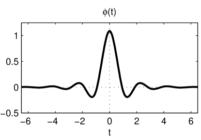
Figure 1: The orthonormal scaling function $\phi$ constructed in LA07 .

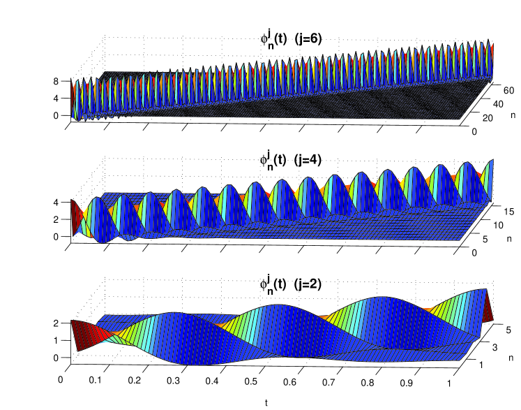
Figure 2: $\phi_{n}^{j}$ as function of $t$ (physical space variable; here time) and $n$ (sampling space variable) for a selection of scale level $j$ (corresponding to scale $2^{-j}$ on a [0,1] domain). The symmetric extension scheme is used in constructing $\phi_{n}^{j}$ via the $\phi$ in Fig. 1.

Here $\phi(t)$ is a scaling function constructed in LA07 such that $\{\phi(t-n+1/2)\}_{n}$ is orthonormal (Fig. 1). From $\phi(t)$ one can also construct an orthonormal wavelet basis. The parameter ${\ell}=1$ or ${\ell}=2$, corresponding respectively to the periodic and symmetric extension schemes. Shown in Fig. 2 is the basis for ${\ell}=2$ and a selection of $j$, namely, the “scale level” ($2^{-j}$ is the scale). For notational simplicity, throughout this study the dependence of $\phi_{n}^{j}$ on ${\ell}$ is suppressed (but retained in other notations).

It has been justified in LA07 that there always exists a $j_{2}$ such that all the atmospheric/oceanic signals of concern lie in $V_{{\ell},j_{2}}$. Furthermore, it has been shown in there that

$$V_{{\ell},j_{0}}\subset V_{{\ell},j_{1}}\subset V_{{\ell},j_{2}},\qquad{\rm for}\ j_{0}<j_{1}<j_{2}.$$

A decomposition thus can be made such that

$$V_{{\ell},j_{2}}=V_{{\ell},j_{1}}\oplus W_{{\ell},j_{1}-j_{2}}=V_{{\ell},j_{0}}\oplus W_{{\ell},j_{0}-j_{1}}\oplus W_{{\ell},j_{1}-j_{2}}$$ (2)

where $W_{{\ell},j_{1}-j_{2}}$ is the orthogonal complement of $V_{{\ell},j_{1}}$ in $V_{{\ell},j_{2}}$, and $W_{{\ell},j_{0}-j_{1}}$ that of $V_{{\ell},j_{0}}$ in $V_{{\ell},j_{1}}$. It has been shown by LA07 that $V_{{\ell},j_{0}}$ contains functions of scales larger than $2^{-j_{0}}$ only, while lying in $W_{{\ell},j_{0}-j_{1}}$ and $W_{{\ell},j_{1}-j_{2}}$ are the functions with scale ranges between $2^{-j_{0}}$ to $2^{-j_{1}}$ and $2^{-j_{1}}$ to $2^{-j_{2}}$, respectively. We call the so-formed subspaces of $V_{{\ell},j_{2}}$ as scale windows. For easy reference, from larger scales (lower scale levels) to smaller scales (higher scale levels), they will be referred to as scale windows 0, 1, and 2, respectively. Depending on the problem of concern, they may also be assigned names in association to physical processes. For example, one may refer to them as large-scale, mid-scale, and small-scale windows, or, in the context of, say, MJO studies, mean window, intraseasonal window or MJO window, and synoptic window, or, in the context of oceanography, large-scale window, meso-scale window and sub-mesoscale window. More scale windows can be likewise defined, but in this study, usually three are enough (in fact in many cases only two are needed).

Consider a function $u(t)\in V_{{\ell},j_{2}}$. With (1), a transform

$$\widehat{u}_{n}^{j}=\int_{0}^{\ell}u(t)\phi_{n}^{j}(t)\ dt,$$ (3)

can be defined for a scale level $j$. Given window bounds $j_{0}<j_{1}<j_{2}$, $u$ then can be reconstructed on the three scale windows as constructed above:

$${u}^{{\rm\sim 0}}(t) = \sum_{n=0}^{2^{j_{0}}{\ell}-1}\widehat{u}_{n}^{j_{0}}\phi_{n}^{j_{0}}(t),$$ (4)

$${u}^{{\rm\sim 1}}(t) = \sum_{n=0}^{2^{j_{1}}{\ell}-1}\widehat{u}_{n}^{j_{1}}\phi_{n}^{j_{1}}(t)-{u}^{{\rm\sim 0}}(t),$$ (5)

$${u}^{{\rm\sim 2}}(t) = u(t)-{u}^{{\rm\sim 0}}(t)-{u}^{{\rm\sim 1}}(t),$$ (6)

with the notations $\sim$0, $\sim$1, and $\sim$2 signifying respectively the corresponding three scale windows. Since $V_{{\ell},j_{0}}$, $W_{{\ell},j_{0}-j_{1}}$, $W_{{\ell},j_{1}-j_{2}}$ are all subspaces of $V_{{\ell},j_{2}}$, the functions ${u}^{{\rm\sim 0}}$, ${u}^{{\rm\sim 1}}$, ${u}^{{\rm\sim 2}}$ can be transformed with respect to $\{\phi_{n}^{j_{2}}(t)\}_{n}$, the basis of $V_{{\ell},j_{2}}$,

$$\widehat{u}_{n}^{{\rm\sim}\varpi}=\int_{0}^{\ell}{u}^{{\rm\sim}\varpi}(t)\ \phi_{n}^{j_{2}}(t)\ dt,$$ (7)

for windows $\varpi=0,1,2$, and $n=0,1,...,2^{j_{2}{\ell}}-1$. Note here the transform coefficients $\widehat{u}_{n}^{{\rm\sim}\varpi}$ contains only the processes belonging to scale window $\varpi$. It has, though discretely, the finest resolution permissible in the sampling space on $[0,1]$. We call (7) a multiscale window transform, or MWT for short. With this, (4), (5), and (6) can be written in a unified way:

$${u}^{{\rm\sim}\varpi}(t)=\sum_{n=0}^{2^{j_{2}}{\ell}-1}\widehat{u}_{n}^{{\rm\sim}\varpi}\phi_{n}^{j_{2}}(t),\qquad\varpi=0,1,2.$$ (8)

Eqs. (7) and (8) form the transform-reconstruction pair for MWT.

II.2 Multiscale energy

MWT has a Parseval relation-like property; in the periodical extension case (${\ell}=1$),

$$\sum_{n}\widehat{u}_{n}^{{\rm\sim}\varpi}\widehat{v}_{n}^{{\rm\sim}\varpi}=\overline{{u}^{{\rm\sim}\varpi}(t)\ {v}^{{\rm\sim}\varpi}(t)},$$ (9)

for $u,v\in V_{1,j_{2}}$, and because of the mutual orthogonality between the scale windows,

$$\sum_{\varpi}\sum_{n}\widehat{u}_{n}^{{\rm\sim}\varpi}\widehat{v}_{n}^{{\rm\sim}\varpi}=\overline{u(t)v(t)},$$ (10)

where the overline indicates averaging over time, and $\sum_{n}$ is a summation over the sampling set $\{0,1,2,...,2^{j_{2}}-1\}$ (see LA07 for a proof). In the case of other extensions, $\sum_{n}$ is replaced by “marginalization”, a naming convention after Huang , which also bears the physical meaning of summation over $n$. Eq. (10) states that, a product of two MWT coefficients followed by a marginalization is equal to the product of their corresponding reconstructions averaged over the duration. This property is usually referred to as property of marginalization.

The property of marginalization is important in that it allows for an efficient representation of multiscale energy in terms of the MWT transform coefficients. In (10), let $u=v$, the right hand side is then the energy of $u$ (up to some constant factor) averaged over $[0,1]$. It is equal to a summation of $3N=3\times 2^{j_{2}}$ (if 3 scale windows are considered) individual objects $\left(\widehat{u}_{n}^{{\rm\sim}\varpi}\right)^{2}$ centered at time $t_{n}=2^{-j_{2}}n+1/2$, with a characteristic influence interval $\Delta t=t_{n+1}-t_{n}=2^{-j_{2}}$. The multiscale energy at time $t_{n}$ then should be the mean over the interval: $\frac{\left(\widehat{u}_{n}^{{\rm\sim}\varpi}\right)^{2}}{\Delta t}=2^{j_{2}}{\left(\widehat{u}_{n}^{{\rm\sim}\varpi}\right)^{2}}.$ Notice the constant multiplier $2^{j_{2}}$; it is needed for the obtained multiscale energy to make sense in physics. But for notational succinctness, it will be omitted in the following derivations.

Therefore, the energy of $u$ on scale window $\varpi$ at step $n$ is

$$E_{n}^{\varpi}\propto\left(\widehat{u}_{n}^{{\rm\sim}\varpi}\right)^{2}.$$ (11)

Note the $\varpi$-window filtered signal is ${u}^{{\rm\sim}\varpi}$; by the common practice one would take $\left({u}^{{\rm\sim}\varpi}\right)^{2}$ as the energy on scale window $\varpi$. From above one sees that this is conceptually incorrect.

III Multiscale flux and canonical transfer

III.1 Multiscale flux

For a scalar field $T$, its “energy” (quadratic property) on window $\varpi$ at step $n$ is $\frac{1}{2}(\widehat{T}_{n}^{{\rm\sim}\varpi})^{2}$ (up to some factor). In the MWT framework, energy can be decomposed as a sum of a bunch of atom-like elements:

$$\frac{1}{2}T^{2}=\sum_{n_{1},\varpi_{1}}\sum_{n_{2},\varpi_{2}}\frac{1}{2}\left[\widehat{T}_{n_{1}}^{{\rm\sim}\varpi_{1}}\phi_{n_{1}}^{j_{2}}(t)\right]\left[\widehat{T}_{n_{2}}^{{\rm\sim}\varpi_{2}}\phi_{n_{2}}^{j_{2}}(t)\right].$$ (12)

Look at the flux of the “atom” by a flow ${\bf v}(t)$ over $t\in[0,1]$ at step $n$ within window $\varpi$. It is

$$\int_{0}^{1}{\bf v}(t)\cdot\frac{1}{2}\left[\widehat{T}_{n_{1}}^{{\rm\sim}\varpi_{1}}\phi_{n_{1}}^{j_{2}}(t)\right]\left[\widehat{T}_{n_{2}}^{{\rm\sim}\varpi_{2}}\phi_{n_{2}}^{j_{2}}(t)\right]\cdot\delta(n-n_{2})\cdot\delta(\varpi-\varpi_{2})\ dt.$$ (13)

In the above delta functions, the arguments may equally be chosen as $n_{1}$ and $\varpi_{1}$. The flux of $\frac{1}{2}T^{2}$ by the flow ${\bf v}$ on $\varpi$ at step $n$ is then the sum of the atomic expressions over all the possible $n_{1}$, $n_{2}$, $\varpi_{1}$, and $\varpi_{2}$, i.e.,

$${\bf Q}_{n}^{\varpi} = \sum_{n_{1},\varpi_{1}}\sum_{n_{2},\varpi_{2}}\int_{0}^{1}\frac{1}{2}{\bf v}\cdot\left[\widehat{T}_{n_{1}}^{{\rm\sim}\varpi_{1}}\phi_{n_{1}}^{j_{2}}(t)\right]\left[\widehat{T}_{n_{2}}^{{\rm\sim}\varpi_{2}}\phi_{n_{2}}^{j_{2}}(t)\right]\cdot\delta(n-n_{2})\delta(\varpi-\varpi_{2})dt$$ (14)

$$= \frac{1}{2}\int_{0}^{1}{\bf v}(t)T(t)\cdot\widehat{T}_{n}^{{\rm\sim}\varpi}\phi_{n}^{j_{2}}(t)dt.$$ (15)

But the function $\widehat{T}_{n}^{{\rm\sim}\varpi}\phi_{n}^{j_{2}}(t)$ lies in window $\varpi$, and all windows are orthogonal, so this is something like a projection of ${\bf v}T$ onto window $\varpi$:

$${\bf Q}_{n}^{\varpi} = \frac{1}{2}\int_{0}^{1}\widehat{({\bf v}T)}_{n}^{{\rm\sim}\varpi}\cdot\widehat{T}_{n}^{{\rm\sim}\varpi}\phi_{n}^{j_{2}}(t)dt$$ (16)

$$= \frac{1}{2}\widehat{T}_{n}^{{\rm\sim}\varpi}\widehat{({\bf v}T)}_{n}^{{\rm\sim}\varpi}.$$ (17)

The above can be used for the derivation of multiscale potential energetics. For kinetic energy $K=\frac{1}{2}{\bf v}\cdot{\bf v}$, essentially one can derive in the same way. To avoid confusion, we consider the energy-like quantity of an arbitrary vector ${\bf G}$,

$$K=\frac{1}{2}{\bf G}\cdot{\bf G}=\sum_{n_{1},\varpi_{1}}\sum_{n_{2},\varpi_{2}}\frac{1}{2}\left[\widehat{{\bf G}}_{n_{1}}^{{\rm\sim}\varpi_{1}}\varphi_{n_{1}}^{j_{2}}(t)\right]\cdot\left[\widehat{{\bf G}}_{n_{2}}^{{\rm\sim}\varpi_{2}}\varphi_{n_{2}}^{j_{2}}(t)\right].$$ (18)

So the flux of the “atom” over $t\in[0,1]$ at step $n$ on window $\varpi$ is

$$\int_{0}^{1}{\bf v}(t)\ \frac{1}{2}\left[\widehat{{\bf G}}_{n_{1}}^{{\rm\sim}\varpi_{1}}\varphi_{n_{1}}^{j_{2}}(t)\right]\cdot\left[\widehat{{\bf G}}_{n_{2}}^{{\rm\sim}\varpi_{2}}\varphi_{n_{2}}^{j_{2}}(t)\right]\ \delta(n-n_{2})\delta(\varpi-\varpi_{2})dt,$$ (19)

and the flux of $K$ by ${\bf v}$ on $\varpi$ at $n$ is

$${\bf Q}_{n}^{\varpi} = \sum_{n_{1},\varpi_{1}}\sum_{n_{2},\varpi_{2}}\frac{1}{2}{\bf v}(t)\left[\widehat{{\bf G}}_{n_{1}}^{{\rm\sim}\varpi_{1}}\varphi_{n_{1}}^{j_{2}}(t)\right]\cdot\left[\widehat{{\bf G}}_{n_{2}}^{{\rm\sim}\varpi_{2}}\varphi_{n_{2}}^{j_{2}}(t)\right]\ \delta(n-n_{2})\delta(\varpi-\varpi_{2})dt$$ (20)

$$= \frac{1}{2}\int_{0}^{1}\left[{\bf v}(t){\bf G}(t)\right]\cdot\widehat{{\bf G}}_{n}^{{\rm\sim}\varpi}\varphi_{n}^{j_{2}}(t)dt,$$ (21)

where the dyadic ${\bf v}{\bf G}$ takes right dot product with $\widehat{{\bf G}}_{n}^{{\rm\sim}\varpi}$. Again, $\widehat{{\bf G}}_{n}^{{\rm\sim}\varpi}\varphi_{n}^{j_{2}}(t)$ lies in window $\varpi$. Due to the orthogonality among windows,

$${\bf Q}_{n}^{\varpi} = \frac{1}{2}\int_{0}^{1}\left[{\bf v}(t){\bf G}(t)\right]^{\sim\varpi}\cdot\widehat{{\bf G}}_{n}^{{\rm\sim}\varpi}\varphi_{n}^{j_{2}}(t)dt$$ (22)

$$= \frac{1}{2}\widehat{({\bf v}{\bf G})}_{n}^{{\rm\sim}\varpi}\cdot\widehat{{\bf G}}_{n}^{{\rm\sim}\varpi}$$ (23)

$$= \frac{1}{2}\left[\widehat{({\bf v}G_{1})}_{n}^{{\rm\sim}\varpi}\widehat{(G_{1})}_{n}^{{\rm\sim}\varpi}+\widehat{({\bf v}G_{2})}_{n}^{{\rm\sim}\varpi}\widehat{(G_{2})}_{n}^{{\rm\sim}\varpi}\right],$$ (24)

which is like the superposition of the fluxes of two scalar fields, namely, $G_{1}$ and $G_{2}$.

III.2 Canonical transfer

Consider a scalar property $T$ in an incompressible flow field ${\bf v}$. The equation governing the evolution of $T$ is

$$\frac{\partial T}{\partial t}+{\nabla}\cdot({\bf v}T)={\rm other\ terms}.$$

As only the nonlinear term namely the advection will lead to interscale transfer, all other terms (e.g., diffusion, source/sink) are unexpressed and put to the right hand side. To find its evolution on window $\varpi$, take MWT on both sides. The first term is $\widehat{\left(\frac{\partial T}{\partial t}\right)}_{n}^{{\rm\sim}\varpi}$. It has been shown by LR05 to be approximately equal to $\frac{\delta{\widehat{T}_{n}^{{\rm\sim}\varpi}}}{\delta n}$, where $\frac{\delta}{\delta n}$ is the difference operator with respect to $n$. Since $t$ of the physical space is now carried over to $n$ of the sampling space, the difference operator is essentially the time rate of change when applying to a discrete time series. We therefore would write it as $\frac{\partial\widehat{T}_{n}^{{\rm\sim}\varpi}}{\partial t}$ to avoid introducing extra notations, which are already too many. But the careful reader should bear in mind that here it means the difference in the sampling space rather than the differential in the physical space. (Since the signals are sampled at each time step, in real applications they are precisely the same.) The MWTed equation is, therefore,

$$\frac{\partial\widehat{T}_{n}^{{\rm\sim}\varpi}}{\partial t}+{\nabla}\cdot\widehat{({\bf v}T)}_{n}^{{\rm\sim}\varpi}=...$$

Multiplication of $\widehat{T}_{n}^{{\rm\sim}\varpi}$ gives

$$\frac{\partial E_{n}^{\varpi}}{\partial t}=-\widehat{T}_{n}^{{\rm\sim}\varpi}\nabla\cdot\widehat{({\bf v}T)}_{n}^{{\rm\sim}\varpi}+...$$ (25)

where $E_{n}^{\varpi}=\frac{1}{2}\left(\widehat{T}_{n}^{{\rm\sim}\varpi}\right)^{2}$ is the energy on window $\varpi$ at step $n$.

One continuing effort in multiscale energetics study is to separate $-\widehat{T}_{n}^{{\rm\sim}\varpi}\nabla\cdot\widehat{({\bf v}T)}_{n}^{{\rm\sim}\varpi}$ into a transport process term (${\nabla}\cdot{\bf Q}_{n}^{\varpi}$) and a transfer process term ($\Gamma_{n}^{\varpi}$). Symbolically this is

$$-{\nabla}\cdot{\bf Q}_{n}^{\varpi}+{\Gamma}_{n}^{\varpi}.$$

An intuitively and empirically based common practice is to collect divergence terms to form the transport term (e.g., Harrison ; Pope ). However, as long pointed by people such as Holopainen, Plumb83 , among others, there exist other forms that may result in different separations.

In this study, the separation is natural. The multiscale flux ${\bf Q}_{n}^{\varpi}$, hence the multiscale transport, has been rigorously obtained in the preceding subsection [i.e., Eq.(16)]! The transfer ${\Gamma}$ is obtained by subtracting $-\nabla\cdot{\bf Q}_{n}^{\varpi}$ from the right hand side of (25):

$${\Gamma}_{n}^{\varpi} = -\widehat{T}_{n}^{{\rm\sim}\varpi}\nabla\cdot\widehat{({\bf v}T)}_{n}^{{\rm\sim}\varpi}+\nabla\cdot\left[\frac{1}{2}\widehat{T}_{n}^{{\rm\sim}\varpi}\widehat{({\bf v}T)}_{n}^{{\rm\sim}\varpi}\right]$$ (26)

$$= \frac{1}{2}\left[\widehat{({\bf v}T)}_{n}^{{\rm\sim}\varpi}\cdot\nabla\widehat{T}_{n}^{{\rm\sim}\varpi}-\widehat{T}_{n}^{{\rm\sim}\varpi}\nabla\cdot\widehat{({\bf v}T)}_{n}^{{\rm\sim}\varpi}\right].$$ (27)

Notice that the resulting transfer bears a form similar to the Lie bracket and, particularly, the Poisson bracket in Hamiltonian mechanics. To see this, recall that a Poisson bracket $\{\cdot,\cdot\}$ is defined, for differential operators ($\frac{\partial\ }{\partial x}$, $\frac{\partial\ }{\partial y}$) and functions $F$ and $G$, such that

$$\{F,G\}=\frac{\partial F}{\partial y}\frac{\partial G}{\partial x}-\frac{\partial F}{\partial x}\frac{\partial G}{\partial y}.$$

If $\{F,G\}=0$, $F$ and $G$ are said to be involution or to Poisson commute. Consider the 1D version of ${\Gamma}_{n}^{\varpi}$, i.e.,

$$\frac{1}{2}\left[\widehat{(uT)}_{n}^{{\rm\sim}\varpi}\frac{\partial\widehat{T}_{n}^{{\rm\sim}\varpi}}{\partial x}-\widehat{T}_{n}^{{\rm\sim}\varpi}\frac{\partial\widehat{(uT)}_{n}^{{\rm\sim}\varpi}}{\partial x}\right].$$

If we pick two differential operators $(\frac{\partial\ }{\partial x},\mathbb{I})$, where $\mathbb{I}$ is the identity, then the above canonical transfer is simply $\frac{1}{2}\{\widehat{(uT)}_{n}^{{\rm\sim}\varpi},\widehat{T}_{n}^{{\rm\sim}\varpi}\}$. Because of this, we will refer it to as canonical transfer in the future, in order to distinguish it from other transfers already existing in the literature.

Canonical transfers possess a very important property, as stated in the following theorem.

Theorem III.1

A canonical transfer vanishes upon summation over all the scale windows and marginalization over the sampling space, i.e.,

$$\sum_{n}\sum_{\varpi}{\Gamma}_{n}^{\varpi}=0.$$ (28)

Remark: This theorem states that a canonical transfer process only re-distributes energy among scale windows, without generating or destroying energy as a whole. This is precisely that one would expect for an energy transfer process! This property, though natural, generally does not hold for the existing empirical formalisms.

Proof:
By the property of marginalization (9), Eq. (26) gives

$$\sum_{n}{\Gamma}_{n}^{\varpi}=\frac{1}{2}\int_{0}^{1}\left[{({\bf v}T)}^{{\rm\sim}\varpi}\cdot\nabla{T}^{{\rm\sim}\varpi}-{T}^{{\rm\sim}\varpi}\nabla\cdot{({\bf v}T)}^{{\rm\sim}\varpi}\right]\ dt.$$

Because of the orthogonality between different scale windows, this followed by a summation over $\varpi$ results in

$$\frac{1}{2}\int_{0}^{1}\left[({\bf v}T)\cdot\nabla T-T\nabla\cdot({\bf v}T)\right]\ dt=0.$$

In the above derivation, the incompressibility assumption of the flow has been used.

The canonical transfer (26) may be further simplified in expression when $\widehat{T}_{n}^{{\rm\sim}\varpi}$ is nonzero:

$${\Gamma}_{n}^{\varpi} = -E_{n}^{\varpi}\ \nabla\cdot\left(\frac{\widehat{({\bf v}T)}_{n}^{{\rm\sim}\varpi}}{\widehat{T}_{n}^{{\rm\sim}\varpi}}\right),\ {\rm if\ }\widehat{T}_{n}^{{\rm\sim}\varpi}\neq 0,$$ (29)

where $E_{n}^{\varpi}=\frac{1}{2}\left(\widehat{T}_{n}^{{\rm\sim}\varpi}\right)^{2}$ is the energy on window $\varpi$ at step $n$, and is hence always positive. Note that (29) defines a field variable which has the dimension of velocity in physical space:

$${\bf v}^{\varpi}_{T}=\frac{\widehat{(T{\bf v})}_{n}^{{\rm\sim}\varpi}}{\widehat{T}_{n}^{{\rm\sim}\varpi}}.$$ (30)

It may be loosely understood as a weighted average of ${\bf v}$, with the weights derived from the MWT of the scalar field $T$. For convenience, we will refer to ${\bf v}^{\varpi}_{T}$ as $T$-coupled velocity. The growth rate of energy on window $\varpi$ is now totally determined by $-\nabla\cdot{\bf v}^{\varpi}_{T}$, the convergence of ${\bf v}^{\varpi}_{T}$, and

$${\Gamma}_{n}^{\varpi}=-E_{n}^{\varpi}\nabla\cdot{\bf v}^{\varpi}_{T}.$$ (31)

Note ${\Gamma}_{n}^{\varpi}$ makes sense even when $\widehat{T}_{n}^{{\rm\sim}\varpi}=0$ and hence ${\bf v}^{\varpi}_{T}$ does not exist. In this case, (31) should be understood as (26).

The canonical transfer has been validated in many applications. Particularly, it verifies the barotropic instability structure of the Kuo jet stream model which fails the classical empirical formalism. To facilitate the comparison, Liang and Robinson (2007)LR07 established that, when $j_{0}=0$ and a periodical extension is used, the canonical transform (26) is reduced to

$$\frac{1}{2}[\bar{T}{\nabla}\cdot\overline{{\bf v}^{\prime}T^{\prime}}-\overline{{\bf v}^{\prime}T^{\prime}}\cdot{\nabla}\bar{T}]$$

(the overbar indicates a time mean over the whole duration), which is also in a Lie bracket form. This is quite different from the traditional transfer $-\overline{{\bf v}^{\prime}T^{\prime}}\cdot{\nabla}\bar{T}$, which, when $T$ is a component of velocity, is usually understood as the energy extracted by the Reynolds stress against the basic profile $\bar{T}$. As demonstrated in LR07 , this “Reynolds extraction” does not verify the analytical solution of the Kuo instability model, while our canonical transfer does.

IV Multiscale atmospheric energetics

We now apply the above theory to derive the multiscale atmospheric energetics. For notational brevity, from now on the dependence on $n$ will be suppressed in the MWT terms, unless otherwise indicated.

IV.1 Primitive equations

Consider an ideal gas and assume hydrostaticity to hold. We adopt an isobaric coordinate system, which is advantageous over others in that air may be viewed as incompressible, and, besides, as we will see, the resulting energy equations are free of density. The governing equations are (see, for example, Salby ):

$$\frac{\partial{\bf v}_{h}}{\partial t}+{\bf v}_{h}\cdot{\nabla_{h}}{\bf v}_{h}+\omega{\frac{\partial{\bf v}_{h}}{\partial p}}+f{\bf k}\times{\bf{\bf v}_{h}}=-{\nabla_{h}}{\Phi}^{*}+{\bf F}_{m,p}+{\bf F}_{m,h},$$ (32)

$${\frac{\partial{\Phi}}{\partial p}}^{*}=-\alpha^{*},$$ (33)

$${\nabla_{h}}\cdot{\bf v}_{h}+{\frac{\partial\omega}{\partial p}}=0,$$ (34)

$$\frac{\partial T^{*}}{\partial t}+{\bf v}_{h}\cdot{\nabla_{h}}T^{*}+\omega{\frac{\partial T^{*}}{\partial p}}-\frac{\alpha^{*}\omega}{c_{p}}=\frac{\dot{q}_{net}}{c_{p}},$$ (35)

$$p\alpha^{*}=RT^{*},$$ (36)

where $\dot{q}_{net}$ stands for the heating rate from all diabatic sources, $\omega=\frac{dp}{dt}$, and the starred variables mean the whole fields (do not include velocity), with the corresponding non-starred ones reserved for their anomalies. The subscript $h$ indicates the component on the $p$ plane; for example, ${\bf v}=({\bf v}_{h},\omega)$, ${\nabla}=({\nabla_{h}},{\frac{\partial\ }{\partial p}})$, and so forth. The other symbols are conventional (cf. Appendix A).

Let $\bar{T}$ denote the temperature averaged over the $p$-plane and time, and $T$ the departure of $T^{*}$ from $\bar{T}$. Then

$$T^{*}=\bar{T}(p)+T(\lambda,\varphi,p;t).$$ (37)

The ideal gas law (36), or $\alpha^{*}=\frac{R}{p}T^{*},$ implies a linear relation between $T$ and $\alpha$, and hence, equally, we have

$$\alpha^{*}=\bar{\alpha}(p)+\alpha(\lambda,\varphi,p;t).$$ (38)

By hydrostaticity

$${\Phi}^{*}=\bar{\Phi}(p_{s})-\int_{p_{s}}^{p}\alpha^{*}dp=\bar{\Phi}(p_{s})-\int_{p_{s}}^{p}\bar{\alpha}dp-\int_{p_{s}}^{p}\alpha dp\equiv\bar{\Phi}(p)+{\Phi}.$$ (39)

The heat equation (35) may then be re-written in terms of $T$:

$$\frac{\partial T}{\partial t}+{\bf v}_{h}\cdot{\nabla_{h}}T+\omega{\frac{\partial T}{\partial p}}+\omega{\frac{\partial\bar{T}}{\partial p}}-\omega\frac{\alpha^{*}}{c_{p}}=\frac{\dot{q}_{net}}{c_{p}}.$$

But

$$\frac{1}{\alpha^{*}}{\frac{\partial\bar{T}}{\partial p}}=-\frac{1}{g}\frac{\partial p}{\partial z}\cdot{\frac{\partial\bar{T}}{\partial p}}=-\frac{1}{g}\frac{\partial\bar{T}}{\partial z}=\frac{1}{g}L,$$

where $L=-\frac{\partial\bar{T}}{\partial z}$ is the Lapse rate. Also let

$$L_{d}\equiv\frac{g}{c_{p}}\approx 9.8\times 10^{-3}K/m$$

(lapse rate for dry air). The above equation hence becomes

$$\frac{\partial T}{\partial t}+{\bf v}_{h}\cdot{\nabla_{h}}T+\omega{\frac{\partial T}{\partial p}}+\omega\alpha^{*}\frac{L-L_{d}}{g}=\frac{\dot{q}_{net}}{c_{p}}.$$ (40)

Note that

$$\alpha^{*}\frac{L-L_{d}}{g}=\alpha^{*}\left(-\frac{\partial\bar{T}}{\partial z}-\frac{1}{c_{p}}\right)=\frac{R\bar{T}}{c_{p}p}-{\frac{\partial\bar{T}}{\partial p}}=-\frac{\bar{T}}{\theta}{\frac{\partial\theta}{\partial p}}\equiv S_{p}$$

is the stability parameter ($\theta$ is the potential temperature).

From above we also have

$${\nabla_{h}}{\Phi}^{*}={\nabla_{h}}{\Phi},$$ (41)

and by the hydrostatic assumption,

$${\frac{\partial{\Phi}}{\partial p}}={\frac{\partial{\Phi}^{*}}{\partial p}}-{\frac{\partial\bar{\Phi}}{\partial p}}=-\alpha^{*}+\bar{\alpha}=-\alpha.$$ (42)

Hence the primitive equations are, in term of $T$, ${\Phi}$, etc.,

$$\frac{\partial{\bf v}_{h}}{\partial t}+{\bf v}_{h}\cdot{\nabla_{h}}{\bf v}_{h}+\omega{\frac{\partial{\bf v}_{h}}{\partial p}}+f{\bf k}\times{\bf v}_{h}=-{\nabla_{h}}{\Phi}+{\bf F}_{m,p}+{\bf F}_{m,h},$$ (43)

$${\frac{\partial{\Phi}}{\partial p}}=-\alpha,$$ (44)

$${\nabla_{h}}\cdot{\bf v}_{h}+{\frac{\partial\omega}{\partial p}}=0,$$ (45)

$$\frac{\partial T}{\partial t}+{\bf v}_{h}\cdot{\nabla_{h}}T+\omega{\frac{\partial T}{\partial p}}+\omega\bar{\alpha}\frac{L-L_{d}}{g}+\omega\alpha\frac{L-L_{d}}{g}=\frac{\dot{q}_{net}}{c_{p}},$$ (46)

$$\alpha=\frac{R}{p}T$$ (47)

In the heat equation $\omega\alpha\frac{L-L_{d}}{g}$ makes a correction term and is by comparison small (since $\alpha\ll\bar{\alpha}$).

IV.2 Multiscale kinetic energy equations

The start step is to find ${\bf Q}_{K,n}^{\varpi}$, the flux on scale window $\varpi$ at step $n$. This has been fulfilled in the preceding section, which we rewrite here for reference,

$${\bf Q}_{K}^{\varpi}=\frac{1}{2}{\widehat{\left({\bf v}{\bf v}_{h}\right)}^{\sim\varpi}}\cdot{\widehat{{\bf v}}_{h}^{\sim\varpi}}.$$ (48)

Componentwise this is

$$Q_{K,\lambda}^{\varpi} = \frac{1}{2}\left[{\widehat{\left(uu\right)}^{\sim\varpi}}{\widehat{u}^{\sim\varpi}}+{\widehat{\left(uv\right)}^{\sim\varpi}}{\widehat{v}^{\sim\varpi}}\right],$$ (49)

$$Q_{K,\varphi}^{\varpi} = \frac{1}{2}\left[{\widehat{\left(vu\right)}^{\sim\varpi}}{\widehat{u}^{\sim\varpi}}+{\widehat{\left(vv\right)}^{\sim\varpi}}{\widehat{v}^{\sim\varpi}}\right],$$ (50)

$$Q_{K,p}^{\varpi} = \frac{1}{2}\left[{\widehat{\left(\omega u\right)}^{\sim\varpi}}{\widehat{u}^{\sim\varpi}}+{\widehat{\left(\omega v\right)}^{\sim\varpi}}{\widehat{v}^{\sim\varpi}}\right].$$ (51)

From the horizontal momentum equations, the canonical transfer is

$$\Gamma_{K}^{\varpi} = -{\widehat{\left({\bf v}\cdot{\nabla}{\bf v}_{h}\right)}^{\sim\varpi}}\cdot{\widehat{{\bf v}}_{h}^{\sim\varpi}}+{\nabla}\cdot{\bf Q}_{K}^{\varpi}.$$

It is better expressed, with the aid of the incompressibility equation (45), as

$$\Gamma_{K}^{\varpi} = -\left[{\nabla}\cdot{\widehat{\left({\bf v}{\bf v}_{h}\right)}^{\sim\varpi}}\right]\cdot{\widehat{{\bf v}}_{h}^{\sim\varpi}}+{\nabla}\cdot{\bf Q}_{K}^{\varpi},$$ (52)

$$= -\left[{\nabla}\cdot{\widehat{\left({\bf v}{\bf v}_{h}\right)}^{\sim\varpi}}\right]\cdot{\widehat{{\bf v}}_{h}^{\sim\varpi}}+\frac{1}{2}{\nabla}\cdot\left[{\widehat{\left({\bf v}{\bf v}_{h}\right)}^{\sim\varpi}}\cdot{\widehat{{\bf v}}_{h}^{\sim\varpi}}\right]$$ (53)

$$= \frac{1}{2}\left\{{\widehat{\left({\bf v}{\bf v}_{h}\right)}^{\sim\varpi}}:{\nabla}{\widehat{{\bf v}}_{h}^{\sim\varpi}}-\left[{\nabla}\cdot{\widehat{\left({\bf v}{\bf v}_{h}\right)}^{\sim\varpi}}\right]\cdot{\widehat{{\bf v}}_{h}^{\sim\varpi}}\right\},$$ (54)

where the colon operator $:$ is defined such that, for two dyadic products ${\bf A}{\bf B}$ and ${\bf C}{\bf D}$,

$$({\bf A}{\bf B}):({\bf C}{\bf D})=({\bf A}\cdot{\bf C})({\bf B}\cdot{\bf D}).$$

In fact, the above can be expanded in terms of the components of ${\bf v}_{h}=(u,v)$, i.e.,

$$\Gamma_{K}^{\varpi}=\frac{1}{2}\left\{{\widehat{\left({\bf v}u\right)}^{\sim\varpi}}{\nabla}{\widehat{u}^{\sim\varpi}}-[{\nabla}\cdot{\widehat{\left({\bf v}u\right)}^{\sim\varpi}}]{\widehat{u}^{\sim\varpi}}\right\}+\frac{1}{2}\left\{{\widehat{\left({\bf v}v\right)}^{\sim\varpi}}{\nabla}{\widehat{v}^{\sim\varpi}}-[{\nabla}\cdot{\widehat{\left({\bf v}v\right)}^{\sim\varpi}}]{\widehat{v}^{\sim\varpi}}\right\}.$$ (55)

Notice that this is just the sum of two canonical transfers, and is hence canonical.

The equation governing the evolution of $K^{\varpi}=\frac{1}{2}{\widehat{{\bf v}}_{h}^{\sim\varpi}}\cdot{\widehat{{\bf v}}_{h}^{\sim\varpi}}$ is, therefore [after dot multiplying ${\widehat{{\bf v}}_{h}^{\sim\varpi}}$ with the MWT of (43)],

$$\frac{\partial K^{\varpi}}{\partial t}+{\nabla}\cdot{\bf Q}_{K}^{\varpi} = \Gamma_{K}^{\varpi}-{\nabla}\cdot\left({\widehat{{\bf v}}^{\sim\varpi}}{\widehat{{\Phi}}^{\sim\varpi}}\right)-{\widehat{\omega}^{\sim\varpi}}{\widehat{\alpha}^{\sim\varpi}}+F_{K,p}^{\varpi}+F_{K,h}^{\varpi}$$ (56)

$$= \Gamma_{K}^{\varpi}-{\nabla}\cdot{\bf Q}_{P}^{\varpi}-b^{\varpi}+F_{K,p}^{\varpi}+F_{K,h}^{\varpi}.$$ (57)

Here ${\bf Q}_{P}^{\varpi}={\widehat{{\bf v}}^{\sim\varpi}}{\widehat{{\Phi}}^{\sim\varpi}}$, and $b^{\varpi}={\widehat{\omega}^{\sim\varpi}}{\widehat{\alpha}^{\sim\varpi}}$ is the rate of buoyancy conversion.

It is necessary to derive the expressions in spherical coordinates. If the vertical coordinate is $z$, the Lamé’s coefficients are $h_{\lambda}\approx a\cos\varphi,h_{\varphi}\approx a,h_{z}=1,$ where $a$ is the radius of Earth, and $(\lambda,\varphi)$ are longitude and latitude, thus the divergence of ${\bf Q}_{K}^{\varpi}=(Q_{K,\lambda}^{\varpi},Q_{K,\varphi}^{\varpi},Q_{K,z}^{\varpi})$ is

$${\nabla}\cdot{\bf Q} = \frac{1}{h_{\lambda}h_{\varphi}h_{z}}\left[{\frac{\partial(h_{\varphi}h_{z}Q_{K,\lambda}^{\varpi})}{\partial\lambda}}+{\frac{\partial(h_{\lambda}h_{z}Q_{K,\varphi}^{\varpi})}{\partial\varphi}}+\frac{\partial(h_{\lambda}h_{\varphi}Q_{K,z}^{\varpi})}{\partial z}\right]$$ (58)

$$= \frac{1}{a\cos\varphi}{\frac{\partial Q_{K,\lambda}^{\varpi}}{\partial\lambda}}+\frac{1}{a\cos\varphi}{\frac{\partial(Q_{K,\varphi}^{\varpi}\cos\varphi)}{\partial\varphi}}+\frac{\partial Q_{K,z}^{\varpi}}{\partial z}.$$ (59)

If the vertical coordinate is $p$, ${\nabla}\cdot{\bf Q}_{K}^{\varpi}$ can also be approximately expressed as,

$${\nabla}\cdot{\bf Q}_{K}^{\varpi}=\frac{1}{a\cos\varphi}{\frac{\partial Q_{K,\lambda}^{\varpi}}{\partial\lambda}}+\frac{1}{a\cos\varphi}{\frac{\partial(Q_{K,\varphi}^{\varpi}\cos\varphi)}{\partial\varphi}}+{\frac{\partial Q_{K,p}^{\varpi}}{\partial p}}.$$ (60)

The components of ${\bf Q}_{K}^{\varpi}$ are referred to (49)-(51). Note that this is just an approximate expression, as this is not strictly an orthogonal frame. However, since the shell of the atmosphere is thin (shallow-water assumption), the $p$ direction may be viewed as unaffected, just as in the geographic coordinate system. Likewise,

$${\nabla}\cdot{\bf Q}_{P}^{\varpi}=\frac{1}{a\cos\varphi}{\frac{\partial({\widehat{u}^{\sim\varpi}}{\widehat{{\Phi}}^{\sim\varpi}})}{\partial\lambda}}+\frac{1}{a\cos\varphi}{\frac{\partial({\widehat{v}^{\sim\varpi}}{\widehat{{\Phi}}^{\sim\varpi}}\cos\varphi)}{\partial\varphi}}+{\frac{\partial({\widehat{\omega}^{\sim\varpi}}{\widehat{{\Phi}}^{\sim\varpi}})}{\partial p}}.$$ (61)

The difficulty is with the transfer term. It would be easier to start from (52). By the result of Appendix C,

$${\nabla}\cdot({\bf v}{\bf v})=\left\{\frac{1}{a\cos\varphi}\left[{\frac{\partial u^{2}}{\partial\lambda}}-uv\sin\varphi+u\omega\cos\varphi+{\frac{\partial(vu\cos\varphi)}{\partial\varphi}}\right]+{\frac{\partial\omega u}{\partial p}}\right\}{\bf e}_{\lambda}$$ (62)

$$\quad+\left\{\frac{1}{a\cos\varphi}\left[{\frac{\partial uv}{\partial\lambda}}+u^{2}\sin\varphi+{\frac{\partial(v^{2}\cos\varphi)}{\partial\varphi}}+v\omega\cos\varphi\right]+{\frac{\partial\omega v}{\partial p}}\right\}{\bf e}_{\varphi}$$ (63)

$$\quad+\left\{\frac{1}{a\cos\varphi}\left[{\frac{\partial u\omega}{\partial\lambda}}-u^{2}\cos\varphi+{\frac{\partial(v\omega\cos\varphi)}{\partial\varphi}}-v^{2}\cos\varphi\right]+{\frac{\partial\omega^{2}}{\partial p}}\right\}{\bf e}_{p}.$$ (64)

In particular,

$${\nabla}\cdot({\bf v}{\bf v}_{h}) = \left\{\frac{1}{a\cos\varphi}\left[{\frac{\partial u^{2}}{\partial\lambda}}-uv\sin\varphi+{\frac{\partial uv\cos\varphi}{\partial\varphi}}\right]+{\frac{\partial\omega u}{\partial p}}\right\}{\bf e}_{\lambda}$$

$$+\left\{\frac{1}{a\cos\varphi}\left[{\frac{\partial uv}{\partial\lambda}}+u^{2}\sin\varphi+{\frac{\partial v^{2}\cos\varphi}{\partial\varphi}}\right]+{\frac{\partial\omega v}{\partial p}}\right\}{\bf e}_{\varphi}$$

$$-\left\{\frac{u^{2}+v^{2}}{a}\right\}{\bf e}_{p}.$$

So

$$\Gamma_{K}^{\varpi} = -\left[{\nabla}\cdot{\widehat{\left({\bf v}{\bf v}_{h}\right)}^{\sim\varpi}}\right]\cdot{\widehat{{\bf v}}_{h}^{\sim\varpi}}+{\nabla}\cdot{\bf Q}_{K}^{\varpi}$$ (65)

$$= -\left\{\frac{1}{a\cos\varphi}\left[{\frac{\partial{\widehat{\left(u^{2}\right)}^{\sim\varpi}}}{\partial\lambda}}-{\widehat{\left(uv\right)}^{\sim\varpi}}\sin\varphi+{\frac{\partial{\widehat{\left(uv\right)}^{\sim\varpi}}\cos\varphi}{\partial\varphi}}\right]+{\frac{\partial{\widehat{\left(\omega u\right)}^{\sim\varpi}}}{\partial p}}\right\}{\widehat{u}^{\sim\varpi}}$$ (70)

$$-\left\{\frac{1}{a\cos\varphi}\left[{\frac{\partial{\widehat{\left(uv\right)}^{\sim\varpi}}}{\partial\lambda}}+{\widehat{\left(u^{2}\right)}^{\sim\varpi}}\sin\varphi+{\frac{\partial{\widehat{\left(v^{2}\right)}^{\sim\varpi}}\cos\varphi}{\partial\varphi}}\right]+{\frac{\partial{\widehat{\left(\omega v\right)}^{\sim\varpi}}}{\partial p}}\right\}{\widehat{v}^{\sim\varpi}}$$

$$+\frac{1}{2}\frac{1}{a\cos\varphi}{\frac{\partial\ }{\partial\lambda}}[{\widehat{\left(uu\right)}^{\sim\varpi}}{\widehat{u}^{\sim\varpi}}+{\widehat{\left(uv\right)}^{\sim\varpi}}{\widehat{v}^{\sim\varpi}}]$$

$$+\frac{1}{2}\frac{1}{a\cos\varphi}{\frac{\partial\ }{\partial\varphi}}[\cos\varphi({\widehat{\left(vu\right)}^{\sim\varpi}}{\widehat{u}^{\sim\varpi}}+{\widehat{\left(vv\right)}^{\sim\varpi}}{\widehat{v}^{\sim\varpi}})]$$

$$+\frac{1}{2}{\frac{\partial\ }{\partial p}}[{\widehat{\left(\omega u\right)}^{\sim\varpi}}{\widehat{u}^{\sim\varpi}}+{\widehat{\left(\omega v\right)}^{\sim\varpi}}{\widehat{v}^{\sim\varpi}}]$$

$$= \frac{1}{2a\cos\varphi}\left[{\widehat{\left(u^{2}\right)}^{\sim\varpi}}{\frac{\partial{\widehat{u}^{\sim\varpi}}}{\partial\lambda}}-{\widehat{u}^{\sim\varpi}}{\frac{\partial{\widehat{\left(u^{2}\right)}^{\sim\varpi}}}{\partial\lambda}}\right]$$ (77)

$$+\frac{1}{2a\cos\varphi}\left[{\widehat{\left(uv\right)}^{\sim\varpi}}{\frac{\partial{\widehat{v}^{\sim\varpi}}}{\partial\lambda}}-{\widehat{v}^{\sim\varpi}}{\frac{\partial{\widehat{\left(uv\right)}^{\sim\varpi}}}{\partial\lambda}}\right]$$

$$+\frac{1}{2a\cos\varphi}\left[{\widehat{\left(uv\right)}^{\sim\varpi}}\cos\varphi{\frac{\partial{\widehat{u}^{\sim\varpi}}}{\partial\varphi}}-{\widehat{u}^{\sim\varpi}}{\frac{\partial{\widehat{\left(uv\right)}^{\sim\varpi}}}{\partial\varphi}}\cos\varphi\right]$$

$$+\frac{1}{2a\cos\varphi}\left[{\widehat{\left(v^{2}\right)}^{\sim\varpi}}\cos\varphi{\frac{\partial{\widehat{v}^{\sim\varpi}}}{\partial\varphi}}-{\widehat{v}^{\sim\varpi}}{\frac{\partial{\widehat{\left(v^{2}\right)}^{\sim\varpi}}}{\partial\varphi}}\cos\varphi\right]$$

$$+\frac{1}{2}\left[{\widehat{\left(\omega u\right)}^{\sim\varpi}}{\frac{\partial{\widehat{u}^{\sim\varpi}}}{\partial p}}-{\widehat{u}^{\sim\varpi}}{\frac{\partial{\widehat{\left(\omega u\right)}^{\sim\varpi}}}{\partial p}}\right]$$

$$+\frac{1}{2}\left[{\widehat{\left(\omega v\right)}^{\sim\varpi}}{\frac{\partial{\widehat{v}^{\sim\varpi}}}{\partial p}}-{\widehat{v}^{\sim\varpi}}{\frac{\partial{\widehat{\left(\omega v\right)}^{\sim\varpi}}}{\partial p}}\right]$$

$$+\frac{\tan\varphi}{a}\left[{\widehat{u}^{\sim\varpi}}{\widehat{\left(uv\right)}^{\sim\varpi}}-{\widehat{v}^{\sim\varpi}}{\widehat{\left(u^{2}\right)}^{\sim\varpi}}\right].$$

Obviously, the first six brackets are all in canonical form as shown in section III and hence represent canonical transfers. For the last term, by the property of marginalization (note here the dependence on $n$ is suppressed),

$$\sum_{\varpi}\sum_{n}\left[{\widehat{u}^{\sim\varpi}}{\widehat{\left(uv\right)}^{\sim\varpi}}-{\widehat{v}^{\sim\varpi}}{\widehat{\left(u^{2}\right)}^{\sim\varpi}}\right]=\overline{u(uv)}-\overline{v(u^{2})}=0.$$

So they as a whole make $\Gamma_{K}^{\varpi}$ a canonical transfer. The above formula can be further reduced to

$$\Gamma_{K}^{\varpi} = \frac{1}{2a\cos\varphi}\left[{\widehat{\left(u^{2}\right)}^{\sim\varpi}}{\frac{\partial{\widehat{u}^{\sim\varpi}}}{\partial\lambda}}-{\widehat{u}^{\sim\varpi}}{\frac{\partial{\widehat{\left(u^{2}\right)}^{\sim\varpi}}}{\partial\lambda}}+{\widehat{\left(uv\right)}^{\sim\varpi}}{\frac{\partial{\widehat{v}^{\sim\varpi}}}{\partial\lambda}}-{\widehat{v}^{\sim\varpi}}{\frac{\partial{\widehat{\left(uv\right)}^{\sim\varpi}}}{\partial\lambda}}\right]$$ (81)

$$+\frac{1}{2a}\left[{\widehat{\left(uv\right)}^{\sim\varpi}}{\frac{\partial{\widehat{u}^{\sim\varpi}}}{\partial\varphi}}-{\widehat{u}^{\sim\varpi}}{\frac{\partial{\widehat{\left(uv\right)}^{\sim\varpi}}}{\partial\varphi}}+{\widehat{\left(v^{2}\right)}^{\sim\varpi}}{\frac{\partial{\widehat{v}^{\sim\varpi}}}{\partial\varphi}}-{\widehat{v}^{\sim\varpi}}{\frac{\partial{\widehat{\left(v^{2}\right)}^{\sim\varpi}}}{\partial\varphi}}\right]$$

$$+\frac{1}{2}\left[{\widehat{\left(u\omega\right)}^{\sim\varpi}}{\frac{\partial{\widehat{u}^{\sim\varpi}}}{\partial p}}-{\widehat{u}^{\sim\varpi}}{\frac{\partial{\widehat{\left(u\omega\right)}^{\sim\varpi}}}{\partial p}}+{\widehat{\left(v\omega\right)}^{\sim\varpi}}{\frac{\partial{\widehat{v}^{\sim\varpi}}}{\partial p}}-{\widehat{v}^{\sim\varpi}}{\frac{\partial{\widehat{\left(v\omega\right)}^{\sim\varpi}}}{\partial p}}\right]$$

$$+\frac{3}{2a}\tan\varphi\left[{\widehat{u}^{\sim\varpi}}{\widehat{\left(uv\right)}^{\sim\varpi}}-{\widehat{v}^{\sim\varpi}}{\widehat{\left(u^{2}\right)}^{\sim\varpi}}\right]+\frac{1}{2a}{\widehat{v}^{\sim\varpi}}\tan\varphi\left[{\widehat{\left(u^{2}\right)}^{\sim\varpi}}+{\widehat{\left(v^{2}\right)}^{\sim\varpi}}\right]$$

Note that in computing $\Gamma^{\varpi}$, we just need to perform the MWT of nine variables, namely, the six distinct entries of the matrix $\left(\begin{array}[]{ccc}u^{2}&uv&u\omega\\ uv&v^{2}&v\omega\\ u\omega&v\omega&\omega^{2}\end{array}\right),$ plus $u$, $v$, and $\omega$. The expression of $\Gamma^{\varpi}$, albeit complex, is a combination of these variables. The other terms can be easily expressed.

IV.3 Multiscale available potential energy equation

Following the tradition since Lorenz , the available potential energy (APE) is defined as

$$A=\frac{1}{2}\frac{g}{\bar{T}(L_{d}-L)}T^{2}\equiv\frac{1}{2}cT^{2},$$ (82)

where

$$c=\frac{g}{\bar{T}(L_{d}-L)}=\frac{g}{\bar{T}(g/c_{p}-L)}.$$ (83)

Originally Lorenz examined the quantity in a bulk form; we relieve the integration to define a local APE. Besides, we multiply it by $g$ to ensure a dimension consistent with that of the kinetic energy in the preceding section.

Multiply the heat equation (46) by $cT$ to get

$$\frac{\partial A}{\partial t}+cT{\nabla}\cdot({\bf v}T)+T\omega\bar{\alpha}c\frac{L-L_{d}}{g}+T\omega\alpha c\frac{L-L_{d}}{g}=cT\frac{\dot{q}_{net}}{c_{p}}.$$

Or

$$\frac{\partial A}{\partial t}+{\nabla}\cdot({\bf v}A)=\alpha\omega+\frac{T}{\bar{T}}\alpha\omega+A\omega{\frac{\partial\log c}{\partial p}}+cT\frac{\dot{q}_{net}}{c_{p}},$$ (84)

where $b=\alpha\omega$ is the buoyancy conversion rate, $\frac{T}{\bar{T}}b\ll b$ is the correction term, and $A\omega{\frac{\partial\log c}{\partial p}}$ is the apparent source/sink due to the background temperature profile. In the course of derivation, the ideal gas law $\bar{\alpha}/\bar{T}=R/p$ has been used.

To arrive at the multiscale APE equation, take an MWT on both sides of (46), followed by a multiplication with $c{\widehat{T}^{\sim\varpi}}$. This gives

$$\frac{\partial A^{\varpi}}{\partial t}+c{\widehat{T}^{\sim\varpi}}{\nabla}\cdot{\widehat{\left({\bf v}T\right)}^{\sim\varpi}}={\widehat{T}^{\sim\varpi}}{\widehat{\omega}^{\sim\varpi}}\frac{\bar{\alpha}}{\bar{T}}+{\widehat{T}^{\sim\varpi}}{\widehat{\left(\omega\alpha\right)}^{\sim\varpi}}\frac{1}{\bar{T}}+\frac{c}{c_{p}}{\widehat{T}^{\sim\varpi}}{\widehat{\left(\dot{q}_{net}\right)}^{\sim\varpi}}.$$

Write the source term as $F_{A}^{\varpi}$,

$$F_{A}^{\varpi}=\frac{c}{c_{p}}{\widehat{T}^{\sim\varpi}}{\widehat{\left(\dot{q}_{net}\right)}^{\sim\varpi}},$$

and let

$$b^{\varpi}=\frac{\bar{\alpha}}{\bar{T}}{\widehat{T}^{\sim\varpi}}{\widehat{\omega}^{\sim\varpi}}=\frac{R}{p}{\widehat{T}^{\sim\varpi}}{\widehat{\omega}^{\sim\varpi}}={\widehat{\alpha}^{\sim\varpi}}{\widehat{\omega}^{\sim\varpi}},$$ (85)

$$SA^{\prime}=\frac{1}{\bar{T}}{\widehat{T}^{\sim\varpi}}{\widehat{\left(\omega\alpha\right)}^{\sim\varpi}}=\frac{R}{p}{\widehat{T}^{\sim\varpi}}{\widehat{\left(\omega T\right)}^{\sim\varpi}}\frac{1}{\bar{T}},$$ (86)

where $b^{\varpi}$ is the buoyancy conversion rate and the other is its correction term. Further, separate the flux from the transfer terms:

$${\bf Q}_{A}^{\varpi}=\frac{1}{2}c{\widehat{\left({\bf v}T\right)}^{\sim\varpi}}{\widehat{T}^{\sim\varpi}}$$ (87)

$$\Gamma_{A}^{\varpi}=-c{\widehat{T}^{\sim\varpi}}{\nabla}\cdot{\widehat{\left({\bf v}T\right)}^{\sim\varpi}}+{\nabla}\cdot{\bf Q}_{A}^{\varpi}-\frac{1}{2}{\widehat{T}^{\sim\varpi}}{\widehat{\left(\omega T\right)}^{\sim\varpi}}{\frac{\partial c}{\partial p}}$$ (88)

where

$$\frac{1}{2}{\widehat{T}^{\sim\varpi}}{\widehat{\left(\omega T\right)}^{\sim\varpi}}{\frac{\partial c}{\partial p}}\equiv SA"$$ (89)

is the apparent source/sink term due to the vertical variation of $c=c(\bar{T})$. This correction term makes $\Gamma_{A}^{\varpi}$ canonical. To see it, notice that

$$\Gamma_{A}^{\varpi} =-c{\widehat{T}^{\sim\varpi}}{\nabla}\cdot{\widehat{\left({\bf v}T\right)}^{\sim\varpi}}+\frac{1}{2}{\nabla}\cdot[c{\widehat{T}^{\sim\varpi}}{\widehat{\left({\bf v}T\right)}^{\sim\varpi}}]-\frac{1}{2}{\widehat{T}^{\sim\varpi}}{\widehat{\left(\omega T\right)}^{\sim\varpi}}{\frac{\partial c}{\partial p}}$$ (95)

$$=\frac{1}{2}c\left[{\widehat{\left({\bf v}_{h}T\right)}^{\sim\varpi}}\cdot{\nabla_{h}}{\widehat{T}^{\sim\varpi}}-{\widehat{T}^{\sim\varpi}}{\nabla_{h}}\cdot{\widehat{\left({\bf v}_{h}T\right)}^{\sim\varpi}}\right]$$

$$\qquad+\frac{1}{2}c{\widehat{T}^{\sim\varpi}}{\frac{\partial{\widehat{\left(\omega T\right)}^{\sim\varpi}}}{\partial p}}+\frac{1}{2}{\widehat{\left(\omega T\right)}^{\sim\varpi}}{\frac{\partial c{\widehat{T}^{\sim\varpi}}}{\partial p}}-\frac{1}{2}{\widehat{T}^{\sim\varpi}}{\widehat{\left(\omega T\right)}^{\sim\varpi}}{\frac{\partial c}{\partial p}}$$

$$=\frac{c}{2}\left[{\widehat{\left({\bf v}_{h}T\right)}^{\sim\varpi}}\cdot{\nabla_{h}}{\widehat{T}^{\sim\varpi}}-{\widehat{T}^{\sim\varpi}}{\nabla_{h}}\cdot{\widehat{\left({\bf v}_{h}T\right)}^{\sim\varpi}}\right]$$

$$\qquad+\frac{c}{2}\left[{\widehat{\left(\omega T\right)}^{\sim\varpi}}{\frac{\partial{\widehat{T}^{\sim\varpi}}}{\partial p}}-{\widehat{T}^{\sim\varpi}}{\frac{\partial{\widehat{\left(\omega T\right)}^{\sim\varpi}}}{\partial p}}\right]$$

$$=\frac{c}{2}\left[{\widehat{\left({\bf v}T\right)}^{\sim\varpi}}\cdot{\nabla}{\widehat{T}^{\sim\varpi}}-{\widehat{T}^{\sim\varpi}}{\nabla}\cdot{\widehat{\left({\bf v}T\right)}^{\sim\varpi}}\right],$$

which is precisely in the canonical form. Following the proof in the preceding section, it is easy to show that $\sum_{n}\sum_{\varpi}\Gamma_{A}^{\varpi}=0$.

Combine $S^{\prime}$ and $S^{\prime\prime}$ as one apparent source term to give

$$S_{A}^{\varpi}=SA^{\prime}+SA"=\frac{1}{2}{\widehat{T}^{\sim\varpi}}{\widehat{\left(\omega T\right)}^{\sim\varpi}}{\frac{\partial c}{\partial p}}+\frac{1}{\bar{T}}{\widehat{T}^{\sim\varpi}}{\widehat{\left(\omega\alpha\right)}^{\sim\varpi}}.$$ (96)

In real applications, this is usually negligible. The multiscale APE equation now becomes

$$\frac{\partial A^{\varpi}}{\partial t}+{\nabla}\cdot{\bf Q}_{A}^{\varpi}=\Gamma_{A}^{\varpi}+b^{\varpi}+S_{A}^{\varpi}+F_{A}^{\varpi}.$$ (97)

In the spherical coordinates,

$${\nabla}\cdot{\bf Q}_{A}^{\varpi}=\frac{c}{2a\cos\varphi}{\frac{\partial\left[{\widehat{\left(uT\right)}^{\sim\varpi}}{\widehat{T}^{\sim\varpi}}\right]}{\partial\lambda}}+\frac{c}{2a\cos\varphi}{\frac{\partial\left[{\widehat{\left(vT\right)}^{\sim\varpi}}{\widehat{T}^{\sim\varpi}}\cos\varphi\right]}{\partial\varphi}}+\frac{1}{2}{\frac{\partial\left[c{\widehat{\left(\omega T\right)}^{\sim\varpi}}{\widehat{T}^{\sim\varpi}}\right]}{\partial p}}$$ (98)

$$\Gamma_{A}^{\varpi}=\frac{c}{2}\left[\frac{1}{a\cos\varphi}{\widehat{\left(uT\right)}^{\sim\varpi}}{\frac{\partial{\widehat{T}^{\sim\varpi}}}{\partial\lambda}}+\frac{1}{a}{\widehat{\left(vT\right)}^{\sim\varpi}}{\frac{\partial{\widehat{T}^{\sim\varpi}}}{\partial\varphi}}+{\widehat{\left(\omega T\right)}^{\sim\varpi}}{\frac{\partial{\widehat{T}^{\sim\varpi}}}{\partial p}}\right.$$ (99)

$$\qquad\left.-\frac{1}{a\cos\varphi}{\widehat{T}^{\sim\varpi}}{\frac{\partial{\widehat{\left(uT\right)}^{\sim\varpi}}}{\partial\lambda}}-\frac{1}{a\cos\varphi}{\widehat{T}^{\sim\varpi}}{\frac{\partial[{\widehat{\left(vT\right)}^{\sim\varpi}}\cos\varphi]}{\partial\varphi}}-{\widehat{T}^{\sim\varpi}}{\frac{\partial{\widehat{\left(\omega T\right)}^{\sim\varpi}}}{\partial p}}\right]$$ (100)

IV.4 A note on the units

Currently the energetic terms have the units of $m^{2}/s^{3}$, if the SI base units are used. However, caution should be used when total or regional subtotal energetics are to be computed. Since here density is not a constant, one cannot just integrate the local fields with respect to a volume to obtain the bulk energetics. If the system is a cartesian one, this will be problematic, since $\frac{1}{2}\rho{\bf v}_{h}\cdot{\bf v}_{h}$ is NOT a quadratic variable; the variation of $\rho$ must also be taken into account in the above derivations!

This is, however, avoidable in an isobaric frame. An integration with respect to the “volume” form $dxdy(-dp)$ yields the real energy multiplied by a constant $g$.

IV.5 Wrap-up

To wrap up, the multiscale kinetic and available energy equations are:

$$\frac{\partial K^{\varpi}}{\partial t}+{\nabla}\cdot{\bf Q}_{K}^{\varpi}=\Gamma_{K}^{\varpi}-{\nabla}\cdot{\bf Q}_{P}^{\varpi}-b^{\varpi}+F_{K,p}^{\varpi}+F_{K,h}^{\varpi},$$ (101)

$$\frac{\partial A^{\varpi}}{\partial t}+{\nabla}\cdot{\bf Q}_{A}^{\varpi}=\Gamma_{A}^{\varpi}+b^{\varpi}+S_{A}^{\varpi}+F_{A}^{\varpi}.$$ (102)

It should be mentioned that all the terms are to be multiplied by a constant factor $2^{j_{2}}$, where $j_{2}$ is the upper bound of the scale level of the smallest scale window. For reference, the expressions for the energetics are tabulated in Table 1. Also tabulated are the expressions in spherical coordinates $(\lambda,\varphi,p)$ (Table 2).

Table 1: Multiscale energetics for the atmospheric circulation. The units are in $m^{2}s^{-3}$ if SI base units are used. If total or regional total energies (in W) are to be computed, the resulting integrals with respect to $(x,y,p)$ should be divided by $g$. All terms are to be multiplied by $2^{j_{2}}$.

$K^{\varpi}$	$\frac{1}{2}{\widehat{{\bf v}}_{h}^{\sim\varpi}}\cdot{\widehat{{\bf v}}_{h}^{\sim\varpi}}$	KE on scale window $\varpi$
${\bf Q}_{K}^{\varpi}$	$\frac{1}{2}{\widehat{\left({\bf v}{\bf v}_{h}\right)}^{\sim\varpi}}\cdot{\widehat{{\bf v}}_{h}^{\sim\varpi}}$	flux of KE on window $\varpi$
$\Gamma_{K}^{\varpi}$	$\frac{1}{2}[{\widehat{\left({\bf v}{\bf v}_{h}\right)}^{\sim\varpi}}:{\nabla}{\widehat{{\bf v}}_{h}^{\sim\varpi}}-{\nabla}\cdot{\widehat{\left({\bf v}{\bf v}_{h}\right)}^{\sim\varpi}}\cdot{\widehat{{\bf v}}_{h}^{\sim\varpi}}]$	canonical transfer of KE to window $\varpi$
${\bf Q}_{P}^{\varpi}$	${\widehat{{\bf v}}^{\sim\varpi}}{\widehat{{\Phi}}^{\sim\varpi}}$	pressure flux
$b^{\varpi}$	${\widehat{\omega}^{\sim\varpi}}{\widehat{\alpha}^{\sim\varpi}}$	buoyancy conversion
$A^{\varpi}$	$\frac{1}{2}c({\widehat{T}^{\sim\varpi}})^{2}$,   $c=\frac{g}{\bar{T}(g/c_{p}-L)}$	APE on scale window $\varpi$
${\bf Q}_{A}^{\varpi}$	$\frac{1}{2}c{\widehat{T}^{\sim\varpi}}{\widehat{\left({\bf v}T\right)}^{\sim\varpi}}$	flux of APE on window $\varpi$
$\Gamma_{A}^{\varpi}$	$\frac{c}{2}[{\widehat{\left({\bf v}T\right)}^{\sim\varpi}}\cdot{\nabla}{\widehat{T}^{\sim\varpi}}-{\widehat{T}^{\sim\varpi}}{\nabla}\cdot{\widehat{\left({\bf v}T\right)}^{\sim\varpi}}]$	canonical transfer of APE to window $\varpi$
$S_{A}^{\varpi}$	$\frac{1}{2}{\widehat{T}^{\sim\varpi}}{\widehat{\left(\omega T\right)}^{\sim\varpi}}{\frac{\partial c}{\partial p}}+\frac{1}{\bar{T}}{\widehat{\left(\omega\alpha\right)}^{\sim\varpi}}$	apparent source/sink (usually negligible)

Table 2: Expansion of the canonical transfers in Table 1 in spherical coordinates.

$\Gamma_{K}^{\varpi}$	$\frac{1}{2a\cos\varphi}\left[{\widehat{\left(u^{2}\right)}^{\sim\varpi}}{\frac{\partial{\widehat{u}^{\sim\varpi}}}{\partial\lambda}}-{\widehat{u}^{\sim\varpi}}{\frac{\partial{\widehat{\left(u^{2}\right)}^{\sim\varpi}}}{\partial\lambda}}+{\widehat{\left(uv\right)}^{\sim\varpi}}{\frac{\partial{\widehat{v}^{\sim\varpi}}}{\partial\lambda}}-{\widehat{v}^{\sim\varpi}}{\frac{\partial{\widehat{\left(uv\right)}^{\sim\varpi}}}{\partial\lambda}}\right]$
	$\qquad+\frac{1}{2a}\left[{\widehat{\left(uv\right)}^{\sim\varpi}}{\frac{\partial{\widehat{u}^{\sim\varpi}}}{\partial\varphi}}-{\widehat{u}^{\sim\varpi}}{\frac{\partial{\widehat{\left(uv\right)}^{\sim\varpi}}}{\partial\varphi}}+{\widehat{\left(v^{2}\right)}^{\sim\varpi}}{\frac{\partial{\widehat{v}^{\sim\varpi}}}{\partial\varphi}}-{\widehat{v}^{\sim\varpi}}{\frac{\partial{\widehat{\left(v^{2}\right)}^{\sim\varpi}}}{\partial\varphi}}\right]$
	$\qquad+\frac{1}{2}\left[{\widehat{\left(u\omega\right)}^{\sim\varpi}}{\frac{\partial{\widehat{u}^{\sim\varpi}}}{\partial p}}-{\widehat{u}^{\sim\varpi}}{\frac{\partial{\widehat{\left(u\omega\right)}^{\sim\varpi}}}{\partial p}}{\widehat{\left(v\omega\right)}^{\sim\varpi}}{\frac{\partial{\widehat{v}^{\sim\varpi}}}{\partial p}}-{\widehat{v}^{\sim\varpi}}{\frac{\partial{\widehat{\left(v\omega\right)}^{\sim\varpi}}}{\partial p}}\right]$
	$\qquad+\frac{3}{2a}\tan\varphi\left[{\widehat{u}^{\sim\varpi}}{\widehat{\left(uv\right)}^{\sim\varpi}}-{\widehat{v}^{\sim\varpi}}{\widehat{\left(u^{2}\right)}^{\sim\varpi}}\right]$
	$\qquad+\frac{1}{2a}{\widehat{v}^{\sim\varpi}}\tan\varphi\left[{\widehat{\left(u^{2}\right)}^{\sim\varpi}}+{\widehat{\left(v^{2}\right)}^{\sim\varpi}}\right]$
$\Gamma_{A}^{\varpi}$	$\frac{c}{2}\left[\frac{1}{a\cos\varphi}{\widehat{\left(uT\right)}^{\sim\varpi}}{\frac{\partial{\widehat{T}^{\sim\varpi}}}{\partial\lambda}}+\frac{1}{a}{\widehat{\left(vT\right)}^{\sim\varpi}}{\frac{\partial{\widehat{T}^{\sim\varpi}}}{\partial\varphi}}+{\widehat{\left(\omega T\right)}^{\sim\varpi}}{\frac{\partial{\widehat{T}^{\sim\varpi}}}{\partial p}}\right.$
	$\qquad\left.-\frac{1}{a\cos\varphi}{\widehat{T}^{\sim\varpi}}{\frac{\partial{\widehat{\left(uT\right)}^{\sim\varpi}}}{\partial\lambda}}-\frac{1}{a\cos\varphi}{\widehat{T}^{\sim\varpi}}{\frac{\partial[{\widehat{\left(vT\right)}^{\sim\varpi}}\cos\varphi]}{\partial\varphi}}-{\widehat{T}^{\sim\varpi}}{\frac{\partial{\widehat{\left(\omega T\right)}^{\sim\varpi}}}{\partial p}}\right]$

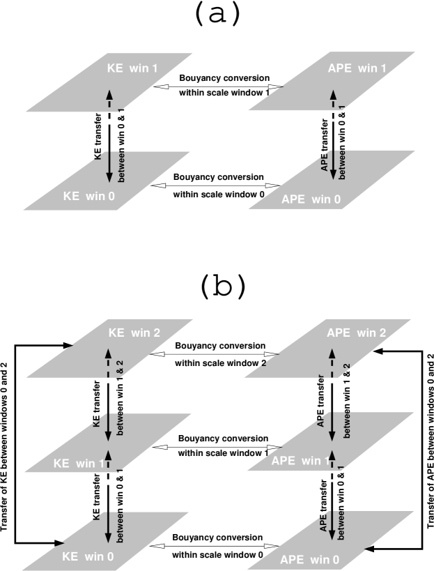
Figure 3: Schematic of the energy flow for (a) two-window decomposition, and (b) three-window decomposition. Clearly, buoyancy conversions take place within their respective scale windows; they are not indicators of instabilities. For clarity, the transfers $\Gamma^{0\oplus 2\to 1}$, $\Gamma^{1\oplus 2\to 0}$, $\Gamma^{0\oplus 1\to 2}$ are not drawn in (b). The transports of APE, KE, and pressure also take place within their respective scale windows only (not shown).

The energy flow for a multiple-scale window decomposition is schematized in Fig. 3. As is seen, canonical transfers mediate between the scale windows; they represent the interscale processes such as instabilities. In contrast, buoyancy conversions and transports function only within the respective individual windows; the former bring together the two types of energy, namely, APE and KE, while that latter allow different spatial locations to communicate.

V Multiscale oceanic energetics

V.1 Primitive equations

The multiscale ocean energy equations have been derived in LR05. We incorporate them here for completeness, together with some modification and correction.

For an incompressible and hydrostatic Boussinesq fluid flow, the primitive equations are:

$$\frac{\partial{\bf v}_{h}}{\partial t}+{\bf v}_{h}\cdot{\nabla_{h}}{\bf v}_{h}+w\frac{\partial{\bf v}_{h}}{\partial z}+f{\bf k}\times{\bf v}_{h}=-\frac{1}{\rho_{0}}{\nabla_{h}}P+{\bf F}_{m,z}+{\bf F}_{m,h}$$ (103)

$$\frac{\partial P}{\partial z}=-\rho g$$ (104)

$${\nabla_{h}}\cdot{\bf v}_{h}+\frac{\partial w}{\partial z}=0$$ (105)

$$\frac{\partial\rho}{\partial t}+{\bf v}_{h}\cdot{\nabla_{h}}\rho+w\frac{\partial\rho}{\partial z}=\frac{N^{2}\rho_{0}}{g}w+F_{\rho,z}+F_{\rho,h}$$ (106)

where the subgrid process parameterization are symbolically written as ${\bf F}_{m}$ and $F_{\rho}$. The other notations are referred to Appendix A.

V.2 Multiscale APE equation

Following Lorenz’ convention, available potential energy is defined to be

$$A=\frac{1}{2}\frac{g^{2}}{\rho_{0}^{2}N^{2}}\rho^{2}\equiv\frac{1}{2}c\rho^{2}$$ (107)

where

$$c=\frac{g^{2}}{\rho_{0}^{2}N^{2}}=\frac{g}{\rho_{0}s},\qquad{\rm and}\qquad s=-\frac{\partial\bar{\rho}(z)}{\partial z}.$$ (108)

A recent careful discussion on Boussinesq approximation and potential energy is referred to Ingersoll. As argued before, the multiscale APE on window $\varpi$ at step $n$ is $\frac{1}{2}c({\widehat{\rho}^{\sim\varpi}})^{2}.$ Take MWT on both sides of the equation of density anomaly, and multiply with $c{\widehat{\rho}^{\sim\varpi}}$. It has been shown by LR05 that, to a good approximation, $c{\widehat{\rho}^{\sim\varpi}}{\widehat{\left(\frac{\partial\rho}{\partial t}\right)}^{\sim\varpi}}$ can be identified as $\frac{\partial A_{n}^{\varpi}}{\partial t}$. The resulting APE equation is, therefore,

$$\frac{\partial A_{n}^{\varpi}}{\partial t}+c{\widehat{\rho}^{\sim\varpi}}{\widehat{\left({\bf v}\cdot{\nabla_{h}}\rho\right)}^{\sim\varpi}}+c{\widehat{\rho}^{\sim\varpi}}{\widehat{\left(w\frac{\partial\rho}{\partial z}\right)}^{\sim\varpi}}=\frac{g}{\rho_{0}}{\widehat{\rho}^{\sim\varpi}}{\widehat{w}^{\sim\varpi}}+F_{A,z}^{\varpi}+F_{A_{h}}^{\varpi},$$

where

$${\nabla_{h}}\rho=\frac{1}{a\cos\varphi}{\frac{\partial\rho}{\partial\lambda}}{\bf e}_{\lambda}+\frac{1}{a}{\frac{\partial\rho}{\partial\varphi}}{\bf e}_{\varphi},$$ (109)

and

$$\frac{g}{\rho_{0}}{\widehat{\rho}^{\sim\varpi}}{\widehat{w}^{\sim\varpi}}\equiv b_{n}^{\varpi}$$ (110)

is the rate of buoyancy conversion.

The key to the multiscale energetics formalism is the separation of flux and transfer processes. By that in subsection IIIIII.1, the flux of APE by ${\bf v}$ at step $n$ on window $\varpi$ is

$${\bf Q}_{A}^{\varpi}=\frac{1}{2}c{\widehat{\rho}^{\sim\varpi}}{\widehat{\left({\bf v}\rho\right)}^{\sim\varpi}}.$$ (111)

Hence the above equation can be written as

$$\frac{\partial A^{\varpi}}{\partial t}+{\nabla}\cdot{\bf Q}_{A}^{\varpi}=\left[-c{\widehat{\rho}^{\sim\varpi}}{\widehat{\left({\bf v}\cdot{\nabla}\rho\right)}^{\sim\varpi}}+{\nabla}\cdot{\bf Q}_{A}^{\varpi}\right]+b_{n}^{\varpi}+F_{A,z}^{\varpi}+F_{A,h}^{\varpi}.$$

But the bracket on the r.h.s. is still not the canonical transfer that we are seeking for. Since $c=c(z)$, it does not summarize to zero. In fact,

$$\sum_{\varpi}\sum_{n}\left[-c{\widehat{\rho}^{\sim\varpi}}{\widehat{\left({\bf v}\cdot{\nabla}\rho\right)}^{\sim\varpi}}+{\nabla}\cdot{\bf Q}_{A}^{\varpi}\right]=-c\overline{\rho{\nabla}\cdot(\rho{\bf v})}+\frac{1}{2}{\nabla}\cdot\left[c\overline{\rho({\bf v}\rho)}\right]$$

$$\qquad=\frac{1}{2}\frac{\partial c}{\partial z}\overline{\rho^{2}w},$$

where the overbar denotes averaging over the time period. Write

$$S_{A,n}^{\varpi}=\frac{1}{2}\frac{\partial c}{\partial z}{\widehat{\rho}^{\sim\varpi}}{\widehat{\left(\rho w\right)}^{\sim\varpi}}$$ (112)

which is the apparent source/sink due to the vertical stratification. Then

$$\Gamma_{A}^{\varpi} = \left[-c{\widehat{\rho}^{\sim\varpi}}{\widehat{\left({\bf v}\cdot{\nabla}\rho\right)}^{\sim\varpi}}+{\nabla}\cdot{\bf Q}_{A,n}^{\varpi}\right]-S_{A,n}^{\varpi}$$ (113)

$$= \frac{c}{2}\left[{\widehat{\left({\bf v}\rho\right)}^{\sim\varpi}}\cdot{\nabla}{\widehat{\rho}^{\sim\varpi}}-{\widehat{\rho}^{\sim\varpi}}{\nabla}\cdot{\widehat{\left({\bf v}\rho\right)}^{\sim\varpi}}\right]$$ (114)

proves to be canonical. The multiscale APE equation is, accordingly,

$$\frac{\partial A^{\varpi}}{\partial t}+{\nabla}\cdot{\bf Q}_{A}^{\varpi}=\Gamma_{A}^{\varpi}+b^{\varpi}+S_{A}^{\varpi}+F_{A,z}^{\varpi}+F_{A,h}^{\varpi}.$$ (115)

In the spherical coordinate frame, by (58), we have

$${\nabla}\cdot{\bf Q}_{A}^{\varpi} = \frac{c}{2a\cos\varphi}\left[{\frac{\partial\ }{\partial\lambda}}\left({\widehat{\rho}^{\sim\varpi}}{\widehat{\left(u\rho\right)}^{\sim\varpi}}\right)+{\frac{\partial\ }{\partial\varphi}}\left({\widehat{\rho}^{\sim\varpi}}{\widehat{\left(v\rho\right)}^{\sim\varpi}}\cos\varphi\right)\right]+\frac{1}{2}\frac{\partial\ }{\partial z}\left[c{\widehat{\rho}^{\sim\varpi}}{\widehat{\left(w\rho\right)}^{\sim\varpi}}\right],$$ (116)

and

$$\Gamma_{A}^{\varpi} =\frac{c}{2}\left[\frac{1}{a\cos\varphi}{\widehat{\left(u\rho\right)}^{\sim\varpi}}{\frac{\partial{\widehat{\rho}^{\sim\varpi}}}{\partial\lambda}}+\frac{1}{a}{\widehat{\left(v\rho\right)}^{\sim\varpi}}{\frac{\partial{\widehat{\rho}^{\sim\varpi}}}{\partial\varphi}}+{\widehat{\left(w\rho\right)}^{\sim\varpi}}\frac{\partial{\widehat{\rho}^{\sim\varpi}}}{\partial z}\right.$$ (118)

$$\ \ \left.-{\widehat{\rho}^{\sim\varpi}}\left(\frac{1}{a\cos\varphi}{\frac{\partial{\widehat{\left(u\rho\right)}^{\sim\varpi}}}{\partial\lambda}}+\frac{1}{a\cos\varphi}{\frac{\partial{\widehat{\left(v\rho\right)}^{\sim\varpi}}\cos\varphi}{\partial\varphi}}+\frac{\partial{\widehat{\left(w\rho\right)}^{\sim\varpi}}}{\partial z}\right)\right]$$

V.3 The KE equation

The equation governing the evolution of the multiscale kinetic energy (KE)

$$K^{\varpi}=\frac{1}{2}{\widehat{{\bf v}}^{\sim\varpi}}\cdot{\widehat{{\bf v}}^{\sim\varpi}}$$ (119)

can be obtained by taking MWT on both sides of the horizontal momentum equations, followed by a dot product with ${\widehat{{\bf v}}^{\sim\varpi}}$. This results in

$$\frac{\partial K_{n}^{\varpi}}{\partial t}+{\widehat{\left({\bf v}\cdot{\nabla}{\bf v}_{h}\right)}^{\sim\varpi}}\cdot{\widehat{{\bf v}}_{h}^{\sim\varpi}}=-\frac{1}{\rho_{0}}{\bf v}_{h}\cdot{\nabla_{h}}{\widehat{P}^{\sim\varpi}}+F_{K,z}^{\varpi}+F_{K,h}^{\varpi}$$

$$=-{\bf v}\cdot{\nabla}\frac{{\widehat{P}^{\sim\varpi}}}{\rho_{0}}+{\widehat{w}^{\sim\varpi}}\frac{\partial{\widehat{P}^{\sim\varpi}}/\rho_{0}}{\partial z}+F_{K,z}^{\varpi}+F_{K,h}^{\varpi}$$

$$=-{\nabla}\cdot\left({\widehat{{\bf v}}^{\sim\varpi}}\frac{{\widehat{P}^{\sim\varpi}}}{\rho_{0}}\right)-\frac{g}{\rho_{0}}{\widehat{\rho}^{\sim\varpi}}{\widehat{w}^{\sim\varpi}}+F_{K,z}^{\varpi}+F_{K,h}^{\varpi}$$

$$\equiv-{\nabla}\cdot{\bf Q}_{P}^{\varpi}-b^{\varpi}+F_{K,z}^{\varpi}+F_{K,h}^{\varpi},$$

where $b^{\varpi}$ is the buoyancy conversion rate, and $-{\nabla}\cdot{\bf Q}_{P}^{\varpi}$ the pressure working rate. In the above derivation Eqs. (104) and (105) (incompressibility and hydrostaticity) have been used.

By the transport-transfer separation, the above multiscale KE equation can be written as

$$\frac{\partial K^{\varpi}}{\partial t}+{\nabla}\cdot{\bf Q}_{K}^{\varpi}=\Gamma_{K}^{\varpi}-{\nabla}\cdot{\bf Q}_{P}^{\varpi}-b^{\varpi}+F_{K,z}^{\varpi}+F_{K,h}^{\varpi},$$ (120)

where

$${\bf Q}_{K}^{\varpi}=\frac{1}{2}{\widehat{\left({\bf v}{\bf v}_{h}\right)}^{\sim\varpi}}\cdot{\widehat{{\bf v}}_{h}^{\sim\varpi}},$$ (121)

and

$$\Gamma_{K}^{\varpi} = -{\widehat{\left({\bf v}\cdot{\nabla}{\bf v}_{h}\right)}^{\sim\varpi}}\cdot{\widehat{{\bf v}}_{h}^{\sim\varpi}}+{\nabla}\cdot{\bf Q}_{K}^{\varpi}$$ (122)

$$= -{\nabla}\cdot{\widehat{\left({\bf v}{\bf v}_{h}\right)}^{\sim\varpi}}\cdot{\widehat{{\bf v}}_{h}^{\sim\varpi}}+{\nabla}\cdot{\bf Q}_{K,n}^{\varpi}$$ (123)

$$= \frac{1}{2}\left[{\widehat{\left({\bf v}{\bf v}_{h}\right)}^{\sim\varpi}}:{\nabla}{\widehat{{\bf v}}_{h}^{\sim\varpi}}-[{\nabla}\cdot{\widehat{\left({\bf v}{\bf v}_{h}\right)}^{\sim\varpi}}]\cdot{\widehat{{\bf v}}_{h}^{\sim\varpi}}\right],$$ (124)

which are precisely the same as that for the atmosphere case. In the spherical coordinates $(\lambda,\varphi,z)$, ${\nabla}\cdot{\bf Q}_{K}^{\varpi}$ and $\Gamma_{K}^{\varpi}$ are also like that in (60) and (81), except that $\omega$ should be replaced by $w$, and $p$ by $z$.

V.3.1 Wrap-up

To wrap up, the multiscale ocean energetic equations are

$$\frac{\partial A^{\varpi}}{\partial t}+{\nabla}\cdot Q_{A}^{\varpi}=\Gamma_{A}^{\varpi}+b^{\varpi}+S_{A}^{\varpi}+F_{A,z}^{\varpi}+F_{A,h}^{\varpi},$$ (125)

$$\frac{\partial K^{\varpi}}{\partial t}+{\nabla}\cdot Q_{K}^{\varpi}=\Gamma_{K^{\varpi}}-{\nabla}\cdot{\bf Q}_{P}^{\varpi}-b^{\varpi}+F_{K,z}^{\varpi}+F_{K,h}^{\varpi}.$$ (126)

The expressions are referred to Table 3.

Table 3: Multiscale energetics for oceanic circulations. The expressions in spherical coordinates are the same in form as that in Table 2, except that the coordinate $p$ should be replaced by $z$ and $T$ by $\rho$. The units are in $m^{2}s^{-3}$ (if SI units are used). All terms are to be multiplied by $2^{j_{2}}$.

$K^{\varpi}$	$\frac{1}{2}{\widehat{{\bf v}}_{h}^{\sim\varpi}}\cdot{\widehat{{\bf v}}_{h}^{\sim\varpi}}$	KE on scale window $\varpi$
${\bf Q}_{K}^{\varpi}$	$\frac{1}{2}[{\widehat{\left({\bf v}{\bf v}_{h}\right)}^{\sim\varpi}}\cdot{\widehat{{\bf v}}_{h}^{\sim\varpi}}]$	flux of KE on window $\varpi$
$\Gamma_{K}^{\varpi}$	$\frac{1}{2}[{\widehat{\left({\bf v}{\bf v}_{h}\right)}^{\sim\varpi}}:{\nabla}{\widehat{{\bf v}}_{h}^{\sim\varpi}}-{\nabla}\cdot{\widehat{\left({\bf v}{\bf v}_{h}\right)}^{\sim\varpi}}\cdot{\widehat{{\bf v}}_{h}^{\sim\varpi}}]$	canonical transfer of KE to window $\varpi$
${\bf Q}_{P}^{\varpi}$	${\frac{1}{\rho_{0}}{\widehat{{\bf v}}^{\sim\varpi}}{\widehat{P}^{\sim\varpi}}}$	pressure flux on window $\varpi$
$b^{\varpi}$	$\frac{g}{\rho_{0}}{\widehat{\rho}^{\sim\varpi}}{\widehat{w}^{\sim\varpi}}$	buoyancy conversion on window $\varpi$
$A^{\varpi}$	$\frac{1}{2}c({\widehat{\rho}^{\sim\varpi}})^{2}$,   $c=\frac{g^{2}}{\rho_{0}^{2}N^{2}}$	APE on window $\varpi$
${\bf Q}_{A}^{\varpi}$	$\frac{1}{2}[c{\widehat{\rho}^{\sim\varpi}}{\widehat{\left({\bf v}\rho\right)}^{\sim\varpi}}]$	flux of APE on window $\varpi$
$\Gamma_{A}^{\varpi}$	$\frac{c}{2}[{\widehat{\left({\bf v}\rho\right)}^{\sim\varpi}}\cdot{\nabla}{\widehat{\rho}^{\sim\varpi}}-{\widehat{\rho}^{\sim\varpi}}{\nabla}\cdot{\widehat{\left({\bf v}\rho\right)}^{\sim\varpi}}]$	canonical transfer of APE to window $\varpi$
$S_{A}^{\varpi}$	$\frac{1}{2}{\widehat{\rho}^{\sim\varpi}}{\widehat{\left(\omega\rho\right)}^{\sim\varpi}}\frac{\partial c}{\partial z}$	apparent source/sink of $A^{\varpi}$ (usually negligible)

VI Multiscale quasi-geostrophic energetics

The multiscale energy equations like (57) and (97) cannot be directly derived from the quasi-geostrophic (QG) equation. We have to go back to where the QG equation comes from and do the derivation, and this is how Pinardi did with their regional QG energetics.

Since the atmospheres and oceans share the same QG equation, it suffices to start off the derivation from either (43)-(47) or (103)-(106). As vertically a $z$ coordinate is desired, we choose the latter. To simplify the presentation, the dissipative and diffusive processes are omitted. They are not essential to the derivation, and their effect may be added symbolically after the other terms are finalized. From Appendix C, the QG equation we will be dealing with is:

$$\frac{\partial\ }{\partial t}\left[{\nabla_{h}}^{2}\psi+\frac{\partial\ }{\partial z}\left(\frac{{F_{r}}^{2}}{N^{2}}\frac{\partial\psi}{\partial z}\right)\right]+{\alpha_{\ell}}J\left(\psi,\ \left[{\nabla_{h}}^{2}\psi+\frac{\partial\ }{\partial z}\left(\frac{{F_{r}}^{2}}{N^{2}}\frac{\partial\psi}{\partial z}\right)\right]\right)+\beta\frac{\partial\psi}{\partial x}=0,$$ (127)

where ${F_{r}}$ is the rotational internal Froude number, ${\alpha_{\ell}}$ a dimensionless measure of the importance of advection, and $J$ the Jacobian operator; the other notations are conventional and referred to Appendix A.

VI.1 QG kinetic energetics

The inviscid version of the KE equation (125) is rewritten as

$$\frac{\partial K^{\varpi}}{\partial t}+{\nabla_{h}}\cdot{{\bf Q}}_{K,h}^{\varpi}+\frac{\partial Q_{K,z}^{\varpi}}{\partial z}=\Gamma_{K,h}^{\varpi}+\Gamma_{K,z}^{\varpi}-{\nabla_{h}}\cdot{{\bf Q}}_{P,h}^{\varpi}-\frac{\partial Q_{P,z}^{\varpi}}{\partial z}-b^{\varpi},$$ (128)

where

$$\Gamma_{K,h}^{\varpi}=-{\nabla_{h}}\cdot{\widehat{\left({\bf v}_{h}{\bf v}_{h}\right)}^{\sim\varpi}}\cdot{\widehat{{\bf v}}_{h}^{\sim\varpi}}+{\nabla_{h}}\cdot{\bf Q}_{K,h}^{\varpi},$$ (129)

$$\Gamma_{K,z}^{\varpi}=-\frac{\partial{\widehat{\left(w{\bf v}_{h}\right)}^{\sim\varpi}}}{\partial z}\cdot{\widehat{{\bf v}}_{h}^{\sim\varpi}}+\frac{\partial Q_{K,z}^{\varpi}}{\partial z}.$$ (130)

In the transport and transfer terms, the effects due to the horizontal and vertical advections are distinguished. As we will see soon, this will greatly help simplify the QG energetics.

Using the usual scaling (e.g., McWilliams_book ),

$$(x,y)\sim L_{0},\qquad z\sim H_{0},\qquad t\sim t_{0},$$

$$(u,v)\sim U_{0},\qquad w\sim\frac{H_{0}}{L_{0}}U_{0},$$

$$f\sim f_{0},\qquad N\sim N_{0},$$

$$P\sim U_{0}f_{0}\rho_{0}L_{0},\qquad\rho\sim\frac{f_{0}U_{0}L_{0}}{gH_{0}}\rho_{0},$$

and noticing that the multiscale window transform does not affect the scaling, it is easy to have

$$\frac{\partial K^{\varpi}}{\partial t}\sim\frac{U_{0}^{2}}{t_{0}};$$

$${\nabla_{h}}{\bf Q}_{K,h}^{\varpi}\ {\rm and}\ \frac{\partial Q_{K,z}^{\varpi}}{\partial z}\ \sim\ \frac{U_{0}^{3}}{L_{0}};$$

$$\Gamma_{K,h}^{\varpi}\ {\rm and}\ \Gamma_{K,z}^{\varpi}\ \sim\ \frac{U_{0}^{3}}{L_{0}};$$

$${\nabla_{h}}\cdot{\bf Q}_{P,h}^{\varpi}\ {\rm and}\ \frac{\partial Q_{P,z}^{\varpi}}{\partial z}\ \sim U_{0}^{2}f_{0};$$

$$b^{\varpi}=\frac{g}{\rho_{0}}{\widehat{\rho}^{\sim\varpi}}{\widehat{w}^{\sim\varpi}}\sim U_{0}^{2}f_{0}.$$

This will yield the nondimensionalized kinetic energetics.

For clarity, hereafter throughout this subsection, all variables are understood as nondimensional. From above, Eq. (128) is now reduced to its nondimensional form:

$${\varepsilon}\frac{\partial K^{\varpi}}{\partial t}+{\varepsilon}{\alpha_{\ell}}{\nabla_{h}}\cdot{{\bf Q}}_{K,h}^{\varpi}+{\varepsilon}{\alpha_{\ell}}\frac{\partial Q_{K,h}^{\varpi}}{\partial z}={\varepsilon}{\alpha_{\ell}}\Gamma_{K,h}^{\varpi}+{\varepsilon}{\alpha_{\ell}}\Gamma_{K,z}^{\varpi}-{\nabla_{h}}\cdot{{\bf Q}}_{P,h}^{\varpi}-\frac{\partial Q_{P,z}^{\varpi}}{\partial z}-b^{\varpi},$$ (131)

where ${\varepsilon}=\frac{1}{f_{0}t_{0}}$ is the Rossby number, ${\alpha_{\ell}}=\frac{U_{0}t_{0}}{L_{0}}$ measures the relative importance of advection to local change. In many textbooks, ${\alpha_{\ell}}$ is taken to be one, so that ${\varepsilon}{\alpha_{\ell}}=U_{0}/f_{0}L_{0}$ is defined as the Rossby number.

As usual, expand the variables in the power of ${\varepsilon}$,

$$P=[P]_{0}+{\varepsilon}[P]_{1}+{\varepsilon}^{2}[P]_{2}...$$ (132)

$$w=[w]_{0}+{\varepsilon}[w]_{1}+{\varepsilon}^{2}[w]_{2}...$$ (133)

$${\bf v}_{h}=[{\bf v}_{h}]_{0}+{\varepsilon}[{\bf v}_{h}]_{1}+{\varepsilon}^{2}[{\bf v}_{h}]_{2}...$$ (134)

$$\rho=[\rho]_{0}+{\varepsilon}[\rho]_{1}+{\varepsilon}^{2}[\rho]_{2}...$$ (135)

Based on these expansions the multiscale energetic terms can also be expanded. For example,

$$K=[K]_{0}+{\varepsilon}[K]_{1}+\ldots$$

where $[K]_{0}=\frac{1}{2}[{\bf v}_{h}]_{0}\cdot[{\bf v}_{h}]_{0}$, $[K]_{1}=[{\bf v}_{h}]_{0}\cdot[{\bf v}_{h}]_{1}$, and so forth. By the classical result [see (199)-(201) in App. C], $[w]_{0}=0$. So

$${\varepsilon}\frac{\partial Q_{K,z}^{\varpi}}{\partial z}={\varepsilon}\frac{\partial\ }{\partial z}\frac{1}{2}\left\{{\widehat{\left(w{\bf v}_{h}\right)}^{\sim\varpi}}\cdot{{\bf v}_{h}}\right\}\ \sim\ O({\varepsilon}^{2}).$$

Likewise,

$${\varepsilon}\Gamma_{K,z}^{\varpi}\sim O({\varepsilon}^{2}),$$

$$\frac{\partial\ }{\partial z}Q_{P,z}^{\varpi}=\frac{\partial\ }{\partial z}({\widehat{w}^{\sim\varpi}}{\widehat{P}^{\sim\varpi}})={\varepsilon}\frac{\partial\ }{\partial z}([{\widehat{w}^{\sim\varpi}}]_{1}[{\widehat{P}^{\sim\varpi}}]_{0})+O({\varepsilon}^{2}),$$

$$b^{\varpi}={\widehat{\rho}^{\sim\varpi}}{\widehat{w}^{\sim\varpi}}={\varepsilon}[{\widehat{\rho}^{\sim\varpi}}]_{0}[{\widehat{w}^{\sim\varpi}}]_{1}+O({\varepsilon}^{2}).$$

Substituting the power expansions into (131), taking into account the above facts, and equating the terms of like power, we have, to the order of $O({\varepsilon}^{0})$,

$$\qquad{\nabla_{h}}\cdot\left([{\widehat{{\bf v}}_{h}^{\sim\varpi}}]_{0}[{\widehat{P}^{\sim\varpi}}]_{0}\right)=0.$$

So a huge part of the pressure working rate is actually zero. To the order of $O({\varepsilon}^{1})$,

$$\frac{\partial[K^{\varpi}]_{0}}{\partial t}+{\alpha_{\ell}}{\nabla_{h}}\cdot[{\bf Q}_{K,h}^{\varpi}]_{0}={\alpha_{\ell}}[\Gamma_{K,h}^{\varpi}]_{0}-{\nabla_{h}}\cdot[{\bf Q}_{P,h}^{\varpi}]_{1}-\frac{\partial\ }{\partial z}[Q_{P,z}^{\varpi}]_{1}-[b^{\varpi}]_{1}$$

$$={\alpha_{\ell}}\Gamma_{K,h}^{\varpi}-{\nabla_{h}}\cdot\left([{\widehat{{\bf v}}_{h}^{\sim\varpi}}]_{0}[{\widehat{P}^{\sim\varpi}}]_{1}+[{\widehat{{\bf v}}_{h}^{\sim\varpi}}]_{1}[{\widehat{P}^{\sim\varpi}}]_{0}\right)-\frac{\partial\ }{\partial z}\left([{\widehat{w}^{\sim\varpi}}]_{1}[{\widehat{P}^{\sim\varpi}}]_{0}\right)-[{\widehat{\rho}^{\sim\varpi}}]_{0}[{\widehat{w}^{\sim\varpi}}]_{1}.$$

To this order, $[{\bf v}_{h}]_{0}$ is the geostrophic flow: $[{\bf v}_{h}]_{0}={\bf k}\times{\nabla}[P]_{0}$, $[\rho]_{0}$ is $-\frac{\partial\ }{\partial z}[P]_{0}$ by hydrostaticity. $[w]_{1}$ and $[{\bf v}_{h}]_{1}$ can also be obtained [see (202)-(203) in App. C]:

$$[w]_{1}=-\frac{{F_{r}}^{2}}{N^{2}}{\mathscr{L}}\left(\frac{\partial[P]_{0}}{\partial z}\right),$$

$$[{\bf v}_{h}]_{1}={\bf k}\times{\mathscr{L}}([{\bf v}_{h}]_{0})-\beta y[{\bf v}_{h}]_{0}+{\bf k}\times{\nabla_{h}}[P]_{1},$$

where ${F_{r}}=\frac{f_{0}L_{0}}{N_{0}H_{0}}$ is the rotational internal Froude number, and $\mathscr{L}$ stands for the operator

$${\mathscr{L}}\equiv\frac{\partial\ }{\partial t}+{\alpha_{\ell}}[{\bf v}_{h}]_{0}\cdot{\nabla_{h}}$$ (136)

(advection by the geostrophic flow). With these, it is straightforward to compute $[K^{\varpi}]_{0}$, $[{\bf Q}_{K,h}^{\varpi}]_{0}$, $[\Gamma_{K,h}^{\varpi}]_{0}$, $\frac{\partial\ }{\partial z}[Q_{P,z}^{\varpi}]_{1}$ and $[b^{\varpi}]_{1}$. The difficulty comes from the horizontal pressure working rate $[{\bf Q}_{P,h}^{\varpi}]_{1}$, where $[{\widehat{P}^{\sim\varpi}}]_{1}$ is involved. But

$${\nabla_{h}}\cdot\left([{\widehat{{\bf v}}_{h}^{\sim\varpi}}]_{0}[{\widehat{P}^{\sim\varpi}}]_{1}+[{\widehat{{\bf v}}_{h}^{\sim\varpi}}]_{1}[{\widehat{P}^{\sim\varpi}}]_{0}\right)$$

$$={\nabla_{h}}\cdot\left([{\widehat{{\bf v}}_{h}^{\sim\varpi}}]_{0}[{\widehat{P}^{\sim\varpi}}]_{1}+({\bf k}\times{\widehat{\left({\mathscr{L}}[{\bf v}_{h}]_{0}\right)}^{\sim\varpi}}-\beta y[{\widehat{{\bf v}}_{h}^{\sim\varpi}}]_{0}+{\bf k}\times{\nabla_{h}}[{\widehat{P}^{\sim\varpi}}]_{1})[{\widehat{P}^{\sim\varpi}}]_{0}\right)$$

$$={\nabla_{h}}\cdot(({\bf k}\times{\widehat{\left({\mathscr{L}}[{\bf v}_{h}]_{0}\right)}^{\sim\varpi}}-\beta y[{\widehat{{\bf v}}_{h}^{\sim\varpi}}]_{0})[{\widehat{P}^{\sim\varpi}}]_{0})+{\nabla_{h}}\cdot([{\widehat{{\bf v}}_{h}^{\sim\varpi}}]_{0}[{\widehat{P}^{\sim\varpi}}]_{1}+{\bf k}\times{\nabla_{h}}[{\widehat{P}^{\sim\varpi}}]_{1}[{\widehat{P}^{\sim\varpi}}]_{0}).$$

Notice that the second divergence vanishes. In fact, it is

$${\nabla_{h}}\cdot({\bf k}\times{\nabla_{h}}[{\widehat{P}^{\sim\varpi}}]_{0}[{\widehat{P}^{\sim\varpi}}]_{1}+{\bf k}\times{\nabla_{h}}[{\widehat{P}^{\sim\varpi}}]_{1}[{\widehat{P}^{\sim\varpi}}]_{0})$$

$$=-{\bf k}\cdot{\nabla_{h}}\times({\nabla_{h}}[{\widehat{P}^{\sim\varpi}}]_{0}[{\widehat{P}^{\sim\varpi}}]_{1}+{\nabla_{h}}[{\widehat{P}^{\sim\varpi}}]_{1}[{\widehat{P}^{\sim\varpi}}]_{0})$$

$$=0.$$

Hence the whole pressure working rate

$${\nabla_{h}}\cdot[{\bf Q}_{P,h}^{\varpi}]_{1}={\nabla_{h}}\cdot(({\bf k}\times{\widehat{\left({\mathscr{L}}[{\bf v}_{h}]_{0}\right)}^{\sim\varpi}}-\beta y[{\widehat{{\bf v}}_{h}^{\sim\varpi}}]_{0})[{\widehat{P}^{\sim\varpi}}]_{0}).$$ (137)

As a convention, denote $[P]_{0}$ as $\psi$, and for convenience, write $[{\bf v}_{h}]_{0}={\bf k}\times{\nabla_{h}}\psi$ as ${\bf v}_{g}$ (geostrophic velocity). Distinguishing the QG energetics terms with a subscript $g$, the multiscale KE now becomes

$$\frac{\partial\ }{\partial t}K_{g}^{\varpi}+{\nabla_{h}}\cdot{\bf Q}_{K,g}^{\varpi}=\Gamma_{K,g}^{\varpi}-{\nabla_{h}}\cdot{\bf Q}_{P,g,h}^{\varpi}-\frac{\partial\ }{\partial z}Q_{P,g,z}^{\varpi}-b_{g}^{\varpi},$$ (138)

where

$$K_{g}^{\varpi}=\frac{1}{2}{\widehat{{\bf v}_{g}}^{\sim\varpi}}\cdot{\widehat{{\bf v}_{g}}^{\sim\varpi}},$$ (139)

$$Q_{K,g}^{\varpi}={\alpha_{\ell}}{\bf[}Q_{K,h}^{\varpi}]_{0}=\frac{1}{2}{\alpha_{\ell}}{\widehat{\left({\bf v}_{g}{\bf v}_{g}\right)}^{\sim\varpi}}\cdot{\widehat{{\bf v}_{g}}^{\sim\varpi}},$$ (140)

$$\Gamma_{K,g}^{\varpi}={\alpha_{\ell}}[\Gamma_{K,h}^{\varpi}]_{0}=\frac{{\alpha_{\ell}}}{2}\left[{\widehat{\left({\bf v}_{g}{\bf v}_{g}\right)}^{\sim\varpi}}:{\nabla_{h}}{\widehat{{\bf v}_{g}}^{\sim\varpi}}-{\nabla_{h}}\cdot{\widehat{\left({\bf v}_{g}{\bf v}_{g}\right)}^{\sim\varpi}}\cdot{\widehat{{\bf v}_{g}}^{\sim\varpi}}\right]$$ (141)

$${\bf Q}_{P,g,h}^{\varpi}=({\bf k}\times{\mathscr{L}}({\widehat{{\bf v}_{g}}^{\sim\varpi}})-\beta y{\widehat{{\bf v}_{g}}^{\sim\varpi}}){\widehat{\psi}^{\sim\varpi}}$$ (142)

$$Q_{P,g,z}^{\varpi}=-\frac{{F_{r}}^{2}}{N^{2}}{\widehat{\psi}^{\sim\varpi}}{\widehat{\left({\mathscr{L}}\left(\frac{\partial\psi}{\partial z}\right)\right)}^{\sim\varpi}}$$ (143)

$$b_{g}^{\varpi}=\frac{{F_{r}}^{2}}{N^{2}}\frac{\partial{\widehat{\psi}^{\sim\varpi}}}{\partial z}{\widehat{\left({\mathscr{L}}\left(\frac{\partial\psi}{\partial z}\right)\right)}^{\sim\varpi}}$$ (144)

(recall that all are to be multiplied by a constant fact $2^{j_{2}}$).

VI.2 QG available potential energetics

Rewrite the nondiffusive version of the APE equation (126) as

$$\frac{\partial A^{\varpi}}{\partial t}+{\nabla_{h}}\cdot{{\bf Q}}_{A,h}^{\varpi}+\frac{\partial Q_{A,z}^{\varpi}}{\partial z}=\Gamma_{A,h}^{\varpi}+\Gamma_{A,z}^{\varpi}+b^{\varpi}+S_{A}^{\varpi}.$$ (145)

Using the scaling as shown in the preceding subsection, we have

$$\frac{\partial A^{\varpi}}{\partial t}=\frac{1}{2}\frac{g^{2}}{\rho_{0}^{2}N^{2}}\left({\widehat{\rho}^{\sim\varpi}}\right)^{2}\sim\frac{1}{t_{0}}\frac{g^{2}}{\rho_{0}^{2}N_{0}^{2}}\left(\frac{f_{0}U_{0}L_{0}}{gH_{0}}\rho_{0}\right)^{2}$$

$$\qquad=\frac{U_{0}^{2}}{t_{0}}\frac{f_{0}^{2}L_{0}^{2}}{N_{0}^{2}H_{0}^{2}}\equiv\frac{U_{0}^{2}}{t_{0}}{F_{r}}^{2}$$

$${\nabla_{h}}\cdot{\bf Q}_{A,h}^{\varpi}\sim\frac{1}{L_{0}}\frac{g^{2}}{\rho_{0}^{2}N_{0}^{2}}U_{0}\left(\frac{f_{0}U_{0}L_{0}}{gH_{0}}\rho_{0}\right)^{2}=\frac{U_{0}^{3}}{L_{0}}{F_{r}}^{2},$$

where ${F_{r}}=\frac{f_{0}L_{0}}{N_{0}H_{0}}$ is the rotational internal Froude number (compared to the Froude number $\frac{U_{0}}{N_{0}H_{0}}$). Likewise, all the remaining terms, except $b^{\varpi}\sim U_{0}^{2}f_{0}$ (as given in the preceding subsection), are of the order of $\frac{U_{0}^{3}}{L_{0}}{F_{r}}^{2}$.

As in the preceding subsection, let ${\varepsilon}=\frac{1}{f_{0}t_{0}}$ be the Rossby number and let ${\alpha_{\ell}}=\frac{U_{0}t_{)}}{L_{0}}$. The scaled nondiffusive APE equation (from now on throughout this subsection all the variables are nondimensional) is, therefore,

$${\varepsilon}{F_{r}}^{2}\left(\frac{\partial A^{\varpi}}{\partial t}+{\alpha_{\ell}}{\nabla_{h}}\cdot{\bf Q}_{A,h}^{\varpi}+{\alpha_{\ell}}\frac{\partial\ }{\partial z}Q_{A,z}^{\varpi}\right)={\varepsilon}{F_{r}}^{2}{\alpha_{\ell}}(\Gamma_{A,h}^{\varpi}+\Gamma_{A,z}^{\varpi})+b^{\varpi}+{\varepsilon}{F_{r}}^{2}S_{A}^{\varpi}.$$ (146)

Usually ${F_{r}}$ is taken as order of $O(1)$, but ${\varepsilon}$ is small. Expanding in the power of ${\varepsilon}$, since $[w]_{0}=0$ (cf. App. C), it is easy to show that

$${\varepsilon}\frac{\partial\ }{\partial z}Q_{A,z}^{\varpi}\sim{\varepsilon}\Gamma_{A,z}^{\varpi}\sim{\varepsilon}S_{A}^{\varpi}\ \sim\ O({\varepsilon}^{2}).$$

In other words, when only order of $O({\varepsilon})$ is considered, all these terms are negligible. Therefore, the resulting APE equation is, to the order of $O({\varepsilon})$,

$${F_{r}}^{2}\frac{\partial[A^{\varpi}]_{0}}{\partial t}+{\alpha_{\ell}}{F_{r}}^{2}{\nabla_{h}}\cdot[{\bf Q}_{A,h}^{\varpi}]_{0}={\alpha_{\ell}}{F_{r}}^{2}[\Gamma_{A,h}^{\varpi}]_{0}+[b^{\varpi}]_{1}.$$ (147)

For clarity, this is symbolically written as

$$\frac{\partial\ }{\partial t}A_{g}^{\varpi}+{\nabla_{h}}\cdot{\bf Q}_{g,A}^{\varpi}=\Gamma_{g,A}^{\varpi}+b_{g}^{\varpi},$$ (148)

where

$$A_{g}^{\varpi}={F_{r}}^{2}[A^{\varpi}]_{0}=\frac{{F_{r}}^{2}}{2}\frac{1}{N^{2}}\left(\frac{\partial{\widehat{\Psi}^{\sim\varpi}}}{\partial z}\right)^{2}$$

$${\bf Q}_{g,A}^{\varpi}={\alpha_{\ell}}{F_{r}}^{2}[{\bf Q}_{A,h}^{\varpi}]_{0}=\frac{{\alpha_{\ell}}}{2}\frac{{F_{r}}^{2}}{Nr}\frac{\partial{\widehat{\Psi}^{\sim\varpi}}}{\partial z}{\widehat{\left({\bf v}_{g}\frac{\partial\Psi}{\partial z}\right)}^{\sim\varpi}}$$

$$\Gamma_{g,A}^{\varpi}={\alpha_{\ell}}{F_{r}}^{2}[\Gamma_{A,h}^{\varpi}]_{0}=\frac{{\alpha_{\ell}}}{2}\frac{{F_{r}}^{2}}{N^{2}}\left[{\widehat{\left({\bf v}_{g}\frac{\partial\Psi}{\partial z}\right)}^{\sim\varpi}}\cdot{\nabla_{h}}\frac{\partial{\widehat{\Psi}^{\sim\varpi}}}{\partial z}-\frac{\partial{\widehat{\Psi}^{\sim\varpi}}}{\partial z}{\nabla_{h}}\cdot{\widehat{\left({\bf v}_{g}\frac{\partial\Psi}{\partial z}\right)}^{\sim\varpi}}\right]$$

$$b_{g}^{\varpi}=[b^{\varpi}]_{1}=\frac{{F_{r}}^{2}}{N^{2}}\frac{\partial{\widehat{\psi}^{\sim\varpi}}}{\partial z}{\widehat{\left({\mathscr{L}}\left(\frac{\partial\psi}{\partial z}\right)\right)}^{\sim\varpi}}$$

VI.3 Wrap-up

To summarize, the multiscale energy equations for the inviscid QG equation (127) are

$$\frac{\partial\ }{\partial t}A_{g}^{\varpi}+{\nabla_{h}}\cdot{\bf Q}_{g,A}^{\varpi}=\Gamma_{g,A}^{\varpi}+b_{g}^{\varpi},$$ (149)

$$\frac{\partial\ }{\partial t}K_{g}^{\varpi}+{\nabla_{h}}\cdot{\bf Q}_{g,K}^{\varpi}=\Gamma_{g,K}^{\varpi}-{\nabla_{h}}\cdot{\bf Q}_{g,P,h}^{\varpi}-\frac{\partial\ }{\partial z}Q_{g,P,z}^{\varpi}-b_{g}^{\varpi}.$$ (150)

The explicit expressions of the energetic terms are tabulated in Table 4.

Table 4: Expansion of the QG energetics for Eq. (127). ${\bf v}_{g}={\bf k}\times{\nabla_{h}}\psi$, ${\mathscr{L}}=\frac{\partial\ }{\partial t}+J(\psi,.)$.

$K_{g}^{\varpi}$	$\frac{1}{2}{\widehat{{\bf v}_{g}}^{\sim\varpi}}\cdot{\widehat{{\bf v}_{g}}^{\sim\varpi}}$	QG KE on scale window $\varpi$
$Q_{K,g}^{\varpi}$	$\frac{1}{2}{\alpha_{\ell}}{\widehat{\left({\bf v}_{g}{\bf v}_{g}\right)}^{\sim\varpi}}\cdot{\widehat{{\bf v}_{g}}^{\sim\varpi}}$	Flux of QG KE within scale window $\varpi$
$\Gamma_{K,g}^{\varpi}$	$\frac{{\alpha_{\ell}}}{2}\left[{\widehat{\left({\bf v}_{g}{\bf v}_{g}\right)}^{\sim\varpi}}:{\nabla_{h}}{\widehat{{\bf v}_{g}}^{\sim\varpi}}-{\nabla_{h}}\cdot{\widehat{\left({\bf v}_{g}{\bf v}_{g}\right)}^{\sim\varpi}}\cdot{\widehat{{\bf v}_{g}}^{\sim\varpi}}\right]$	canonical transfer of QG KE to window $\varpi$
${\bf Q}_{P,g,h}^{\varpi}$	$[{\bf k}\times{\widehat{\left({\mathscr{L}}({\bf v}_{g})\right)}^{\sim\varpi}}-\beta y{\widehat{{\bf v}_{g}}^{\sim\varpi}}]{\widehat{\psi}^{\sim\varpi}}$	horizontal pressure flux on window $\varpi$
$Q_{P,g,z}^{\varpi}$	$-\frac{{F_{r}}^{2}}{N^{2}}{\widehat{\psi}^{\sim\varpi}}\left[\frac{\partial^{2}{\widehat{\psi}^{\sim\varpi}}}{\partial t\partial z}+{\alpha_{\ell}}{\widehat{\left({\bf v}_{g}\cdot{\nabla_{h}}\frac{\partial\psi}{\partial z}\right)}^{\sim\varpi}}\right]$	vertical pressure flux on window $\varpi$
$b_{g}^{\varpi}$	$\frac{{F_{r}}^{2}}{N^{2}}\frac{\partial{\widehat{\psi}^{\sim\varpi}}}{\partial z}{\widehat{\left({\mathscr{L}}\left(\frac{\partial\psi}{\partial z}\right)\right)}^{\sim\varpi}}$	rate of buoyancy conversion on window $\varpi$
$A_{g}^{\varpi}$	$\frac{{F_{r}}^{2}}{2}\frac{1}{N^{2}}\left(\frac{\partial{\widehat{\Psi}^{\sim\varpi}}}{\partial z}\right)^{2}$	QG APE on scale window $\varpi$
${\bf Q}_{A,g}^{\varpi}$	$\frac{{\alpha_{\ell}}}{2}\frac{{F_{r}}^{2}}{Nr}\frac{\partial{\widehat{\Psi}^{\sim\varpi}}}{\partial z}{\widehat{\left({\bf v}_{g}\frac{\partial\Psi}{\partial z}\right)}^{\sim\varpi}}$	flux of QG APE within window $\varpi$
$\Gamma_{A,g}^{\varpi}$	$\frac{{\alpha_{\ell}}}{2}\frac{{F_{r}}^{2}}{N^{2}}\left[{\widehat{\left({\bf v}_{g}\frac{\partial\Psi}{\partial z}\right)}^{\sim\varpi}}\cdot{\nabla_{h}}\frac{\partial{\widehat{\Psi}^{\sim\varpi}}}{\partial z}-\frac{\partial{\widehat{\Psi}^{\sim\varpi}}}{\partial z}{\nabla_{h}}\cdot{\widehat{\left({\bf v}_{g}\frac{\partial\Psi}{\partial z}\right)}^{\sim\varpi}}\right]$	canonical transfer of QG APE to window $\varpi$

Table 5: Expansion of the QG canonical transfers in spherical coordinates.

$\Gamma_{K,g}$	$\frac{{\alpha_{\ell}}}{2a\cos\varphi}\left[{\widehat{\left(u_{g}^{2}\right)}^{\sim\varpi}}{\frac{\partial{\widehat{u}^{\sim\varpi}}_{g}}{\partial\lambda}}-{\widehat{u}^{\sim\varpi}}_{g}{\frac{\partial{\widehat{\left(u_{g}^{2}\right)}^{\sim\varpi}}}{\partial\lambda}}+{\widehat{\left(u_{g}v_{g}\right)}^{\sim\varpi}}{\frac{\partial{\widehat{v}^{\sim\varpi}}_{g}}{\partial\lambda}}-{\widehat{v}^{\sim\varpi}}_{g}{\frac{\partial{\widehat{\left(u_{g}v_{g}\right)}^{\sim\varpi}}}{\partial\lambda}}\right]$
	$+\frac{{\alpha_{\ell}}}{2a}\left[{\widehat{\left(u_{g}v_{g}\right)}^{\sim\varpi}}{\frac{\partial{\widehat{u}^{\sim\varpi}}_{g}}{\partial\varphi}}-{\widehat{u}^{\sim\varpi}}_{g}{\frac{\partial{\widehat{\left(u_{g}v_{g}\right)}^{\sim\varpi}}}{\partial\varphi}}+{\widehat{\left(v_{g}^{2}\right)}^{\sim\varpi}}{\frac{\partial{\widehat{v}^{\sim\varpi}}_{g}}{\partial\varphi}}-{\widehat{v}^{\sim\varpi}}_{g}{\frac{\partial{\widehat{\left(v_{g}^{2}\right)}^{\sim\varpi}}}{\partial\varphi}}\right]$
	$+\frac{3{\alpha_{\ell}}}{2a}\tan\varphi\left[{\widehat{u}^{\sim\varpi}}_{g}{\widehat{\left(u_{g}v_{g}\right)}^{\sim\varpi}}-{\widehat{v}^{\sim\varpi}}_{g}{\widehat{\left(u_{g}^{2}\right)}^{\sim\varpi}}\right]$
	$+\frac{{\alpha_{\ell}}}{2a}{\widehat{v}^{\sim\varpi}}_{g}\tan\varphi\left[{\widehat{\left(u_{g}^{2}\right)}^{\sim\varpi}}+{\widehat{\left(v_{g}^{2}\right)}^{\sim\varpi}}\right]$
$\Gamma_{A,g}$	$\frac{{\alpha_{\ell}}}{2a\cos\varphi}\frac{{F_{r}}^{2}}{N^{2}}\left[{\widehat{\left(u_{g}\frac{\partial\Psi}{\partial z}\right)}^{\sim\varpi}}\frac{\partial^{2}{\widehat{\Psi}^{\sim\varpi}}}{\partial\lambda\partial z}+{\widehat{\left(v_{g}\frac{\partial\Psi}{\partial z}\right)}^{\sim\varpi}}\frac{\partial^{2}{\widehat{\Psi}^{\sim\varpi}}}{\partial\varphi\partial z}\cos\varphi\right.$
	$\left.-\frac{\partial{\widehat{\Psi}^{\sim\varpi}}}{\partial z}{\frac{\partial{\widehat{\left(u_{g}\frac{\partial\Psi}{\partial z}\right)}^{\sim\varpi}}}{\partial\lambda}}-\frac{\partial{\widehat{\Psi}^{\sim\varpi}}}{\partial z}{\frac{\partial\left({\widehat{\left(v_{g}\frac{\partial\Psi}{\partial z}\right)}^{\sim\varpi}}\cos\varphi\right)}{\partial\varphi}}\right]$

VII Interaction analysis and horizontal treatment

VII.1 Interaction analysis

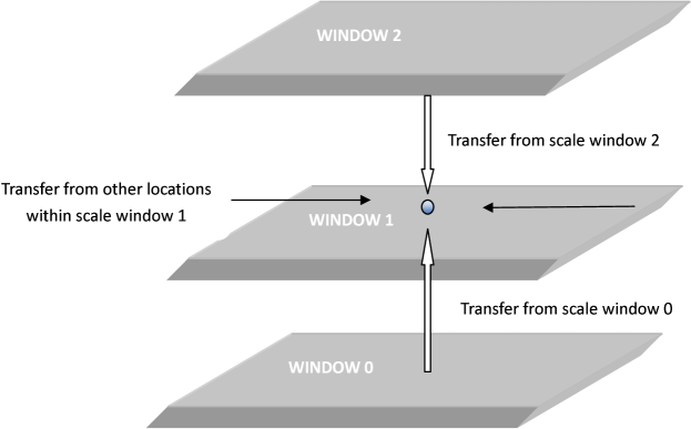
Figure 4: A schematic of the canonical energy transfer toward scale window 1.

An energy transfer process toward a certain location in a scale window involves not only the transfer from outside the window, but also those from within. This is a fundamental point where it differs from that based on the classical Fourier transform or Reynolds decomposition. Take for an example a transfer $\Gamma_{n}^{1}$ at location (step) $n$ in window $1$. As schematized in Fig. 4, it is the totality of the transfers from window 0, window 2, and those from the other different locations (the sampling space) within the same window. We need to distinguish these sub-processes in order for the window-window interactions to stand out.

As shown above, all the transfers can be written as a linear combination of terms in the form

$$\Gamma_{n}^{\varpi}={\widehat{{\cal R}}_{n}^{\sim{\varpi}}}{\widehat{\left(pq\right)}_{n}^{\sim{\varpi}}}.$$

It therefore suffices to analyze this single term. To make the presentation easier, we here just pick the particular case $\Gamma_{n}^{1}$. For a detailed treatment, see LR05, section 9. Now what we are considering is the transfer

$$\Gamma_{n}^{1} = {\widehat{{\cal R}}_{n}^{\sim{1}}}{\widehat{\left(pq\right)}_{n}^{\sim{1}}}={\widehat{{\cal R}}_{n}^{\sim{1}}}{\widehat{\left(\sum_{\omega_{1}=0}^{2}{{p}^{\sim\omega_{1}}}\sum_{\omega_{2}=0}^{2}{{q}^{\sim\omega_{2}}}\right)}_{n}^{\sim{1}}}$$

$$= {\widehat{{\cal R}}_{n}^{\sim{1}}}\left[{\widehat{\left({{p}^{\sim 0}}{{q}^{\sim 0}}\right)}_{n}^{\sim{1}}}+{\widehat{\left({{p}^{\sim 0}}{{q}^{\sim 1}}\right)}_{n}^{\sim{1}}}+{\widehat{\left({{p}^{\sim 1}}{{q}^{\sim 0}}\right)}_{n}^{\sim{1}}}\right]$$

$$+{\widehat{{\cal R}}_{n}^{\sim{1}}}\left[{\widehat{\left({{p}^{\sim 1}}{{q}^{\sim 2}}\right)}_{n}^{\sim{1}}}+{\widehat{\left({{p}^{\sim 2}}{{q}^{\sim 1}}\right)}_{n}^{\sim{1}}}+{\widehat{\left({{p}^{\sim 2}}{{q}^{\sim 2}}\right)}_{n}^{\sim{1}}}\right]$$

$$+{\widehat{{\cal R}}_{n}^{\sim{1}}}\left[{\widehat{\left({{p}^{\sim 0}}{{q}^{\sim 2}}\right)}_{n}^{\sim{1}}}+{\widehat{\left({{p}^{\sim 2}}{{q}^{\sim 0}}\right)}_{n}^{\sim{1}}}\right]$$

$$+{\widehat{{\cal R}}_{n}^{\sim{1}}}{\widehat{\left({{p}^{\sim 1}}{{q}^{\sim 1}}\right)}_{n}^{\sim{1}}}.$$

The first two terms represent the energy transfers to scale window 1 from windows 0 and 2, respectively; write them as $\Gamma_{n}^{0\to 1}$ and $\Gamma_{n}^{2\to 1}$. The two scale windows may also combine to contribute to $\Gamma_{n}^{1}$, though generally the contribution is negligible; this makes the third term, or $\Gamma_{n}^{0\oplus 2\to 1}$ for short. The last term, $\Gamma_{n}^{1\to 1}={\widehat{{\cal R}}_{n}^{\sim{1}}}{\widehat{\left({{p}^{\sim 1}}{{q}^{\sim 1}}\right)}_{n}^{\sim{1}}}$ is the transfer from window 1 itself. The major purpose of interaction analysis is, for scale window 1, to select $\Gamma_{n}^{0\to 1}$ and $\Gamma_{n}^{2\to 1}$ out of $\Gamma_{n}^{1}$.

For canonical transfers to other scale windows, the analysis results are referred to Table 6.

Table 6: Interaction analysis for $\Gamma^{0}$, $\Gamma^{1}$, and $\Gamma^{2}$.

$\Gamma^{2}$	$\Gamma^{0\to 2}$	$\Gamma^{1\to 2}$	$\Gamma^{0\oplus 1\to 2}$	$\Gamma^{2\to 2}$
$\Gamma^{1}$	$\Gamma^{0\to 1}$	$\Gamma^{2\to 1}$	$\Gamma^{0\oplus 2\to 1}$	$\Gamma^{1\to 1}$
$\Gamma^{0}$	$\Gamma^{1\to 0}$	$\Gamma^{2\to 0}$	$\Gamma^{1\oplus 2\to 0}$	$\Gamma^{0\to 0}$
Remark:	instability related	instability related	usually negligible

VII.2 Phase oscillation

The localized multiscale energetics as introduced above may reveal some spurious high-wavenumber oscillation that must be removed. This is a fundamental problem with real-valued localized transforms, which has been carefully examined by Iima in the context of shock waves and wavelet analysis. Since this is a technical issue that may prevent one from making the right interpretation, we here give it a brief introduction; details are referred to LR05.

As others, the MWT transform coefficients contain phase information, and so do the resulting multiscale energies, which are essentially the square of the coefficients. The phase information may not be obvious in the sampling space of the transform coefficients (with elements labeled by $n$) because of its discrete nature. But the disguised information may appear in the horizontal through a mechanism like Galilean transformation. (In the vertical direction it is negligible because the vertical velocity is generally very weak for geofluid flows.) To illustrate, look at (7) that defines the MWT. The characteristic frequency is $f_{c}\sim 2^{j_{2}}$ cycles over the time duration. Let the time step size be $\Delta t$, then $f_{c}\sim 1/\Delta t$. For a flow with speed $u_{0}$, the oscillation in time with $f_{c}$ will result in a oscillation in the horizontal with a wavelength $\sim u_{0}\Delta t$, i.e., a wavenumber $k_{c}\sim\frac{1}{u_{0}\Delta t}$. Let the mesh size be $\Delta x$. For a model to be numerically stable, the CFL condition requires that $\Delta t<\Delta x/u_{0}$. So the spurious oscillation has a wavenumber $k_{c}\sim O(\frac{1}{\Delta x})$.

The phase oscillation is a problem rooted in the nature of localized transforms. In our case, fortunately, it is always around the highest wavenumbers or smallest spatial scales in the spectrum, and is hence very easy to be removed using, for example, a 2D large-scale window reconstruction (like a horizontal low-pass filtering). This is in contrast to wavelet analysis: the larger the scale for a transform coefficient, the larger the scale for the spurious oscillation (see Iima ).

In real applications the spurious oscillation may not show up, just as in the MJO case which we will demonstrate in the following section. But in some unusual cases this could cause severe errors. We have shown such an example before in LR05 (see the Fig. 2 therein). The analysis is with a simulation of an observed meandering in the Iceland-Faeroe frontal region in August 1993. The mesh grid has a spacing $\Delta x=\Delta y=2.5\ {\rm km}$, and the time stepsize is 1800 s. The time series for the multiscale energetics analysis has a sampling interval of $10\Delta t$. So, by the above argument, the phase oscillation, if existing, will have a wavelength less than $10\times\Delta x=25~{}km$. Indeed, as shown in the Fig. 2a of LR05, the computed canonical transfer of APE is buried in oscillatory errors, with a wavelength of about 8 grid points or 20 km. These errors are efficiently removed through a 2D multiscale window reconstruction with a scale of 25 km; the resulting transfer is shown in their Fig.2b. (This can also be achieved efficiently using the traditional 2D low-pass filters.)

VIII Exemplification with the Madden-Julian Oscillation

The above formalism has been validated in previous publications and has seen its success in different real applications. This section is a demonstration of how it may be applied, with the Madden-Julian Oscillation (MJO) as an example. Note here it is not our intention to perform a comprehensive analysis of the MJO energetics, which will be carefully explored in a forthcoming study.

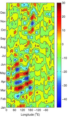
Figure 5: The 32-64 day scale window reconstruction for the 1997 OLR anomaly in the tropical area (averaged over 10^oS-10^oN). Units: $Wm^{-2}$.

MJO is a coupled convection-circulation phenomenon, manifesting itself as a localized structure of enhanced and suppressed precipitation propagating in the zonal direction at a speed of 4-8 m/s (cf. Fig. 5). It is the largest element of intraseasonal variability in the tropical atmosphere (MJO ). Though extending through the whole tropics, the anomalous rainfall occurs mainly over the Indian Ocean and Western Pacific Ocean. The oscillation has a broadband spectrum between the 30-day and 60-day periods. It is usually strong in winter and spring and weak in summer. By observation it originates over the Western Indian Ocean, becomes strengthened as it enters the Western Pacific, and dies out east of the dateline. According to Wheeler , a complete MJO cycle comprises of 8 phases, each corresponding to the position of the center of the anomalous rainfall, from Western Indian Ocean to Eastern Pacific Ocean. As an intraseasonal phenomenon, MJO bridges the large-scale and small-scale motions in the atmospheric spectrum, making an important component of the atmospheric circulation. Various studies have established its connections to tropical cyclogenesis, El Niño-Southern Oscillation, South Asia monsoon, to name a few (see MJ05 , and the references therein).

With large-scale atmospheric circulation and tropical deep convection intricately coupled, MJO provides an excellent example for the study of multiscale interaction. Analytical investigations of the interaction has been made available in the systematic work of Majda et al. (e.g., Majda04 , Majda16 ). Notice the localized and progressive pattern: It makes MJO an ideal testbed for our formalism of multiscale energetics. We are therefore using it for our purpose of demonstration.

The data we are using include those from the ECMWF Re-Analysis Interim (ERA-Interim) daily products (wind, temperature, and geopotential height), and the series of the real-time multivariate MJO (RMM) (Wheeler ). They have a spatial resolution of $2.5^{o}\times 2.5^{o}$ and span from 1988 through 2010. The vertical temperature profile, $\bar{T}=\bar{T}(p)$, which is needed in the application, is obtained by taking the time mean of $T$, followed by an averaging over all the $p$-planes.

To begin, we need to demarcate the scale windows. The problem forms a natural three-window decomposition: large-scale variabilities, MJO, and synoptic processes. We choose an MJO window of 32-64 days, since in the analysis a power of 2 for a window bound is required.

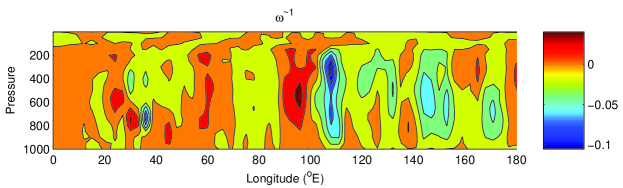
Figure 6: The equatorial $\omega=dp/dt$ on December 16, 1996, reconstructed on 32-64 day scale window. Note the up-westward tilting pattern east of the maritime continent.

We choose a strong MJO event on December 16, 1996, for our exemplification purpose. The RMM index is 2.05, corresponding to phase 5 (where the convection center is over the maritime continent). Using the above parameters, a straightforward application to the outgoing longwave radiation (OLR) in the tropical region (averaged between 10^oS and 10^oN) immediately yields an MJO window reconstruction (Fig. 5). From it the eastward propagation and its seasonal variation are clearly seen. Likewise, velocity and temperature can be reconstructed. Particularly, ${{u}^{\sim 1}}$, ${{\omega}^{\sim 1}}$, and ${{T}^{\sim 1}}$ have on the zonal cross section an up-westward tilting pattern, as identified earlier on (e.g., Moncrieff ); see Fig. 6.

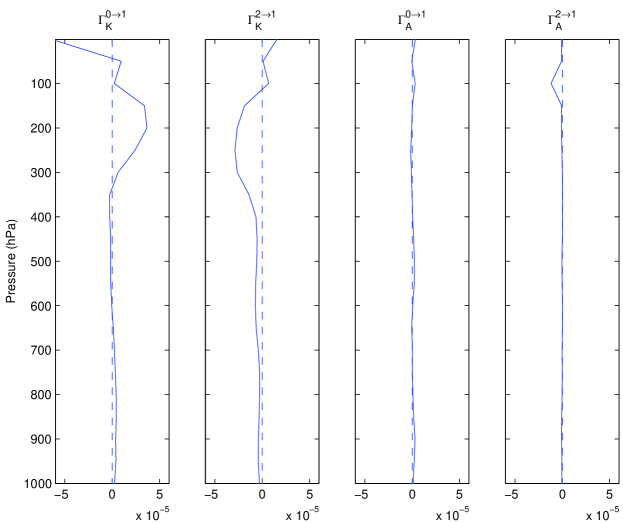
Figure 7: $\Gamma_{K}^{0\to 1}$, and $\Gamma_{K}^{2\to 1}$, $\Gamma_{A}^{0\to 1}$, and $\Gamma_{A}^{2\to 1}$ averaged between 10^oS-10^oN and 0^oE-$180^{o}$E. Units: $m^{2}/s^{3}$.

Show in Fig. 7 are the vertical distributions of the canonical transfers to the MJO window averaged over the tropical region (10^oS-10^oN) between 0^oE-180^oE. From the kinetic transfers, $\Gamma_{K}^{0\to 1}$ is on the whole positive, while $\Gamma_{K}^{2\to 1}$ is negative. That is to say, $\Gamma_{K}$ is downscale. In contrast, its potential energy counterpart tends to be more irregularly distributed, and, besides, is one order smaller. Though this is just for one particular day only, the long time mean also has the trend. This is in opposite to that for the the mid-latitude paradigm, where the canonical APE transfer is downscale while the canonical KE transfer is upscale (Saltzman70 ). From the figure the transfer center is located in the upper troposphere around 200 hPa, in agreement with the previous studies (e.g, Hsu ).

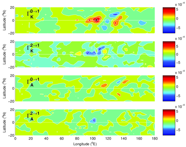
Figure 8: $\Gamma_{K}^{0\to 1}$, $\Gamma_{K}^{2\to 1}$, $\Gamma_{A}^{0\to 1}$, and $\Gamma_{A}^{2\to 1}$ at 100 hPa (units: $m^{2}/s^{3}$).

To examine the the horizontal distributions of instability centers, in Fig. 8 we draw the maps of the canonical transfers at 200 hPa. We see that they are mainly distributed between 100-140^oE, i.e., the maritime continent. This is, of course, in agreement with the phase where MJO lies at that time.

We emphasize again that it is not our intention to study the MJO dynamics here. We just pick for the demonstration purpose such an example at such an instance. It is seen that, through a straightforward application, one immediately obtains a bunch of maps of the multiscale energetics that reflect the underlying internal dynamics, and these energetics agree well with the previous studies. A detailed study of MJO the intraseasonal mode requires a statistical examination of the resulting energetics; we will see that later in Lu et al..

IX Conclusions and discussion

Multiscale energetics diagnostics are important in that they provide an approach to the fundamental problems of atmospheres and oceans like mean flow-disturbances interaction, instability and disturbance growth, etc., as identified in the National Report of Lindzen and FarrellLindzen . Their importance is also seen in the potential role that they may play in the major engineering problems such as eddy transport parameterization (e.g., Gent , Greatbatch , Visbeck , DMarshall10 ), turbulence and feedback closure (e.g., Jin ), etc. Based on the new analysis machinery namely multiscale window transform (MWT), which is capable of orthogonally decomposing a function space into a direct sum of several subspaces while retaining the local information in the resulting transform coefficients, we have given a comprehensive derivation of the multiscale energetics for the atmosphere, with respect to both the primitive equation and model quasi-geostrophic model. By taking advantage of the nice properties of the MWT, an “atomic” reconstruction of the fluxes on the multiscale windows allows for a unique separation of the inter-scale transfer from the nonlinearly intertwined energetics. The resulting transfer bears a Lie bracket form, reminiscent of the Poisson bracket in the Hamiltonian dynamics; for this reason, we call it canonical transfer. A canonical transfer sums to zero over scale windows, indicating that it is a mere redistribution of energy among the scale windows, without generating or destroying energy as a whole.

The multiscale atmospheric kinetic energy (KE) and available potential energy (APE) equations are thence derived. By classification, a multiscale energetic cycle comprises of the following processes: KE transport, APE transport, pressure work, buoyancy conversion, work done by external forcing and diabatic and frictional processes in the respective scale windows, and the interscale canonical transfers of KE and APE, which have been shown to correspond to the barotropic and baroclinic instabilitiesLR07 . Note that a buoyancy conversion takes place in an individual window only, bridging the two types of energy namely KE and APE. It does not involve the process among different scale windows, and hence basically is not related to instabilities, although traditionally it has been used to diagnose baroclinic instabilities. A brief application of the formalism is exemplified with the Madden-Julian Oscillation.

Also derived are the multiscale KE and APE equations for quasi-geostrophic flows and, for completeness, those for oceanic circulations. It should be cautioned that, since what we talk about are four-dimensional energy distribution and evolution, the term “energy” in this study is, in a strict sense, “energy density.” The abuse of terminology will not cause confusion as it is clear in the context.

It should be mentioned that the definition of APE is still an active arena of research; a recent review can be found in Tailleux . In the present formalism, APE is defined as that in Lorenz , which takes a quadratic form. However, it has been argued that it is generally not quadratic, if the 1D reference hydrostaic thermodynamic profile is achieved by adiabatic rearrangement of the existing 3D state (e.g., Holliday , Winters95 , Winters13 ). This raises an issue about how to handle an APE in non-quadratic form in the multiscale formalism. Recall that, in this study, central at the multiscale energy representation is the Parseval relation, while the relation works only for quadratic properties. For a non-quadratic APE, the problem may need to be considered from a more fundamental point of view. We will leave that to future discussions.

Notice that presented in this study is about the energetics based on a three-scale window decomposition. It is straightforward to extend the formalism to four, five, or more scale windows; the resulting energy equations are the same in form. One may equally reduce the number of windows to two.

We remark that there is a well-known apparatus in achieving a two-scale decomposition in atmospheric research, that is, the decomposition through taking transformed Eulerian mean (Andrews76 , McIntyre ; also see Plumb05 , Buhler ). Formalisms of two-scale energetics have been established with the theory (e.g., Plumb83 ). But how these formalisms may be related to that in this study is yet to be carefully examined.

In LR05, there is also a brief touch on multiscale enstrophy analysis, which makes the whole a “localized multiscale energy and vorticity analysis,” or MS-EVA for short. Since the multiscale enstrophy equation is closely related to an important concept in dynamic meteorology, namely, the Eliassen-Palm flux (Eliassen , Buhler , Vallis ), which has been extensively employed in wave-activity diagnosis and certainly deserves a detailed study for its own sake (e.g., JMarshall84 , Plumb86 , Rhines , Nakamura , Takaya ), we will defer it to another investigation in the near future.

Appendix A A glossary of notations

• ${\nabla}$: 3D gradient operator, ${\nabla}={\bf e}_{\lambda}{\frac{\partial\ }{\partial\lambda}}+{\bf e}_{\varphi}{\frac{\partial\ }{\partial\varphi}}+{\bf e}_{p}{\frac{\partial\ }{\partial p}}$

• ${\nabla_{h}}$: horizontal gradient operator (horizontal component of ${\nabla}$)

• ${\bf v}$: velocity: for atmospheres, ${\bf v}=(u,v,\omega)$, $\omega=dp/dt$; for oceans, ${\bf v}=(u,v,w)$.

• ${\bf v}_{h}=(u,v)$

• $\phi$: scaling function

• ${\widehat{\pi}^{\sim\varpi}}$: MWT of some property $\pi$ at step $n$ on window $\varpi$; dependence on $n$ is suppressed when no confusion arises

• $\pi^{\sim\varpi}$: window $\varpi$-filtered $\pi$ (multiscale window reconstruction of $\pi$ on window $\varpi$)

• $\pi_{n}^{\varpi}$: notation of some property at step $n$ on window $\varpi$; $n$ is suppressed when no confusion arises.

• $\bar{T}=\bar{T}(p)$: mean temperature profile (averaged over the $p$-plane and time)

• $T$: departure from $\bar{T}$

• $\alpha$: specific volume

• ${\Phi}$: geopotential function

• $Z$: geopotential height $(Z=\Phi/g)$

• $R$: specific gas constant (in $\rm J\cdot kg^{-1}K^{-1}$)

• $c_{p}=1.005\times 10^{3}$: specific heat capacity of air (in J/kg.K) for isobaric processes

• $c_{v}$: specific heat capacity of air for isochoric processes

• $f$: Coriolis parameter

• $\beta$: meridional gradient of $f$

• $L$: Lapse rate ($L=-\frac{\partial\bar{T}}{\partial z}$)

• $L_{d}$: Lapse rate of dry air ($L_{d}=g/c_{p}$)

• $a$: radius of Earth

• $(\lambda,\varphi,r)$: the spherical coordinates

• $p$: pressure coordinate

• $z=r-a$; $dx=a\cos\varphi d\lambda$, $dy=ad\varphi$

• $(\tilde{x},\tilde{y},\tilde{z})$: Cartesian coordinates

• ${\bf i},{\bf j},{\bf k}$: unit vectors for the cartesian coordinate system

• ${\bf e}_{\lambda},{\bf e}_{\varphi},{\bf e}_{z}$: unit vectors for spherical coordinate system

• ${\bf e}_{\lambda},{\bf e}_{\varphi},{\bf e}_{p}$: unit vectors for the isobaric spherical coordinate system

• $g$: acceleration due to gravity

• $(h_{\lambda},h_{\varphi},h_{z})$: Lamé’s coefficients

• $\bar{\rho}=\bar{\rho}(z)$: stationary density profile (ocean)

• $\rho$: density perturbation with $\bar{\rho}$ removed (ocean)

• $\rho_{0}$: chosen to be 1025 (kg/m³) here (ocean)

• $N=N(z)=\sqrt{-\frac{g}{\rho_{0}}\frac{\partial\bar{\rho}}{\partial z}}$: buoyancy frequency (ocean)

• $P$: dynamic pressure, i.e., pressure with $\bar{P}(z)=\bar{P}_{0}-\int_{0}^{z}\bar{\rho}gdz$ removed (ocean)

• $c=\frac{g}{\bar{T}(g/c_{p}-L)}$ (atmosphere); $c=\frac{g^{2}}{\rho_{0}^{2}N^{2}}$ (ocean)

• ${\bf Q}$: flux

• $\Gamma$: canonical transfer

• $A$: available potential energy

• $K$: kinetic energy

• $b$: buoyancy conversion rate

• $F_{h}$: friction/external forcing in horizontal direction

• $F_{z}$: friction/external forcing in vertical direction

• $F_{p}$: friction/external forcing in $p$ direction

• $\psi$: streamfunction

• ${\bf v}_{g}$: geostrophic velocity ($={\bf k}\times{\nabla_{h}}\psi$)

• ${F_{r}}$: rotational internal Froude number

• ${\varepsilon}$: Rossby number $(=\frac{1}{f_{0}t_{0}})$

• ${\alpha_{\ell}}=\frac{U_{0}t_{0}}{L_{0}}$

• ${\mathscr{L}}=\frac{\partial\ }{\partial t}+{\bf v}_{g}\cdot{\nabla_{h}}=\frac{\partial\ }{\partial t}+J(\psi,\ )$

Appendix B Expansion of ${\nabla}\cdot({\bf v}{\bf v})$ in spherical coordinates

To compute the canonical transfer (52), we are required to evaluate explicitly ${\nabla}\cdot({\bf v}{\bf v}_{h})$ in the spherical coordinate system ($\lambda$, $\varphi$, $r$), which are connected with the cartesian coordinates $(\tilde{x},\tilde{y},\tilde{z})$ as follows:

$$\tilde{x}=r\cos\varphi\cos\lambda,$$ (151)

$$\tilde{y}=r\cos\varphi\sin\lambda,$$ (152)

$$\tilde{z}=r\sin\varphi.$$ (153)

Here the over-tilde is employed to avoid confusing with $z$ which will be reserved for height measuring from the earth surface: $z=r-a$, with $a$ being the radius of Earth. Besides, in meteorology, $dx$ and $dy)$ are usually reserved for $a\cos\varphi d\lambda$ and $ad\varphi$, respectively. From the position vector ${\bf x}=\tilde{x}{\bf i}+\tilde{y}{\bf j}+\tilde{z}{\bf k}$ it is easy to find the Lamé’s coefficients as follows (cf. Fig. 9):

$$h_{\lambda}=\left|\frac{\partial{\bf x}}{\partial\lambda}\right|=r\cos\varphi,$$ (154)

$$h_{\varphi}=\left|\frac{\partial{\bf x}}{\partial\varphi}\right|=r,$$ (155)

$$h_{z}=\left|\frac{\partial{\bf x}}{\partial z}\right|=1.$$ (156)

With the shallow water approximation, $r\approx a={\rm const}$. So

$${\nabla}\cdot({\bf v}{\bf v})={\nabla}\cdot[{\bf v}(u{\bf e}_{\lambda}+v{\bf e}_{\varphi}+w{\bf e}_{z})]$$ (157)

$$=\frac{1}{a\cos\varphi}{\frac{\partial[u(u{\bf e}_{\lambda}+v{\bf e}_{\varphi}+w{\bf e}_{z})]}{\partial\lambda}}+\frac{1}{a\cos\varphi}{\frac{\partial[v(u{\bf e}_{\lambda}+v{\bf e}_{\varphi}+w{\bf e}_{z})\cos\varphi]}{\partial\varphi}}$$ (158)

$$\quad+\frac{\partial[w(u{\bf e}_{\lambda}+v{\bf e}_{\varphi}+w{\bf e}_{z})]}{\partial z}.$$ (159)

And, particularly,

$${\nabla}\cdot({\bf v}{\bf v}_{h})={\nabla}\cdot[{\bf v}(u{\bf e}_{\lambda}+v{\bf e}_{\varphi})]$$ (160)

$$=\frac{1}{a\cos\varphi}{\frac{\partial[u(u{\bf e}_{\lambda}+v{\bf e}_{\varphi})]}{\partial\lambda}}+\frac{1}{a\cos\varphi}{\frac{\partial[v(u{\bf e}_{\lambda}+v{\bf e}_{\varphi})\cos\varphi]}{\partial\varphi}}$$ (161)

$$\quad+\frac{\partial[w(u{\bf e}_{\lambda}+v{\bf e}_{\varphi})]}{\partial z}.$$ (162)

We need to evaluate ${\frac{\partial{\bf e}_{\lambda}}{\partial\lambda}}$, ${\frac{\partial{\bf e}_{\lambda}}{\partial\varphi}}$, etc.

There are several ways to achieve the evaluation. One may do it by directly taking the limit ${\frac{\partial{\bf e}_{\lambda}}{\partial\lambda}}=\lim_{\Delta\lambda\to 0}\frac{\Delta{\bf e}_{\lambda}}{\Delta\lambda}.$ Another way is to first connect $({\bf e}_{\lambda},{\bf e}_{\varphi},{\bf e}_{z})$ with $({\bf i},{\bf j},{\bf k})$, then take the derivatives. Besides, one may take advantage of the properties such as:

$${\bf e}_{\lambda}\cdot{\bf e}_{\varphi}=1\Longrightarrow\partial{\bf e}_{\lambda}\cdot{\bf e}_{\lambda}=0\Longrightarrow\partial{\bf e}_{\lambda}\perp{\bf e}_{\lambda}.$$

From Fig. 9, it is easy to find that

$${\bf e}_{\lambda}=-\sin\lambda{\bf i}+\cos\lambda{\bf j},$$ (163)

$${\bf e}_{\varphi}=-\sin\varphi\cos\lambda{\bf i}-\sin\varphi\sin\lambda{\bf j}+\cos\varphi{\bf k},$$ (164)

$${\bf e}_{z}=\cos\varphi\cos\lambda{\bf i}+\cos\varphi\sin\lambda{\bf j}+\sin\varphi{\bf k}.$$ (165)

Inverting,

$${\bf i}=-\cos\lambda\sin\varphi{\bf e}_{\varphi}+\cos\lambda\cos\varphi{\bf e}_{z}-\sin\lambda{\bf e}_{\lambda},$$ (166)

$${\bf j}=-\sin\lambda\sin\varphi{\bf e}_{\varphi}+\sin\lambda\cos\varphi{\bf e}_{z}+\cos\lambda{\bf e}_{\lambda},$$ (167)

$${\bf k}=\cos\varphi{\bf e}_{\varphi}+\sin\varphi{\bf e}_{z}.$$ (168)

So

$${\frac{\partial{\bf e}_{\lambda}}{\partial\lambda}}=-\cos\lambda{\bf i}-\sin\lambda{\bf j}=\sin\varphi{\bf e}_{\varphi}-\cos\varphi{\bf e}_{z},$$ (169)

$${\frac{\partial{\bf e}_{\lambda}}{\partial\varphi}}=0,$$ (170)

$$\frac{\partial{\bf e}_{\lambda}}{\partial z}=0,$$ (171)

$${\frac{\partial{\bf e}_{\varphi}}{\partial\lambda}}=\sin\varphi\sin\lambda{\bf i}-\sin\varphi\cos\lambda{\bf j}=-\sin\varphi{\bf e}_{\lambda},$$ (172)

$${\frac{\partial{\bf e}_{\varphi}}{\partial\varphi}}=-\cos\varphi\cos\lambda{\bf i}-\cos\varphi\sin\lambda{\bf j}-\sin\varphi{\bf k}=-{\bf e}_{z},$$ (173)

$$\frac{\partial{\bf e}_{\varphi}}{\partial z}=0,$$ (174)

$${\frac{\partial{\bf e}_{z}}{\partial\lambda}}=-\cos\varphi\sin\lambda{\bf i}+\cos\varphi\cos\lambda{\bf j}=\cos\varphi{\bf e}_{\lambda},$$ (175)

$${\frac{\partial{\bf e}_{z}}{\partial\varphi}}=-\sin\varphi\cos\lambda{\bf i}-\sin\varphi\sin\lambda{\bf j}+\cos\varphi{\bf k}={\bf e}_{\varphi},$$ (176)

$$\frac{\partial{\bf e}_{z}}{\partial z}=0.$$ (177)

Also one may obtain:

$$\frac{d{\bf e}_{\lambda}}{dt}=\frac{u}{a\cos\varphi}({\bf e}_{\varphi}\sin\varphi-{\bf e}_{z}\cos\varphi),$$ (178)

$$\frac{d{\bf e}_{\varphi}}{dt}=\frac{u\tan\varphi}{a}{\bf e}_{\lambda}-\frac{v}{a}{\bf e}_{z},$$ (179)

$$\frac{d{\bf e}_{z}}{dt}=\frac{u}{a}{\bf e}_{\lambda}+\frac{v}{a}{\bf e}_{z}.$$ (180)

With the above results, (159) now can be expanded as

$${\nabla}\cdot({\bf v}{\bf v}) = \frac{1}{a\cos\varphi}\left[{\frac{\partial u^{2}}{\partial\lambda}}{\bf e}_{\lambda}+{\frac{\partial uv}{\partial\lambda}}{\bf e}_{\varphi}+{\frac{\partial uw}{\partial\lambda}}{\bf e}_{z}+u^{2}{\frac{\partial{\bf e}_{\lambda}}{\partial\lambda}}+uv{\frac{\partial{\bf e}_{\varphi}}{\partial\lambda}}+uw{\frac{\partial{\bf e}_{z}}{\partial\lambda}}\right]$$ (181)

$$+ \frac{1}{a\cos\varphi}\left[{\frac{\partial(vu\cos\varphi)}{\partial\varphi}}{\bf e}_{\lambda}+{\frac{\partial(v^{2}\cos\varphi)}{\partial\varphi}}{\bf e}_{\varphi}+{\frac{\partial(vw\cos\varphi)}{\partial\varphi}}{\bf e}_{z}\right.$$ (182)

$$\qquad+\left.vu\cos\varphi{\frac{\partial{\bf e}_{\lambda}}{\partial\varphi}}+v^{2}\cos\varphi{\frac{\partial{\bf e}_{\varphi}}{\partial\varphi}}+vw\cos\varphi{\frac{\partial{\bf e}_{z}}{\partial\varphi}}\right]$$ (183)

$$+ \left[\frac{\partial wu}{\partial z}{\bf e}_{\lambda}+\frac{\partial wv}{\partial z}{\bf e}_{\varphi}+\frac{\partial w^{2}}{\partial z}{\bf e}_{z}+wu\frac{\partial{\bf e}_{\lambda}}{\partial z}+wv\frac{\partial{\bf e}_{\varphi}}{\partial z}+w^{2}\frac{\partial{\bf e}_{z}}{\partial z}\right]$$ (184)

Or,

$${\nabla}\cdot({\bf v}{\bf v})=\left\{\frac{1}{a\cos\varphi}\left[{\frac{\partial u^{2}}{\partial\lambda}}-uv\sin\varphi+uw\cos\varphi+{\frac{\partial(vu\cos\varphi)}{\partial\varphi}}\right]+\frac{\partial wu}{\partial z}\right\}{\bf e}_{\lambda}$$ (185)

$$\quad+\left\{\frac{1}{a\cos\varphi}\left[{\frac{\partial uv}{\partial\lambda}}+u^{2}\sin\varphi+{\frac{\partial(v^{2}\cos\varphi)}{\partial\varphi}}+vw\cos\varphi\right]+\frac{\partial wv}{\partial z}\right\}{\bf e}_{\varphi}$$ (186)

$$\quad+\left\{\frac{1}{a\cos\varphi}\left[{\frac{\partial uw}{\partial\lambda}}-u^{2}\cos\varphi+{\frac{\partial(vw\cos\varphi)}{\partial\varphi}}-v^{2}\cos\varphi\right]+\frac{\partial w^{2}}{\partial z}\right\}{\bf e}_{z}.$$ (187)

One may check that, with the aid of the incompressibility assumption

$$\frac{1}{a\cos\varphi}{\frac{\partial u}{\partial\lambda}}+\frac{1}{a\cos\varphi}{\frac{\partial v\cos\varphi}{\partial\varphi}}+\frac{\partial w}{\partial z}=0,$$

the above equation is equivalent to

$$\left(\frac{u}{a\cos\varphi}{\frac{\partial u}{\partial\lambda}}+\frac{v}{a}{\frac{\partial u}{\partial\varphi}}+w\frac{\partial u}{\partial z}-\frac{uv}{a}\tan\varphi+\frac{uw}{a}\right){\bf e}_{\lambda}$$

$$+\left(\frac{u}{a\cos\varphi}{\frac{\partial v}{\partial\lambda}}+\frac{u^{2}}{a}\tan\varphi+\frac{v}{a}{\frac{\partial v}{\partial\varphi}}+\frac{vw}{a}+w\frac{\partial v}{\partial z}\right){\bf e}_{\varphi}$$

$$+\left(\frac{u}{a\cos\varphi}{\frac{\partial w}{\partial\lambda}}+\frac{v}{a}{\frac{\partial w}{\partial\varphi}}+w\frac{\partial w}{\partial z}-\frac{u^{2}+v^{2}}{a}\right){\bf e}_{z},$$

which is precisely the advection part in the non-approximated momentum equations in spherical coordinates. Eq. (187) is thence verified.

As a particular case,

$${\nabla}\cdot({\bf v}{\bf v}_{h}) = \frac{1}{a\cos\varphi}\left[{\frac{\partial u^{2}}{\partial\lambda}}{\bf e}_{\lambda}+{\frac{\partial uv}{\partial\lambda}}{\bf e}_{\varphi}+u^{2}{\frac{\partial{\bf e}_{\lambda}}{\partial\lambda}}+uv{\frac{\partial{\bf e}_{\varphi}}{\partial\lambda}}\right]$$ (188)

$$+ \frac{1}{a\cos\varphi}\left[{\frac{\partial(vu\cos\varphi)}{\partial\varphi}}{\bf e}_{\lambda}+{\frac{\partial(v^{2}\cos\varphi)}{\partial\varphi}}{\bf e}_{\varphi}\right.$$ (189)

$$\qquad+\left.vu\cos\varphi{\frac{\partial{\bf e}_{\lambda}}{\partial\varphi}}+v^{2}\cos\varphi{\frac{\partial{\bf e}_{\varphi}}{\partial\varphi}}\right]$$ (190)

$$+ \left[\frac{\partial wu}{\partial z}{\bf e}_{\lambda}+\frac{\partial wv}{\partial z}{\bf e}_{\varphi}+wu\frac{\partial{\bf e}_{\lambda}}{\partial z}+wv\frac{\partial{\bf e}_{\varphi}}{\partial z}\right]$$ (191)

Or,

$${\nabla}\cdot({\bf v}{\bf v}_{h})=\left\{\frac{1}{a\cos\varphi}\left[{\frac{\partial u^{2}}{\partial\lambda}}-uv\sin\varphi+{\frac{\partial(vu\cos\varphi)}{\partial\varphi}}\right]+\frac{\partial wu}{\partial z}\right\}{\bf e}_{\lambda}$$ (192)

$$\quad+\left\{\frac{1}{a\cos\varphi}\left[{\frac{\partial uv}{\partial\lambda}}+u^{2}\sin\varphi+{\frac{\partial(v^{2}\cos\varphi)}{\partial\varphi}}\right]+\frac{\partial wv}{\partial z}\right\}{\bf e}_{\varphi}$$ (193)

$$\quad+\left\{\frac{1}{a\cos\varphi}\left[-u^{2}\cos\varphi-v^{2}\cos\varphi\right]\right\}{\bf e}_{z}.$$ (194)

Correspondingly with the incompressibility assumption this is,

$$\left(\frac{u}{a\cos\varphi}{\frac{\partial u}{\partial\lambda}}+\frac{v}{a}{\frac{\partial u}{\partial\varphi}}+w\frac{\partial u}{\partial z}-\frac{uv}{a}\tan\varphi\right){\bf e}_{\lambda}$$

$$+\left(\frac{u}{a\cos\varphi}{\frac{\partial v}{\partial\lambda}}+\frac{u^{2}}{a}\tan\varphi+\frac{v}{a}{\frac{\partial v}{\partial\varphi}}+w\frac{\partial v}{\partial z}\right){\bf e}_{\varphi}$$

$$+\left(-\frac{u^{2}+v^{2}}{a}\right){\bf e}_{z}.$$

Appendix C Some quasi-geostrophic results used in the text

Using the scaling in section VI, it is easy to have the scaled inviscid governing equations (103)-(106) as follows (now all the variables in this appendix are understood as nondimensional):

$${\varepsilon}\frac{\partial{\bf v}_{h}}{\partial t}+{\varepsilon}{\alpha_{\ell}}\left({\bf v}_{h}\cdot{\nabla_{h}}{\bf v}_{h}+w\frac{\partial{\bf v}_{h}}{\partial z}\right)+f{\bf k}\times{\bf v}_{h}=-{\nabla_{h}}P$$ (195)

$$\rho=-\frac{\partial P}{\partial z}$$ (196)

$${\nabla_{h}}\cdot{\bf v}_{h}+\frac{\partial w}{\partial z}=0$$ (197)

$${F_{r}}^{2}{\varepsilon}\frac{\partial\rho}{\partial t}+{F_{r}}^{2}{\varepsilon}{\alpha_{\ell}}\left({\bf v}_{h}\cdot{\nabla_{h}}\rho+w\frac{\partial\rho}{\partial z}\right)=N^{2}w$$ (198)

where $f=1+{\varepsilon}\beta y$.

Expanding $P$, $w$, ${\bf v}_{h}$, and $\rho$ in the power of ${\varepsilon}$, as that in (132)-(135), it is easy to show that

$$[{\bf v}_{h}]_{0}={\bf k}\times{\nabla}[P]_{0},$$ (199)

$$[w]_{0}=0.$$ (200)

$$[\rho]_{0}=-\frac{\partial[P]_{0}}{\partial z}$$ (201)

and

$$[w]_{1}=-\frac{{F_{r}}^{2}}{N^{2}}{\mathscr{L}}\left(\frac{\partial[P]_{0}}{\partial z}\right),$$ (202)

$$[{\bf v}_{h}]_{1}={\bf k}\times{\mathscr{L}}([{\bf v}_{h}]_{0})-\beta y[{\bf v}_{h}]_{0}+{\bf k}\times{\nabla_{h}}[P]_{1},$$ (203)

where $\mathscr{L}$ is the substantial differential operator along the geostrophic flow $[{\bf v}_{h}]_{0}$: $\mathscr{L}=\frac{\partial\ }{\partial t}+[{\bf v}_{h}]_{0}\cdot{\nabla_{h}}$. Eqs. (199) - (203) are to be used in the text in section VI.

As conventional, let $[P]_{0}\equiv\psi$. Following the derivations in standard textbooks (e.g., McWilliams_book ), we have

$$\frac{\partial\ }{\partial t}\left[{\nabla_{h}}^{2}\psi+\frac{\partial\ }{\partial z}\left(\frac{{F_{r}}^{2}}{N^{2}}\frac{\partial\psi}{\partial z}\right)\right]+{\alpha_{\ell}}J\left(\psi,\ \left[{\nabla_{h}}^{2}\psi+\frac{\partial\ }{\partial z}\left(\frac{{F_{r}}^{2}}{N^{2}}\frac{\partial\psi}{\partial z}\right)\right]\right)+\beta\frac{\partial\psi}{\partial x}=0,$$ (204)

where $J$ is the Jacobian operator. This is the very quasi-geostrophic equation for which we derive the multiscale energetics.

Figure 9: Spherical coordinate frame.

References

- (1) Andrews, D.G., and M.E. McIntyre, 1976: Planetary waves in horizontal and vertical shear: The generalized Eliassen-Palm relation and the mean zonal acceleration. J. Atmos. Sci., 33, 2031-2048.
- (2) Berloff, P.S., 2005: On dynamically consistent eddy fluxes. Dyn. Atmos. Oceans, 38, 123-146.
- (3) Boyd, J., 1976: The noninteraction of waves with the zonally-averaged flow on a spherical Earth and the interrelationships of eddy fluxes of energy, heat and momentum. J. Atmos. Sci. 33, 2285-2291.
- (4) Bühler, O., 2009: Waves and Mean Flows. Cambridge University Press.
- (5) Cai, M., and M. Mak, 1990: On the basic dynamics of regional cyclogenesis. J. atmos. Sci., 47 (12), 1417-1442.
- (6) Cai, M., S. Yang, H.M. Van Den Dool, and V.E. Kousky, 2007: Dynamical implications of the orientation of atmospheric eddies: a local energetics perspective. Tellus, 59A, 127-140.
- (7) Chapman, C.C., A.M. Hogg, A.E. Kiss, and S.R. Rintoul, 2015: The dynamics of southern ocean storm tracks. J. Phys. Oceanogr., 45, 884-903.
- (8) Charney, J.G., and P.G. Drazin, 1961: Propagation of planetary-scale disturbances from the lower into the upper atmosphere. J. Geophys. Res., 66(1), 83-109.
- (9) Chen, R., G.R. Flier, and C. Wunsch, 2014: A description of local and nonlocal eddy-mean flow interaction in a globally eddy-permitting state estimate. J. Phys. Oceanogr., 44, 2336-2352.
- (10) Chorin, A.J., 1994: Vorticity and Turbulence. Springer-Verlag, New York. 173pp.
- (11) Cronin, M., and R. Watts, 1996: Eddy-mean flow interaction in the Gulf Stream at 68W. Part I: Eddy energetics. J. Phys. Oceanogr., 26, 2107-2131.
- (12) Dewar, W.K., and J.M. Bane, 1989: Gulf Stream dynamics. Part II. Eddy energetics at 73 W. J. Phys. Oceanogr., 19, 1574-1587.
- (13) Dickinson, Robert E., 1969: Theory of planetary wave-zonal flow interaction. J. atmos. Sci., 26, 73-81.
- (14) Eliassen, Arnt, and Enok Palm, 1961: On the transfer of energy in stationary mountain waves. Geofys. Publikasjoner, 22, 1-23.
- (15) Farge, M., 1992: Wavelet transforms and their applications to turbulence. Annu. Rev. Fluid Mech., 24, 395-457.
- (16) Fels, S.B., and R.S. Lindzen, 1974: The interaction of thermally excited gravity waves with mean flows. Geophys. Fluid Dyn., 6, 149-191.
- (17) Fournier, A., 2001: Atmospheric energetics in the wavelet domain. Part I: Governing equations and interpretation for idealized flows. J. Atmos. Sci., 59, 1182-1197.
- (18) Gent, P.R., and J.C. McWilliams, 1990: Isopycnal mixing in ocean circulation models. J. Phys. Oceanogr., 20, 150-160.
- (19) Greatbatch, R.J., 1998: Exploring the relationship between eddy-induced transport velocity, vertical momentum transfer, and the isopycnal flux of potential vorticity. J. Phys. Oceanogr., 28, 422-432.
- (20) Haidvogel, D., J.C. McWilliams, and P. Gent, 1992: Boundary current separation in a quasi-geostrophic, eddy-resolving ocean circulation model. J. Phys. Oceanogr., 22, 882-902.
- (21) Harrison, D.E., and A.R. Robinson, 1978: Energy analysis of open regions of turbulent flows-mean eddy energetics of a numerical ocean circulation experiment. Dyn. Atmos. Oceans, 2, 185-211.
- (22) Haynes, Peter H., 1988: Forced, dissipative generalizations of finite-amplitude wave-activity conservation relations for zonal and nonzonal basic flows. J. Atmos. Sci., 45, 2352-2362.
- (23) Holland, W.R., 1978: The role of mesoscale eddies in the general circulation of the ocean–Numerical experiments using a wind-driven quasi-geostrophic model. J. Phys. Oceanogr., 8, 363-392.
- (24) Holliday, D., and M.E. McIntyre, 1981: On potential energy density in an imcompressible, stratified fluid. J. Fluid Mech., 107, 221-225.
- (25) Holopainen, E.O., 1978: A diagnostic study on the kinetic energy balance of the long-term mean flow and the associated transient fluctuations in the atmosphere. Geophysica, 15, 125-145.
- (26) Hoskins, Brian J., I.N. James, and G.H. White, 1983: The shape, propagation and mean-flow interaction of large-scale weather systems. J. Atmos. Sci., 40, 1595-1612.
- (27) Hsu, P.-C., T. Li, and C.-H. Tsou, 2011: Interactions between boreal summer intraseasonal oscillations and synoptic-scale disturbances over the Western North Pacific. Part I: Energetics diagnosis. J. Clim. 24, 927-941.
- (28) Huang, N.E., Z. Shen, and S.R. Long, 1999: A new view of nonlinear water waves: The Hilbert spectrum. Annu. Rev. Fluid Mech., 31, 417-457.
- (29) Iima, M., and S. Toh, 1995: Wavelet analysis of the energy transfer caused by convective terms: Application to the Burgers shock. Phys. Rev. E 52(6), 6189-6201.
- (30) Ingersoll, A.P., 2005: Boussinesq and anelastic approximations revisited: potential energy release during thermobaric instability. J. Phys. Oceanogr., 35 1359-1369.
- (31) Jin, F.-F., 2010: Eddy-induced instability for low-frequency variability. J. Atmos. Sci., 67, 1947-1964.
- (32) Kao, S.-K., 1968: Governing equations and spectra for atmospheric motion and transports in frequency, wave-number space. J. Atmos. Sci., 25, 32-38.
- (33) Li, Chongyin, Zhenxia Long, 2001: Intraseasonal oscillation anomalies in the tropical atmosphere and the 1997 El Nino occurrence. Chinese J. Atmos. Sci., 25, 337-345.
- (34) Liang, X.S., and M. Wang, 2004: A study of turbulent wakes using a novel localized stability analysis. Proc. Center for Turbulence Research Summer Program 2004, Stanford, CA, Stanford-NASA Ames Research Center, 211-222.
- (35) Liang, X.S., and A. R. Robinson, 2005: Localized multiscale energy and vorticity analysis. I. Fundamentals. Dyn. Atmos. Oceans, 38, 195-230.
- (36) Liang, X.S., and D.G.M. Anderson, 2007: Multiscale window transform. SIAM J. Multiscale Model. Simul., 6(2), 437-467.
- (37) Liang, X.S., and A.R. Robinson, 2007: Localized multiscale energy and vorticity analysis. II. Finite-amplitude instability theory and validation. Dyn. Atmos. Oceans, 44, 51-76.
- (38) Liang, X.S., and A.R. Robinson, 2009: Multiscale processes and nonlinear dynamics of the circulation and upwelling events off Monterey Bay. J. Phys. Oceanogr., 39, 290-313.
- (39) Lindzen, R.S., and B. Farrell, 1987: Atmospheric dynamics: US National report to International Union of Geodesy and Geophysics 1983-1986. Rev. Geophys., 25, 323-328.
- (40) Lorenz, Edward N., 1955: Available potential energy and the maintenance of the general circulation. Tellus VII, 2, 157-167.
- (41) Luo, Dehai, J. Cha, L. Zhong, A. Dai, 2014: A nonlinear multiscale interaction model for atmospheric blocking: The eddy-blocking matching mechanism. Quart. J. Royal Meteorol. Soc., 140, 1785-1808.
- (42) Madden, R.A., P.R. Julian, 1971: Detection of a 40-50 day oscillation in the zonal wind in the tropical Pacific. J. Atmos. Sci., 28, 702-708.
- (43) Madden, R.A., P.R. Julian, 2005: Historical Perspective. In: Intraseasonal variability in the atmosphere-ocean climate system. K.M. Lau and D.E. Waliser, eds., Praxis, 1-18.
- (44) Majda, A.J., and J.A. Biello, 2004: A multiscale model for tropical intraseasonal oscillations. Proc. Natl. Acad. Sci. USA, 101, 4736-4741.
- (45) Majda, A.J., and Q. Yang, 2016: A multiscale model for the intraseasonal impact of the diurnal cycle over the maritime continent on the Madden-Julian Oscillation. J. Atmos. Sci., 73, 579-604.
- (46) Marshal, J.C., 1984: Eddy-mean-flow interaction in a barotropic ocean model. Quart. J. R. Met. Soc., 110, 573-590.
- (47) Marshall, D.P., and A.J. Adcroft, 2010: Parameterization of ocean eddies: Potential vorticity mixing, energetics and Arnold’s first stability theorem. Ocean Modelling, 32, 188-204.
- (48) Matsuno, T., 1971: A dynamical model of the stratospheric sudden warming. J. Atmos. Sci., 28, 1479-1494.
- (49) McIntyre, M.E., 1980: An introduction to the generalized Lagrangian-mean description of wave, mean-flow interaction. Pageoph., 118, Birkauser Verlag, Basel. 152-176.
- (50) McWilliams, J.C., and J.M. Restrepo, 1999: The wave-driven ocean circulation. J. Phys. Oceanogr., 29, 2523-2540.
- (51) McWilliams, James C., 2006: Fundamentals of Geophysical Fluid Dynamics. Cambridge University Press, Cambridge, UK. 249pp.
- (52) Moncrieff, M.W., 2004: Analytic representation of the large-scale organization of tropical convection. J. Atmos. Sci., 61, 1521-1538.
- (53) Murakami, Shigenori, 2011: Atmospheric local energetics and energy interactions between mean and eddy fields. Part I: Theory. J. Atmos. Sci., 68, 760-768.
- (54) Nakamura, N., and A. Solomon, 2010: Finite-amplitude wave activity and mean flow adjustments in the atmospheric general circulation. Part I. Quasi-geostrophic theory and analysis. J. Atmos. Sci., 67, 3967-3983.
- (55) Pedlosky, J., 1987: Geophysical Fluid Dynamics. Springer-Verlag, New York, 710 pp.
- (56) Pinardi, N., and A.R. Robinson, 1986: Quasigeostrophic energetics of open ocean regions. Dyn. Atmos. Oceans 10, 185-219.
- (57) Plumb, R. Alan, 1983: A new look at the energy cycle. J. Atmos. Sci. 40, 1669-1688.
- (58) Plumb, R.A., 1986: Three-dimensional propagation of transient quasi-geostrophic eddies and its relationship with the eddy forcing of the time-mean flow. J. Atmos. Sci., 43, 1657-1678.
- (59) Plumb, R.A., and R. Ferrari, 2005: Transformed Eulerian-mean theory. Part I: Nonquasigeostrophic theory for eddies on a zonal-mean flow. J. Phys. Oceanogr., 35, 165-174.
- (60) Pope, S.B., 2004: Turbulent Flows. Cambridge University Press, Cambridge, UK. 771 pp.
- (61) Rhines, Peter B., and W.R. Holland, 1979: A theoretical discussion of eddy-driven mean flows. Dyn. Atmos. Oceans, 3: 289-325.
- (62) Salby, Murry L., 1996: Fundamentals of Atmospheric Physics. Academic Press, San Diego, CA.
- (63) Saltzman, Barry, 1957: Equations governing the energetics of the larger scales and atmospheric turbulence in the domain of wave number. J. Meteorol., 14, 513-523.
- (64) Saltzman, B., 1970: Large-scale atmospheric energetics in the wave-number domain. Rev. Geophys. Space Phys., 8, 289-302.
- (65) Sheng, J., and Y. Hayashi, 1990: Estimation of atmospheric energetics in the frequency domain during the FGGE year. J. Atmos. Sci., 47, 1255-1268.
- (66) Strang, G., and T. Nguyen, 1997: Wavelets and Filter Banks. Wellesley-Cambridge Press, Wellesley, MA, 520pp.
- (67) Su, Z., A.P. Ingersoll, A.L. Steward, A.F. Thompson, 2016: Ocean convective available potential energy. Part II: Energetics of thermobaric convection and thermobaric cabbeling. J. Phys. Oceanogr., 46, 1097-1115.
- (68) Tailleux, Rémi, 2013: Available potential energy and energy in stratified fluids. Annu. Rev. Fluid Mech., 45, 35-58.
- (69) Takaya, K., and H. Nakamura, 2001: A formulation of a phase-independent wave-activity flux for stationary and migratory quasigeostrophic eddies on a zonally varying basic flow. J. Atmos. Sci., 58, 608-627.
- (70) Trenberth, Kevin E., 1986: An assessment of the impact of transient eddies on the zonal flow during a blocking episode using localized Eliassen-Palm flux diagnostics. J. Atmos. Sci. 43, 2070-2087.
- (71) Vallis, G.K., 2006: Atmospheric and Oceanic Fluid Dynamics. Cambridge University Press, Cambridge, UK, 745pp.
- (72) Visbeck, M., J. Marshall, T. Haine, and M. Spall, 1997: Specification of eddy transfer coefficients in coarse-resolution ocean circulation models. J. Phys. Oceanogr., 27, 381-402.
- (73) Waterman, S., S.R. Jayne, 2011: Eddy-mean flow interactions in the along-stream development of a western boundary current jet: an idealized model study. J. Phys. Oceanogr., 41, 682-707.
- (74) Wheeler, M.C., and H.H. Hendon, 2004: An all-season real-time multivariate MJO index: Development of an index for monitoring and prediction. Mon. Wea. Rev. 132(8), 1917-1932.
- (75) Winters, K., P. Lombard, J. Riley, and E. D’Asaro, 1995: Available potential energy and mixing in density-stratified fluids. J. Fluid Mech., 289, 115-128.
- (76) Winters, K., and Barkan, 2013: Available potential energy density for Boussinesq fluid flow. J. Fluid Mech., 714, 476-488.