Re-iterated multiscale model reduction using the GMsFEM

Abstract

Numerical homogenization and multiscale finite element methods construct effective properties on a coarse grid by solving local problems and extracting the average effective properties from these local solutions. In some cases, the solutions of local problems can be expensive to compute due to scale disparity. In this setting, one can basically apply a homogenization or multiscale method re-iteratively to solve for the local problems. This process is known as re-iterated homogenization and has many variations in the numerical context. Though the process seems to be a straightforward extension of two-level process, it requires some careful implementation and the concept development for problems without scale separation and high contrast. In this paper, we consider the Generalized Multiscale Finite Element Method (GMsFEM) and apply it iteratively to construct its multiscale basis functions. The main idea of the GMsFEM is to construct snapshot functions and then extract multiscale basis functions (called offline space) using local spectral decompositions in the snapshot spaces. The extension of this construction to several levels uses snapshots and offline spaces interchangebly to achieve this goal. At each coarse-grid scale, we assume that the offline space is a good approximation of the solution and use all possible offline functions or randomization as boundary conditions and solve the local problems in the offline space at the previous (finer) level, to construct snapshot space. We present an adaptivity strategy and show numerical results for flows in heterogeneous media and in perforated domains.

1 Introduction

Many problems with multiple scales can have a large scale disparity. For example, porous media problems can have spatial variations from the pore-scale sizes to the field scales. Solving these problems requires coarsening approaches. Some successful coarsening methods include homogenization [3, 2, 37], numerical homogenization and generalization [49, 17, 28, 23, 27, 30, 38], and multiscale methods [28, 18, 1, 45, 36, 23, 24, 22, 29, 8, 26, 25, 33, 43, 13, 7, 34, 11]. The objective of these approaches is to solve the problem on a prescribed computational grid, which we will call the coarse grid. The coarse grid can typically be much larger than the fine grid, which resolves the underlying processes. These coarse-grid techniques require local computations to extract effective properties. In numerical homogenization methods, this involves solving cell problems. In multiscale methods, this involves solving multiscale basis functions, where multiscale basis functions play a role of effective properties [8]. In problems with very large disparate scales, the solution of local problem can be expensive and require coarsening.

There have been several approaches to approximate the local solutions, when there is very large scale disparity. The commonly used technique, which motivates our studies, is re-iterated homogenization, which goes back to [3], see also [16, 39]. Other methods include hierarchical basis functions [35, 46], hierarchical model reduction [50, 28, 31], multilevel approaches for multiscale basis functions [40, 42, 41], hierarchical upscaling [6, 32, 44], multilevel approximations [4, 5, 47, 48, 21], and approximate basis computations [19]. In these approaches, multiscale basis functions or local solutions are approximated in a re-iterated fashion by constructing multiple level approximations for the basis functions. The accuracy of local solutions may or may not have a large effect on the accuracy of the coarse-grid solutions due to subgrid errors dependent on how accurate localized approaches. These approximate local techniques can demonstrate an efficiency and speed-up in practical computations in many situations. However, these multiscale approaches construct a limited number of basis functions in each coarse block and mainly focus on designing an approximation step for calculating pre-defined local problems. Our objective is to extend a systematic approach proposed in [20, 8] in a re-iterated fashion and show that one can provide a systematic way of eliminating the degrees of freedom using snapshots and local spectral problems.

To describe the main idea of the proposed method, we briefly mention the underlying concept of the GMsFEM. The main idea of the GMsFEM is to introduce snapshots on a coarse grid and identify dominant modes in the snapshot space. The snapshot space represents a set of functions that can be used to accurately calculate the local solution space. The snapshots typically consist of local solutions with all possible boundary conditions or with randomized boundary conditions, which represent point sources distributed on the boundaries. The snapshot vectors are similar to the snapshots used in global model reduction [8]; however, they are constructed without solving expensive global problems and similar to cell problems in homogenization. The snapshot vectors are computed either by using all boundary conditions or by using random boundary conditions [8]. To avoid effects due to oscillations of random boundary conditions and improve the accuracy, we use oversampling techniques and compute snapshots in domains slightly larger than the target coarse block. The local spectral decomposition is performed in the snapshot space by identifying local spectral decomposition based on the analysis. The analysis consists of decomposing the error into local regions and bounding these error components. Furthermore, adaptivity is used to identify the regions that require more basis functions.

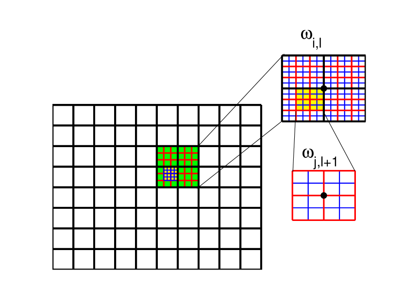
Figure 2: Mesh

Extending this approach to several disparate scale setups requires repeating the above process. Assume that we have a hierarchy of coarse meshes $H_{1}>H_{2}>...>H_{N}=h$, where our objective is to compute multiscale basis functions on the coarse grid $H_{1}$ (see Figure 2 for illustration). Here, for simplicity, $H_{l}$ denotes the mesh size, also referred to as a mesh configuration. The main contribution in extending two-level approaches to the multi-level is to identify snapshots at each level. We depict an illustration of the main concepts in Figure 1. In this regard, we define snapshots as the spaces spanned by the offline spaces (constructed via local spectral decomposition) at the previous step. More precisely, at the finest coarse-grid level, we first identify local solutions with randomized boundary conditions. The span of these local solutions defines the snapshot space, $V_{\text{snap}}^{N-1}$. Furthermore, we identify the local spectral problems and identify multiscale basis functions. We call the space spanned by multiscale basis functions the offline space and denote the $V_{\text{off}}^{N-1}$. These functions are assumed to represent the solution at the $H_{N-1}$ grid. The snapshots at the $H_{N-2}$ grid can be defined as functions, which span all functions in the offline space, $V_{\text{off}}^{N-1}$. However, one solves local problems in $V_{\text{off}}^{N-1}$ in an oversampled domain of a coarse region representing the coarse grid $H_{N-2}$ with the boundary conditions, which consists of randomized snapshots. This construction constitutes a main outline of the method and a main ingredient in homogenization methods, where the cell problems are computed via local solutions.

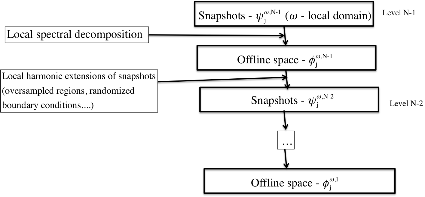
Figure 1: Illustration. The outline of the algorithm.

The success of numerical multiscale methods depends on adaptive simulations. The proposed method needs some adaptivity criteria to appropriately select the number of basis function in each level. We discuss adaptivity and present numerical results. The main idea of the adaptivity is to start at the coarsest level $H_{1}$ and identify the regions, which need additional multiscale basis functions. Then, within these regions, we identify smaller coarse regions (at the $H_{2}$ level), where one needs more basis functions. This procedure can be repeated until we reach the $H_{N-1}$ level. In this way, we identify the regions that need additional basis functions.

We would like to briefly draw a parallel between the proposed methods and hierarchical upscaling methods (such as re-iterated homogenization and their numerical counterparts). For this reason, we consider the flow problem

$$\text{div}(\kappa\nabla u)=f.$$

Our proposed approach shares a similarity with re-iterated numerical upscaling and can be regarded as a generalization (similar to the generalization of two-level GMsFEM and numerical upscaling, see [8]). In these upscaling approaches, the media properties are upscaled at each level and then used at the next level. Numerically, this can be considered in the following way. At the finest coarse-grid level, $H_{N-1}$, the effective properties, $\kappa^{*}_{N-1}$, are computed by solving the local problem subject to periodic or linear boundary conditions

$$\text{div}(\kappa\nabla\phi_{i})=0\ \text{in}\ K,$$

$\phi_{i}=x_{i}$ on $\partial K$, for each coarse-grid block $K$ at level $N-1$. Here, we use $K$ as a generic coarse block. Then, the effective properties are computed in each coarse block

$$\kappa_{K,N-1}^{*}={1\over|K|}\int_{K}\kappa\nabla\phi_{i}.$$

These coarse-grid conductivities are used to solve the local problem at the next level in the same way. The process is repeated until we reach the desired level $\kappa^{*}_{1}$, where the global problem is solved. As we have discussed in [8], the limited number of local solutions (which use $x_{i}$ boundary conditions) can be thought of as multiscale basis functions. Thus, the re-iterated homogenization or its numerical counterpart computes the next level of multiscale basis functions using the space spanned by the previous (finer) level multiscale basis functions. This concept is used in our approach with the exception that computing of multiscale basis functions is systematic and one can compute many basis functions. An important part in the re-iterated homogenization is that one uses the same linear boundary conditions at each level when solving local problems. Since the linear functions can be recovered at each level exactly, one does not need to change these boundary conditions. In our proposed method, we use all possible boundary conditions (randomization is used) spanned by multiscale basis functions of the previous (finer) coarse-grid level. The main advantage of the proposed method is that it can handle non-separable scales and high contrast by identifying an appropriate number of local problems to approximate the solution at each level.

In the paper, we consider several numerical examples. Our first set of numerical examples is for elliptic problems in heterogeneous domains. In these examples, we compare the results, when the multiscale basis functions are consrtucted using a multilevel approach and when the multiscale basis functions are constructed on the finest grid. Our numerical results show that one can achieve a similar accuracy. We present an adaptive startegy. The main idea is to first define the coarsest region, which needs an additional basis function. Then, within this region, we identify subregions, which need additional multiscale basis functions. The numerical results are presented for an adaptive method. Our second set of test examples includes problems in perofated domains. In these examples, the domain is heterogeneous. We present numerical results and show that one can approximate multiscale basis functions re-iteratively.

In summary, the paper is organized as follows. In Section 2, we present some preliminaries and notations. In Section 3, we present the main algorithm. Section 4 is devoted to numerical results. In Section 5, we discuss the computational cost of the proposed method. Finally, the paper ends with a conclusion in Section 6.

2 Preliminaries

In this section, we present an overview of the main concepts and introduce some notations. We consider the problem

$$\mathcal{L}u=f\ \text{in}\ D$$ (1)

where $\mathcal{L}$ is a differential operator, $D$ is a domain and $f$ is a given source term. We assume that the solution $u$ satisfies typical boundary conditions, such as the Dirichlet or the Neumann conditions on $\partial D$. In this paper, we consider two representative cases. In the first case, $\mathcal{L}u=\text{div}(\kappa\nabla u)$, where $\kappa$ is a heterogeneous coefficient with multiple scales and high contrast. In the second case, $\mathcal{L}u=\text{div}(\kappa\nabla u)$ and $D$ is a heterogeneous domain with holes (see Figure 6). The first case is a representative case for problems with heterogeneous coefficients and can easily be generalized to many other examples ([8]). The second case represents problems in perforated domains, which occur in many applications and can be generalized to other problems, e.g., Stokes flow in perforated domains. Moreover, the second example shows a need for snapshot solutions.

Next, we present the coarse and the fine grids. We assume that the final coarse-grid simulations will be performed on a grid $\mathcal{T}_{H}^{(1)}$ with a grid size $H_{1}$. Our objective is to construct multiscale basis functions on this grid. In the two-level setting of GMsFEM ([8]), the multiscale basis functions for the grid $\mathcal{T}_{H}^{(1)}$ are computed by solving cell problems for each coarse region of $\mathcal{T}_{H}^{(1)}$. The solutions to these cell problems are obtained numerically by using a discretization on a fine grid constructed within each coarse region. Solving these problems can be expensive due to scale disparity and it is therefore the purpose of this paper to investigate a re-iterated framework. In this regard, we assume that the grid $\mathcal{T}_{H}^{(1)}$ is subdivided into a sequence of finer grids $\mathcal{T}_{H}^{(l)}$ such that $\mathcal{T}_{H}^{(l-1)}\supset\mathcal{T}_{H}^{(l)}$, $l=2,...,N$, with corresponding grid sizes $H_{1}>H_{2}>\cdots>H_{N}=h$. Here, $h$ is the grid size of the finest grid and $N$ is the number of grids. Each coarse grid $\mathcal{T}_{H}^{(l)}$ consists of overlapping elements $\omega_{j,l}$, where $j$ is the index for the $j$-th vertex in the grid $\mathcal{T}_{H}^{(l)}$. For each $j$, we define $I_{j}$ as the set of all indices $m(j)$ such that

$$\omega_{j,l-1}\supset\omega_{m(j),l}.$$

More precisely, $\omega_{m(j),l}$ are the elements in the grid $\mathcal{T}_{H}^{(l)}$ that are contained in element $\omega_{j,l-1}\in\mathcal{T}_{H}^{(l-1)}$. We remark that the definition of $I_{j}$ is dependent on the level index $l$. Since the dependence of $I_{j}$ on $l$ will be clear in the context, we will omit this dependence to simplify our notations.

Our re-iterated GMsFEM will compute the basis functions for the grid $\mathcal{T}_{H}^{(1)}$ using the basis functions constructed for the grid $\mathcal{T}_{H}^{(2)}$, instead of a fine grid as in the two-level GMsFEM. More generally, we will compute multiscale basis functions for the grid $\mathcal{T}_{H}^{(l-1)}$ by using the multiscale basis functions for the grid $\mathcal{T}_{H}^{(l)}$, for $l=2,3,\cdots,N$, to approximate the cell problems. The main idea of our re-iterated approach is that the multiscale basis functions constructed for the level $l$ will give good approximations to the cell problems required in finding the basis functions for the level $(l-1)$. Next, we introduce the notations for the offline space and the snapshot space. Assume that the multiscale basis functions are already obtained for the level $l$. We call the space spanned by all these basis functions as the offline space, denoted by $V_{H,\text{off}}^{l}$. We notice that these basis functions are supported on the overlapping elements $\omega_{m,l}$. For each of these overlapping elements $\omega_{m.l}$, we denote the $j$-th basis functions by $\{\phi_{j}^{\omega_{m,l}}\}$. The local offline space $V_{H,\text{off}}^{\omega_{m,l}}$ is the space spanned by basis functions $\{\phi_{j}^{\omega_{m,l}}\}$. To construct the basis functions at the level $(l-1)$, we consider an element $\omega_{k,l-1}$. Following the idea of GMsFEM, we need a snapshot space $V_{H,\text{snap}}^{\omega_{k,l-1}}=\text{span}\{\psi_{j}^{\omega_{k,l-1}}\}$ defined on $\omega_{k,l-1}$. To construct the space $V_{H,\text{snap}}^{\omega_{k,l-1}}$, we will solve a cell problem on $\omega_{k,l-1}$ by using the multiscale basis functions constructed for the level $l$. Using the snapshot space and a suitable spectral problem, we can construct a set of offline basis $\{\phi_{j}^{\omega_{k,l-1}}\}$ by selecting the dominant modes defined using the spectral problem. The above procedure is repeated until the basis functions for the level $1$ are obtained. The precise constructions will be given in the next section.

Summary of notations

For the ease of reference, we summarize below the list of notations defined above.

• $\mathcal{T}_{H}^{(l)}$ is the coarse-grid configuration at level $l$, $\mathcal{T}_{H}^{(l-1)}\supset\mathcal{T}_{H}^{(l)}$, $l=2,...,N$.

• $H_{l}$ is the grid size of $\mathcal{T}_{H}^{(l)}$ ($H_{1}>H_{2}>...>H_{N}$).

• $\omega_{j,l}$ is the $j$-th coarse region at the coarse-grid level $l$.

• $I_{j}$ is the set of indices $m(j)$ such that $\omega_{j,l-1}\supset\omega_{m(j),l}$.

• $\{\psi_{j}^{\omega_{m,l}}\}$ is the set of snapshots at the coarse-grid level $l$, which are supported on $\omega_{m,l}$.

• $\{\phi_{j}^{\omega_{m,l}}\}$ is the set of offline basis at the coarse-grid level $l$, which are supported on $\omega_{m,l}$.

• $V_{H,\text{snap}}^{\omega_{m,l}}$ is the local snapshot space at the coarse-grid level $l$ for the subdomain $\omega_{m,l}$.

• $V_{H,\text{off}}^{\omega_{m,l}}$ is the local offline space at the coarse-grid level $l$ for the subdomain $\omega_{m,l}$.

• $V_{H,\text{snap}}^{l}$ is the global snapshot space at the coarse-grid level $l$.

• $V_{H,\text{off}}^{l}$ is the global offline space at the coarse-grid level $l$.

3 Re-iterated GMsFEM

In this section, we present the detail construction of the re-iterated GMsFEM. As we mentioned earlier that the algorithm is a systematic extension of the two-level approach with the main idea of using offline spaces of previous level (finer level) for construction of the snapshot space for the current level. The algorithm is illustrated in Figure 1, and we will explain next the full description of the algorithm.

The construction starts with a snapshot space for the level $(N-1)$ grid $\mathcal{T}_{H}^{(N-1)}$. To compute the snapshot vectors, we will solve local problems on an oversampled region with some appropriate randomized boundary conditions. In particular, for each oversampled region $\omega_{m,N-1}^{+}$, we solve

$$\mathcal{L}\psi_{j}^{\omega_{m,N-1}}=0,\quad\text{in }\omega_{m,N-1}^{+}$$ (2)

subject to boundary conditions $\psi_{j}^{\omega_{m,N-1}}=\mathcal{R}_{j}$, where $\mathcal{R}_{j}$ is a random function, which takes an independent random value at every boundary node. The equation (2) is solved on the finest grid $\mathcal{T}_{H}^{(N)}$ and can therefore be thought as a discrete equation defined on a fine grid $\mathcal{T}_{H}^{(N)}$. We notice that the snapshot space $V_{H,\text{snap}}^{\omega_{m,N-1}}$ is obtained by the spans of the restrictions of the above $\psi_{j}^{\omega_{m,N-1}}$ in $\omega_{m,N-1}$. We use the same notation for the solution of (2) and its restriction in $\omega_{m,N-1}$ to simplify the notations. We remark that the oversampled region $\omega_{m,N-1}^{+}$ is usually obtained by enlarging $\omega_{m,N-1}$ by several grid blocks of the finest mesh $\mathcal{T}_{H}^{(N)}$. Instead of the above construction of snapshot vectors, one can use other snapshot functions that use all boundary conditions or all fine grid functions (see [8]).

Next, we describe the iterated procedure. For a given level $l$, we assume that the snapshot space $V_{H,\text{snap}}^{l}$ is already determined. Recall that $V_{H,\text{snap}}^{\omega_{m,l}}$ is the local snapshot space corresponding to the coarse region $\omega_{m,l}$. We will first identify the offline space $V_{H,\text{off}}^{\omega_{m,l}}$ for this region. To do so, we will make use of two bilinear forms $a(\cdot,\cdot)$ and $s(\cdot,\cdot)$, and a suitable spectral problem defined in $V_{H,\text{snap}}^{\omega_{m,l}}$ to select some dominant modes. More precisely, we consider the spectral problem of finding $\lambda\in\mathbb{R}$ and $u\in V_{H,\text{snap}}^{\omega_{m,l}}$ such that

$$a(u,v)=\lambda s(u,v),\quad\forall v\in V_{H,\text{snap}}^{\omega_{m,l}}.$$

We then let $\lambda_{1}\leq\lambda_{2}\leq\cdots\leq\lambda_{K}$ be the eigenvalues and let $\widetilde{\phi}_{1},\widetilde{\phi}_{2},\cdots,\widetilde{\phi}_{K}$ be the corresponding eigenfunctions. The dominant modes are defined as the first few eigenfunctions. To construct the offline space $V_{H,\text{off}}^{\omega_{m,l}}$, we select the first few eigenfunctions and define the offline basis $\phi_{j}^{\omega_{m,l}}=\chi_{m}^{(l)}\widetilde{\phi}_{j}$, where $\{\chi_{m}^{(l)}\}$ is the partition of unity corresponding to the grid $\mathcal{T}_{H}^{(l)}$. The global offline space $V_{H,\text{off}}^{l}$ for the level $l$ is then defined as the span of all these basis functions. We remark that the choice of the bilinear forms $a(\cdot,\cdot)$ and $s(\cdot,\cdot)$ are based on the convergence analysis. For example, for elliptic equation considered in this paper, we will use

$$a(u,v) =\int_{\omega_{m,l}}\kappa\nabla u\cdot\nabla v,$$

$$s(u,v) =\int_{\omega_{m,l}}|\nabla\chi^{(l)}_{m}|^{2}\,u\,v.$$

The reader can see [8] for the spectral problems associated with other equations.

Once the offline space $V_{H,\text{off}}^{l}$ for the level $l$ is determined, we will construct the snapshot space for the level $(l-1)$. The main idea is that we will use the basis functions in $V_{H,\text{off}}^{l}$ to solve the cell problems in the level $(l-1)$. Consider a coarse region $\omega_{m,l-1}$ in the grid $\mathcal{T}_{H}^{(l-1)}$. We will need to construct the snapshot space $V_{H,\text{snap}}^{\omega_{m,l-1}}$, which is spanned by a set of basis functions $\psi_{j}^{\omega_{m,l-1}}$. Conceptually, we will solve

$$\mathcal{L}\psi_{j}^{\omega_{m,l-1}}=0,\quad\text{in }\omega_{m,l-1}.$$ (3)

To do so, we need to specify a discretization and a boundary condition. We recall that $I_{m}$ is the set of indices $k$ such that $\omega_{k,l}\subset\omega_{m,l-1}$. For the discretization of (3), we will assume that $\psi_{j}^{\omega_{m,l-1}}$ is a linear combination of all the offline basis $\phi_{j}^{\omega_{k,l}}\in V_{H,\text{off}}^{\omega_{k,l}}$ where $k\in I_{m}$. For the boundary condition for (3), we will take the restriction of $\phi_{j}^{\omega_{k,l}}$ on the boundary of $\omega_{m,l-1}$ with the condition that the restriction of non-zero. Thus, we have a set of linearly independent boundary conditions and these will generate the snapshot space $V_{H,\text{snap}}^{\omega_{m,l-1}}$. On the other hand, one can do the above computations on an oversampled region $\omega_{m,l-1}^{+}$, obtained by enlarging $\omega_{m,l-1}$ by few grid blocks in $\mathcal{T}_{H}^{(l)}$.

The above process is repeated until the coarsest grid, that is $l=1$, where multiscale basis functions are constructed and used for the numerical simulations. We summarize below the main steps of the algorithm.

The re-iterated GMsFEM

Initialization: Construct the snapshot space $V_{H,\text{snap}}^{\omega_{m,N-1}}$. Solve

$$\mathcal{L}\psi_{j}^{\omega_{m,N-1}}=0,\quad\text{in }\omega_{m,N-1}^{+}$$ (4)

subject to boundary conditions $\psi_{j}^{\omega_{m,N-1}}=\mathcal{R}_{j}$, where $\mathcal{R}_{j}$ is a random function. Then take the restriction of $\psi_{j}^{\omega_{m,N-1}}$ in $\omega_{m,N-1}$. We perform the above computations for each coarse region $\omega_{m,N-1}$ in the grid $\mathcal{T}_{H}^{(N-1)}$.

Iteration: For each $l=N-1,\cdots,1$, perform the following computations

• Construct the offline space $V_{H,\text{off}}^{\omega_{m,l}}$. Solve the spectral problem of finding $\lambda\in\mathbb{R}$ and $u\in V_{H,\text{snap}}^{\omega_{m,l}}$ such that

  $$a(u,v)=\lambda s(u,v),\quad\forall v\in V_{H,\text{snap}}^{\omega_{m,l}},$$

  and select the dominant modes.

• Construct the snapshot space $V_{H,\text{snap}}^{\omega_{m,l-1}}$. Solve the following equation

  $$\mathcal{L}\psi_{j}^{\omega_{m,l-1}}=0,\quad\text{in }\omega_{m,l-1}$$ (5)

  by using the offline spaces $V_{H,\text{off}}^{\omega_{k,l}}$, for all $k\in I_{m}$. The functions $\psi_{j}^{\omega_{m,l-1}}$ spans the space $V_{H,\text{snap}}^{\omega_{m,l-1}}$.

3.1 Adaptivity

In this part, we present an adaptive procedure for the re-iterated GMsFEM. The multilevel adaptive enrichment procedure is designed based on the two-level adaptive enrichment algorithm developed and analyzed in [14]. The main idea is to select coarse regions with larger errors, and then enrich the multiscale approximation space by adding basis functions in those selected coarse regions. There are two possibilities. First, we can use new multiscale basis functions at all pre-identified levels to update multiscale solution. Secondly, we can use new multiscale basis functions to update the basis functions at the coarsest level.

In the two-level setting, that is only the meshes $H_{1}$ and $H_{N}$ are used, we will select coarse regions in the mesh $H_{1}$ by computing a local residual. The local residual for the coarse region $\omega_{i,1}$ is defined as

$$R_{i}(v)=\int_{\omega_{i,1}}fv-\int_{\omega_{i,1}}\kappa\nabla u\cdot\nabla v,\quad\quad v\in V_{H,\text{off}}^{\omega_{i,N}}.$$ (6)

The norm of the residual is defined as

$$\|R_{i}\|=\sup_{v\in V_{H,\text{off}}^{\omega_{i,N}}}\frac{|R_{i}(v)|}{\|v\|_{\omega_{i,1}}},$$ (7)

where $\|v\|^{2}_{\omega_{i,1}}=\int_{\omega_{i,1}}\kappa|\nabla v|^{2}$. We remark that the residual (6) and its norm (7) are computed in the mesh $H_{N}=h$, which is the finest mesh. We define $\eta_{i}^{2}=\|R_{i}\|^{2}\lambda_{l_{i}+1}^{-1}$, and we enumerate the coarse regions in the mesh $H_{1}$ such that

$$\eta_{1}^{2}\leq\eta_{2}^{2}\leq\cdots,$$

where $l_{i}$ is the number of offline basis chosen for the region $\omega_{i,1}$. For a given real number $0<\theta<1$, we can choose the coarse regions so that

$$\theta\sum_{i=1}^{N}\eta_{i}^{2}<\sum_{i=1}^{k}\eta_{i}^{2}.$$ (8)

For those selected regions, we will add new offline basis functions in the approximation space. Secondly, we can use these basis functions to update the coarsest multiscale basis functions. The above process is terminated until a certain tolerance is reached.

Now we present the our adaptive enrichment procedure for several levels. The idea is that, to compute the residual and its norm, we will use the mesh in the next finer level. That is, for the residual in the mesh $H_{l}$, we will compute it using the mesh $H_{l+1}$. In particular, we define local residual for the coarse region $\omega_{i,l}$ as

$$R_{i,l}(v)=\int_{\omega_{i,l}}fv-\int_{\omega_{i,l}}\kappa\nabla u\cdot\nabla v,\quad\quad v\in V_{H,\text{off}}^{\omega_{i,l+1}}$$ (9)

with its norm defined by

$$\|R_{i}\|=\sup_{v\in V_{H,\text{off}}^{\omega_{i,l+1}}}\frac{|R_{i}(v)|}{\|v\|_{\omega_{i,l}}}$$ (10)

where $\|v\|^{2}_{\omega_{i,l}}=\int_{\omega_{i,l}}\kappa|\nabla v|^{2}$. This can provide a saving in computational time compared with the two-level approach (6)-(7).

For each iteration, we will determine coarse regions in the mesh $H_{1}$ using the criteria defined in (8). Then we will enrich the solution space by adding basis functions from $V_{H,\text{snap}}^{\omega_{i,1}}$. This is performed by adding the next eigenfunctions of the spectral problem. We remark that, by merely adding basis functions from the space $V_{H,\text{snap}}^{\omega_{i,1}}$, the solution may not be improved when a certain number of basis functions from $V_{H,\text{snap}}^{\omega_{i,1}}$ is included. One can observe this by the relative eigenvalue decay or the residual of the solution within coarse regions. To further enhance the accuracy of the solution, one need to include basis functions in the next level. In particular, for the selected coarse regions in the mesh $H_{1}$, we will compute the residual $R_{j,2}$ for the mesh $H_{2}$ for all sub coarse regions. Then, using the criteria in (8), we can select coarse regions for the mesh $H_{2}$ and add basis functions from the spaces $V_{H,\text{snap}}^{\omega_{j,2}}$. We can perform this computations until the relative decay of eigenvalue is small or the residual of the solution has little decay. After that, we will compute the residual in the next level, mesh $H_{3}$, and continue this process.

The second approach consists of using new enriched multiscale basis functions at level $2,3,...$ for re-computing multiscale basis functions at level $1$. In this approach, additional multiscale basis functions can be used for re-computing and adding new multiscale basis functions at level $1$. Alternatively, one can repeat the second approach for updating multiscale basis functions at level $3,...$ or use the first approach and select new multiscale basis functions at level $2,3,...$. In the paper, we will focus on the first approach.

Below is a flow chart of the algorithm in the three coarse-grid level setting ($N=3$). Assume the solution $u^{(n)}\in V^{(n)}$ at the $n$-th iteration is given. We will construct the solution $u^{(n+1)}$ by adding new basis functions in some selected coarse regions and some selected level $l$. To do so, we perform the following computations.

Step 1: Computing a solution:

• Compute a solution ${u}^{(n)}\in V^{(n)}$.

Step 2: Adding level 1 basis:

• Compute the residual norm $\|R_{i,1}\|$ in the coarse-grid level $1$ using $u^{(n)}$.

• Select coarse regions $\omega_{i,1}$, and add level-1 basis functions.

Step 3: Adding level 2 basis:

• Compute the residual norm $\|R_{i,2}\|$ in the regions selected in the previous step in the coarse-grid level $2$ using $u^{(n)}$.

• Select coarse regions $\omega_{i,2}$, and add level-2 basis functions.

Repeat Step 1 - 3 until the solution $u^{(n)}$ is accuracy enough.

Notice that the above adaptive process can be easily generalized to the multi-level case. Finally, we remark that one can also consider the goal-oriented adaptivity [12] or the residual-driven online adaptivity [10].

4 Numerical results

4.1 Numerical results for flow in heterogeneous media

In this section, we present a number of numerical examples to show the performance of the proposed method. The space domain $\Omega$ is taken as the unit square $[0,1]\times[0,1]$ and is divided into $10\times 10$ coarse blocks consisting of uniform squares in first coarse-grid level. Each coarse block is then divided into $4\times 4$ coarse blocks consisting of uniform squares in second level. Each second coarse block is divided into $10\times 10$ fine blocks consisting of uniform squares. That is, $\Omega$ is partitioned by $400\times 400$ square fine-grid blocks. The high-contrast permeability field $\kappa(x)$ is shown in Figure 3.

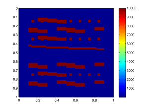
Figure 3: The permeability field $\kappa(x)$

To compare the accuracy, we will use the following error quantities:

$$e_{1}=\left(\frac{\|u_{H}-u_{h}\|^{2}_{L^{2}(\Omega)}}{\|u_{h}\|^{2}_{L^{2}(\Omega)}}\right)^{1/2},\qquad e_{2}=\left(\frac{\int_{\Omega}\kappa|\nabla(u_{H}-u_{h})|^{2}}{\int_{\Omega}\kappa|\nabla u_{h}|^{2}}\right)^{1/2}$$ (11)

$$e^{\text{snap}}_{1}=\left(\frac{\|u_{H}-u_{\text{snap}}\|^{2}_{L^{2}(\Omega)}}{\|u_{\text{snap}}\|^{2}_{L^{2}(\Omega)}}\right)^{1/2},\qquad e^{\text{snap}}_{2}=\left(\frac{\int_{\Omega}\kappa|\nabla(u_{H}-u_{\text{snap}})|^{2}}{\int_{\Omega}\kappa|\nabla u_{\text{snap}}|^{2}}\right)^{1/2}$$ (12)

where $u_{h}$ denotes the fine grid solution, $u_{\text{snap}}$ denotes the multiscale solution and $u_{H}$ denotes the multiscale solution.

First, we present result for multiscale method without adaptivity. We consider the source function $f=1$. In Table 1, we show the convergence history for using two coarse-grid level multiscale method (the coarsest grid versus the finest grid). We note that one can improve the results for two-level methods if mixed or hybridization is used [9]. Here, our goal is to get a comparable error to the two-level using a simplified basis construction. In Table 2, we show the convergence history for using three coarse-grid level multiscale method. For the same number of first coarse-grid level basis functions, we have two choices for the second level basis functions $10$ and $12$. We observe that the errors are similar to those using two-level approaches. This indicates that one can use more coarse-grid levels to inexpensively compute multiscale basis functions and achieve similar convergence.

$N_{1}$	$e_{2}$	$e_{1}$
1	47.15%	28.49%
2	26.40%	7.00%
4	21.01%	4.44%
6	18.90%	3.57%
8	17.25%	2.96%
10	16.23%	2.62%
12	15.37%	2.35%

Table 1: The result for two levels method. $N_{1}$ denotes the number of basis functions used per coarse block in first coarse-grid level.

$N_{1}$	$N_{2}$	$e_{2}$	$e_{1}$	$e^{\text{snap}}_{2}$	$e^{\text{snap}}_{1}$
2	10	26.06%	6.78%	20.78%	4.52%
4	10	21.02%	4.44%	14.00%	2.12%
6	10	19.10%	3.64%	11.02%	1.27%
8	10	17.99%	3.22%	9.02%	0.82%
10	10	17.61%	3.09%	8.42%	0.68%
12	10	17.37%	3.00%	8.01%	0.59%

$N_{1}$	$N_{2}$	$e_{2}$	$e_{1}$	$e^{\text{snap}}_{2}$	$e^{\text{snap}}_{1}$
2	12	26.05%	6.78%	20.77%	4.52%
4	12	21.00%	4.44%	14.00%	2.12%
6	12	19.12%	3.65%	11.07%	1.28%
8	12	17.95%	3.20%	9.00%	0.81%
10	12	17.54%	3.06%	8.30%	0.65%
12	12	17.29%	2.97%	7.86%	0.56%

Table 2: The result for three coarse-grid level method. $N_{1}$ denotes the number of basis functions used per coarse block in first coarse-grid level. $N_{2}$ denotes the number of basis functions used per coarse block in second coarse-grid level.

Adaptivity

In this section, we present the numerical result for the adaptive multiscale method. As we mentioned that one can adaptively update the number of multiscale basis functions. This can reduce the degrees of freedom needed to represent local basis functions. In our numerical examples, we consider a different source function, $f$, which is shown in Figure 4.

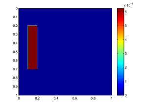
Figure 4: source $f$

In Table 3 and Figure 5, we show the results for enriching basis in different coarse-grid levels. As we observe from this figure that one can lower the error using adaptive methods. In particular, in the first table in Table 3, we present the errors when we adaptively enrich the basis functions in both level 1 and level 2. We observe that this gives much better results when basis functions are only enriched in one level (results are shown in the other two tables). More clearly, one can see in Figure 5 a comparison among these 3 cases, and we observe that enriching basis in both levels gives the best results.

$DOF_{1}$	$DOF_{2}$	$e^{\text{snap}}_{2}$	$e^{\text{snap}}_{1}$
162	0	34.12%	7.57%
188	74	18.82%	4.18%
247	262	12.63%	2.17%
326	545	9.51%	1.28%
403	906	7.06%	0.74%
480	1329	5.57%	0.46%

$DOF_{1}$	$DOF_{2}$	$e^{\text{snap}}_{2}$	$e^{\text{snap}}_{1}$
162	0	34.12%	7.57%
185	0	21.18%	4.90%
242	0	17.23%	3.62%
320	0	15.41%	3.03%
405	0	14.34%	2.69%
493	0	13.61%	2.46%

$DOF_{1}$	$DOF_{2}$	$e^{\text{snap}}_{2}$	$e^{\text{snap}}_{1}$
162	0	34.12%	7.57%
162	57	28.22%	6.08%
162	125	24.45%	5.32%
162	284	17.20%	3.66%
162	552	13.78%	2.37%
162	894	10.92%	1.50%

Table 3: Comparison for enriching basis in different coarse-grid levels. $DOF_{1}$ denotes the number of basis funtions used in the first coarse-grid level. $DOF_{2}$ denotes the number of basis funtions used in the second coarse-grid level.

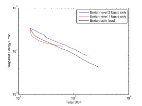
Figure 5: log-log scale error comparison

4.2 Numerical results for perforated domain

In this section, we consider a second example, a problem in perforated domain. We have studied these examples for two-level approaches in our earlier works [15, 13]. We present the numerical results for four coarse-grid levels. The computational domain $\Omega$ is taken to be $[0,1]\times[0,0.8]$ with $230$ random perforations. We solve elliptic equaion with source function $f=1$ with zero Dirichlet boundary conditions on perforations and global boundary. Fine-scale mesh contains $164835$ vertices and $326048$ triangular cells. We will use several numbers of the nested (embedded) coarse grids. Size of the fine-scale system is $DOF_{f}=164835$.

First, we consider a case with a homogeneous background, i.e., the permeability outside perforations is $1$. We divide the fine grid into several number of coarse-grid levels and present numerical results for the following configurations:

• Using 2 Levels = $L1+L4$;

• Using 3 Levels = $L1+L2+L4$;

• Using 4 Levels = $L1+L2+L3+L4$.

Here, we use

• Level 1: 30 vertices and 40 cells (4x5);

• Level 2: 357 vertices and 640 cells (4x4 for each cell from Level 1);

• Level 3: 5265 vertices and 10240 cells (4x4 for each cell from Level 2);

• Level 4 (fine-grid): 164835 vertices and 326048 cells.

At each level, we use a triangular grid. For the illustration of the mesh levels, we refer to Figure 6. Two coarse-grid level $L1+L4$ refers to the computations, where the fine grid $L4$ is used to compute multiscale basis functions $L1$. Three coarse-grid level $L1+L2+L4$ refers to the computation, where $L2+L4$ is used to compute multiscale basis functions. Four coarse-grid level $L1+L2+L3+L4$ refers to the computations, where $L2+L3+L4$ is used to compute multiscale basis functions.

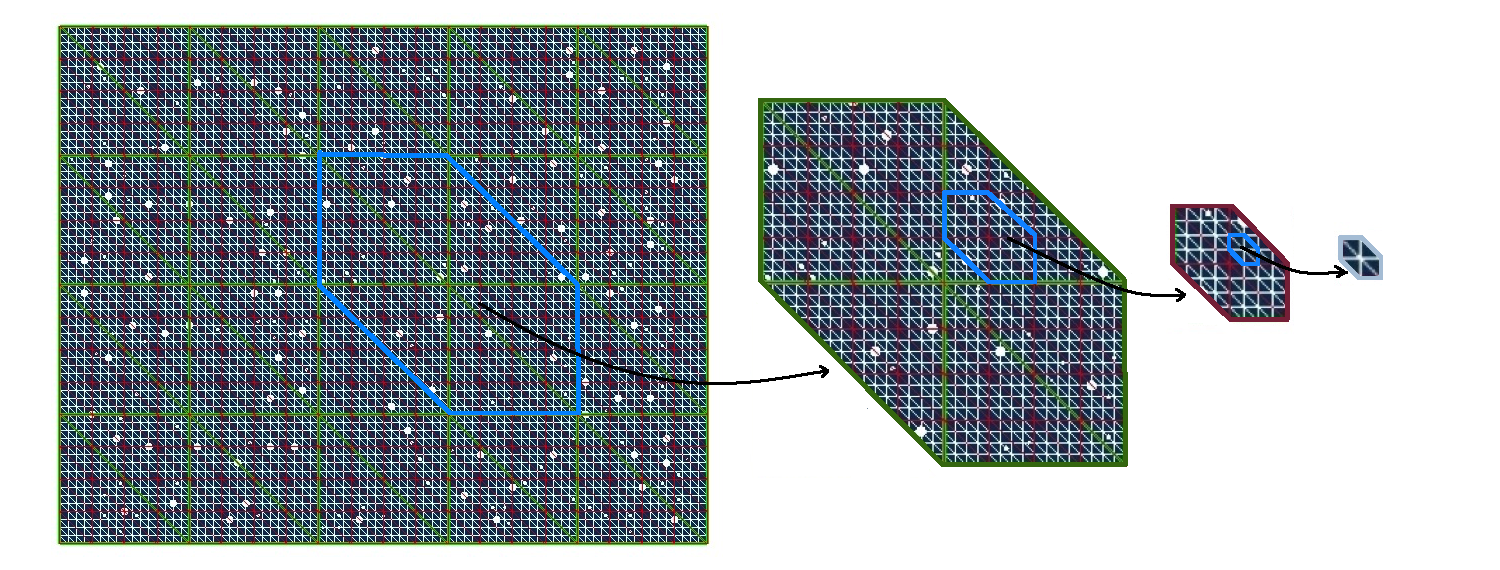
Figure 6: Computational meshes for perforated domain (230 random circle perforations) with 4 Levels. Level 1: green. Level 2: red. Level 3: white. Level 4 (fine grid): blue. Fine grid contains 164835 vertices and 326048 cells.

In Figure 7, we show the numerical solution of the elliptic problem using $4$ coarse-grid level multiscale method using different number of the multiscale basis at first coarsest level. In this case, we select $8$ basis functions at the coarsest level ($N_{1}=8$) and also use $8$ basis functions at each finer coarse-grid level for computing the multiscale basis functions. The numerical results for various number of multiscale basis functions at the coarsest level are presented in Table 4 (see also Figure 8 for illustration). In this table, we compare the results obtained using two level approach, where multiscale basis functions are computed on the fine grid to the results, when multiscale basis functions are computed using $N_{2}=8$ and $N_{2}=N_{3}=8$, which use very few degrees of freedom to approximate the basis functions. As we observe from this table that the errors are very similar, i.e., one can use approximations for computing multiscale basis functions. We observe similar results when fewer multiscale basis functions are chosen at finer coarse-grid levels. In Table 5, we present numerical results by varying the number of multiscale basis functions at finer levels. In particular, $N_{2}$ and $N_{3}$ are varied. Numerical results show that one can achieve a similar accuracy. We depict the numerical errors in Figure 9.

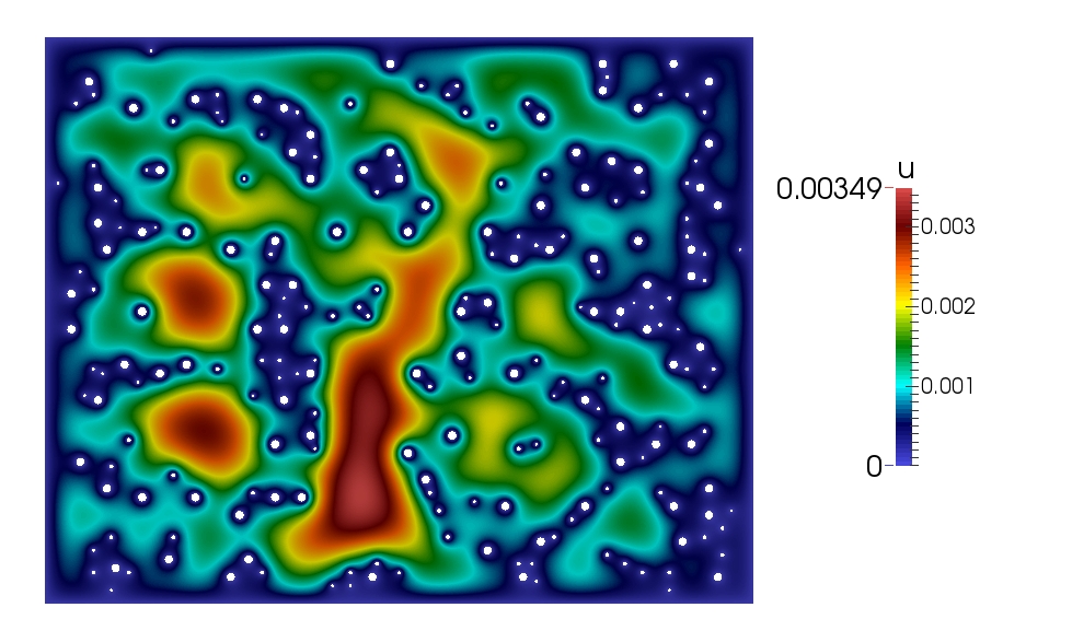
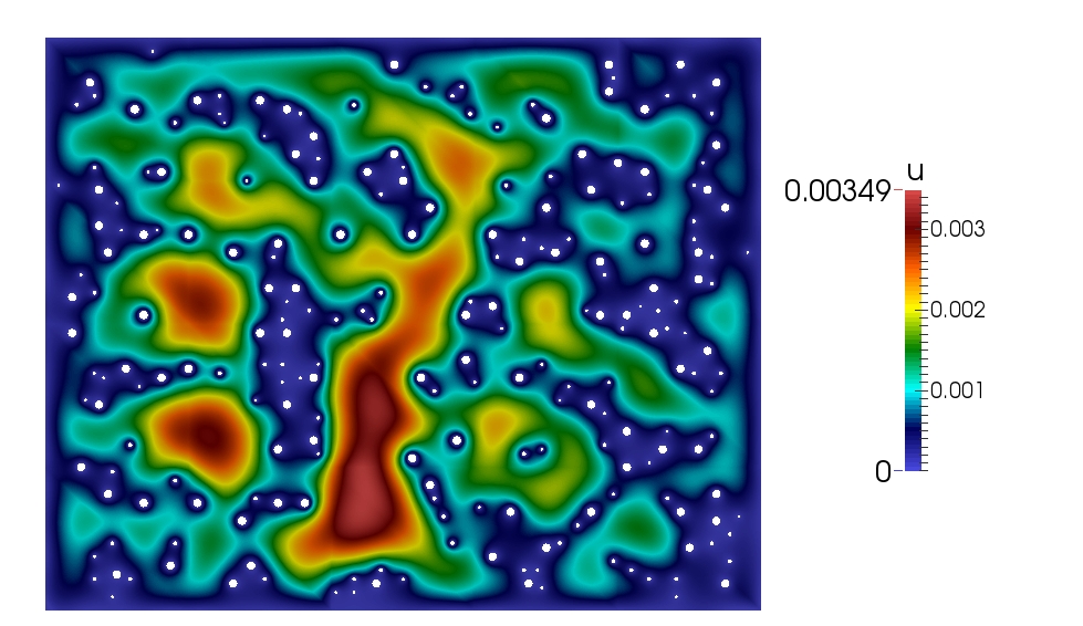
Figure 7: Fine-scale solution (left) and coarse-scale solution (right) using $8$ multiscale basis functions at level $L1$ ($N_{1}=8$) and $8$ basis functions for each other levels $N_{2}=N_{3}=8$.

		Using 2 Levels		Using 3 Levels		Using 4 Levels
				($N_{2}=8$)		($N_{2}=N_{3}=8$)
$N_{1}$	$DOF$	$e_{2}$	$e_{a}$	$e_{2}$	$e_{a}$	$e_{2}$	$e_{a}$
1	30	59.69	74.52	59.74	74.64	59.86	74.77
2	60	42.78	59.37	42.87	59.63	42.98	59.83
4	120	24.24	41.88	24.35	42.38	24.44	42.69
6	180	12.64	26.99	12.72	27.84	12.81	28.35
8	240	7.98	20.98	8.07	22.12	8.16	22.76
12	360	4.93	15.54	5.06	17.13	5.15	17.95
16	480	3.40	12.12	3.59	14.19	3.68	15.18

Table 4: Relative $L_{2}$ and energy errors for perforated domain using different number of coarse-grid levels (2, 3 and 4). $DOF_{f}=164835$.

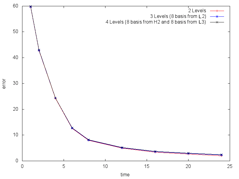
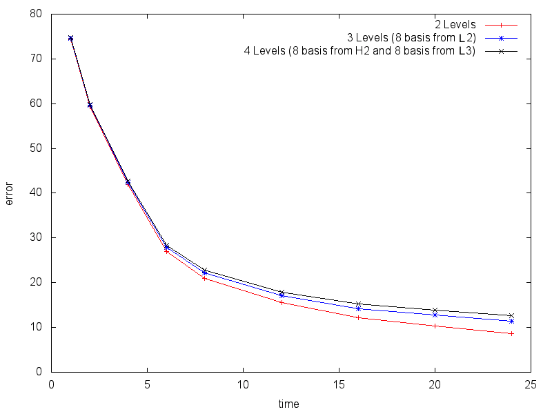
Figure 8: Illustration of Table 4. Relative $L_{2}$( left) and energy (right) errors for perforated domain.

	$N_{3}=4$		$N_{3}=8$		$N_{3}=16$
$N_{1}$	$e_{2}$	$e_{a}$	$e_{2}$	$e_{a}$	$e_{2}$	$e_{a}$
$N_{2}=4$
1	60.27	75.40	60.21	75.20	60.14	75.07
2	43.68	61.14	43.42	60.58	43.36	60.38
4	25.13	44.83	24.93	43.92	24.84	43.53
6	13.84	32.06	13.26	30.23	13.18	29.60
8	9.28	27.30	8.619	25.08	8.49	24.27
12	6.56	23.67	5.69	20.94	5.52	19.93
16	5.26	21.63	4.22	18.55	3.95	17.30
$N_{2}=8$
1	59.93	75.00	59.86	74.77	59.80	74.66
2	43.24	60.40	42.98	59.83	42.93	59.64
4	24.61	43.65	24.44	42.69	24.37	42.31
6	13.33	30.32	12.81	28.35	12.76	27.72
8	8.74	25.22	8.16	22.76	8.08	21.93
12	5.90	21.12	5.15	17.95	5.03	16.82
16	4.61	18.89	3.68	15.18	3.49	13.73

Table 5: Relative $L_{2}$ and energy errors for perforated domain using 4 coarse-grid levels and different number of $N_{2}$ and $N_{3}$. $DOF_{f}=164835$.

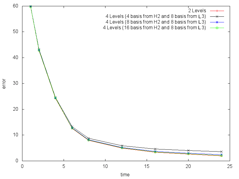
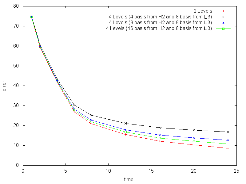
Figure 9: Illustration of Table 5. Relative $L_{2}$ (left) and energy (right) errors for perforated domain.

We have observed similar results when using a heterogeneous background as shown in Figure 10 with three-level coarse grids.

• Level 1: 99 vertices and 160 cells (8 to 10);

• Level 2: 1353 vertices and 2560 cells (4x4 for each cell from Level 1);

• Level 3 (fine-grid): 164835 vertices and 326048 cells.

At each level we have triangular grid. In Figure 11, we depict the fine-scale solution and the solution obtained using $8$ multiscale basis functions at the coarsest level $N_{1}=8$ and $N_{2}=8$. In Table 6, we present the errors by varying $N_{1}$, the number of basis functions at the coarsest level. As we observe that approximation of multiscale basis functions gives similar errors as two-level approaches. In this table, we also compare to the results obtained for homogeneous background. As we observe that the errors for the homogeneous background is better compared to those for the heterogeneous background.

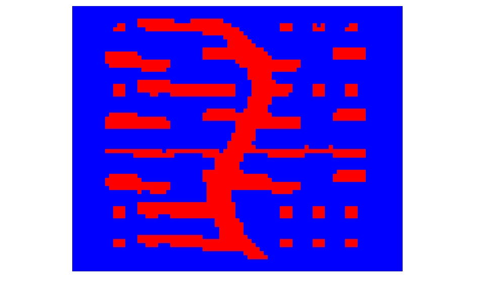
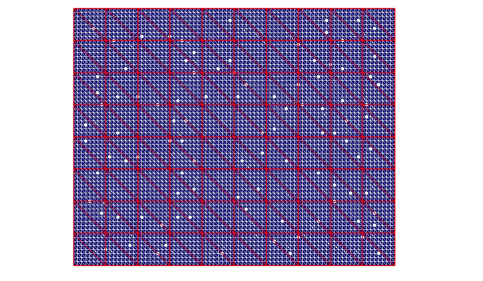
Figure 10: Heterogeneous backround (left) and computational grid (right) for perforated domain (230 random circle perforations) with three coarse-grid levels. Coarse-grid level 1: red. Coarse-grid level 2: white. Coarse-grid level 3 (fine grid): blue. Fine grid contains 164835 vertices and 326048 cells. In the left picture: $k=1$ in red domain and $k=1000$ in the blue domain.

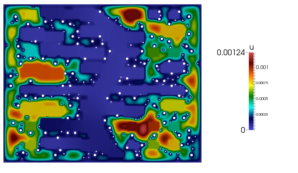
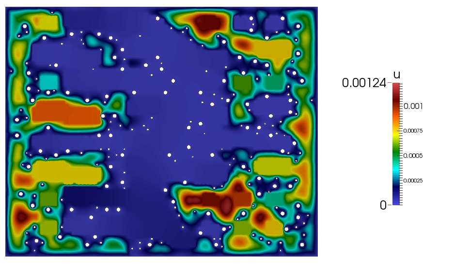
Figure 11: Fine-scale solution (top) and coarse-scale solution using $8$ multiscale basis functions at the coarsest level and $8$ basis functions at the finer levels to compute these multiscale basis functions. $L_{2}$ error is $0.87$%.

		Using 2 Levels		Using 3 Levels
				($N_{2}=8$)
$N_{1}$	$DOF$	$e_{2}$	$e_{a}$	$e_{2}$	$e_{a}$
Heterogeneous backround
1	30	79.56	94.80	79.61	94.81
2	60	55.64	84.28	55.75	84.36
4	120	22.36	57.57	22.55	57.92
6	180	1.781	42.42	2.11	43.00
8	240	1.31	33.98	1.69	34.77
12	360	0.67	23.96	1.05	25.15
16	480	0.42	17.98	0.87	19.71
Homogeneous backround
1	30	31.59	54.86	31.86	55.23
2	60	17.02	37.03	17.26	37.66
4	120	7.68	22.70	7.86	23.78
6	180	4.18	15.76	4.35	17.31
8	240	2.83	12.29	3.01	14.29
12	360	1.42	7.95	1.66	10.84
16	480	0.89	5.96	1.18	9.48

Table 6: Relative $L_{2}$ and energy errors for perforated domain with heterogeneous and homogeneous backrounds for different number of coarse-grid levels (2 and 3) $DOF_{f}=164835$.

5 Computational cost

One of our aims is to compute multiscale basis functions at the coarsest level for problems when disparity of scales does not allow such computations. In this sense, our approach has a similar concept as re-iterated homogenization with the aim of computing a reduced-order model. For this reason, our coarsening factors are usually very large. Besides allowing basis computations in extreme disparate scale cases, re-iterated approach can provide computational savings. Below, we discuss the computational savings.

Let $C_{i}$ be the coarsening number for level $i$ with the total number of fine grids $N=\Pi_{i}C_{i}$. Let $L:\mathbb{N}\rightarrow\mathbb{N}$ be the operation counting operator for the solver of the local snapshot problem where $L(N)$ is the number of operation for solving a local problem with size $N$. Furthermore, let $P:\mathbb{N}\times\mathbb{N}\rightarrow\mathbb{N}$ be the operation counting operator for the solver of the local eigenvalue problem where $P(a,b)$ is the number of operation for finding the first $b$ eigenvector with the local eigenvalue problem size $a$.

The operation number for constructing two level multiscale basis, $O_{2}$, (ignoring the time for forming matrix and gridding) is

$$O_{2}=O(C_{1}r_{1}L(M_{1}\Pi_{i>1}C_{i})+P(r_{1},\lambda_{1})),$$

where $M_{1}$ depends on the coarse grid structure and the oversampling size, $r_{1}$ depends on the number of random basis solved for each node and $\lambda_{1}$ depends on the number of basis chosen for each node. The operation count for constructing re-iterated multiscale basis functions, $O_{2}$, (ignoring the time for forming matrix and griding) is

$$O_{M}=O\left(\sum_{j=1}^{M-1}\left((\Pi_{i\leq j}C_{i})r_{i}L(\lambda_{i+1}M_{i}C_{i+1})+P(r_{i},\lambda_{i})\right)\right).$$

We assume $M_{i}C_{i+1}>r_{i}>\lambda_{i}$, $P(r_{i},\lambda_{i})=O(\lambda_{i}r_{i}^{\beta})$, and $L(N)=O(N^{\alpha})$ and $\alpha\geq\beta$. We remark that the operator, $L$, is dependent on the contrast of the medium parameter. For a high contrast medium, we expect to have a better performance of the local solver for re-iterated case. Then

$$O_{2} =O(C_{1}r_{1}L(M_{1}\Pi_{i>1}C_{i}))$$

$$O_{M} =O\left(\sum_{j=1}^{I-1}(\Pi_{i\leq j}C_{i})r_{i}L(\lambda_{i+1}M_{i}C_{i+1})\right).$$

We further assume $r_{i}=r,\;M_{i}=M,\;C_{i}=C\;\forall i\geq 1$ and $\lambda_{i}=\lambda\;\forall i\leq M-1$,

$$O_{M} =O\left(rM^{\alpha}\left(\sum_{j=1}^{M-2}\lambda^{\alpha}(\Pi_{i\leq j}C)C^{\alpha})+C^{M-1}C^{\alpha}\right)\right)$$

$$=O\left(rM^{\alpha}C^{\alpha}C\left(\lambda^{\alpha}\cfrac{C^{M-2}-1}{C-1}+C^{M-2}\right)\right)$$

and

$$O_{2}=O\left(rM^{\alpha}CC^{(M-1)\alpha}\right).$$

If $C>\lambda^{\alpha},$ we have

$$O_{2} =O\left(\cfrac{C^{(M-2)\alpha}}{C^{M-2}}O_{M}\right)$$

$$=O\left(C^{(M-2)(\alpha-1)}O_{M}\right).$$

Thus, if the coarsening factor is large and fewer basis functions are selected (cf., re-iterated homogenization, when the number of basis functions is very low), the re-iterated construction will provide a computational advantage. One of additional main advantage will be due to adaptivity, where only a few basis functions are needed in many regions.

6 Conclusions

In applications, the coarse computational grid may have very high resolution so that one can not afford local simulations to extract important modes within GMsFEM. In these cases, approximate calculations are needed. This paper presents an extension of two-level GMsFEM by re-iteration (similar to homogenization) to approximate multiscale basis functions on the coarsest level inexpensively. Following the general concept of the GMsFEM, we define snapshots at each level, which consist of all possible basis functions at the previous (finer) levels. This is a natural extension and shares some similarities with re-iterated homogenization methods, where the homogenization is carried out at separate levels and used in the next coarse level. We present an adaptive procedure and demonstrate numerical results for two applications.

Acknowledgements. EC’s research was in part supported by Hong Kong RGC General Research Fund Project No. 400813. MV’s work is partially supported by Russian Science Foundation Grant RS 15-11-10024 and RFBR 15-31-20856.

References

- [1] A. Abdulle and B. Engquist. Finite element heterogeneous multiscale methods with near optimal computational complexity. SIAM J. Multiscale Modeling and Simulation, 6(4):1059–1084, 2007.
- [2] G. Allaire and R. Brizzi. A multiscale finite element method for numerical homogenization. SIAM J. Multiscale Modeling and Simulation, 4(3):790–812, 2005.
- [3] A. Bensoussan, J. L. Lions, and G. Papanicolaou. Asymptotic analysis for periodic structures, volume 5 of Studies in Mathematics and Its Applications. North-Holland, 1978.
- [4] A. Brandt. Multiscale computational methods: research activities. In T. Chan and Z.-C. Shi, editors, Proc. 1991 Hang Zhou International Conf. on Scientific Computation, pages 1–7, Singapore, 1992. World Scientific Publishing Co.
- [5] A. Brandt. Multiscale scientic computation: Six year summary. Gauss Center Report, pages WI/GC–12, 1999.
- [6] Donald L Brown, Yalchin Efendiev, and Viet Ha Hoang. An efficient hierarchical multiscale finite element method for stokes equations in slowly varying media. Multiscale Modeling & Simulation, 11(1):30–58, 2013.
- [7] Victor M Calo, Eric T Chung, Yalchin Efendiev, and Wing Tat Leung. Multiscale stabilization for convection-dominated diffusion in heterogeneous media. Computer Methods in Applied Mechanics and Engineering, 304:359–377, 2016.
- [8] E. Chung, Y. Efendiev, and T. Hou. Adaptive multiscale model reduction with generalized multiscale finite element methods. Journal of Computational Physics. 10.1016/j.jcp.2016.04.054.
- [9] Eric Chung, Yalchin Efendiev, and Thomas Y Hou. Adaptive multiscale model reduction with generalized multiscale finite element methods. Journal of Computational Physics, 2016.
- [10] Eric T Chung, Yalchin Efendiev, and Wing Tat Leung. Residual-driven online generalized multiscale finite element methods. Journal of Computational Physics, 302:176–190, 2015.
- [11] Eric T Chung and Wing Tat Leung. A sub-grid structure enhanced discontinuous galerkin method for multiscale diffusion and convection-diffusion problems. Communications in Computational Physics, 14(02):370–392, 2013.
- [12] Eric T Chung, Wing Tat Leung, and Sara Pollock. Goal-oriented adaptivity for gmsfem. Journal of Computational and Applied Mathematics, 296:625–637, 2016.
- [13] Eric T Chung, Wing Tat Leung, and Maria Vasilyeva. Mixed gmsfem for second order elliptic problem in perforated domains. Journal of Computational and Applied Mathematics, 304:84–99, 2016.
- [14] ET Chung, Y Efendiev, and G Li. An adaptive GMsFEM for high-contrast flow problems. Journal of Computational Physics, 273:54–76, 2014.
- [15] ET Chung, Y Efendiev, G Li, and M Vasilyeva. Generalized multiscale finite element methods for problems in perforated heterogeneous domains. arXiv preprint arXiv:1501.03536, 2015.
- [16] Doina Cioranescu, Alain Damlamian, and Georges Griso. Periodic unfolding and homogenization. Comptes Rendus Mathematique, 335(1):99–104, 2002.
- [17] L.J. Durlofsky. Numerical calculation of equivalent grid block permeability tensors for heterogeneous porous media. Water Resour. Res., 27:699–708, 1991.
- [18] W. E and B. Engquist. Heterogeneous multiscale methods. Comm. Math. Sci., 1(1):87–132, 2003.
- [19] Jens Eberhard, Sabine Attinger, and Gabriel Wittum. Coarse graining for upscaling of flow in heterogeneous porous media. Multiscale Modeling & Simulation, 2(2):269–301, 2004.
- [20] Y. Efendiev, J. Galvis, and T. Hou. Generalized multiscale finite element methods. Journal of Computational Physics, 251:116–135, 2013.
- [21] Y. Efendiev, J. Galvis, and P.S. Vassilevski. Multiscale Spectral AMGe Solvers for High-Contrast Flow Problems. Submitted.
- [22] Y. Efendiev, J. Galvis, and X.H. Wu. Multiscale finite element methods for high-contrast problems using local spectral basis functions. Journal of Computational Physics, 230:937–955, 2011.
- [23] Y. Efendiev and T. Hou. Multiscale Finite Element Methods: Theory and Applications. Springer, 2009.
- [24] Y. Efendiev, T. Hou, and X.H. Wu. Convergence of a nonconforming multiscale finite element method. SIAM J. Numer. Anal., 37:888–910, 2000.
- [25] Yalchin Efendiev, Eric Chung, Guanglian Li, and Tat Leung. Sparse generalized multiscale finite element methods and their applications. International Journal for Multiscale Computational Engineering, (1):1–23, 2016.
- [26] Yalchin Efendiev, Juan Galvis, Guanglian Li, and Michael Presho. Generalized multiscale finite element methods: Oversampling strategies. International Journal for Multiscale Computational Engineering, 12(6), 2014.
- [27] Rong Fan, Zheng Yuan, and Jacob Fish. Adaptive two-scale nonlinear homogenization. International Journal for Computational Methods in Engineering Science and Mechanics, 11(1):27–36, 2010.
- [28] Jacob Fish. Practical multiscaling. John Wiley & Sons, 2013.
- [29] Jacob Fish, Tao Jiang, and Zheng Yuan. A staggered nonlocal multiscale model for a heterogeneous medium. International Journal for Numerical Methods in Engineering, 91(2):142–157, 2012.
- [30] Jacob Fish and Sergey Kuznetsov. From homogenization to generalized continua. International Journal for Computational Methods in Engineering Science and Mechanics, 13(2):77–87, 2012.
- [31] Jacob Fish, A Suvorov, and Vladimir Belsky. Hierarchical composite grid method for global-local analysis of laminated composite shells. Applied Numerical Mathematics, 23(2):241–258, 1997.
- [32] Jacob Fish and Amir Wagiman. Multiscale finite element method for a locally nonperiodic heterogeneous medium. Computational Mechanics, 12(3):164–180, 1993.
- [33] Leo Franca, JVA Ramalho, and F Valentin. Multiscale and residual-free bubble functions for reaction-advection-diffusion problems. International Journal for Multiscale Computational Engineering, 3(3), 2005.
- [34] Longfei Gao, Xiaosi Tan, and Eric T Chung. Application of the generalized multiscale finite element method in parameter-dependent pde simulations with a variable-separation technique. Journal of Computational and Applied Mathematics, 300:183–191, 2016.
- [35] Viet Ha Hoang and Christoph Schwab. High-dimensional finite elements for elliptic problems with multiple scales. Multiscale Modeling & Simulation, 3(1):168–194, 2005.
- [36] T. Hou and X.H. Wu. A multiscale finite element method for elliptic problems in composite materials and porous media. J. Comput. Phys., 134:169–189, 1997.
- [37] V. Jikov, S. Kozlov, and O. Oleinik. Homogenization of differential operators and integral functionals. Springer-Verlag, Translated from Russian, 1994.
- [38] Aiqin Li, Renge Li, and Jacob Fish. Generalized mathematical homogenization: from theory to practice. Computer Methods in Applied Mechanics and Engineering, 197(41):3225–3248, 2008.
- [39] JL Lions, D Lukkassen, LE Persson, and P Wall. Reiterated homogenization of nonlinear monotone operators. Chinese Annals of Mathematics, 22(01):1–12, 2001.
- [40] Konstantin Lipnikov, J David Moulton, and Daniil Svyatskiy. A multilevel multiscale mimetic (m 3) method for two-phase flows in porous media. Journal of Computational Physics, 227(14):6727–6753, 2008.
- [41] Konstantin Lipnikov, J David Moulton, and Daniil Svyatskiy. Adaptive strategies in the multilevel multiscale mimetic (m 3) method for two-phase flows in porous media. Multiscale Modeling & Simulation, 9(3):991–1016, 2011.
- [42] Scott P MacLachlan and J David Moulton. Multilevel upscaling through variational coarsening. Water resources research, 42(2), 2006.
- [43] Anthony Nouy and Pierre Ladevèze. Multiscale computational strategy with time and space homogenization: a radial-type approximation technique for solving microproblems. International Journal for Multiscale Computational Engineering, 2(4), 2004.
- [44] J Tinsley Oden, Kumar Vemaganti, and Nicolas Moës. Hierarchical modeling of heterogeneous solids. Computer Methods in Applied Mechanics and Engineering, 172(1):3–25, 1999.
- [45] M. Ohlberger. A posteriori error estimates for the heterogeneous multiscale finite element method for elliptic homogenization problems. SIAM J. Multiscale Modeling and Simulation, 4(1):88–114, 2005.
- [46] Christoph Schwab. High dimensional finite elements for elliptic problems with multiple scales and stochastic data. arXiv preprint math/0305007, 2003.
- [47] Panayot S. Vassilevski. Multilevel Block Factorization Preconditioners Matrix-based Analysis and Algorithms for Solving Finite Element Equations. Springer, New York, 2008.
- [48] P.S. Vassilevski. Coarse Spaces by Algebraic Multigrid: Multigrid Convergence and Upscaling Error Estimates. Advances in Adaptive Data Analysis, 3(1-2):229–249, 2011.
- [49] X.H. Wu, Y. Efendiev, and T.Y. Hou. Analysis of upscaling absolute permeability. Discrete and Continuous Dynamical Systems, Series B., 2:158–204, 2002.
- [50] Zheng Yuan and Jacob Fish. Hierarchical model reduction at multiple scales. International journal for numerical methods in engineering, 79(3):314–339, 2009.