The vacant set of two-dimensional critical random interlacement is infinite

Abstract

For the model of two-dimensional random interlacements in the critical regime (i.e., $\alpha=1$), we prove that the vacant set is a.s. infinite, thus solving an open problem from [8]. Also, we prove that the entrance measure of simple random walk on annular domains has certain regularity properties; this result is useful when dealing with soft local times for excursion processes.
Keywords: random interlacements, vacant set, critical regime, simple random walk, Doob’s $h$-transform, annular domain
AMS 2010 subject classifications: Primary 60K35. Secondary 60G50, 82C41.

${}^{~{}1}$Université Paris Diderot – Paris 7, Mathématiques, case 7012, F–75205 Paris Cedex 13, France
e-mail: comets@math.univ-paris-diderot.fr

${}^{~{}2}$Department of Statistics, Institute of Mathematics, Statistics and Scientific Computation, University of Campinas – UNICAMP, rua Sérgio Buarque de Holanda 651, 13083–859, Campinas SP, Brazil
e-mail: popov@ime.unicamp.br

1 Introduction and results

The model of random interlacements, recently introduced by Sznitman [17], has proved its usefulness for studying fine properties of traces left by simple random walks on graphs. The “classical” random interlacements is a Poissonian soup of (transient) simple random walks’ trajectories in ${\mathbb{Z}}^{d}$, $d\geq 3$; we refer to recent books [5, 12]. Then, the model of two-dimensional random interlacements was introduced in [8]. Observe that, in two dimensions, even a single trajectory of a simple random walk is space-filling. Therefore, to define the process in a meaningful way, one uses the SRW’s trajectories conditioned on never hitting the origin, see the details below. We observe also that the use of conditioned trajectories to build the interlacements goes back to Sznitman [19], see the definition of “tilted random interlacements” there. Then, it is known (Theorem 2.6 of [8]) that, for a random walk on a large torus conditioned on not hitting the origin up to some time proportional to the mean cover time, the law of the vacant set around the origin is close to that of random interlacements at the corresponding level. This means that, similarly to higher-dimensional case, two-dimensional random interlacements have strong connections to random walks on discrete tori.

Now, let us recall the formal construction of (discrete) two-dimensional random interlacements.

In the following, $\|\cdot\|$ denotes the Euclidean norm in ${\mathbb{R}}^{2}$ or ${\mathbb{Z}}^{2}$, and ${\mathsf{B}}(x,r)=\{y:\|x-y\|\leq r\}$ is the (closed) ball of radius $r$ centered in $x$. We write $f(n)=O(g(n))$ as $n\to\infty$ when, for some constant $M>0$, $|f(n)|\leq M|g(n)|$ for all large enough $n$; $f(n)=o(g(n))$ means that $\lim_{n\to\infty}\frac{f(n)}{g(n)}=0$. Also, we write $f(n)\sim g(n)$ when $\lim_{n\to\infty}\frac{f(n)}{g(n)}=1$. In fact, the same symbol is also used for neighboring sites: for $x,y\in{\mathbb{Z}}^{d}$ we write $x\sim y$ if $\|x-y\|=1$, that is, $x$ and $y$ are neighbors. Hopefully, this creates no confusion since the meaning of “$\sim$” will always be clear from the context.

Let $(S_{n},n\geq 0)$ be two-dimensional simple random walk. Write ${\mathbb{P}}_{x}$ for the law of the walk started from $x$ and ${\mathbb{E}}_{x}$ for the corresponding expectation. Let

$$\tau_{0}(A) =\inf\{k\geq 0:S_{k}\in A\},$$ (1)

$$\tau_{1}(A) =\inf\{k\geq 1:S_{k}\in A\}$$ (2)

be the entrance and the hitting time of the set $A$ by simple random walk $S$ (we use the convention $\inf\emptyset=+{\infty}$). Define the potential kernel $a$ by

$$a(x)=\sum_{k=0}^{\infty}\big{(}{\mathbb{P}}_{0}[S_{k}\!=\!0]-{\mathbb{P}}_{x}[S_{k}\!=\!0]\big{)}.$$ (3)

It can be shown that the above series indeed converges and we have $a(0)=0$, $a(x)>0$ for $x\neq 0$, and

$$a(x)=\frac{2}{\pi}\ln\|x\|+\frac{2\gamma+\ln 8}{\pi}+O(\|x\|^{-2})$$ (4)

as $x\to\infty$, where $\gamma=0.5772156\dots$ is the Euler-Mascheroni constant, cf. Theorem 4.4.4 of [14]. Also, the function $a$ is harmonic outside the origin, i.e.,

$$\frac{1}{4}\sum_{y:y\sim x}a(y)=a(x)\quad\text{ for all }x\neq 0.$$ (5)

Observe that (5) implies that $a(S_{k\wedge\tau_{0}(0)})$ is a martingale.

The harmonic measure of a finite $A\subset{\mathbb{Z}}^{2}$ is the entrance law “starting at infinity”,

$$\mathop{\mathrm{hm}}\nolimits_{A}(x)=\lim_{\|y\|\to\infty}{\mathbb{P}}_{y}[S_{\tau_{1}(A)}=x]$$ (6)

(see e.g. Proposition 6.6.1 of [14] for the proof of the existence of the above limit). For a finite set $A$ containing the origin, we define its capacity by

$$\mathop{\mathrm{cap}}(A)=\sum_{x\in A}a(x)\mathop{\mathrm{hm}}\nolimits_{A}(x);$$ (7)

in particular, $\mathop{\mathrm{cap}}\big{(}\{0\}\big{)}=0$ since $a(0)=0$. For a set not containing the origin, its capacity is defined as the capacity of a translate of this set that does contain the origin. Indeed, it can be shown that the capacity does not depend on the choice of the translation. Some alternative definitions are available, cf. Section 6.6 of [14].

Next, we define another random walk $({\widehat{S}}_{n},n\geq 0)$ on ${\mathbb{Z}}^{2}\setminus\{0\}$ in the following way: the transition probability from $x\neq 0$ to $y$ equals $\frac{a(y)}{4a(x)}$ for all $x\sim y$. Note that (5) implies that the random walk ${\widehat{S}}$ is indeed well defined, and, clearly, it is an irreducible Markov chain on ${\mathbb{Z}}^{2}\setminus\{0\}$. It can be easily checked that it is reversible with the reversible measure $a^{2}(\cdot)$, and transient (for a quick proof of transience, just verify that $1/a({\widehat{S}})$ is a martingale outside the origin and its four neighbors, and use e.g. Theorem 2.5.8 of [15]).

For a finite $A\subset{\mathbb{Z}}^{2}$, define the equilibrium measure with respect to the walk ${\widehat{S}}$:

$$\widehat{e}_{A}(x)={\mathbf{1}}{\{x\in A\}}{\mathbb{P}}_{x}\big{[}{\widehat{S}}_{k}\notin A\text{ for all }k\geq 1\big{]}a^{2}(x),$$

and the harmonic measure (again, with respect to the walk ${\widehat{S}}$)

$$\mathop{\widehat{\mathrm{hm}}}\nolimits_{A}(x)=\widehat{e}_{A}(x)\Big{(}\sum_{y\in A}\widehat{e}_{A}(y)\Big{)}^{-1}.$$

Also, note that (13) and (15) of [8] imply that $\widehat{e}_{A}(x)=a(x)\mathop{\mathrm{hm}}\nolimits_{A}(x)$ in the case $0\in A$, that is, the harmonic measure for ${\widehat{S}}$ is the usual harmonic measure biased by $a(\cdot)$. Now, we use the general construction of random interlacements on a transient weighted graph introduced in [20]. In the following few lines we briefly summarize this construction. Let $\mathcal{W}$ be the space of all doubly infinite nearest-neighbour transient trajectories in ${\mathbb{Z}}^{2}$,

$$\mathcal{W}= \big{\{}\varrho=(\varrho_{k})_{k\in{\mathbb{Z}}}:\varrho_{k}\sim\varrho_{k+1}\text{ for all }k;$$

$$~{}~{}~{}~{}~{}~{}~{}~{}~{}~{}\text{ the set }\{m:\varrho_{m}=y\}\text{ is finite for all }y\in{\mathbb{Z}}^{2}\big{\}}.$$

We say that $\varrho$ and $\varrho^{\prime}$ are equivalent if they coincide after a time shift, i.e., $\varrho\sim\varrho^{\prime}$ when there exists $k$ such that $\varrho_{m+k}=\varrho_{m}^{\prime}$ for all $m$. Then, let $\mathcal{W}^{*}=\mathcal{W}/\sim$ be the space of trajectories modulo time shift, and define $\chi^{*}$ to be the canonical projection from $\mathcal{W}$ to $\mathcal{W}^{*}$. For a finite $A\subset{\mathbb{Z}}^{2}$, let $\mathcal{W}_{A}$ be the set of trajectories in $\mathcal{W}$ that intersect $A$, and we write $\mathcal{W}^{*}_{A}$ for the image of $\mathcal{W}_{A}$ under $\chi^{*}$. One then constructs the random interlacements as Poisson point process on $\mathcal{W}^{*}\times{\mathbb{R}}^{+}$ with the intensity measure $\nu\otimes du$, where $\nu$ is described in the following way. It is the unique sigma-finite measure on the cylindrical sigma-field of $\mathcal{W}^{*}$ such that for every finite $A$

$$\mathbf{1}_{\mathcal{W}^{*}_{A}}\cdot\nu=\chi^{*}\circ Q_{A},$$

where the finite measure $Q_{A}$ on $\mathcal{W}_{A}$ is determined by the following equality:

$$Q_{A}\big{[}(\varrho_{k})_{k\geq 1}\in F,\varrho_{0}=x,(\varrho_{-k})_{k\geq 1}\in G\big{]}=\widehat{e}_{A}(x){\mathbb{P}}_{x}[{\widehat{S}}\in F]{\mathbb{P}}_{x}\big{[}{\widehat{S}}\in G\mid\widehat{\tau}_{1}(A)=\infty\big{]}.$$

The existence and uniqueness of $\nu$ was shown in Theorem 2.1 of [20].

Definition 1.1.

For a configuration $\sum_{\lambda}\delta_{(w^{*}_{\lambda},u_{\lambda})}$ of the above Poisson process, the process of two-dimensional random interlacements at level $\alpha$ (which will be referred to as RI($\alpha$)) is defined as the set of trajectories with label less than or equal to $\pi\alpha$, i.e.,

$$\sum_{\lambda:u_{\lambda}\leq\pi\alpha}\delta_{w^{*}_{\lambda}}.$$

As mentioned in [8], in the above definition it is convenient to pick the points with the $u$-coordinate at most $\pi\alpha$ (instead of just $\alpha$, as in the “classical” random interlacements model), since the formulas become generally cleaner.

It can be shown (see Section 2.1 of [8], in particular, Proposition 2.2 there) that the law of the vacant set ${\mathcal{V}}^{\alpha}$ (i.e., the set of all sites not touched by the trajectories) of the two-dimensional random interlacements can be uniquely characterized by the following equality:

$${\mathbb{P}}[A\subset{\mathcal{V}}^{\alpha}]=\exp\big{(}-\pi\alpha\mathop{\mathrm{cap}}(A)\big{)},\quad\text{ for all $A\subset{\mathbb{Z}}^{2}$ such that $0\in A$}.$$ (8)

It is important to have in mind the following “constructive” description of the trace of RI($\alpha$) on a finite set $A\subset{\mathbb{Z}}^{2}$ such that $0\in A$. Namely,

• take a Poisson($\pi\alpha\mathop{\mathrm{cap}}(A)$) number of particles;

• place these particles on the boundary of $A$ independently, with distribution $\mathop{\widehat{\mathrm{hm}}}\nolimits_{A}$;

• let the particles perform independent ${\widehat{S}}$-random walks (since ${\widehat{S}}$ is transient, each walk only leaves a finite trace on $A$).

In particular, note that (8) is a direct consequence of this description.

Some other basic properties of two-dimensional random interlacements are contained in Theorems 2.3 and 2.5 of [8]. In particular, the following facts are known:

1. The conditional translation invariance: for all $\alpha>0$, $x\in{\mathbb{Z}}^{2}\setminus\{0\}$, $A\subset{\mathbb{Z}}^{2}$, and any lattice isometry $\mathfrak{N}$ exchanging $0$ and $x$, we have

   $${\mathbb{P}}[A\subset{\mathcal{V}}^{\alpha}\mid x\in{\mathcal{V}}^{\alpha}]={\mathbb{P}}[\mathfrak{N}(A)\subset{\mathcal{V}}^{\alpha}\mid x\in{\mathcal{V}}^{\alpha}].$$ (9)

2. The probability that a given site is vacant is

   $${\mathbb{P}}[x\in{\mathcal{V}}^{\alpha}]=\exp\Big{(}-\pi\alpha\frac{a(x)}{2}\Big{)}={\hat{c}}\|x\|^{-\alpha}\big{(}1+O(\|x\|^{-2})\big{)}$$ (10)

   (also, note that (4) yields an explicit expression for the constant ${\hat{c}}$ in (10)).

3. Clearly, (10) implies that, as $r\to\infty$,

   $${\mathbb{E}}\big{(}|{\mathcal{V}}^{\alpha}\cap{\mathsf{B}}(r)|\big{)}\sim\begin{cases}\text{const}\times r^{2-\alpha},&\text{ for }\alpha<2,\\ \text{const}\times\ln r,&\text{ for }\alpha=2,\\ \text{const},&\text{ for }\alpha>2.\end{cases}$$ (11)

4. For $A$ such that $0\in A$ it holds that

   $$\lim_{x\to\infty}{\mathbb{P}}[A\subset{\mathcal{V}}^{\alpha}\mid x\in{\mathcal{V}}^{\alpha}]=\exp\Big{(}-\frac{\pi\alpha}{4}\mathop{\mathrm{cap}}(A)\Big{)}.$$ (12)

   Informally speaking, if we condition that a very distant site is vacant, this decreases the level of the interlacements around the origin by factor $4$. A brief heuristic explanation of this fact is given after (35)–(36) of [8].

5. The relation (11) means that there is a phase transition for the expected size of the vacant set at $\alpha=2$. However, the phase transition for the size itself occurs at $\alpha=1$. Namely, for $\alpha>1$ it holds that ${\mathcal{V}}^{\alpha}$ is finite a.s., and for $\alpha\in(0,1)$ we have $|{\mathcal{V}}^{\alpha}|=\infty$ a.s.

The main contribution of this paper is the following result: the vacant set is a.s. infinite in the critical case $\alpha=1$:

Theorem 1.2.

It holds that $|{\mathcal{V}}^{1}|=\infty$ a.s.

The above result may seem somewhat surprising, for the following reason. As shown in [8], the case $\alpha=1$ corresponds to the leading term in the expression for the cover time of the two-dimensional torus. It is known (cf. [3, 11]), however, that the cover time has a negative second-order correction, which could be an evidence in favor of finiteness of ${\mathcal{V}}^{1}$ (informally, the “real” all-covering regime should be “just below” $\alpha=1$). On the other hand, it turns out that local fluctuations of excursion counts overcome that negative correction, thus leading to the above result.

For $A\subset{\mathbb{Z}}^{d}$, denote by $\partial A=\{x\in A:\text{there exists }y\notin A\text{ such that }x\sim y\}$ its internal boundary. Next, for simple random walk and a finite set $A\subset{\mathbb{Z}}^{d}$, let $H_{A}$ be the corresponding Poisson kernel: for $x\in A$, $y\in\partial A$,

$$H_{A}(x,y)={\mathbb{P}}_{x}[S_{\tau_{0}(\partial A)}=y]$$ (13)

(that is, $H_{A}(x,\cdot)$ is the exit measure from $A$ starting at $x$). We need the following result, which states that, if normalized by the harmonic measure, the entrance measure to a large discrete ball is “sufficiently regular”. This fact will be an important tool for estimating large deviation probabilities for soft local times without using union bounds with respect to sites of $\partial A$ (surely, the reader understands that sometimes union bounds are just too rough). Also, we formulate it in all dimensions $d\geq 2$ for future reference.

Proposition 1.3.

Let $c>1$ and $\varepsilon\in(0,1)$ be constants such that $c(1-\varepsilon)>1+2\varepsilon$, and abbreviate $A_{n}=({\mathsf{B}}(cn)\setminus{\mathsf{B}}(n))\cup\partial{\mathsf{B}}(n)$. Then, there exist positive constants $\beta,C$ (depending on $c,\varepsilon$, and the dimension) such that for any $x\in{\mathsf{B}}(c(1-\varepsilon)n)\setminus{\mathsf{B}}((1+2\varepsilon)n)$ and any $y,z\in\partial{\mathsf{B}}(n)$ it holds that

$$\Big{|}\frac{H_{A_{n}}(x,y)}{\mathop{\mathrm{hm}}\nolimits_{{\mathsf{B}}(n)}(y)}-\frac{H_{A_{n}}(x,z)}{\mathop{\mathrm{hm}}\nolimits_{{\mathsf{B}}(n)}(z)}\Big{|}\leq C\Big{(}\frac{\|y-z\|}{n}\Big{)}^{\beta}$$ (14)

for all large enough $n$.

We conjecture that the above should be true with $\beta=1$, since one can directly check that it is indeed the case for the Brownian motion (observe that the harmonic measure on the sphere is uniform in the continuous case and see in Chapter 10 of [2] the formulas for the Poisson kernel of the Brownian motion); however, it is unclear to us how to prove that. In any case, (14) is enough for our needs.

Next, we collect several technical facts we need in Section 2, and then prove our main results in Section 3. Also, in the end of the paper we include a brief summary of notations, for reader’s convenience.

2 The toolbox

We collect here some facts needed for the proof of our main results. These facts are either directly available in the literature, or can be rapidly deduced from known results. Unless otherwise stated, we work in ${\mathbb{Z}}^{d}$, $d\geq 2$.

We need first to recall some basic definitions related to simple random walks in higher dimensions. For $d\geq 3$ let $G(x,y)={\mathbb{E}}_{x}\sum_{k=0}^{\infty}{\mathbf{1}}{\{S_{k}=y\}}$ denote the Green’s function (i.e., the mean number of visits to $y$ starting from $x$), and abbreviate $G(y):=G(0,y)$. For a finite set $A\subset{\mathbb{Z}}^{d}$ and $x,y\in A\setminus\partial A$ define

$$G_{A}(x,y)={\mathbb{E}}_{x}\sum_{k=0}^{\tau_{1}(\partial A)-1}{\mathbf{1}}{\{S_{k}=y\}}$$

to be the mean number of visits to $y$ starting from $x$ before hitting $\partial A$ (since $A$ is finite, this definition makes sense for all dimensions). For $x\in A$ denote the escape probability from $A$ by $\mathop{\mathrm{Es}}\nolimits_{A}(x)={\mathbb{P}}_{x}[\tau_{1}(A)=\infty]$. The capacity of a finite set $A\subset{\mathbb{Z}}^{d}$ is defined by

$$\mathop{\mathrm{cap}}(A)=\sum_{x\in A}\mathop{\mathrm{Es}}\nolimits_{A}(x).$$

As for the capacity of a $d$-dimensional ball, observe that Proposition 6.5.2 of [14] implies (recall that $d\geq 3$)

$$\mathop{\mathrm{cap}}({\mathsf{B}}(n))=\frac{(d-2)\pi^{d/2}}{\Gamma(d/2)d}n^{d-2}+O(n^{d-3}).$$ (15)

We also define the harmonic measure on $A$ by $\mathop{\mathrm{hm}}\nolimits_{A}(\cdot)=\frac{\mathop{\mathrm{Es}}\nolimits_{A}(\cdot)}{\mathop{\mathrm{cap}}(A)}$.

Next, in Section 2.1 we first collect some results for simple random walks on annuli, namely: inside/outside exit probabilities (Lemmas 2.1 and 2.2), estimates on Green’s functions restricted to an annulus (Lemma 2.3) and on exit measures (Lemma 2.4); also, we study escape probabilities from the inner boundary of an annulus to the outer one in Lemma 2.5. Then, we collect some facts related to the conditioned walk ${\widehat{S}}$: an expression for probability of not hitting a large ball, distant from the origin (Lemma 2.6), a formula for the (transient) capacity of such a ball (Lemma 2.7), and a result that states that the walks $S$ and ${\widehat{S}}$ are almost indistinguishable on “distant” sets (Lemma 2.8). In Section 2.2 we first review the method of soft local times that permits us to construct sequences of excursions of simple random walks and random interlacements, and then prove a result on large deviation for soft local times (Lemma 2.9), using some machinery from the theory of empirical processes. Next, in Lemma 2.10 we state another fact related to soft local times, and, finally, we recall a result (Lemma 2.11) that permits us to control the number of excursions of simple random walk on torus.

2.1 Basic estimates for the random walk on the annulus

Here, we formulate several basic facts about simple random walks on annuli.

Lemma 2.1.

• For all $x\in{\mathbb{Z}}^{2}$ and $R>r>0$ such that $x\in{\mathsf{B}}(R)\setminus{\mathsf{B}}(r)$ we have

  $${\mathbb{P}}_{x}\big{[}\tau_{1}(\partial{\mathsf{B}}(R))<\tau_{1}({\mathsf{B}}(r))\big{]}=\frac{\ln\|x\|-\ln r+O(r^{-1})}{\ln R-\ln r},$$ (16)

  as $r,R\to\infty$.

• For all $x\in{\mathbb{Z}}^{d}$, $d\geq 3$, and $R>r>0$ such that $x\in{\mathsf{B}}(R)\setminus{\mathsf{B}}(r)$ we have

  $${\mathbb{P}}_{x}\big{[}\tau_{1}(\partial{\mathsf{B}}(R))<\tau_{1}({\mathsf{B}}(r))\big{]}=\frac{r^{-(d-2)}-\|x\|^{-(d-2)}+O(r^{-(d-1)})}{r^{-(d-2)}-R^{-(d-2)}},$$ (17)

  as $r,R\to\infty$.

Proof.

Essentially, this comes out of an application of the Optional Stopping Theorem to the martingales $a(S_{n\wedge\tau_{0}(0)})$ (in two dimensions) or $G(S_{n\wedge\tau_{0}(0)})$ (in higher dimensions). See Lemma 3.1 of [8] for the part (i). As for the part (2), apply the same kind of argument and use the expression for the Green’s function e.g. from Theorem 4.3.1 of [14]. ∎

Lemma 2.2.

Let $d\geq 2$ and let $c>1$ be fixed. Then for all large enough $n$ we have for all $v\in({\mathsf{B}}(cn)\setminus{\mathsf{B}}(n))\cup\partial{\mathsf{B}}(n)$

$$c_{1}\frac{\|v\|-n+1}{n}\leq{\mathbb{P}}_{v}\big{[}\tau_{1}(\partial{\mathsf{B}}(cn))<\tau_{1}({\mathsf{B}}(n))\big{]}\leq c_{2}\frac{\|v\|-n+1}{n}.$$ (18)

with $c_{1,2}$ depending on $c$.

Proof.

This follows from Lemma 2.1 together with the observation that (16)–(17) start working when $\|x\|-n$ become larger than a constant (and, if $x$ is too close to ${\mathsf{B}}(n)$, we just pay a constant price to force the walk out). See also Lemma 8.5 of [16] (for $d\geq 3$) and Lemma 6.3.4 together with Proposition 6.4.1 of [14] (for $d=2$). ∎

Lemma 2.3.

Let $d\geq 2$. Fix $c>1$ and $\delta>0$ such that $1+\delta<c-\delta$, and abbreviate $A_{n}=({\mathsf{B}}(cn)\setminus{\mathsf{B}}(n))\cup\partial{\mathsf{B}}(n)$. Then, there exist positive constants $c_{3},c_{4}$ (depending only on $c$, $\delta$, and the dimension) such that for all $u_{1,2}\in{\mathbb{Z}}^{d}$ with $(1+\delta)n<\|u_{1,2}\|<(c-\delta)n$ and $\|u_{1}-u_{2}\|\geq\delta n$ it holds that $c_{3}n^{-(d-2)}\leq G_{A_{n}}(u_{1},u_{2})\leq c_{4}n^{-(d-2)}$.

Proof.

Indeed, we first notice that Proposition 4.6.2 of [14] (together with the estimates on the Green’s function and the potential kernel, Theorems 4.3.1 of [14] and (4)) imply that $G_{A_{n}}(v,u_{2})\asymp n^{-(d-2)}$ for all $d\geq 2$, where $\delta^{\prime}n-1<\|v-u_{2}\|\leq\delta^{\prime}n$, and $\delta^{\prime}\leq\delta$ is a small enough constant. Then, use the fact that from any $u_{1}$ as above, the simple random walk comes from $u_{1}$ to ${\mathsf{B}}(u_{2},\delta^{\prime}n)$ without touching $\partial A_{n}$ with uniformly positive probability. ∎

Lemma 2.4.

Let $d\geq 2$. Let $c,\delta,A_{n}$ be as in Lemma 2.3, and assume that $(1+\delta)n\leq\|x\|\leq(c-\delta)n$, $u\in\partial{\mathsf{B}}(n)$. Then, for some positive constants $c_{5},c_{6}$ (depending only on $c$, $\delta$, and the dimension) we have

$$\frac{c_{5}}{n^{d-1}}\leq H_{A_{n}}(x,u)\leq\frac{c_{6}}{n^{d-1}}.$$ (19)

Observe that, since ${\mathbb{P}}_{x}[\tau_{1}({\mathsf{B}}(n))<\tau_{1}(\partial{\mathsf{B}}(cn))]$ is bounded away from $0$ and $1$, the above result also holds for the harmonic measure $\mathop{\mathrm{hm}}\nolimits_{{\mathsf{B}}(n)}(\cdot)$ (notice that the harmonic measure is a linear combination of conditional entrance measures).

Proof.

This can be proved essentially in the same way as in Lemma 6.3.7 of [14]. Namely, denote $B=\partial{\mathsf{B}}(n)\cup\partial{\mathsf{B}}((1+\delta)n)$ and use Lemma 6.3.6 of [14] together with Lemmas 2.2 and 2.3 to write (with $c_{2}=c_{2}(\delta)$, as in Lemma 2.2)

$$H_{A_{n}}(x,u) =\sum_{z\in\partial{\mathsf{B}}((1+\delta)n)}G_{A_{n}}(z,x){\mathbb{P}}_{u}\big{[}S_{\tau_{1}(B)}=z\big{]}$$

$$\leq c_{4}n^{-(d-2)}\sum_{z\in\partial{\mathsf{B}}((1+\delta)n)}{\mathbb{P}}_{u}\big{[}S_{\tau_{1}(B)}=z\big{]}$$

$$\leq c_{4}n^{-(d-2)}\times\frac{c_{2}}{n},$$

obtaining the upper bound in (19). The lower bound is obtained in the same way (using the lower bound on $G_{A_{n}}$ from Lemma 2.3). ∎

Lemma 2.5.

Let $k>1$ and $x\in\partial{\mathsf{B}}(n)$. Then, as $n\to\infty$

$${\mathbb{P}}_{x}\big{[}\tau_{1}(\partial{\mathsf{B}}(k+n))<\tau_{1}({\mathsf{B}}(n))\big{]}=\begin{cases}\displaystyle\frac{\mathop{\mathrm{hm}}\nolimits_{{\mathsf{B}}(n)}(x)}{\frac{2}{\pi}\ln\big{(}1+\frac{k}{n}\big{)}+O(n^{-1})},&\text{for }d=2,\\ \displaystyle\frac{\mathop{\mathrm{cap}}({\mathsf{B}}(n))\mathop{\mathrm{hm}}\nolimits_{{\mathsf{B}}(n)}(x)}{1-\big{(}1+\frac{k}{n}\big{)}^{-(d-2)}+O(n^{-1})}\vphantom{\int\limits^{A^{B}}},&\text{for }d\geq 3.\end{cases}$$ (20)

We stress that the $O$’s in the above expressions depend only on $n$, not on $k$.

Proof.

Consider first the case $d\geq 3$. It is enough to prove it for the case $k\leq n^{2}/2$, since for $k>n^{2}/2$ the second term in the denominator is already $O(n^{-1})$. Now, Proposition 6.4.2 of [14] implies that, for any $x\in\partial{\mathsf{B}}(n)$ and $m>n$

$$\mathop{\mathrm{Es}}\nolimits_{{\mathsf{B}}(n)}(x)=\mathop{\mathrm{cap}}({\mathsf{B}}(n))\mathop{\mathrm{hm}}\nolimits_{{\mathsf{B}}(n)}(x)={\mathbb{P}}_{x}\big{[}\tau_{1}(\partial{\mathsf{B}}(m))<\tau_{1}({\mathsf{B}}(n))\big{]}\Big{(}1-O\Big{(}\frac{n^{d-2}}{m^{d-2}}\Big{)}\Big{)},$$

so

$${\mathbb{P}}_{x}\big{[}\tau_{1}(\partial{\mathsf{B}}(n^{2}))<\tau_{1}({\mathsf{B}}(n))\big{]}=\mathop{\mathrm{cap}}({\mathsf{B}}(n))\mathop{\mathrm{hm}}\nolimits_{{\mathsf{B}}(n)}(x)\big{(}1+O(n^{-(d-2)})\big{)}.$$ (21)

On the other hand, with $\nu$ being the entrance measure to $\partial{\mathsf{B}}(n+k)$ starting from $x$ and conditioned on the event $\big{\{}\tau_{1}(\partial{\mathsf{B}}(n+k))<\tau_{1}({\mathsf{B}}(n))\big{\}}$, we write using Lemma 2.1 (ii)

$${\mathbb{P}}_{x}\big{[}\tau_{1}(\partial{\mathsf{B}}(n^{2}))<\tau_{1}({\mathsf{B}}(n))\big{]}$$

$$={\mathbb{P}}_{x}\big{[}\tau_{1}(\partial{\mathsf{B}}(n+k))<\tau_{1}({\mathsf{B}}(n))\big{]}{\mathbb{P}}_{\nu}\big{[}\tau_{1}(\partial{\mathsf{B}}(n^{2}))<\tau_{1}({\mathsf{B}}(n))\big{]}$$

$$={\mathbb{P}}_{x}\big{[}\tau_{1}(\partial{\mathsf{B}}(n+k))<\tau_{1}({\mathsf{B}}(n))\big{]}\Big{(}1-\Big{(}1+\frac{k}{n}\Big{)}^{-(d-2)}+O(n^{-1})\Big{)},$$

and this, together with (21), implies (20) in higher dimensions.

Now, we deal with the case $d=2$. Assume first that $k\leq n^{2}/2$. Let $y$ be such that $n^{3}<\|y\|\leq n^{3}+1$; also, denote $A^{\prime}=({\mathsf{B}}(n^{5})\setminus{\mathsf{B}}(n))\cup\partial{\mathsf{B}}(n)$. For any $z\in\partial{\mathsf{B}}(n^{2})$ we can write using Proposition 4.6.2 (b) together Lemma 2.1 (i) (starting from $z$, the walk reaches ${\mathsf{B}}(n)$ before ${\mathsf{B}}(n^{5})$ with probability $\frac{3}{4}(1+O(n^{-1}))$)

$$G_{A^{\prime}}(z,y) =\big{(}1+O(n^{-1})\big{)}\Big{(}\frac{3}{4}\times\frac{2}{\pi}\ln n^{3}+\frac{1}{4}\times\frac{2}{\pi}\ln n^{5}-\frac{2}{\pi}\ln n^{3}\Big{)}$$

$$=\frac{1}{\pi}\big{(}1+O(n^{-1})\big{)}\ln n.$$ (22)

Next, Lemma 6.3.6 of [14] implies that

$$H_{A^{\prime}}(y,x) =\sum_{z\in\partial{\mathsf{B}}(n^{2})}G_{A^{\prime}}(z,y){\mathbb{P}}_{x}\big{[}S_{\tau_{1}(\partial{\mathsf{B}}(n^{2}))}=z,\tau_{1}(\partial{\mathsf{B}}(n^{2}))<\tau_{1}({\mathsf{B}}(n))\big{]}$$

$$={\mathbb{P}}_{x}\big{[}\tau_{1}(\partial{\mathsf{B}}(n^{2}))<\tau_{1}({\mathsf{B}}(n))\big{]}\sum_{z\in\partial{\mathsf{B}}(n^{2})}G_{A^{\prime}}(z,y)\mu(z),$$ (23)

where $\mu$ is the entrance measure to $\partial{\mathsf{B}}(n^{2})$ starting from $x$, conditioned on the event $\big{\{}\tau_{1}(\partial{\mathsf{B}}(n^{2}))<\tau_{1}({\mathsf{B}}(n))\big{\}}$.

Then, by (31) of [8] (observe that Lemma 2.1 (i) implies that, starting from $y$, the walk reaches ${\mathsf{B}}(n)$ before ${\mathsf{B}}(n^{5})$ with probability $\frac{1}{2}(1+O(n^{-1}))$) we have

$$H_{A^{\prime}}(y,x)=\frac{1}{2}\mathop{\mathrm{hm}}\nolimits_{{\mathsf{B}}(n)}\big{(}1+O(n^{-1})\big{)}.$$ (24)

So, from (22), (23), and (24) we obtain that

$${\mathbb{P}}_{x}\big{[}\tau_{1}(\partial{\mathsf{B}}(n^{2}))<\tau_{1}({\mathsf{B}}(n))\big{]}=\frac{\mathop{\mathrm{hm}}\nolimits_{{\mathsf{B}}(n)}(x)}{\frac{2}{\pi}\ln n}\big{(}1+O(n^{-1})\big{)}.$$ (25)

Let $\nu$ be the entrance measure to $\partial{\mathsf{B}}(n+k)$ starting from $x$, conditioned on the event $\big{\{}\tau_{1}(\partial{\mathsf{B}}(n+k))<\tau_{1}({\mathsf{B}}(n))\big{\}}$. Using (25), we write

$${\mathbb{P}}_{x}\big{[}\tau_{1}(\partial{\mathsf{B}}(n+k))<\tau_{1}({\mathsf{B}}(n))\big{]}{\mathbb{P}}_{\nu}\big{[}\tau_{1}(\partial{\mathsf{B}}(n^{2}))<\tau_{1}({\mathsf{B}}(n))\big{]}$$

$$={\mathbb{P}}_{x}\big{[}\tau_{1}(\partial{\mathsf{B}}(n^{2}))<\tau_{1}({\mathsf{B}}(n))\big{]}\phantom{*****************}$$

$$=\frac{\mathop{\mathrm{hm}}\nolimits_{{\mathsf{B}}(n)}(x)}{\frac{2}{\pi}\ln n}\big{(}1+O(n^{-1})\big{)}.$$

Since, by Lemma 2.1 (i) we have

$${\mathbb{P}}_{\nu}\big{[}\tau_{1}(\partial{\mathsf{B}}(n^{2}))<\tau_{1}({\mathsf{B}}(n))\big{]}=\frac{\ln\big{(}1+\frac{k}{n}\big{)}+O(n^{-1})}{\ln n},$$

this proves (20) in the case $d=2$ and $k\leq n^{2}/2$.

The case $k>n^{2}/2$ is easier: just repeat (22)–(25) with $k$ on the place of $n^{2}$ (so that $n^{3}$ becomes $k^{3/2}$ and $n^{5}$ becomes $k^{5/2}$). This concludes the proof of Lemma 2.5. ∎

Let us now come back to the specific case of $d=2$. We need some facts regarding the conditional walk ${\widehat{S}}$.

Lemma 2.6.

Let $d=2$ and assume that $x\notin{\mathsf{B}}(y,r)$ and $\|y\|>2r\geq 1$. We have

$${\mathbb{P}}_{x}\big{[}\widehat{\tau}_{1}({\mathsf{B}}(y,r))<\infty\big{]}=\frac{\big{(}a(y)+O(\|y\|^{-1}r)\big{)}\big{(}a(y)+a(x)-a(x-y)+O(r^{-1})\big{)}}{a(x)\big{(}2a(y)-a(r)+O(r^{-1}+\|y\|^{-1}r)\big{)}}.$$ (26)

Proof.

This is Lemma 3.7 (i) of [8]. ∎

Lemma 2.7.

Let $d=2$ and assume that $\|y\|>2r\geq 1$. We have

$$\mathop{\mathrm{cap}}\big{(}\{0\}\cup{\mathsf{B}}(y,r)\big{)}=\frac{\big{(}a(y)+O(\|y\|^{-1}r)\big{)}\big{(}a(y)+O(r^{-1})\big{)}}{2a(y)-a(r)+O(r^{-1}+\|y\|^{-1}r)}.$$ (27)

Proof.

This is Lemma 3.9 (i) of [8]. ∎

Then, we show that the walks $S$ and ${\widehat{S}}$ are almost indistinguishable on a “distant” (from the origin) set. For $A\subset{\mathbb{Z}}^{2}$, let $\Gamma^{(x)}_{A}$ be the set of all finite nearest-neighbour trajectories that start at $x\in A\setminus\{0\}$ and end when entering $\partial A$ for the first time. For $V\subset\Gamma^{(x)}_{A}$ write $S\in V$ if there exists $k$ such that $(S_{0},\ldots,S_{k})\in V$ (and the same for the conditional walk ${\widehat{S}}$).

Lemma 2.8.

Assume that $V\subset\Gamma^{(x)}_{A}$ and suppose that $0\notin A$, and denote $s=\mathop{\mathrm{dist}}(0,A)$, $r={\mathop{\mathrm{diam}}}(A)$. Then, for $x\in A$,

$${\mathbb{P}}_{x}[S\in V]={\mathbb{P}}_{x}\big{[}{\widehat{S}}\in V\big{]}\Big{(}1+O\Big{(}\frac{r}{s\ln s}\Big{)}\Big{)}.$$ (28)

Proof.

This is Lemma 3.3 (ii) of [8]. ∎

2.2 Excursions and soft local times

Let $X=(X_{k},k\geq 0)$ be a simple random walk on the two-dimensional torus ${\mathbb{Z}}^{2}_{n}={\mathbb{Z}}^{2}/n{\mathbb{Z}}^{2}$. In this section we will develop some tools for dealing with excursions of two-dimensional random interlacements and random walks on tori; in particular, one of our goals is to construct a coupling between the set of RI’s excursions and the set of excursions of the walk $X$ on the torus.

First, if $A\subset A^{\prime}$ are (finite) subsets of ${\mathbb{Z}}^{2}$ or ${\mathbb{Z}}^{2}_{n}$, then the excursions between $\partial A$ and $\partial A^{\prime}$ are pieces of nearest-neighbour trajectories that begin on $\partial A$ and end on $\partial A^{\prime}$, see Figure 1, which is, hopefully, self-explanatory. We refer to Section 3.4 of [8] for formal definitions. Here and in the sequel we denote by $(Z^{(i)},i\geq 1)$ the (complete) excursions of the walk $X$ between $\partial A$ and $\partial A^{\prime}$, and by $(\widehat{Z}^{(i)},i\geq 1)$ the $\mathop{\mathrm{RI}}$’s excursions between $\partial A$ and $\partial A^{\prime}$ (dependence on $n,A,A^{\prime}$ is not indicated in these notations when there is no risk of confusion).

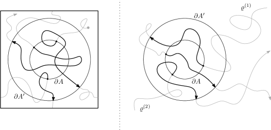
Figure 1: Excursions (pictured as bold pieces of trajectories) for simple random walk on the torus (on the left), and random interlacements (on the right). Note the walk “jumping” from right side of the square to the left one, and from the bottom one to the top one (the torus is pictured as a square). For random interlacements, two trajectories, $\varrho^{1,2}$, intersect the set $A$; the first trajectory produces two excursions, and the second only one.

Now, assume that we want to construct the excursions of $\mathop{\mathrm{RI}}(\alpha)$, say, between $\partial{\mathsf{B}}(y_{0},n)$ and $\partial{\mathsf{B}}(y_{0},cn)$ for some $c>1$ and $y_{0}\in{\mathbb{Z}}^{2}$. Also, (let us identify the torus ${\mathbb{Z}}^{2}_{n_{1}}$ with the square of size $n_{1}$ centered in the origin of ${\mathbb{Z}}^{2}$) we want to construct the excursions of the simple random walk on the torus ${\mathbb{Z}}^{2}_{n_{1}}$ between $\partial{\mathsf{B}}(y_{0},n)$ and $\partial{\mathsf{B}}(y_{0},cn)$, where $n_{1}>n+1$. It turns out that one may build both sets of excursions simultaneously on the same probability space, in such a way that, typically, most of the excursions are present in both sets (obviously, after a translation by $y_{0}$). This is done using the soft local times method; we refer to Section 4 of [16] for the general theory (see also Figure 1 of [16] which gives some quick insight on what is going on), and also to Section 2 of [7]. Here, we describe the soft local times approach in a less formal way. Assume, for definiteness, that we want to construct the simple random walk’s excursions on ${\mathbb{Z}}^{2}_{n_{1}}$, between $\partial A$ and $\partial A^{\prime}$, and suppose that the starting point $x_{0}$ of the walk $X$ does not belong to $A$.

We first describe our approach for the case of the torus. For $x\notin A$ and $y\in\partial A$ let us denote

$$\varphi(x,y)={\mathbb{P}}_{x}[X_{\tau_{1}(A)}=y].$$

For an excursion $Z$ let $\iota(Z)$ be the first point of this excursion, and $\ell(Z)$ be the last one; by definition, $\iota(Z)\in\partial A$ and $\ell(Z)\in\partial A^{\prime}$. Clearly, for the random walk on the torus, the sequence $\big{(}(\iota(Z^{(j)}),\ell(Z^{(j)})),j\geq 1\big{)}$ is a Markov chain with transition probabilities

$$P_{(y,z),(y^{\prime},z^{\prime})}=\varphi(z,y^{\prime}){\mathbb{P}}_{y^{\prime}}[X_{\tau_{1}(\partial A^{\prime})}=z^{\prime}].$$

Now, consider a marked Poisson point process on $\partial A\times{\mathbb{R}}_{+}$ with rate $1$. The (independent) marks are the simple random walk trajectories started from the first coordinate of the Poisson points (i.e., started at the corresponding site of $\partial A$) and run until hitting $\partial A^{\prime}$. Then (see Figure 2; observe that $A$ and $A^{\prime}$ need not be necessarily connected, as shown on the picture)

• let $\xi_{1}$ be the a.s. unique positive number such that there is only one point of the Poisson process on the graph of $\xi_{1}\varphi(x_{0},\cdot)$ and nothing below;

• the mark of the chosen point is the first excursion (call it $Z^{(1)}$) that we obtain;

• then, let $\xi_{2}$ be the a.s. unique positive number such that the graph of $\xi_{1}\varphi(x_{0},\cdot)+\xi_{2}\varphi(\ell(Z^{(1)}),\cdot)$ contains only one point of the Poisson process, and there is nothing between this graph and the previous one;

• the mark $Z^{(2)}$ of this point is our second excursion;

• and so on.

It is possible to show that the sequence of excursions obtained in this way indeed has the same law as the simple random walk’s excursions (in particular, conditional on $\ell(Z^{(k-1)})$, the starting point of $k$th excursion is indeed distributed according to $\varphi(\ell(Z^{(k-1)}),\cdot)$); moreover, the $\xi$’s are i.i.d. random variables with Exponential($1$) distribution.

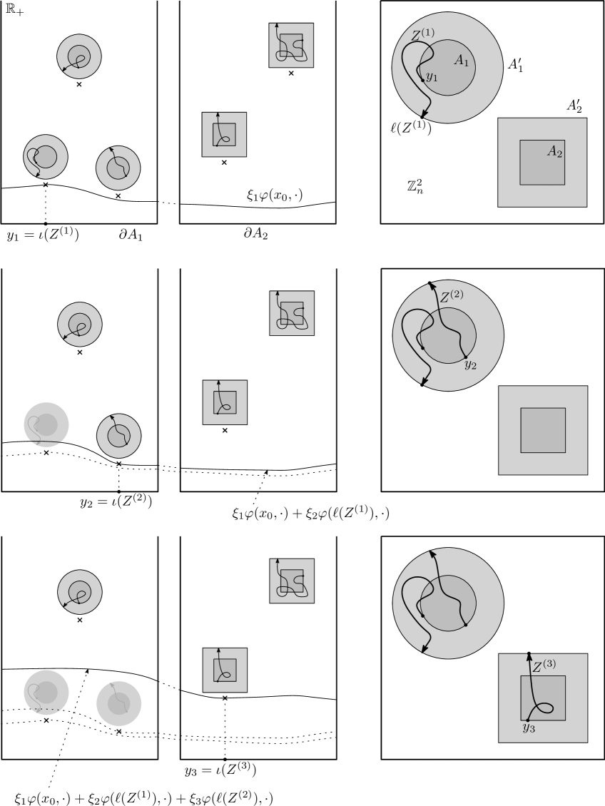
Figure 2: Construction of the first three excursions between $\partial A$ and $\partial A^{\prime}$ on the torus ${\mathbb{Z}}^{2}_{n}$ using the soft local times (here, $A=A_{1}\cup A_{2}$ and $A^{\prime}=A^{\prime}_{1}\cup A^{\prime}_{2}$)

So, let us denote by $\xi_{1},\xi_{2},\xi_{3},\ldots$ a sequence of i.i.d. random variables with Exponential distribution with parameter $1$. According to the above informal description, the soft local time of $k$th excursion is a random vector indexed by $y\in\partial A$, defined as follows:

$$L_{k}(y)=\xi_{1}\varphi(x_{0},y)+\sum_{j=2}^{k}\xi_{j}\varphi(\ell(Z^{(j-1)}),y).$$ (29)

For the random interlacements, the soft local times are defined analogously. Recall that $\mathop{\widehat{\mathrm{hm}}}\nolimits_{A}$ defines the (normalized) harmonic measure on $A$ with respect to the ${\widehat{S}}$-walk. For $x\notin A$ and $y\in\partial A$ let

$${\widehat{\varphi}}(x,y)={\mathbb{P}}_{x}\big{[}{\widehat{S}}_{\widehat{\tau}_{1}(A)}=y,\widehat{\tau}_{1}(A)<\infty\big{]}+{\mathbb{P}}_{x}[\widehat{\tau}_{1}(A)=\infty]\mathop{\widehat{\mathrm{hm}}}\nolimits_{A}(y).$$ (30)

Analogously, for the random interlacements, the sequence $\big{(}(\iota(\widehat{Z}^{(j)}),\ell(\widehat{Z}^{(j)})),j\geq 1\big{)}$ is also a Markov chain, with transition probabilities

$${\widehat{P}}_{(y,z),(y^{\prime},z^{\prime})}={\widehat{\varphi}}(z,y^{\prime}){\mathbb{P}}_{y^{\prime}}\big{[}{\widehat{S}}_{\widehat{\tau}_{1}(\partial A^{\prime})}=z^{\prime}\big{]}.$$

The process of picking the excursions for the random interlacements is quite analogous: if the last excursion was $\widehat{Z}$, we use the probability distribution ${\widehat{\varphi}}(\ell(\widehat{Z}),\cdot)$ to choose the starting point of the next excursion. Clearly, the last term in (30) is needed for ${\widehat{\varphi}}$ to have total mass $1$; informally, if the ${\widehat{S}}$-walk from $x$ does not ever hit $A$, we just take the “next” trajectory of the random interlacements that does hit $A$, and extract the excursion from it (see also (4.10) of [6]). Again, let $\hat{\xi}_{1},\hat{\xi}_{2},\hat{\xi}_{3},\ldots$ be a sequence of i.i.d. random variables with Exponential distribution with parameter $1$. Then, define the soft local time of random interlacement of $k$th excursion as

$$\widehat{L}_{k}(y)=\hat{\xi}_{1}{\widehat{\varphi}}(x_{0},y)+\sum_{j=2}^{k}\hat{\xi}_{j}{\widehat{\varphi}}(\ell(\widehat{Z}^{(j-1)}),y).$$ (31)

Define the following two measures on $\partial A$, one for the random walk on the torus, and the other for random interlacements:

$$\mathop{\mathrm{hm}}\nolimits_{A}^{A^{\prime}}(y) ={\mathbb{P}}_{y}[\tau_{1}(\partial A^{\prime})<\tau_{1}(A)]\Big{(}\sum_{z\in\partial A}{\mathbb{P}}_{z}[\tau_{1}(\partial A^{\prime})<\tau_{1}(A)]\Big{)}^{-1},$$ (32)

$$\mathop{\widehat{\mathrm{hm}}}\nolimits_{A}^{A^{\prime}}(y) ={\mathbb{P}}_{y}[\widehat{\tau}_{1}(\partial A^{\prime})<\widehat{\tau}_{1}(A)]\Big{(}\sum_{z\in\partial A}{\mathbb{P}}_{z}[\widehat{\tau}_{1}(\partial A^{\prime})<\widehat{\tau}_{1}(A)]\Big{)}^{-1}.$$ (33)

Informally, these are “harmonic measures with respect to $A^{\prime}$”; the “real” harmonic measures would be recovered as $A^{\prime}$ expands towards the whole space ${\mathbb{Z}}^{2}$. Similarly to Lemma 6.1 of [6] one can obtain the following important facts: the measure

$$\psi(y,z)=\mathop{\mathrm{hm}}\nolimits_{A}^{A^{\prime}}(y){\mathbb{P}}_{y}[X_{\tau_{1}(\partial A^{\prime})}=z]$$ (34)

is invariant for the Markov chain $(\iota(Z^{(j)}),\ell(Z^{(j)}))$, and the measure

$${\widehat{\psi}}(y,z)=\mathop{\widehat{\mathrm{hm}}}\nolimits_{A}^{A^{\prime}}(y){\mathbb{P}}_{y}\big{[}{\widehat{S}}_{\widehat{\tau}_{1}(\partial A^{\prime})}=z\big{]}$$ (35)

is invariant for the Markov chain $(\iota(\widehat{Z}^{(j)}),\ell(\widehat{Z}^{(j)}))$. Notice also that $\mathop{\mathrm{hm}}\nolimits_{A}^{A^{\prime}}$ and $\mathop{\widehat{\mathrm{hm}}}\nolimits_{A}^{A^{\prime}}$ are the marginals of the stationary measures for the entrance points (i.e., the first coordinate of the Markov chains). In particular, this implies that, almost surely,

$$\lim_{k\to\infty}\frac{L_{k}(y)}{k}=\mathop{\mathrm{hm}}\nolimits_{A}^{A^{\prime}}(y)\quad\text{and}\quad\lim_{k\to\infty}\frac{\widehat{L}_{k}(y)}{k}=\mathop{\widehat{\mathrm{hm}}}\nolimits_{A}^{A^{\prime}}(y),$$

for any $y\in\partial A$.

The next result is needed to have a control on the large and moderate deviation probabilities for soft local times.

Lemma 2.9.

Let $\gamma_{2}>\gamma_{1}>1$ be some fixed constants, assume that $n>3(\gamma_{1}-1)^{-1}$, and abbreviate $n_{1}=\gamma_{2}n$. For the random walk on the torus ${\mathbb{Z}}^{2}_{n_{1}}$, abbreviate $A={\mathsf{B}}(n)$ and $A^{\prime}={\mathsf{B}}(\gamma_{1}n)$. For the random interlacements, abbreviate $B={\mathsf{B}}(y_{0},n)$ and $B^{\prime}={\mathsf{B}}(y_{0},\gamma_{1}n)$, where $y_{0}\in{\mathbb{Z}}^{2}$ is such that $\|y_{0}\|\geq 2\gamma_{1}n$. Then there exist positive constants $c,c_{1},c_{2}$ such that for all $k\geq 2$ and all $\theta\in(0,(\ln k)^{-1})$ we have

$${\mathbb{P}}\Big{[}\sup_{y\in\partial A}\big{|}L_{k}(y)-k\mathop{\mathrm{hm}}\nolimits_{A}^{A^{\prime}}(y)\big{|}\geq\frac{c\sqrt{k}+\theta k}{n_{1}}\Big{]}\leq c_{1}e^{-c_{2}\theta^{2}k},$$ (36)

$${\mathbb{P}}\Big{[}\sup_{y\in\partial B}\big{|}\widehat{L}_{k}(y)-k\mathop{\widehat{\mathrm{hm}}}\nolimits_{B}^{B^{\prime}}(y)\big{|}\geq\frac{c\sqrt{k}+\theta k}{n}\Big{]}\leq c_{1}e^{-c_{2}\theta^{2}k}.$$ (37)

Proof.

We prove only (36), the proof of (37) is completely analogous. Due to Lemma 2.4, it is enough to show that for some (sufficiently large) $c^{\prime},c^{\prime}_{1}$ and (sufficiently small) $c^{\prime}_{2}>0$

$${\mathbb{P}}\Big{[}\sup_{y\in\partial A}\Big{|}\frac{L_{k}(y)}{\mathop{\mathrm{hm}}\nolimits_{A}(y)}-k\frac{\mathop{\mathrm{hm}}\nolimits_{A}^{A^{\prime}}(y)}{\mathop{\mathrm{hm}}\nolimits_{A}(y)}\Big{|}\geq c^{\prime}\sqrt{k}+\theta k\Big{]}\leq c^{\prime}_{1}e^{-c^{\prime}_{2}\theta^{2}k}.$$ (38)

We prove the above inequality in the following way:

1. Using renewals, we split the sequence of excursions into independent blocks.

2. We show that controlling that sequence of i.i.d. blocks of excursions is enough to be able to control the original sequence.

3. Then, we obtain an upper bound on the expectation of the sum of independent blocks. For this, we estimate the bracketing entropy integral and then use an inequality due to Pollard.

4. Finally, we control the deviation (from the expectation) probabilities, using a suitable concentration inequality.

Step 1. Again, Lemma 2.4 implies that there exists $\lambda>0$ such that for all $x\in\partial A^{\prime}$ and $y\in\partial A$ we have $\varphi(x,y)\geq 2\lambda\mathop{\mathrm{hm}}\nolimits_{A_{1}}^{A^{\prime}_{1}}(y)$. Consider a sequence of random variables $\eta_{1},\eta_{2},\eta_{3},\ldots$, independent of everything, and such that ${\mathbb{P}}[\eta_{j}=1]=1-{\mathbb{P}}[\eta_{j}=0]=\lambda$ for all $j$. For $j\geq 1$ define $\rho_{j}=m$ iff $\eta_{1}+\cdots+\eta_{m}=j$ and $\eta_{m}=1$ (that is, $\rho_{j}$ is the position of $j$th “$1$” in the $\eta$-sequence). The idea is that we force the Markov chain to have renewals at times when $\eta_{\cdot}=1$, and then try to approximate the soft local time by a sum of independent random variables. More precisely, assume that $\ell(Z^{(j-1)})=x$. Then, we choose the starting point $\iota(Z^{(j)})$ of the $j$th excursion in the following way

$$\iota(Z^{(j)})\sim\begin{cases}\displaystyle\frac{1}{1-\lambda}\big{(}\varphi(x,\cdot)-\lambda\mathop{\mathrm{hm}}\nolimits_{A_{1}}^{A^{\prime}_{1}}\big{)},&\text{if }\eta_{j}=0,\\ \mathop{\mathrm{hm}}\nolimits_{A_{1}}^{A^{\prime}_{1}},\phantom{\int\limits^{A^{B}}}&\text{if }\eta_{j}=1.\end{cases}$$

Denote $W_{0}(\cdot)=L_{\rho_{1}-1}(\cdot)$, and

$$W_{j}(\cdot)=L_{\rho_{j+1}-1}(\cdot)-L_{\rho_{j}-1}(\cdot)$$

for $j\geq 1$. By construction, it holds that $(W_{j},j\geq 1)$ is a sequence of i.i.d. random vectors. Also, it is straightforward to obtain that ${\mathbb{E}}W_{j}(y)=\lambda^{-1}\mathop{\mathrm{hm}}\nolimits_{A_{1}}^{A^{\prime}_{1}}(y)$ for all $y\in\partial A$ and all $j\geq 1$.

Step 2. Now, we are going to show that, to prove (38), it is enough to prove that, for some positive constants $c^{\prime\prime},c^{\prime\prime}_{1},c^{\prime\prime}_{2}$

$${\mathbb{P}}\Big{[}\sup_{y\in\partial A}\Big{|}\frac{\sum_{j=1}^{m}W_{j}(y)}{\mathop{\mathrm{hm}}\nolimits_{A}(y)}-\lambda^{-1}m\frac{\mathop{\mathrm{hm}}\nolimits_{A}^{A^{\prime}}(y)}{\mathop{\mathrm{hm}}\nolimits_{A}(y)}\Big{|}\geq c^{\prime\prime}\sqrt{m}+\theta m\Big{]}\leq c^{\prime\prime}_{1}e^{-c^{\prime\prime}_{2}\theta^{2}m}.$$ (39)

for all $m\geq 2$ and all $\theta\in(0,(\ln m)^{-1})$. Observe that we can assume without loss of generality that $c^{\prime\prime}_{1}\leq\frac{1}{2}$; indeed, if the above holds with some $c^{\prime\prime}_{1}>0$, then, by increasing $c^{\prime\prime}$ (and, possibly, decreasing $c^{\prime\prime}_{2}$; note that $(c^{\prime\prime}+h)\sqrt{m}+\theta m=c^{\prime\prime}\sqrt{m}+(\theta+\frac{h}{\sqrt{m}})m$) we can put an arbitrarily small constant before the exponent in the right-hand side.

Abbreviate

$$R_{k} =\sup_{y\in\partial A}\Big{|}\frac{L_{k}(y)}{\mathop{\mathrm{hm}}\nolimits_{A}(y)}-k\frac{\mathop{\mathrm{hm}}\nolimits_{A}^{A^{\prime}}(y)}{\mathop{\mathrm{hm}}\nolimits_{A}(y)}\Big{|},$$

and

$${\widetilde{R}}_{k} =\sup_{y\in\partial A}\Big{|}\frac{\sum_{j=1}^{k}W_{j}(y)}{\mathop{\mathrm{hm}}\nolimits_{A}(y)}-\lambda^{-1}k\frac{\mathop{\mathrm{hm}}\nolimits_{A}^{A^{\prime}}(y)}{\mathop{\mathrm{hm}}\nolimits_{A}(y)}\Big{|}.$$

Let us first show that (39) implies

$${\mathbb{P}}\Big{[}\max_{i\in[m,2m]}{\widetilde{R}}_{i}\geq 4c^{\prime\prime}\sqrt{m}+5\theta m\Big{]}\leq 2c^{\prime\prime}_{1}e^{-3c^{\prime\prime}_{2}\theta^{2}m}.$$ (40)

For this, define the random variable

$$N=\min\big{\{}i\in[m,2m]:{\widetilde{R}}_{i}\geq 4c^{\prime\prime}\sqrt{m}+5\theta m\big{\}}$$

(by definition, $\min\emptyset:=+\infty$), so the left-hand side of (40) is equal to ${\mathbb{P}}\big{[}N\in[m,2m]\big{]}$. Note also that the right-hand side of (39) does not exceed $\frac{1}{2}$ (recall that we assumed that $c^{\prime\prime}_{1}\leq\frac{1}{2}$). Now, (39) implies (note that $\sqrt{3}<4-\sqrt{2}$)

$$c^{\prime\prime}_{1}e^{-3c^{\prime\prime}_{2}\theta^{2}m} \geq{\mathbb{P}}\big{[}{\widetilde{R}}_{3m}\geq c^{\prime\prime}\sqrt{3m}+3\theta m\big{]}$$

$$\geq\sum_{j=m}^{2m}{\mathbb{P}}[N=j]{\mathbb{P}}\big{[}{\widetilde{R}}_{3m-j}<c^{\prime\prime}\sqrt{2m}+2\theta m\big{]}$$

$$\geq{\mathbb{P}}\big{[}N\in[m,2m]\big{]}\times\min_{j\in[m,2m]}{\mathbb{P}}\big{[}{\widetilde{R}}_{3m-j}<c^{\prime\prime}\sqrt{3m-j}+\theta(3m-j)\big{]}$$

$$\geq\frac{1}{2}{\mathbb{P}}\big{[}N\in[m,2m]\big{]}$$

for all large enough $m$.

Next, let us denote $\sigma_{k}=\min\{j\geq 1:\rho_{j}>k\}$. By (32) and Lemma 2.5 we may assume that $\frac{1}{2}\leq\frac{\mathop{\mathrm{hm}}\nolimits_{A}^{A^{\prime}}(y)}{\mathop{\mathrm{hm}}\nolimits_{A}(y)}\leq 2$, and, due to Lemma 2.4, $\frac{L_{k}(y)}{\mathop{\mathrm{hm}}\nolimits_{A}(y)}\leq\tilde{c}$ for some $\tilde{c}>0$. So, we can write

$$R_{k}\leq{\widetilde{R}}_{\sigma_{k}}+2|\lambda^{-1}\sigma_{k}-k|+\tilde{c}\sum_{i=k+1}^{\rho_{\sigma_{k}}}\xi_{i}.$$ (41)

Now, observe that $\sigma_{k}-1$ is a Binomial$(k,\lambda)$ random variable, and $\rho_{\sigma_{k}}-k$ is Geometric$(\lambda)$. Therefore, the last two terms in the right-hand side of (41) are easily dealt with; that is, we may write for large enough $\hat{c}>0$

$${\mathbb{P}}\big{[}2|\lambda^{-1}\sigma_{k}-k|\geq\hat{c}\sqrt{k}+\theta k\big{]} \leq c_{4}e^{-c^{\prime}_{4}\theta^{2}k},$$ (42)

$${\mathbb{P}}\Big{[}\tilde{c}\sum_{i=k+1}^{\rho_{\sigma_{k}}}\xi_{i}\geq\theta k\Big{]} \leq e^{-c_{5}\lambda\theta k}.$$ (43)

Then, using (40) together with (42)–(43), we obtain (recall (38))

$${\mathbb{P}}\Big{[}R_{k}\geq\big{(}4c^{\prime\prime}(\textstyle\frac{2\lambda}{3})^{1/2}+\hat{c}\big{)}\sqrt{k}+\big{(}\textstyle\frac{10}{3}\lambda+2\big{)}\theta k\Big{]}$$

$$\leq{\mathbb{P}}\Big{[}\max_{i\in[\frac{2}{3}\lambda k,\frac{4}{3}\lambda k]}{\widetilde{R}}_{i}\geq 4c^{\prime\prime}(\textstyle\frac{2\lambda}{3})^{1/2}\sqrt{k}+5\theta\cdot\textstyle\frac{2}{3}\lambda k\Big{]}+{\mathbb{P}}\big{[}\sigma_{k}\notin[\frac{2}{3}\lambda k,\frac{4}{3}\lambda k]\big{]}$$

$$\quad+{\mathbb{P}}\big{[}2|\lambda^{-1}\sigma_{k}-k|\geq\hat{c}\sqrt{k}+\theta k\big{]}+{\mathbb{P}}\Big{[}\tilde{c}\sum_{i=k+1}^{\rho_{\sigma_{k}}}\xi_{i}\geq\theta k\Big{]}$$

$$\leq 2c^{\prime\prime}_{1}e^{-2\lambda c^{\prime\prime}_{2}\theta^{2}k}+e^{-c_{6}\lambda k}+c_{4}e^{-c^{\prime}_{4}\theta^{2}k}+e^{-c_{5}\lambda\theta k},$$

and this shows that it is indeed enough for us to prove (39).

Step 3. Now, the advantage of (39) is that we are dealing with i.i.d. random vectors there, so it is convenient to use some machinery from the theory of empirical processes. First, the idea is to use the Pollard inequality (cf. (1.2) of [21]) to prove that

$${\mathbb{E}}{\widetilde{R}}_{k}\leq c_{7}\sqrt{k}$$ (44)

for some $c_{7}>0$ (note that the above estimate is uniform with respect to the size of $\partial A$). To use the language of empirical processes, we are dealing here with random elements of the form ${\widetilde{W}}_{j}=\frac{W_{j}}{\mathop{\mathrm{hm}}\nolimits_{A}}$ which are positive vectors indexed by sites of $\partial A$. Let also $Y$ be a generic positive vector indexed by sites of $\partial A$. For $y\in\partial A$ let ${\mathcal{E}}_{y}$ be the evaluation functional at $y$: ${\mathcal{E}}_{y}(Y):=Y(y)$. Denote by ${\mathcal{F}}=\{{\mathcal{E}}_{y},y\in\partial A\}$ the class of functions we are interested in; then, we need to find an upper bound on the expectation of $\sup_{f\in{\mathcal{F}}}|\sum_{j=1}^{k}f({\widetilde{W}}_{j})-{\mathbb{E}}f({\widetilde{W}}_{j})|$. Using the terminology of [21], let $\|f\|_{2}:=\sqrt{{\mathbb{E}}f^{2}({\widetilde{W}})}$, where ${\widetilde{W}}$ has the same law as the ${\widetilde{W}}_{j}$’s above. Consider the envelope function $F$ defined by

$$F(Y)=\sup_{y\in\partial A}{\mathcal{E}}_{y}(Y)=\sup_{y\in\partial A}Y(y).$$

Due to Lemma 2.4, we have

$$\|F\|_{2}\leq c_{8}.$$ (45)

Let us define the bracketing entropy integral

$$J_{[\,]}\big{(}1,{\mathcal{F}},\|\cdot\|_{2}\big{)}=\int_{0}^{1}\sqrt{1+\ln N_{[\,]}(s\|F\|_{2},{\mathcal{F}},\|\cdot\|_{2})}ds.$$ (46)

In the above expression, $N_{[\,]}(\delta,{\mathcal{F}},\|\cdot\|_{2})$ is the so-called bracketing number: the minimal number of brackets $[f,g]=\{h:f\leq h\leq g\}$ needed to cover ${\mathcal{F}}$ of size $\|g-f\|_{2}$ smaller than $\delta$. We now recall (1.2) of [21]:

$${\mathbb{E}}{\widetilde{R}}_{k}\leq cJ_{[\,]}(1,{\mathcal{F}},\|\cdot\|_{2})\|F\|_{2}\sqrt{k};$$ (47)

so, to prove (44), we need to obtain an upper bound on the bracketing entropy integral.

Let us define “arc intervals” on $\partial A$ by $I(y,r)=\{z\in\partial A:\|y-z\|\leq r\}$, where $y\in\partial A,r>0$. Observe that $I(y,r)=\{y\}$ in case $r<1$. Define

$$f^{y,r}(Y)=\inf_{z\in I(y,r)}Y(z),\quad g^{y,r}(Y)=\sup_{z\in I(y,r)}Y(z);$$

in order to cover ${\mathcal{F}}$, we are going to use brackets of the form $[f^{y,r},g^{y,r}]$. Notice that if $z\in I(y,r)$ then ${\mathcal{E}}_{z}\in[f^{y,r},g^{y,r}]$, so a covering of ${\mathcal{F}}$ by the above brackets corresponds to a covering of $\partial A$ by “intervals” $I(\cdot,\cdot)$. Let us estimate the size of the bracket $[f^{y,r},g^{y,r}]$; it is here that Proposition 1.3 comes into play. We have

$$\|g^{y,r}-f^{y,r}\|_{2} =\textstyle\sqrt{{\mathbb{E}}\big{|}\!\sup_{z\in I(y,r)}{\widetilde{W}}(z)-\inf_{z\in I(y,r)}{\widetilde{W}}(z)\big{|}}$$

$$\leq c_{9}r^{\beta}\|\xi_{1}+\cdots+\xi_{\rho}\|_{2}$$

$$\leq 2c_{9}\lambda^{-1}r^{\beta};$$ (48)

in the above calculation, $\rho$ is a Geometric random variable with success probability $\lambda$, $\xi$’s are i.i.d. Exponential(1) random variables also independent of $\rho$, and we use an elementary fact that $\xi_{1}+\cdots+\xi_{\rho}$ is then also Exponential with mean $\lambda^{-1}$.

Then, recall (45), and observe that, for any $\delta>0$ it is possible to cover ${\mathcal{F}}$ with $|\partial A|=O(n_{1})$ brackets of size smaller than $\delta$ (just cover each site separately with brackets $[f^{\cdot,1/2},g^{\cdot,1/2}]$ of zero size). That is, for any $s>0$ it holds that

$$N_{[\,]}\big{(}s\|F\|_{2},{\mathcal{F}},\|\cdot\|_{2}\big{)}\leq c_{10}n_{1}.$$ (49)

Next, if $s\geq c_{11}n_{1}^{-\beta}$, then we are able to use intervals of size $r=O(n_{1}s^{1/\beta})$ to cover $\partial A$, so we have

$$N_{[\,]}\big{(}s\|F\|_{2},{\mathcal{F}},\|\cdot\|_{2}\big{)}=O(n_{1}/r)\leq c_{12}s^{-1/\beta}.$$ (50)

So (recall (46)) the bracketing entropy integral can be bounded above by

$$c_{11}n_{1}^{-\beta}\sqrt{1+\ln(c_{10}n_{1})}+\int_{c_{11}n_{1}^{-\beta}}^{1}\sqrt{1+\ln(c_{12}s^{-1/\beta})}\,ds\leq c_{13}.$$

Then, using (47), we obtain (44).

Step 4. Here, let us use Theorem 4 of [1] to prove that (with $t=\theta k$)

$${\mathbb{P}}\big{[}{\widetilde{R}}_{k}\geq 2{\mathbb{E}}{\widetilde{R}}_{k}+t\big{]}\leq c_{14}e^{-c_{15}t^{2}/k}+c_{16}e^{-c_{17}t/\ln k};$$ (51)

this is enough for us since, due to the assumption $\theta<(\ln k)^{-1}$ it holds that

$$c_{14}e^{-c_{15}t^{2}/k}+c_{16}e^{-c_{17}t/\ln k}\leq c_{18}e^{-c_{19}\theta^{2}k}.$$

To apply that theorem, we only need to estimate the $\psi_{1}$-Orlicz norm of ${\mathcal{E}}_{y}({\widetilde{W}})$, see Definition 1 of [1]. But (recall the notations just below (48)) it holds that ${\mathcal{E}}_{y}({\widetilde{W}})$ is stochastically bounded above by $const\times$Exponential($\lambda$) random variable, so the $\psi_{1}$-Orlicz norm is uniformly bounded above. The factor $\ln k$ in the last term in the right-hand side of (51) comes from the Pisier’s inequality, cf. (13) of [1].

Finally, combining (44) and (51), we obtain (39), and, as observed before, this is enough to conclude the proof of Lemma 2.9. ∎

Next, we need a fact that one may call the consistency of soft local times. Assume that we need to construct excursions of some process (i.e., random walk, random interlacements, or just independent excursions) between $\partial A$ and $\partial A^{\prime}$; let $(\widehat{L}_{k}(y),y\in\partial A)$ be the soft local time of $k$th excursion (of random interlacements, for definiteness). On the other hand, we may be interested in simultaneously constructing the excursions also between $\partial A_{1}$ and $\partial A^{\prime}_{1}$, where $A^{\prime}\cap A^{\prime}_{1}=\emptyset$ and $A_{1}\subset A^{\prime}_{1}$. Let $(\widehat{L}^{*}_{k}(y),y\in\partial A)$ be the soft local time at the moment when $k$th excursion between $\partial A$ and $\partial A^{\prime}$ was chosen in this latter construction. We need the following simple fact:

Lemma 2.10.

It holds that

$$\big{(}\widehat{L}_{k}(y),y\in\partial A\big{)}\stackrel{{\scriptstyle\text{\tiny law}}}{{=}}\big{(}\widehat{L}^{*}_{k}(y),y\in\partial A\big{)}$$

for all $k\geq 1$.

Proof.

First, due to the memoryless property of the Poisson process, it is clearly enough to prove that $\widehat{L}_{1}\stackrel{{\scriptstyle\text{\tiny law}}}{{=}}\widehat{L}^{*}_{1}$. This, by its turn, can be easily obtained from the fact that $\widehat{Z}^{(1)}\stackrel{{\scriptstyle\text{\tiny law}}}{{=}}\widehat{Z}^{(1),*}$, where $\widehat{Z}^{(1)}$ and $\widehat{Z}^{(1),*}$ are the first excursions between $\partial A$ and $\partial A^{\prime}$ chosen in both constructions. ∎

Also, we need to be able to control the number of excursions $N^{*}_{t}$ up to time $t$ on the torus ${\mathbb{Z}}^{2}_{n}$ between $\partial{\mathsf{B}}(\gamma_{1}n)$ and $\partial{\mathsf{B}}(\gamma_{2}n)$, $\gamma_{1}<\gamma_{2}<1/2$.

Lemma 2.11.

For all large enough $n$, all $t\geq n^{2}$ and all $\delta>0$ we have

$${\mathbb{P}}\Big{[}(1-\delta)\frac{\pi t}{2n^{2}\ln(\gamma_{2}/\gamma_{1})}\leq N^{*}_{t}\leq(1+\delta)\frac{\pi t}{2n^{2}\ln(\gamma_{2}/\gamma_{1})}\Big{]}\geq 1-c_{1}\exp\Big{(}-\frac{c_{2}\delta^{2}t}{n^{2}}\Big{)},$$ (52)

where $c_{1,2}$ are positive constants depending on $\gamma_{1,2}$.

Proof.

Note that there is a much more general result on the large deviations of the excursion counts for the Brownian motion (the radii of the concentric disks need not be of order $n$), see Proposition 8.10 of [3]. So, we give the proof of Lemma 2.11 in a rather sketchy way. First, let us rather work with the two-sided stationary version of the walk $X=(X_{j},j\in{\mathbb{Z}})$ (so that $X_{j}$ is uniformly distributed on ${\mathbb{Z}}^{2}_{n}$ for any $j\in{\mathbb{Z}}$). For $x\in\partial{\mathsf{B}}(\gamma_{1}n)$ define the set

$$J_{x} =\big{\{}k\in{\mathbb{Z}}:X_{k}=x,\text{ there exists }i<k\text{ such that }X_{i}\in\partial{\mathsf{B}}(\gamma_{2}n)$$

$$\qquad\qquad\qquad\qquad\qquad\text{ and }X_{m}\in{\mathsf{B}}(\gamma_{2}n)\setminus({\mathsf{B}}(\gamma_{1}n)\cup\partial{\mathsf{B}}(\gamma_{2}n))\text{ for }i<m<k\big{\}},$$

and let $J=\bigcup_{x\in\partial{\mathsf{B}}(\gamma_{1}n)}J_{x}$. Now, Lemma 2.5 together with the reversibility argument used in Lemma 6.1 of [6] imply that

$${\mathbb{P}}[0\in J_{x}]={\mathbb{P}}[X_{0}=x]{\mathbb{P}}_{x}\big{[}\tau_{1}(\partial{\mathsf{B}}(\gamma_{2}n))<\tau_{1}({\mathsf{B}}(\gamma_{1}n))\big{]}=n^{-2}\frac{\mathop{\mathrm{hm}}\nolimits_{{\mathsf{B}}(\gamma_{1}n)}(x)}{\frac{2}{\pi}\ln\frac{\gamma_{2}}{\gamma_{1}}+O(n^{-1})},$$

so (since $\mathop{\mathrm{hm}}\nolimits_{{\mathsf{B}}(\gamma_{1}n)}(\cdot)$ sums to $1$)

$${\mathbb{P}}[0\in J]=\Big{(}\frac{2n^{2}}{\pi}\ln\frac{\gamma_{2}}{\gamma_{1}}+O(n)\Big{)}^{-1}.$$ (53)

Let us write $J=\{\sigma_{j},j\in{\mathbb{Z}}\}$, where $\sigma_{-1}<0$, $\sigma_{0}\geq 0$, and $\sigma_{j}<\sigma_{j+1}$ for all $j\in{\mathbb{Z}}$. As noted just after (32)–(33), the invariant entrance measure to ${\mathsf{B}}(\gamma_{1}n)$ for excursions is $\nu=\mathop{\mathrm{hm}}\nolimits_{{\mathsf{B}}(\gamma_{1}n)}^{{\mathsf{B}}(\gamma_{2}n)}$. Let ${\mathbb{E}}_{\nu}^{*}$ be the expectation for the walk with $X_{0}\sim\nu$ and conditioned on $0\in J$ (that is, for the cycle-stationary version of the walk). Then, in a standard way one obtains from (53) that

$${\mathbb{E}}_{\nu}^{*}\sigma_{1}={\mathbb{E}}_{\nu}^{*}(\sigma_{1}-\sigma_{0})=\frac{2n^{2}}{\pi}\ln\frac{\gamma_{2}}{\gamma_{1}}+O(n).$$ (54)

Note also that in this setup (radii of disks of order $n$) it is easy to control the tails of $\sigma_{1}-\sigma_{0}$ since in each interval of length $O(n^{2})$ there is at least one complete excursion with uniformly positive probability (so there is no need to apply the Khasminskii’s lemma, as one usually does for proving results on large deviations of excursion counts). To conclude the proof of Lemma 2.11, it is enough to apply a renewal argument similar to the one used in the proof of Lemma 2.9 (and in Section 8 of [3]). ∎

3 Proofs of the main results

Proof of Proposition 1.3.

Fix some $x,y,z$ as in the statement of the proposition. We need the following fact:

Lemma 3.1.

We have

$$H_{A_{n}}(x,u)={\mathbb{E}}_{u}\sum_{j=1}^{\tau_{1}(\partial A_{n})}{\mathbf{1}}{\{S_{j}=x\}}=\frac{1}{2d}\sum_{\begin{subarray}{c}v\sim u:\\ v\in A_{n}\setminus\partial A_{n}\end{subarray}}G_{A_{n}}(v,x)$$ (55)

(that is, $H_{A_{n}}(x,u)$ equals the mean number of visits to $x$ before hitting $\partial A_{n}$, starting from $u$) for all $u\in\partial{\mathsf{B}}(n)$.

Proof.

This follows from a standard reversibility argument. Indeed, write (the sums below are over all nearest-neighbor trajectories beginning in $x$ and ending in $u$ that do not touch $\partial A_{n}$ before entering $u$; $\varrho^{*}$ stands for $\varrho$ reversed, $|\varrho|$ is the number of edges in $\varrho$, and $k(\varrho)$ is the number of times $\varrho$ was in $x$)

$$H_{A_{n}}(x,u) =\sum_{\varrho}(2d)^{-|\varrho|}$$

$$=\sum_{\varrho}(2d)^{-|\varrho^{*}|}$$

$$=\sum_{j=1}^{\infty}\sum_{\varrho:k(\varrho)=j}(2d)^{-|\varrho^{*}|},$$

and observe that the $j$th term in the last line is equal to the probability that $x$ is visited at least $j$ times (starting from $u$) before hitting $\partial A_{n}$. This implies (55). ∎

Note that, by Lemma 2.4 we have also

$$\frac{c_{1}}{n^{d-1}}\leq H_{A_{n}}(x,u)\leq\frac{c_{2}}{n^{d-1}},$$ (56)

and, as a consequence (since $$\mathop{\mathrm{hm}}\nolimits_{{\mathsf{B}}(n)}(u) x^{\prime}\in\partial{\mathsf{B}}((1+2\varepsilon)n) H_{A_{n}}(x^{\prime},u)$$ is a convex combination in  of )

$$\frac{c_{1}}{n^{d-1}}\leq\mathop{\mathrm{hm}}\nolimits_{{\mathsf{B}}(n)}(u)\leq\frac{c_{2}}{n^{d-1}}$$ (57)

for all $u\in\partial{\mathsf{B}}(n)$. Therefore, without restricting generality we may assume that $\|y-z\|\leq(\varepsilon/9)n$, since if $\|y-z\|$ is of order $n$, then (14) holds for large enough $C$.

So, using Lemma 3.1, we can estimate the difference between the mean numbers of visits to one fixed site in the interior of the annulus starting from two close sites at the boundary, instead of dealing with hitting probabilities of two close sites starting from that fixed site.

Then, to obtain (14), we proceed in the following way.

• Observe that, to go from a site $u\in\partial{\mathsf{B}}(n)$ to $x$, the particle needs to go first to $\partial{\mathsf{B}}((1+\varepsilon)n)$; we then prove that the probability of that is “almost” proportional to $\mathop{\mathrm{hm}}\nolimits_{{\mathsf{B}}(n)}(u)$, see (58).

• In (60) we introduce two walks conditioned on hitting $\partial{\mathsf{B}}((1+\varepsilon)n)$ before returning to $\partial{\mathsf{B}}(n)$, starting from $y,z\in\partial{\mathsf{B}}(n)$. The idea is that they will likely couple before reaching $\partial{\mathsf{B}}((1+\varepsilon)n)$.

• More precisely, we prove that each time the distance between the original point on $\partial{\mathsf{B}}(n)$ and the current position of the (conditioned) walk is doubled, there is a uniformly positive chance that the coupling of the two walks succeeds (see the argument just after (67)).

• To prove the above claim, we define two sequences $(U_{k})$ and $(V_{k})$ of subsets of the annulus ${\mathsf{B}}((1+\varepsilon)n)\setminus{\mathsf{B}}(n)$, as shown on Figure 3. Then, we prove that the positions of the two walks on first hitting of $V_{k}$ can be coupled with uniformly positive probability, regardless of their positions on first hitting of $V_{k-1}$. For that, we need two technical steps:

  • If one of the two conditioned walks hits $V_{k-1}$ at a site which is “too close” to $\partial{\mathsf{B}}(n)$ (look at the point $Z_{k-1}$ on Figure 3), we need to assure that the walker can go “well inside” the set $U_{k}$ with at least constant probability (see (63)).

  • If the (conditioned) walk is already “well inside” the set $U_{k}$, then one can apply the Harnack inequality to prove that the exit probabilities are comparable in the sense of (67).

• There are $O\big{(}\ln\frac{n}{\|y-z\|}\big{)}$ “steps” on the way to $\partial{\mathsf{B}}((1+\varepsilon)n)$, and the coupling is successful on each step with uniformly positive probability. So, in the end the coupling fails with probability polynomially small in $\frac{n}{\|y-z\|}$, cf. (68).

• Then, it only remains to gather the pieces together (the argument after (69)). The last technical issue is to show that, even if the coupling does not succeed, the difference of expected hit counts cannot be too large; this follows from (15) and Lemma 2.3.

We now pass to the detailed arguments. By Lemma 2.5 we have for any $u\in\partial{\mathsf{B}}(n)$

$${\mathbb{P}}_{u}\big{[}\tau_{0}(\partial{\mathsf{B}}((1+\varepsilon)n))<\tau_{1}(\partial{\mathsf{B}}(n))\big{]}=\begin{cases}\displaystyle\frac{\mathop{\mathrm{hm}}\nolimits_{{\mathsf{B}}(n)}(u)}{\frac{2}{\pi}\ln(1+\varepsilon)+O(n^{-1})},&\text{for }d=2,\\ \displaystyle\frac{\mathop{\mathrm{cap}}({\mathsf{B}}(n))\mathop{\mathrm{hm}}\nolimits_{{\mathsf{B}}(n)}(u)}{1-(1+\varepsilon)^{-(d-2)}+O(n^{-1})}\vphantom{\int\limits^{A^{B}}},&\text{for }d\geq 3,\end{cases}$$ (58)

so, one can already notice that the probabilities to escape to $\partial{\mathsf{B}}((1+\varepsilon)n)$ normalized by the harmonic measures are roughly the same for all sites of $\partial{\mathsf{B}}(n)$. Define the events

$$F_{j}=\big{\{}\tau_{0}(\partial{\mathsf{B}}((1+\varepsilon)n))<\tau_{j}(\partial{\mathsf{B}}(n))\big{\}}$$ (59)

for $j=0,1$. For $v\in{\mathsf{B}}((1+\varepsilon)n)\setminus{\mathsf{B}}(n)$ denote $h(v)={\mathbb{P}}_{v}[F]$; clearly, $h$ is a harmonic function inside the annulus ${\mathsf{B}}((1+\varepsilon)n)\setminus{\mathsf{B}}(n)$, and the simple random walk on the annulus conditioned on $F_{0}$ is in fact a Markov chain (that is, the Doob’s $h$-transform of the simple random walk) with transition probabilities

$$\widetilde{P}_{v,w}=\begin{cases}\displaystyle\frac{h(w)}{2dh(v)},&v\in{\mathsf{B}}((1+\varepsilon)n)\setminus({\mathsf{B}}(n)\cup\partial{\mathsf{B}}((1+\varepsilon)n)),w\sim v,\\ 0,&\text{otherwise}.\end{cases}$$ (60)

On the first step (starting at $u\in\partial{\mathsf{B}}(n)$), the transition probabilities of the conditioned walk are described in the following way: the walk goes to $v\notin{\mathsf{B}}(n)$ with probability

$$h(v)\Bigg{(}\sum_{\begin{subarray}{c}v^{\prime}\notin{\mathsf{B}}(n):\\ v^{\prime}\sim u\end{subarray}}h(v^{\prime})\Bigg{)}^{-1}.$$

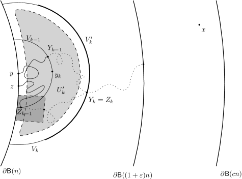
Figure 3: On the coupling of conditioned walks in the proof of Proposition 1.3. Here, $Y_{k-1}$ and $Z_{k-1}$ are positions of the walks started in $y$ and $z$, and we want to couple their exit points on $V^{\prime}_{k}$. The $y$-walk is already in $U^{\prime}_{k}$, but we need to force the $z$-walk to advance to $U^{\prime}_{k}$ in the set $\Psi(Z_{k-1},\|y-z\|2^{k-1})$ (dark grey on the picture), so that the Harnack inequality would be applicable.

Let $k_{0}=\max\{j:3\|y-z\|2^{j}<\varepsilon n\}$, and let us define the sets

$$U_{k} ={\mathsf{B}}(y,3\|y-z\|2^{k})\setminus\big{(}{\mathsf{B}}(n)\setminus\partial{\mathsf{B}}(n)\big{)},$$

$$V_{k} =\partial U_{k}\setminus\partial{\mathsf{B}}(n),$$

for $k=1,\ldots,k_{0}$, see Figure 3. Also, define $y_{k}$ to be the closest integer point to $y+3\|y-z\|2^{k}\frac{y}{\|y\|}$. Clearly, it holds that

$$k_{0}\geq c_{2}\ln\frac{c_{3}\varepsilon n}{\|y-z\|}.$$ (61)

Denote by ${\widetilde{S}}^{(1)}$ and ${\widetilde{S}}^{(2)}$ the conditioned random walks started from $y$ and $z$. For $k=1,\ldots,k_{0}$ denote $Y_{k}={\widetilde{S}}^{(1)}_{{\tilde{\tau}}_{1}(V_{k})}$, $Z_{k}={\widetilde{S}}^{(2)}_{{\tilde{\tau}}_{1}(V_{k})}$, where ${\tilde{\tau}}_{1}$ is the hitting time for the ${\widetilde{S}}$-walks, defined as in (2). The goal is to couple $(Y_{1},\ldots,Y_{k_{0}})$ and $(Z_{1},\ldots,Z_{k_{0}})$ in such a way that with high probability there exists $k_{1}\leq k_{0}$ such that $Y_{j}=Z_{j}$ for all $j=k_{1},\ldots,k_{0}$; we denote by $\Upsilon$ the corresponding coupling event. Clearly, this generates a shift-coupling of ${\widetilde{S}}^{(1)}$ and ${\widetilde{S}}^{(2)}$; if we managed to shift-couple them before they reach $\partial{\mathsf{B}}((1+\varepsilon)n)$, then the number of visits to $x$ will be the same.

For $v\in{\mathbb{R}}^{d}$ let $\ell_{v}=\{rv,r>0\}$ be the ray in $v$’s direction. Now, for any $v$ with $n<\|v\|\leq(1+\varepsilon)n$ and $s\in(0,\varepsilon n)$ define the (discrete) set

$$\Psi(v,s)=\big{\{}u\in{\mathbb{Z}}^{d}:n<\|u\|\leq n+s,\mathop{\mathrm{dist}}(u,\ell_{v})\leq s/2\big{\}}.$$

Denote also by

$$\partial^{+}\Psi(v,s)=\big{\{}u\in\partial\Psi(v,s):n+s-1<\|u\|\leq n+s\big{\}}$$

the “external part” of the boundary of $\Psi(v,s)$ (on Figure 3, it is the rightmost side of the dark-grey “almost-square”). Observe that, by Lemma 2.2, we have

$$c_{5}\frac{\|v\|-n+1}{n}\leq h(v)\leq c_{6}\frac{\|v\|-n+1}{n}.$$ (62)

We need the following simple fact: if $\|v\|-n<2s$,

$${\mathbb{P}}_{v}\big{[}{\widetilde{S}}_{{\tilde{\tau}}(\partial\Psi(v,s))}\in\partial^{+}\Psi(v,s)\big{]}\geq c_{7}$$ (63)

for some positive constant $c_{7}$. To see that, it is enough to observe that the probability of the corresponding event for the simple random walk $S$ is $O(\frac{\|v\|-n+1}{s})$ (roughly speaking, the part transversal to $\ell_{v}$ behaves as a $(d-1)$-dimensional simple random walk, so it does not go too far from $\ell_{v}$ with constant probability, and the probability that the projection on $\ell_{v}$ “exits to the right” is clearly $O(\frac{\|v\|-n+1}{s})$ by a gambler’s ruin-type argument; or one can use prove an analogous fact for the Brownian motion and then use the KMT-coupling). Now (recall (60)) the weight of an ${\widetilde{S}}$-walk trajectory is its original weight divided by the value of $h$ in its initial site, and multiplied by the value of $h$ in its end. But (recall (62)), the value of the former is $O(\frac{\|v\|-n+1}{n})$, and the value of the latter is $O(\frac{s}{n})$. Gathering the pieces, we obtain (63).

Note also the following: let $A$ be a subset of $({\mathsf{B}}((1+\varepsilon)n)\setminus{\mathsf{B}}(n))\cup\partial{\mathsf{B}}(n)$, and for $u\in A,v\in\partial A$ denote by ${\widetilde{H}}_{A}(u,v)={\mathbb{P}}_{u}\big{[}{\widetilde{S}}_{{\tilde{\tau}}_{1}(\partial A)}=v\big{]}$ the Poisson kernel with respect to the conditioned walk ${\widetilde{S}}$. Then, it is elementary to obtain that ${\widetilde{H}}_{A}(u,v)$ is proportional to $h(v)H_{A}(u,v)$, that is

$${\widetilde{H}}_{A}(u,v)=h(v)H_{A}(u,v)\Big{(}\sum_{v^{\prime}\in\partial A}h(v^{\prime})H_{A}(u,v^{\prime})\Big{)}^{-1}.$$ (64)

Now, we are able to construct the coupling. Denote by $V^{\prime}_{k}=\{v\in V_{k}:\|v\|\geq n+3\|y-z\|2^{k-1}\}$ to be the “outer” part of $V_{k}$ (depicted on Figure 3 as the arc with double thickness), and denote by $U^{\prime}_{k}=\{u\in U_{k}:\mathop{\mathrm{dist}}(u,\partial U_{k})\geq\|y-z\|2^{k-3}\}$ the “inner region” of $U_{k}$. Using (62) and (64) together with the Harnack inequality (see e.g. Theorem 6.3.9 of [14]), we obtain that, for some $c_{8}>0$

$${\widetilde{H}}_{U_{k}}(u,v)\geq c_{8}{\widetilde{H}}_{U_{k}}(y_{k},v)$$ (65)

for all $u\in U^{\prime}_{k}$ and $v\in V^{\prime}_{k}$. The problem is that $Z_{k-1}$ (or $Y_{k-1}$, or both) may be “too close” to $\partial{\mathsf{B}}(n)$, and so we need to “force” it into $U^{\prime}_{k}$ in order to be able to apply the Harnack inequality. First, from an elementary geometric argument one obtains that, for any $v\in V_{k-1}\setminus U^{\prime}_{k}$

$$\partial^{+}\Psi(v,\|y-z\|2^{k-1})\subset U^{\prime}_{k}.$$ (66)

Then, (63) and (66) together imply that indeed with uniformly positive probability an ${\widetilde{S}}$-walk started from $v$ enters $U^{\prime}_{k}$ before going out of $U_{k}$. Using (65), we then obtain that

$${\widetilde{H}}_{U_{k}}(u,v)\geq c_{9}{\widetilde{H}}_{U_{k}}(y_{k},v)$$ (67)

for all $u\in V_{k-1}$ and $v\in V^{\prime}_{k}$. Also, it is clear that $\sum_{v\in V^{\prime}_{k}}{\widetilde{H}}_{U_{k}}(y_{k},v)$ is uniformly bounded below by a constant $c_{10}>0$, so on each step $(k-1)\to k$ the coupling works with probability at least $c_{9}c_{10}$. Therefore, by (61), we can couple $(Y_{1},\ldots,Y_{k_{0}})$ and $(Z_{1},\ldots,Z_{k_{0}})$ in such a way that $Y_{k_{0}}=Z_{k_{0}}$ with probability at least $1-(1-c_{9}c_{10})^{k_{0}}=1-c_{11}\big{(}\frac{n}{\|y-z\|}\big{)}^{-\beta}$.

Now, we are able to finish the proof of Proposition 1.3. Recall that we denoted by $\Upsilon$ the coupling event of the two walks (that start from $y$ and $z$); as we just proved,

$${\mathbb{P}}[\Upsilon^{\complement}]\leq c_{11}\Big{(}\frac{n}{\|y-z\|}\Big{)}^{-\beta}.$$ (68)

Let $\nu_{1,2}$ be the exit measures of the two walks on $\partial{\mathsf{B}}((1+\varepsilon)n)$. For $j=1,2$ we have for any $v\in\partial{\mathsf{B}}((1+\varepsilon)n)$

$$\nu_{j}(v)={\mathbb{P}}[\Upsilon]\nu_{*}(v)+{\mathbb{P}}\big{[}\Upsilon^{\complement}\big{]}\nu^{\prime}_{j}(v),$$ (69)

where

$$\nu_{*}(v) ={\mathbb{P}}\big{[}{\widetilde{S}}^{(j)}_{{\tilde{\tau}}_{1}(\partial{\mathsf{B}}((1+\varepsilon)n)}=v\mid\Upsilon\big{]},$$

$$\nu^{\prime}_{j}(v) ={\mathbb{P}}\big{[}{\widetilde{S}}^{(j)}_{{\tilde{\tau}}_{1}(\partial{\mathsf{B}}((1+\varepsilon)n)}=v\mid\Upsilon^{\complement}\big{]}$$

(observe that if the two walks are coupled on hitting $V_{k_{0}}$, then they are coupled on hitting $\partial{\mathsf{B}}((1+\varepsilon)n)$, so $\nu_{*}$ is the same for the two walks). For $u\in\partial{\mathsf{B}}(n)$ define the random variables (recall Lemma 3.1)

$${\mathcal{G}}_{u}={\mathbb{E}}_{u}\sum_{j=1}^{\tau_{1}(\partial A_{n})}{\mathbf{1}}{\{S_{j}=x\}},$$

and recall the definition of the event $F_{1}$ from (59). We write, using (58)

$$\frac{H_{A_{n}}(x,y)}{\mathop{\mathrm{hm}}\nolimits_{{\mathsf{B}}(n)}(y)}-\frac{H_{A_{n}}(x,z)}{\mathop{\mathrm{hm}}\nolimits_{{\mathsf{B}}(n)}(z)}$$

$$={\mathbb{E}}\Big{(}\frac{{\mathcal{G}}_{y}}{\mathop{\mathrm{hm}}\nolimits_{{\mathsf{B}}(n)}(y)}-\frac{{\mathcal{G}}_{z}}{\mathop{\mathrm{hm}}\nolimits_{{\mathsf{B}}(n)}(z)}\Big{)}$$

$$=\Big{(}\frac{{\mathbb{P}}_{y}[F_{1}]}{\mathop{\mathrm{hm}}\nolimits_{{\mathsf{B}}(n)}(y)}\big{(}{\mathbb{P}}[\Upsilon]G(\nu_{*},x)+{\mathbb{P}}\big{[}\Upsilon^{\complement}\big{]}G(\nu^{\prime}_{1},x)\big{)}$$

$$\qquad\quad-\frac{{\mathbb{P}}_{z}[F_{1}]}{\mathop{\mathrm{hm}}\nolimits_{{\mathsf{B}}(n)}(z)}\big{(}{\mathbb{P}}[\Upsilon]G(\nu_{*},x)+{\mathbb{P}}\big{[}\Upsilon^{\complement}\big{]}G(\nu^{\prime}_{2},x)\big{)}\Big{)}$$

$$\leq\begin{cases}G(\nu_{*},x)O(n^{-1})+c_{12}{\mathbb{P}}\big{[}\Upsilon^{\complement}\big{]}G(\nu^{\prime}_{1},x),&\text{for }d=2,\\ G(\nu_{*},x)\mathop{\mathrm{cap}}({\mathsf{B}}(n))O(n^{-1})+c_{13}{\mathbb{P}}\big{[}\Upsilon^{\complement}\big{]}\mathop{\mathrm{cap}}({\mathsf{B}}(n))G(\nu^{\prime}_{1},x),\vphantom{\int\limits^{A^{B}}}&\text{for }d\geq 3.\\ \end{cases}$$

Note that (15) and Lemma 2.3 imply that, for any probability measure $\mu$ on $\partial{\mathsf{B}}((1+\varepsilon)n)$, it holds that $G(\mu,x)$ (in two dimensions) and $\mathop{\mathrm{cap}}({\mathsf{B}}(n))G(\mu,x)$ (in higher dimensions) are of constant order. Together with (68), this implies that

$$\frac{H_{A_{n}}(x,y)}{\mathop{\mathrm{hm}}\nolimits_{{\mathsf{B}}(n)}(y)}-\frac{H_{A_{n}}(x,z)}{\mathop{\mathrm{hm}}\nolimits_{{\mathsf{B}}(n)}(z)}\leq c_{14}n^{-1}+c_{15}\Big{(}\frac{n}{\|y-z\|}\Big{)}^{-\beta}.$$

Since $y$ and $z$ can be interchanged, this concludes the proof of Proposition 1.3. ∎

Proof of Theorem 1.2.

Consider the sequence $b_{k}=\exp\big{(}\exp(3^{k})\big{)}$, and let $v_{k}=b_{k}e_{1}\in{\mathbb{R}}^{2}$. Let us fix some $\gamma\in\big{(}1,\sqrt{\pi/2}\big{)}$. Denote $B_{k}={\mathsf{B}}(v_{k},b_{k}^{1/2})$ and $B^{\prime}_{k}={\mathsf{B}}(v_{k},\gamma b_{k}^{1/2})$. Observe that Lemma 2.7 together with (4) imply

$$\mathop{\mathrm{cap}}\big{(}B_{k}\cup\{0\}\big{)}=\frac{4}{3\pi}\big{(}1+O((\ln^{-1}b_{k})\big{)}\ln b_{k}.$$ (70)

Let $N_{k}$ be the number of excursions between $\partial B_{k}$ and $\partial B^{\prime}_{k}$ in $\mathop{\mathrm{RI}}(1)$. Lemma 2.6 implies that for any $x\in\partial B^{\prime}_{k}$ it holds that

$${\mathbb{P}}_{x}[\widehat{\tau}(B_{k})<\infty]=1-\frac{2\ln\gamma}{3\ln b_{k}}\big{(}1+O((\ln^{-1}b_{k})\big{)},$$ (71)

so the number of excursions of one particle has “approximately Geometric” distribution with parameter $\frac{2\ln\gamma}{3\ln b_{k}}(1+O((\ln^{-1}b_{k}))$. Observe that if $X$ is a Geometric$(p)$ random variable and $Y$ is Exponential$(\ln(1-p)^{-1})$ random variable, then $Y\preceq X\preceq Y+1$, where“$\preceq$” means stochastic domination. So, the number of excursions of one particle dominates an Exponential$\big{(}\frac{2\ln\gamma}{3\ln b_{k}}(1+O(\ln^{-1}b_{k}))\big{)}$ and is dominated by Exponential$\big{(}\frac{2\ln\gamma}{3\ln b_{k}}(1+O(\ln^{-1}b_{k}))\big{)}$ plus $1$.

Now, let us argue that

$$\frac{\ln\gamma}{\sqrt{6}\ln^{3/2}b_{k}}\Big{(}N_{k}-\frac{2}{\ln\gamma}\ln^{2}b_{k}\Big{)}\stackrel{{\scriptstyle\text{\tiny law}}}{{\longrightarrow}}\text{standard Normal.}$$ (72)

Indeed, for the (approximately) compound Poisson random variable $N_{k}$ the previous discussion yields

$$\sum_{k=1}^{\zeta}\eta_{k}\preceq\frac{N_{k}}{\ln b_{k}}\preceq\sum_{k=1}^{\zeta^{\prime}}(\eta^{\prime}_{k}+\ln^{-1}b_{k}),$$ (73)

where $\zeta$ and $\zeta^{\prime}$ are both Poisson with parameter $\frac{4}{3}(1+O((\ln^{-1}b_{k}))\ln b_{k}$ (the difference is in the $O(\cdot)$), and $\eta$’s are i.i.d. Exponential random variables with rate $\frac{2\ln\gamma}{3}(1+O(\ln^{-1}b_{k}))$. Since the Central Limit Theorem is clearly valid for $\sum_{k=1}^{\zeta}\eta_{k}$ (the expected number of terms in the sum goes to infinity, while the number of summands remain the same), one obtains (72) after some easy calculations.

Next, observe that $\frac{\pi}{4\gamma^{2}}>\frac{1}{2}$ by our choice of $\gamma$. Choose some $\beta\in(0,\frac{1}{2})$ in such a way that $\beta+\frac{\pi}{4\gamma^{2}}>1$, and define $q_{\beta}>0$ to be such that

$$\int_{-\infty}^{-q_{\beta}}\frac{1}{\sqrt{2\pi}}e^{-x^{2}/2}\,dx=\beta.$$

Define also the sequence of events

$$\Phi_{k}=\Big{\{}N_{k}\leq\frac{2}{\ln\gamma}\ln^{2}b_{k}-q_{\beta}\frac{\sqrt{6}\ln^{3/2}b_{k}}{\ln\gamma}\Big{\}}.$$ (74)

Now, the goal is to prove that

$$\liminf_{n\to\infty}\frac{1}{n}\sum_{j=1}^{n}{\mathbf{1}}{\{\Phi_{j}\}}\geq\beta\qquad\text{a.s.}$$ (75)

Observe that (72) clearly implies that ${\mathbb{P}}[\Phi_{k}]\to\beta$ as $k\to\infty$, but this fact alone is not enough, since the above events are not independent. To obtain (75), it is sufficient to prove that

$$\lim_{k\to\infty}{\mathbb{P}}[\Phi_{k}\mid{\mathcal{D}}_{k-1}]=\beta\qquad\text{a.s.},$$ (76)

where ${\mathcal{D}}_{j}$ is the partition generated by the events $\Phi_{1},\ldots,\Phi_{j}$. In order to prove (76), we need to prove (by induction) that for some $\kappa>0$ we have

$$\kappa\leq{\mathbb{P}}[\Phi_{k}\mid{\mathcal{D}}_{k-1}]\leq 1-\kappa,\quad\text{ for all }k\geq 1.$$ (77)

Take a small enough $\kappa<\beta$, and let us try to do the induction step. Let $D$ be any event from ${\mathcal{D}}_{k-1}$; (77) implies that ${\mathbb{P}}[D]\geq\kappa^{k-1}$. The following is a standard argument in random interlacements; see e.g. the proof of Lemma 4.5 of [5] (or Claim 8.1 of [12]). Abbreviate ${\widehat{B}}=B_{1}\cup\ldots\cup B_{k-1}$, and let

$${\mathcal{L}}_{12} =\big{\{}\text{trajectories of $\mathop{\mathrm{RI}}(1)$ that first intersect ${\widehat{B}}$ and then $B_{k}$}\big{\}},$$

$${\mathcal{L}}_{21} =\big{\{}\text{trajectories that first intersect $B_{k}$ and then ${\widehat{B}}$}\big{\}},$$

$${\mathcal{L}}_{22} =\big{\{}\text{trajectories that intersect $B_{k}$ and do not intersect ${\widehat{B}}$}\big{\}}.$$

Also, let ${\widetilde{\mathcal{L}}}_{12}$ and ${\widetilde{\mathcal{L}}}_{21}$ be independent copies of ${\mathcal{L}}_{12}$ and ${\mathcal{L}}_{21}$. Then, let $N_{k}^{(ij)}$ and ${\widetilde{N}}_{k}^{(ij)}$ represent the numbers of excursions between $\partial B_{k}$ and $\partial B^{\prime}_{k}$ generated by the trajectories from ${\mathcal{L}}_{ij}$ and ${\widetilde{\mathcal{L}}}_{ij}$ correspondingly.

By construction, we have $N_{k}=N_{k}^{(12)}+N_{k}^{(21)}+N_{k}^{(22)}$; also, the random variable ${\widetilde{N}}_{k}:={\widetilde{N}}_{k}^{(12)}+{\widetilde{N}}_{k}^{(21)}+N_{k}^{(22)}$ is independent of $D$ and has the same law as $N_{k}$. Observe also that, by our choice of $b_{k}$’s, we have $\ln b_{k}=\ln^{3}b_{k-1}$. Define the event

$$W_{k}=\big{\{}\max\{N_{k}^{(12)},N_{k}^{(21)},{\widetilde{N}}_{k}^{(12)},{\widetilde{N}}_{k}^{(21)}\}\geq\ln^{17/12}b_{k}\big{\}}.$$

Observe that, by Lemma 2.6 (i) and Lemma 2.7 (i), the cardinalities of ${\mathcal{L}}_{12}$ and ${\mathcal{L}}_{21}$ have Poisson distribution with mean $O(\ln b_{k-1})=O(\ln^{1/3}b_{k})$ (for the upper bound, one can use that ${\widehat{B}}\subset{\mathsf{B}}(2b_{k-1})$). So, the expected value of all $N$’s in the above display is of order $\ln^{1/3}b_{k}\times\ln b_{k}=\ln^{16/12}b_{k}$ (recall that each trajectory generates $O(\ln b_{k})$ excursions between $\partial B_{k}$ and $\partial B^{\prime}_{k}$). Using a suitable bound on the tails of the compound Poisson random variable (see e.g. (56) of [8]), we obtain ${\mathbb{P}}[W_{k}]\leq c_{1}\exp(-c_{2}\ln^{1/12}b_{k})$, so for any $D\in{\mathcal{D}}_{k-1}$ (recall that $\ln b_{k}=e^{3^{k}}$),

$${\mathbb{P}}[W_{k}\mid D\big{]}\leq\frac{{\mathbb{P}}[W_{k}]}{{\mathbb{P}}[D]}\leq c_{1}(1/\kappa)^{k-1}\exp\big{(}-c_{2}e^{3^{k}/12}\big{)}.$$ (78)

This implies that (note that ${\widetilde{N}}_{k}=N_{k}-N_{k}^{(12)}-N_{k}^{(21)}+{\widetilde{N}}_{k}^{(12)}+{\widetilde{N}}_{k}^{(21)}$)

$${\mathbb{P}}[\Phi_{k}\mid D] ={\mathbb{P}}\Big{[}N_{k}\leq\frac{2}{\ln\gamma}\ln^{2}b_{k}-q_{\beta}\frac{\sqrt{6}\ln^{3/2}b_{k}}{\ln\gamma}\;\Big{|}\;D\Big{]}$$

$$\leq{\mathbb{P}}\Big{[}W_{k}^{\complement},N_{k}\leq\frac{2}{\ln\gamma}\ln^{2}b_{k}-q_{\beta}\frac{\sqrt{6}\ln^{3/2}b_{k}}{\ln\gamma}\;\Big{|}\;D\Big{]}+{\mathbb{P}}[W_{k}\mid D\big{]}$$

$$\leq{\mathbb{P}}\Big{[}{\widetilde{N}}_{k}\leq\frac{2}{\ln\gamma}\ln^{2}b_{k}-q_{\beta}\frac{\sqrt{6}\ln^{3/2}b_{k}}{\ln\gamma}+2\ln^{17/12}b_{k}\Big{]}+{\mathbb{P}}[W_{k}\mid D\big{]}$$

$$\to\beta\quad\text{ as }k\to\infty$$

since $17/12<3/2$ and by (78) (together with an analogous lower bound, this takes care of the induction step in (77) as well). So, we have

$$\limsup_{k\to\infty}{\mathbb{P}}[\Phi_{k}\mid{\mathcal{D}}_{k-1}]\leq\beta\qquad\text{a.s.},$$ (79)

and, analogously, it can be shown that

$$\liminf_{k\to\infty}{\mathbb{P}}[\Phi_{k}\mid{\mathcal{D}}_{k-1}]\geq\beta\qquad\text{a.s.},$$ (80)

We have just proved (76) and hence (75).

Now, let $(\widehat{Z}^{(j),k},j\geq 1)$ be the $\mathop{\mathrm{RI}}$’s excursions between $B_{k}$ and $B^{\prime}_{k}$, $k\geq 1$, constructed as in Section 2.2. Also, for $k\in[\Delta_{1},\Delta_{2}]$ (to be specified later) let $(\widetilde{Z}^{(j),k},j\geq 1)$ be sequences of i.i.d. excursions, with starting points chosen accordingly to $\mathop{\widehat{\mathrm{hm}}}\nolimits_{B_{k}}^{B^{\prime}_{k}}$. We assume that all the above excursions are constructed simultaneously for all $k\in[\Delta_{1},\Delta_{2}]$. Next, let us define the sequence of independent events

$${\mathfrak{J}}_{k}=\Big{\{}\text{there exists }x\in B_{k}\text{ such that }x\notin\widetilde{Z}^{(j),k}\text{ for all }j\leq\frac{2}{\ln\gamma}\ln^{2}b_{k}-\ln^{11/9}b_{k}\Big{\}},$$ (81)

that is, ${\mathfrak{J}}_{k}$ is the event that the set $B_{k}$ is not completely covered by the first $\frac{2}{\ln\gamma}\ln^{2}b_{k}-\ln^{11/9}b_{k}$ independent excursions.

Next, fix $\delta_{0}>0$ such that $\beta+\frac{\pi}{4\gamma^{2}}>1+\delta_{0}$. Let us prove the following fact:

Lemma 3.2.

For all large enough $k$ it holds that

$${\mathbb{P}}[{\mathfrak{J}}_{k}]\geq\frac{\pi}{4\gamma^{2}}-\delta_{0}.$$ (82)

Proof.

We first outline the proof in the following way:

• consider a simple random walk on a torus of slightly bigger size (specifically, $(\gamma+\varepsilon_{1})b_{k}^{1/2}$), so that the set $B^{\prime}_{k}$ would “completely fit” there;

• we recall a known result that, up to time $t_{k}$ (defined just below), the torus is not completely covered with high probability;

• using soft local times, we couple the i.i.d. excursions between $B_{k}$ and $B^{\prime}_{k}$ with the simple random walk’s excursions between the corresponding sets on the torus (denoted later as $A$ and $A^{\prime}$);

• using Lemma 2.9, we conclude in (87) that the set of simple random walk’s excursions is likely to contain the set of i.i.d. excursions;

• finally, we note that the simple random walk’s excursions will not complete cover the set $A$ with at least constant probability, and this implies (82).

Note that Theorem 1.2 of [11] implies that there exists (large enough) $\hat{c}$ such that the torus ${\mathbb{Z}}^{2}_{m}$ is not completely covered by time $\frac{4}{\pi}m^{2}\ln^{2}m-{\hat{c}}m^{2}\ln m\ln\ln m$ with probability converging to $1$ as $m\to\infty$. Let $\varepsilon_{1}$ be a small constant chosen in such a way that $\frac{\pi}{4(\gamma+\varepsilon_{1})^{2}}>\frac{\pi}{4\gamma^{2}}-\delta_{0}$. Abbreviate

$$t_{k}=\frac{4}{\pi}(\gamma+\varepsilon_{1})^{2}b_{k}\ln^{2}\big{(}(\gamma+\varepsilon_{1})b_{k}^{1/2}\big{)}-{\hat{c}}(\gamma+\varepsilon_{1})^{2}b_{k}\ln\big{(}(\gamma+\varepsilon_{1})b_{k}^{1/2}\big{)}\ln\ln\big{(}(\gamma+\varepsilon_{1})b_{k}^{1/2}\big{)};$$

due to the above observation, the probability that ${\mathbb{Z}}^{2}_{(\gamma+\varepsilon_{1})b_{k}^{1/2}}$ is covered by time $t_{k}$ goes to $0$ as $k\to\infty$. Let $Z^{(1)},\ldots,Z^{(N^{*}_{t_{k}})}$ be the simple random walk’s excursions on the torus ${\mathbb{Z}}^{2}_{(\gamma+\varepsilon_{1})b_{k}^{1/2}}$ between $\partial{\mathsf{B}}(b_{k}^{1/2})$ and $\partial{\mathsf{B}}(\gamma b_{k}^{1/2})$. Assume also that the torus is mapped on ${\mathbb{Z}}^{2}$ in such a way that its image is centered in $y_{k}$. Denote

$$m_{k}=\frac{2}{\ln\gamma}\ln^{2}b_{k}-(\ln\ln b_{k})^{2}\ln b_{k}$$

Then, we take $\delta=O\big{(}(\ln b_{k})^{-1}(\ln\ln b_{k})^{2}\big{)}$ in Lemma 2.11, and obtain that

$${\mathbb{P}}[N^{*}_{t_{k}}\geq m_{k}]\geq 1-c_{1}\exp(-c_{2}(\ln\ln b_{k})^{4}).$$ (83)

Next, abbreviate (recall (81))

$$m^{\prime}_{k}=\frac{2}{\ln\gamma}\ln^{2}b_{k}-\ln^{11/9}b_{k}.$$

Also, denote $A={\mathsf{B}}(b_{k}^{1/2})$, $A^{\prime}={\mathsf{B}}(\gamma b_{k}^{1/2})$, $A,A^{\prime}\subset{\mathbb{Z}}^{2}_{(\gamma+\varepsilon_{1})b_{k}^{1/2}}$. Observe that, due to Lemma 3.2

$$\mathop{\mathrm{hm}}\nolimits_{A}^{A^{\prime}}(y)=\mathop{\mathrm{hm}}\nolimits_{B_{k}}^{B^{\prime}_{k}}(y)=\mathop{\widehat{\mathrm{hm}}}\nolimits_{B_{k}}^{B^{\prime}_{k}}(y)\big{(}1+O(b_{k}^{-1/2})\big{)}.$$ (84)

We then couple the random walk’s excursions $(Z^{(j)},j\geq 1)$ with the independent excursions $(\widetilde{Z}^{(j),k},j\geq 1)$ using the soft local times. Using Lemma 2.9 (with $\theta=O(\ln^{-8/9}b_{k})$) and (84), we obtain

$${\mathbb{P}}\big{[}L_{m_{k}}(y)\geq\mathop{\mathrm{hm}}\nolimits_{B_{k}}^{B^{\prime}_{k}}(y)\big{(}\textstyle\frac{2}{\ln\gamma}\ln^{2}b_{k}-\ln^{10/9}b_{k}\big{)}\text{ for all }y\in\partial B_{k}\big{]}\geq 1-c_{3}\exp(-c_{4}\ln^{2/9}b_{k}).$$ (85)

Let ${\widetilde{L}}_{j}(y)=({\tilde{\xi}}_{1}+\cdots+{\tilde{\xi}}_{j})\mathop{\widehat{\mathrm{hm}}}\nolimits_{B_{k}}^{B^{\prime}_{k}}(y)$ be the soft local times for the independent excursions (as before, ${\tilde{\xi}}$’s are i.i.d. Exponential(1) random variables). Using usual large deviation bounds for sums of i.i.d. random variables together with (84), we obtain that

$${\mathbb{P}}\big{[}{\widetilde{L}}_{m^{\prime}_{k}}(y)\leq\mathop{\mathrm{hm}}\nolimits_{B_{k}}^{B^{\prime}_{k}}(y)\big{(}\textstyle\frac{2}{\ln\gamma}\ln^{2}b_{k}-\ln^{10/9}b_{k}\big{)}\text{ for all }y\in\partial B_{k}\big{]}$$***************

$$={\mathbb{P}}\big{[}{\tilde{\xi}}_{1}+\cdots+{\tilde{\xi}}_{m^{\prime}_{k}}\leq\textstyle\frac{2}{\ln\gamma}\ln^{2}b_{k}-\ln^{10/9}b_{k}\big{]}$$

$$\geq 1-c_{5}\exp(-c_{6}\ln^{4/9}b_{k}).$$ (86)

So, (85)–(86) imply that

$${\mathbb{P}}\big{[}\{\widetilde{Z}^{(j),k},j\leq m^{\prime}_{k}\}\subset\{Z^{(j)},j\leq N^{*}_{t}\}\big{]}\geq 1-c_{7}\exp(-c_{8}\ln^{2/9}b_{k}).$$ (87)

Then, we use the translation invariance of the torus to obtain the following: If ${\mathbb{P}}[{\mathbb{Z}}^{2}_{m}\text{ is not completely covered}]\geq c$, and $A\subset{\mathbb{Z}}^{2}_{m}$ is such that $|A|\geq qm^{2}$, then ${\mathbb{P}}[A\text{ is not completely covered}]\geq qc$. So, since

$$\big{|}{\mathsf{B}}(b_{k}^{1/2})\big{|}=\Big{(}\frac{\pi}{4(\gamma+\varepsilon_{1})^{2}}+o(1)\Big{)}\big{|}{\mathbb{Z}}^{2}_{(\gamma+\varepsilon_{1})b_{k}^{1/2}}\big{|},$$

Lemma 3.2 now follows from (83) and (87). ∎

Now, abbreviate (recall (74) and (75))

$$m^{\prime\prime}_{k}=\frac{2}{\ln\gamma}\ln^{2}b_{k}-q_{\beta}\frac{\sqrt{6}\ln^{3/2}b_{k}}{\ln\gamma},$$

and, being $\widehat{L}^{(k)}$ the soft local time of the excursions of random interlacements between $\partial B_{k}$ and $\partial B^{\prime}_{k}$, define the events

$$M_{k}=\big{\{}\widehat{L}^{(k)}_{m^{\prime\prime}_{k}}(y)\leq{\widetilde{L}}^{(k)}_{m^{\prime}_{k}}(y)\text{ for all }y\in\partial B_{k}\big{\}}.$$ (88)

Note that on $M_{k}$ it holds that $\{\widehat{Z}^{(j),k},j\leq m^{\prime\prime}_{k}\}\subset\{\widetilde{Z}^{(j),k},j\leq m^{\prime}_{k}\}$.

Then, we need to prove that

$${\mathbb{P}}[M_{k}]\geq 1-c_{9}\ln^{2}b_{k}\exp(-c_{10}\ln^{2/3}b_{k}).$$ (89)

Indeed, first, analogously to (86) we obtain (note that $\frac{11}{9}<\frac{4}{3}<\frac{3}{2}$)

$${\mathbb{P}}\big{[}{\widetilde{L}}_{m^{\prime}_{k}}(y)\geq\mathop{\mathrm{hm}}\nolimits_{B_{k}}^{B^{\prime}_{k}}(y)\big{(}\textstyle\frac{2}{\ln\gamma}\ln^{2}b_{k}-\ln^{4/3}b_{k}\big{)}\text{ for all }y\in\partial B_{k}\big{]}\geq 1-c_{11}\exp(-c_{12}\ln^{2/3}b_{k}).$$ (90)

Then, we use Lemma 2.9 with $\theta=O(\ln^{-1/2}b_{k})$ to obtain that

$${\mathbb{P}}\big{[}\widehat{L}_{m^{\prime\prime}_{k}}(y)\leq\mathop{\mathrm{hm}}\nolimits_{B_{k}}^{B^{\prime}_{k}}(y)\big{(}\textstyle\frac{2}{\ln\gamma}\ln^{2}b_{k}-\ln^{4/3}b_{k}\big{)}\text{ for all }y\in\partial B_{k}\big{]}\geq 1-c_{13}\exp(-c_{14}\ln b_{k}),$$ (91)

and (90)–(91) imply (89).

Now, it remains to observe that on the event $\Phi_{k}\cap{\mathfrak{J}}_{k}\cap M_{k}$ the set $B_{k}$ contains at least one vacant site. By (75), (82), and (89), one can choose large enough $\Delta_{1}<\Delta_{2}$ such that, with probability arbitrarily close to $1$, there is $k_{0}\in[\Delta_{1},\Delta_{2}]$ such that $\Phi_{k_{0}}\cap{\mathfrak{J}}_{k_{0}}\cap M_{k_{0}}$ occurs. This concludes the proof of Theorem 1.2. ∎

Summary of notation

For reader’s convenience, we include here a brief summary of notation used in this paper:

• ${\mathsf{B}}(y,r)$: the ball centered in $y$ and of radius $r$, with respect to the Euclidean norm;

• $S=(S_{n},n\geq 0)$: the two-dimensional simple random walk;

• $\tau_{0}(A)$ and $\tau_{1}(A)$: entrance and hitting times of set $A$, cf. (1) and (2);

• $a(\cdot)$: the potential kernel of the two-dimensional simple random walk, cf. (3);

• $\mathop{\mathrm{hm}}\nolimits_{A}(\cdot)$ and $\mathop{\mathrm{cap}}(A)$: harmonic measure and capacity of set $A$ with respect to the simple random walk in dimension $d\geq 2$ (see (6) and (7) for $d=2$ and the beginning of Section 2 for higher dimensions);

• ${\widehat{S}}=({\widehat{S}}_{n},n\geq 0)$: Doob’s $h$-transform of $S$, with respect to $a$ (informally, two-dimensional simple random walk conditioned on not hitting the origin);

• $\widehat{\tau}_{0}(A)$ and $\widehat{\tau}_{1}(A)$: entrance and hitting times of set $A$ of the walk ${\widehat{S}}$;

• $\widehat{e}_{A}(\cdot)$ and $\mathop{\widehat{\mathrm{hm}}}\nolimits_{A}(\cdot)$: equilibrium and harmonic measures on $A$ with respect to ${\widehat{S}}$, see formulas below (7);

• ${\mathcal{V}}^{\alpha}$: the vacant set of two-dimensional random interlacements on level $\alpha$;

• $H_{A}(x,y)$: the Poisson kernel of simple random walk, cf. (13);

• $G(x,y)$ and $G_{A}(x,y)$: the Green’s function of the simple random walk in $d\geq 3$, and the Green’s function restricted on a finite set $A$, $d\geq 2$;

• $\mathop{\mathrm{Es}}\nolimits_{A}(x)$: escape probability from $A$, starting at $x$ (see the beginning of Section 2);

• ${\mathbb{Z}}^{2}_{n}$: the two-dimensional torus, ${\mathbb{Z}}^{2}_{n}={\mathbb{Z}}^{2}/n{\mathbb{Z}}^{2}$;

• $X=(X_{k},k\geq 0)$: simple random walk on the two-dimensional torus;

• $L_{k}(\cdot)$ and $\widehat{L}_{k}(\cdot)$: soft local times (at $k$th excursion) of the excursion processes with respect to simple random walk on the torus and random interlacements, cf. (29) and (31);

• $\mathop{\mathrm{hm}}\nolimits_{A}^{A^{\prime}}(\cdot)$ and $\mathop{\widehat{\mathrm{hm}}}\nolimits_{A}^{A^{\prime}}(\cdot)$: harmonic measures on $A\subset A^{\prime}$ with respect to $A^{\prime}$, for simple random walk on the torus and random interlacements, cf. (32) and (33);

• $\psi(\cdot,\cdot)$ and ${\widehat{\psi}}(\cdot,\cdot)$: invariant measures for the process of first/last sites of excursions, cf. (34) and (35);

• ${\widetilde{S}}$: conditioned random walk on the annulus ${\mathsf{B}}((1+\varepsilon)n)\setminus{\mathsf{B}}(n)$, cf. (60);

• ${\widetilde{H}}_{A}(u,v)$: the Poisson kernel with respect to ${\widetilde{S}}$, cf. (64).

References

- [1] R. Adamczak (2008) A tail inequality for suprema of unbounded empirical processes with applications to Markov chains. Electr. J. Probab., 13, article 34, 1000–1034.
- [2] S. Axler, P. Bourdon, R. Wade (2001) Harmonic Function Theory. Springer, New York.
- [3] D. Belius, N. Kistler (2014) The subleading order of two dimensional cover times. arXiv:1405.0888. To appear in: Probab. Theory Relat. Fields
- [4] D. de Bernardini, C. Gallesco, S. Popov (2016) An improved decoupling inequality for random interlacements. Work in progress.
- [5] J. Černý, A. Teixeira (2012) From random walk trajectories to random interlacements. Ensaios Matemáticos [Mathematical Surveys] 23. Sociedade Brasileira de Matemática, Rio de Janeiro.
- [6] J. Černý, A. Teixeira (2016) Random walks on torus and random interlacements: Macroscopic coupling and phase transition. Ann. Appl. Probab., 26 (5), 2883–2914.
- [7] F. Comets, C. Gallesco, S. Popov, M. Vachkovskaia (2013) On large deviations for the cover time of two-dimensional torus. Electr. J. Probab., 18, article 96.
- [8] F. Comets, S. Popov, M. Vachkovskaia (2016) Two-dimensional random interlacements and late points for random walks. Commun. Math. Phys. 343 (1), 129–164.
- [9] A. Dembo, Y. Peres, J. Rosen, O. Zeitouni (2004) Cover times for Brownian motion and random walks in two dimensions. Ann. Math. (2) 160 (2), 433–464.
- [10] A. Dembo, Y. Peres, J. Rosen, O. Zeitouni (2006) Late points for random walks in two dimensions. Ann. Probab. 34 (1), 219–263.
- [11] J. Ding (2012) On cover times for 2D lattices. Electr. J. Probab. 17 (45), 1–18.
- [12] A. Drewitz, B. Ráth, A. Sapozhnikov (2014) An introduction to random interlacements. Springer.
- [13] J.F.C. Kingman (1993) Poisson processes. Oxford University Press, New York.
- [14] G. Lawler, V. Limic (2010) Random walk: a modern introduction. Cambridge Studies in Advanced Mathematics, 123. Cambridge University Press, Cambridge.
- [15] M. Menshikov, S. Popov, A. Wade (2017) Non-homogeneous random walks – Lyapunov function methods for near-critical stochastic systems. Cambridge University Press, Cambridge.
- [16] S. Popov, A. Teixeira (2015) Soft local times and decoupling of random interlacements. J. European Math. Soc. 17 (10), 2545–2593.
- [17] A.-S. Sznitman (2010) Vacant set of random interlacements and percolation. Ann. Math. (2), 171 (3), 2039–2087.
- [18] A.-S. Sznitman (2012) Topics in occupation times and Gaussian free fields. Zurich Lect. Adv. Math., European Mathematical Society, Zürich.
- [19] A.-S. Sznitman (2016) Disconnection, random walks, and random interlacements. arXiv:1412.3960; Probab. Theory Relat. Fields., to appear.
- [20] A. Teixeira (2009) Interlacement percolation on transient weighted graphs. Electr. J. Probab. 14, 1604–1627.
- [21] A. van der Vaart, J.A. Wellner (2011) A local maximal inequality under uniform entropy. Electron. J. Statist. 5, 192–203.