Quantum kicked harmonic oscillator in contact with a heat bath

Abstract

We consider the quantum harmonic oscillator in contact with a finite temperature bath, modeled by the Caldeira-Leggett master equation. Applying periodic kicks to the oscillator, we study the system in different dynamical regimes between classical integrability and chaos on the one hand, and ballistic or diffusive energy absorption on the other. We then investigate the influence of the heat bath on the oscillator in each case. Phase space techniques allow us to simulate the evolution of the system efficiently. In this way, we calculate high resolution Wigner functions at long times, where the system approaches a quasi-stationary cyclic evolution. Thereby, we are able to perform an accurate study of the thermodynamic properties of a non-integrable, quantum chaotic system in contact with a heat bath.

I Introduction

Recently, the “emergence of thermodynamic behavior within composite quantum systems” Gemmer et al. (2009) has become a very active research field. In this contribution, we present a numerical study of the implications of “quantum chaos” Stöckmann (1999); Haake (2001) for the emergence of thermodynamic behavior in a quantum system coupled to a finite temperature heat bath.

In open quantum systems, quantum chaos has been investigated first of all on the side of the environment. The question was then whether quantum chaos would imply special noticeable effects on the central system. This was studied, for instance, by comparing the effects of a particular quantum chaotic environment to the ubiquitous collection of harmonic oscillators Srednicki (1994); Cohen (1997). Similarly, in the spirit of the quantum chaos conjecture Berry and Tabor (1977); Casati et al. (1980); O. Bohigas and Schmit (1995); Blümel and Smilansky (1990) Lutz and Weidenmüller studied an environment modeled by random matrix theory Lutz and Weidenmüller (1999). Later on random matrix environments have been used to describe decoherence processes with applications mainly in decoherence Esposito and Gaspard (2004) and quantum information processes Gorin and Seligman (2002, 2003); Pineda et al. (2007); Gorin et al. (2008); David (2011); Carrera et al. (2014). However, the first paper on quantum open systems, derived from a random matrix approach for the environment is Ref. Gelbart et al. (1972) which deals with the description of highly excited vibrational states in molecules.

However, such studies do not explain how a quantum chaotic environment can appear in an experimental setup. Of course one may simply assume that system and quantum chaotic environment are perfectly isolated from anything else, but this is a rather unrealistic assumption. In practice, it will be inevitable that the quantum chaotic environment is in contact with other degrees of freedom, not being considered so far, the “far environment”. In this work, we assume the far environment to act as a finite temperature reservoir. This allows us to study not only the equilibrium states of the quantum chaotic environment, but also the relaxation processes towards those states. We believe that the non-equilibrium dynamics, and the freedom to choose very strong or very weak couplings (in those cases, the canonical ensemble picture is not expected to work), open up new and interesting lines of research, where quantum chaos may lead to new effects.

One of the simplest examples of an open quantum system with well defined canonical thermodynamic properties is the harmonic oscillator coupled to an environment which by itself consists of a continuous collection of oscillators Caldeira and Leggett (1983); Breuer and Petruccione (2002), a model which is also known under the name of “quantum Brownian motion”. It can be described by the Caldeira-Leggett master equation Caldeira and Leggett (1983); Ramazanoglu (2009). Even though this equation is neither exact nor of Lindblad form, it is an excellent approximation as long as the temperature is not too low. In this model, the central harmonic oscillator evolves asymptotically into the canonical mixture of eigenstates with the corresponding Boltzmann weight factors. We then introduce quantum chaotic dynamics into the system (the central harmonic oscillator) by applying periodic kicks to the oscillator. Without heat bath, this system, the quantum kicked harmonic oscillator (KHO) has been studied in considerable detail; classically in Refs. Chernikov et al. (1988) (for an introduction see Reichl (1992); Zaslavsky (2002) and references therein), and quantum mechanically Gardiner et al. (1997); Carvalho et al. (2004); Billam and Gardiner (2009); Kells et al. (2004). The combination of the very simple master equation for the harmonic oscillator and the periodic kicks which do not interfere with the dissipative dynamics between the kicks has the advantage that numerical simulations can be done very efficiently without further approximations, and that it can even be realized experimentally Lemos et al. (2012). The quantum KHO with dissipation has been studied previously in Ref. Carvalho et al. (2004). However, in that work the authors considered the two limiting cases of zero and infinite temperature. Also they concentrated on the initial stage of the evolution, investigating the “breaking time” where the quantum evolution starts to deviate notably from the classical one.

The advantage of introducing quantum chaos with the help of a time-dependent potential and not via an additional degree of freedom lies in the reduced numerical requirements. The disadvantage lies in the fact that energy is no longer conserved. Thus we cannot apply standard thermodynamics concepts such as the canonical ensemble when kicking is present. Though note that the thermodynamics of time-periodic systems has been treated in Ketzmerick and Wustmann (2010); Langemeyer and Holthaus (2014).

For the simulations we use the Fourier transform of the Wigner function of the system which has been called the “chord function” by de Almeida and coworkers de Almeida (1998, 2003). We solve analytically for the chord function of the harmonic oscillator in contact with the heat bath and then apply a kick to the oscillator. By using interpolation techniques we are able to repeat this joint mapping of dissipative dynamics and unitary kicks, which hence yields the full evolution of the system. We focus on the effects of the coupling to the thermal bath in different parameter regimes, such as on and off quantum resonances Billam and Gardiner (2009), as well as parameter regimes, where the classical counterpart changes from integrable to chaotic Ángel Prado Reynoso (2016).

The paper is organized as follows: In Sec. II we describe the model and the method applied to obtain our numerical simulations. Then, in Sec. III we present our simulations in two parts, the first concentrating on the equilibrium properties at relatively strong coupling to the heat bath, the second showing the re-appearance of the dynamical properties of the closed system, when the coupling to the heat bath is reduced. Finally, in Sec. IV we present our conclusions.

II The model

In this section, we introduce the quantum master equation, which describes the system of interest (Secs. II.1 and II.2) and then describe our method to perform the numerical simulations (Secs. II.3 and II.4).

II.1 Quantum master equation

Choosing a linear and separable coupling between system and environment and restricting oneself to high temperatures, it is possible to derive the following quantum master equation

$$\mathrm{i}\hbar\,\frac{\mathrm{d}\varrho}{\mathrm{d}t}=[H_{\mathrm{o}},\varrho]+\gamma\;[\hat{X},\{\hat{P},\varrho\}]-\mathrm{i}\,\frac{2m\gamma k_{\rm B}T}{\hbar}\;[\hat{X},[\hat{X},\varrho]],$$ (1)

$$\text{with}\quad H_{\mathrm{o}}=\frac{\hat{P}^{2}}{2m}+\frac{m\omega_{\mathrm{o}}^{2}}{2}\;\hat{X}^{2}\;.$$ (2)

This equation has been originally derived by Caldeira and Leggett in Ref. Caldeira and Leggett (1983), under the assumption that the environment consisted of a continuous collection of harmonic oscillators. Here, the central harmonic oscillator has mass $m$ and angular frequency $\omega_{\mathrm{o}}$. The damping constant $\gamma$ characterizes its relaxation rate which is related to the Ohmic spectral density of the collection of harmonic oscillators in the environment. Finally, $T$ is the equilibrium temperature of these oscillators, and $k_{\rm B}$ is the Boltzmann constant.

In order to add the periodic kicks to the system, we simply replace $H_{\mathrm{o}}$ by

$$H_{\mathrm{ko}}=H_{\mathrm{o}}+K\;\cos(\mu\hat{X})\sum_{n\in\mathbb{Z}}\delta(t-n\,T_{\rm k})\;,$$ (3)

where the kick wave number is $\mu=2\pi/\lambda_{\mathrm{k}}$ with $\lambda_{\mathrm{k}}$ being the kick wave length. Kick strength and the time period between two kicks are denoted by $K$ and $T_{\rm k}$, respectively.

When the kick strength dominates over the coupling to the heat bath, the system essentially behaves as if $\gamma=0$, and we recover the ordinary KHO where the evolution is unitary Billam and Gardiner (2009); Kells et al. (2004). This model has a wide range of dynamical features. To study the different regimes, it is simplest to start with the relation between the fundamental period of the harmonic oscillator $2\pi/\omega_{\mathrm{o}}$ and the kick period $T_{\rm k}$. Their ratio,

$$q=\frac{2\pi}{\omega_{\mathrm{o}}\,T_{\rm k}}\;,$$ (4)

may be rational or irrational, where the former generally leads to the formation of a “stochastic web” extending over the whole unbounded phase space. In the special cases $q=1,2,3,4,6$ the stochastic web has a crystal symmetry, otherwise it forms a quasi-crystal structure. Apart from $q$, the system has two additional independent parameters, the kick wave number $\mu$ and the kick strength $K$. These two parameters define the overall scale for the dynamics in phase space, and the degree of chaos. This will be worked out in more detail in Sec. II.2, below. The degree of chaos is understood to mean the relative size of the areas occupied by the stochastic web vs. the islands of integrable motion. While the overall scale does not make a difference for the classical dynamics, this is not so in the quantum case. There, the size of the primitive crystal cell, may be compared to $\hbar$, such that a different relation may lead to different dynamics. This fact is the origin for the so called “quantum resonances”, which lead to quadratic energy absorption for certain values of the size of the primitive cells, while otherwise the energy absorption is typically only linear in the number of kicks applied to the system. Finally, as first discovered in the kicked rotor, one may also observe dynamical localization Frasca (1997).

In the opposite case, when the coupling dominates over the periodic kicks, we may assume the kick strength to be equal to zero, $\mathrm{K}=0$. Then the system becomes the quantum harmonic oscillator coupled to a heat bath in the high temperature regime Ramazanoglu (2009); Breuer and Petruccione (2002). In this case, the system tends towards a thermal equilibrium state, following closely the dynamics of the classical damped harmonic oscillator (see App. B).

II.2 Dimensionless model

Choosing suitable units for position ($\hat{X}=\sqrt{\hbar/(m\omega_{\mathrm{o}})}\,\hat{x}$) and momentum ($\hat{P}=\sqrt{\hbar m\omega_{\mathrm{o}}}\,\hat{p}$), the master equation (1) is rewritten as:

$$\mathrm{i}\,\frac{\mathrm{d}\varrho}{\mathrm{d}\tau}=[H_{\kappa},\varrho]+\frac{\beta}{2}\;[\hat{x},\{\hat{p},\varrho\}]-\mathrm{i}\beta\,D\,[\hat{x},[\hat{x},\varrho]]\;,$$ (5)

where energy is measured in units of $\hbar\omega_{\mathrm{o}}$ such that $H_{\kappa}=\hbar\omega_{\mathrm{o}}\,H_{\mathrm{ko}}$ and in terms of the new position and momentum operators

$$H_{\kappa}=\frac{\hat{p}^{2}+\hat{x}^{2}}{2}+\frac{\kappa\,\cos(\sqrt{2}\,\eta\,\hat{x})}{\sqrt{2}\,\eta^{2}}\;\sum_{n\in\mathbb{Z}}\delta\Big{(}\tau-2\pi\,\frac{n}{q}\Big{)}\;,$$ (6)

where $q$ is the number of kicks per oscillator period, as given in Eq. (4). Here, we also introduced the dimensionless time $\tau=\omega_{\mathrm{o}}t$ to describe the evolution of the system. The relative thermal energy becomes the dimensionless diffusion constant $D={k_{\rm B}\,T/(\hbar\,\omega_{\mathrm{o}})}$ from the quantum Brownian motion model, $\beta=2\gamma/\omega_{\mathrm{o}}$ the dimensionless energy decay rate. Finally, the so called Lamb-Dicke parameter $\eta=\mu\sqrt{\hbar/2m\omega_{\mathrm{o}}}$ fixes the overall scale of the classical or quantum dynamics in phase space, while the effective kick strength $\kappa=\mathrm{K}\mu^{2}/\sqrt{2}m\omega_{\mathrm{o}}$ determines the degree of chaoticity in the classical system.

II.3 Dynamics

In general, the dynamics of the system is given in terms of two alternating autonomous quantum maps, $\Lambda_{\beta}$ and $\Lambda^{\prime}$. The first map describes the dissipative dynamics under the Caldeira-Leggett master equation,

$$\mathrm{i}\,\frac{\mathrm{d}\varrho}{\mathrm{d}\tau}=\frac{1}{2}\;[(\hat{p}^{2}+\hat{q}^{2}),\varrho]+\frac{\beta}{2}\;[\hat{x},\{\hat{p},\varrho\}]-\mathrm{i}\beta\,D\,[\hat{x},[\hat{x},\varrho]]\;,$$ (7)

for the time $2\pi/q$ between two consecutive kicks. For $\beta>0$, this map turns pure state into mixed states which makes it necessary to describe the whole dynamics in the space of mixed states. The second map is a unitary transformation, which amounts to an instantaneous change in the momentum wave function of the system. Thus, for $\varrho(\tau)$ is a solution of the Caldeira-Leggett master equation,

$$\Lambda_{\beta}\;:\;\varrho(0)\to\varrho(2\pi/q)\;,\qquad\Lambda^{\prime}\;:\;\varrho\to\varrho^{\prime}=U_{\kappa}\;\varrho\;U_{\kappa}^{\dagger}\;,$$ (8)

where

$$U_{\kappa}=\exp\Big{[}\,\frac{-\mathrm{i}\kappa}{\sqrt{2}\eta^{2}}\,\cos(\sqrt{2}\eta\hat{x})\,\Big{]}\;.$$ (9)

For definiteness, let us agree to start always with the evolution $\Lambda_{\beta}$ under the Caldeira-Leggett master equation. Then, we obtain for the solution of Eq. (5) with the initial state $\varrho_{0}$:

$$\varrho_{n}^{+}=\varrho(\tau_{n}^{+})=\big{(}\Lambda^{\prime}\circ\Lambda_{\beta}\big{)}^{n}\;\varrho_{0}\;,$$ (10)

where the product symbol $\circ$ means the composition of the two maps (the left one to be applied after the right one), while the $n$’th power means the repeated composition of $n$ times the same map. This yields the state of the system right after the $n$’th kick, i.e. at an infinitesimal time lapse after the time $\tau_{n}=2\pi\,n/q$.

The Caldeira-Leggett master equation can be easily solved in terms of the Fourier transform of the Wigner function Roy and Venugopalan (1999); Breuer and Petruccione (2002)

$$\mathrm{w}(k,s;\tau) =\int_{-\infty}^{\infty}\int_{-\infty}^{\infty}\mathrm{d}p\,\mathrm{d}z\;\mathrm{e}^{\mathrm{i}zk+\mathrm{i}sp}\,\mathrm{W}(z,p;\tau)$$

$$=\int_{-\infty}^{\infty}\mathrm{d}z\,\mathrm{e}^{\mathrm{i}zk}\,\langle z+s/2|\,\varrho(\tau)\,|z-s/2\rangle\;.$$ (11)

This function $\mathrm{w}(k,s;\tau)$ also goes under the name of “chord function”, as introduced by de Almeida de Almeida (1998, 2003). In the second integral appears the mixed state $\varrho(\tau)$ in the position representation $\langle x|\,\varrho(\tau)\,|x^{\prime}\rangle$ in Dirac notation. The advantage of the chord function representation is due to the fact that the Caldeira-Leggett equation becomes a first order partial differential equation in the three variables $k,s$ and $\tau$,

$$\partial_{\tau}\mathrm{w}+(\beta s-k)\,\partial_{s}\mathrm{w}+s\,\partial_{k}\mathrm{w}=-D\beta\,s^{2}\,\mathrm{w}\;,$$ (12)

which can be solved by the method of characteristics. The calculation, worked out in App. A, yields the following result:

$$\mathrm{w}(\vec{r},\tau+\sigma)=\mathrm{w}\left(\,\bm{M}(-\sigma)\;\vec{r},\,\tau\,\right)\mathrm{e}^{-D\beta\left[\,\vec{r}^{T}\,\bm{A}(\sigma)\,\vec{r}\,\right]}\;,$$ (13)

where a state at time $\tau$ with chord representation $\mathrm{w}(\vec{r},\tau)=\mathrm{w}(k,s;\tau)$ is mapped onto its image at time $\tau+\sigma$, with chord representation $\mathrm{w}(\vec{r},\tau+\sigma)$. The matrices $\bm{M}(-\sigma)=\bm{M}(\sigma)^{-1}$ and $\bm{A}(\sigma)$ are given in App. A. There, one may convince oneself that $\bm{M}(\sigma)$ simply describes the classical evolution of the damped harmonic oscillator with damping rate $\beta/2$ in phase space. We may thus write for the action of $\Lambda_{\beta}$ in this representation:

$$\Lambda_{\beta}\;:\;\mathrm{w}(\vec{r},0)\to\mathrm{w}(\vec{r},2\pi/q)\;,$$ (14)

with $\sigma$ in Eq. (13) replaced by $2\pi/q$.

In order to complete the evolution of the system in the chord representation, we also need to describe the unitary map $\Lambda^{\prime}$, in this representation. A straight forward calculation, which first switches from the chord function to the position representation, then applies the kick according to Eqs. (8,9), and finally switches back to the chord function representation, yields:

$$\Lambda^{\prime}\;:\;\mathrm{w}(\vec{r},\tau)\to\mathrm{w}^{\prime}(\vec{r},\tau)=\sum_{l=-\infty}^{\infty}\mathcal{A}_{l}(s)\,\mathrm{w}(\vec{r}_{l},\tau_{\mathrm{k}})\;,$$ (15)

where $\vec{r}_{l}=(k-\sqrt{2}\eta\,l,s)$ and

$$\mathcal{A}_{l}(s)=(-1)^{l}\;\mathrm{J}_{l}\!\Big{[}\frac{\sqrt{2}\,\kappa}{\eta^{2}}\,\sin\!\big{(}\eta\,s/\sqrt{2}\,\big{)}\,\Big{]}\;.$$ (16)

In this expression, $\mathrm{J}_{l}(z)$ is the Bessel function of the first kind Abramowitz and Stegun (1970). Thus, the effect of the kick consists in generating a superposition of an infinite copies of the original chord function, each of which with a specific amplitude and displacement along the variable $k$.

II.4 Numerical implementation

The numerical implementation of the evolution of the system relies on the ability to accurately represent the true chord function and of the evolving mixed quantum state, and to accurately implement the two quantum maps $\Lambda_{\beta}$ and $\Lambda^{\prime}$. Our numerical approach consists of storing the chord function as a two-dimensional array of function values on a equally spaced grid in $(k,s)$ space. Then, the application of $\Lambda_{\beta}$ requires to update the function value on each grid point according to the equation (13). It is easily seen, that this step requires the knowledge of the function values of the original state at points $(k,s)$ in between the grid points. We estimate these function values with the help of the bilinear interpolation method Press (1992). By contrast, the application of $\Lambda^{\prime}$ via Eq. (15) is easier. Since the $s$ variable does not change, we only need to perform a one-dimensional interpolation on the displaced $k$ variable. For simplicity (consistency) we also choose a linear interpolation scheme in this case, also.

With the chord function at hand, we use separable routines to calculate probability densities in position and momentum space, as well as expectation values of the first and second moments of position and momentum. Finally, we use the two dimensional fast Fourier transform Press (1992) to obtain the Wigner function representation. The simulations presented in this work are performed on a current workstation, using grids with up to 8000 $\times$ 8000 grid points.

III Simulations

In this section we study the effect of the coupling to a heat bath on the quantum KHO Billam and Gardiner (2009). This system has been thoroughly studied as a closed system, as it as an extremely rich range of interesting dynamical features (see discussion elsewhere). However, the open system with coupling to a heat bath much less is known; here the only treatment, we are aware of is Ref. Carvalho et al. (2004).

The present work focuses on the equilibrium properties of the system and the validity of thermodynamic concepts in this regime. In Sec. III.1, we thus start with the case of relatively strong coupling to the heat bath, where we expect that specific dynamical properties of the KHO play only a minor role, and where the equilibrium states are close to the thermodynamic equilibrium states of the harmonic oscillator without kicks. In the second part of this section, Sec. III.2, we will then reduce the coupling to the heat bath, and observe the re-appearance of different dynamical effects related to quantum chaos and quantum resonances.

III.1 Thermodynamical properties at strong coupling

In the quantum KHO any initial state, normally tends to spread over the whole phase space reaching an ever higher expectation value $\langle H_{\mathrm{o}}\rangle$. By contrast, when the system is coupled to a heat bath, one rather expects that eventually, the system’s energy saturates at a finite value. Accordingly, the evolution of the quantum states becomes periodic at large times, such that with each kick, the Wigner function expands in phase space (accompanied with an increase in energy), and relaxes again towards the harmonic oscillator equilibrium state (see Eq. (40) in App. B) afterwards, until it comes to the next kick. While this behavior is expected to happen for any finite coupling, it is difficult to observe when the coupling is small. This is because then, the regime of cyclic behavior is reached only at large time and the system average energy is large, also. In this section, we choose a rather large coupling $\beta=0.1$, such that the cyclic regime is reached rather quickly and easily observable.

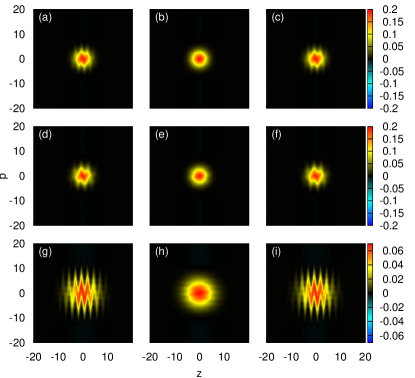
Figure 1: Wigner function for the quantum KHO for $q=4$, coupled to a heat bath (with $\beta=0.1$ and $D=5$), with an initial coherent state positioned at $z=0,p=0$. Different rows correspond to different choices of $\kappa$ and $\eta$. Resonant case (first row, $\kappa=-0.8,\eta^{2}=\pi$) after the 35’th kick (a), before the 36’th kick (b) and after the 36’th kick (c). Non-resonant case (second row, $\kappa=-0.8,\eta^{2}=0.7\,\pi$) at the same instances in time. Chaotic case (third row, $\kappa=-4.5,\eta^{2}=1$).

In Fig. 1 we present Wigner functions of an evolving quantum states, starting out at $\tau=0$ from the coherent state in the center of the phase space. We show the Wigner functions just after the 35’th kick (first row), right before the 36’th kick (second row) and right after the 36’th kick (third row). At these times, the system is already very close to its limit cycle behavior in all the cases, considered. This can be seen from Fig. 2, below. The main purpose of the figure is it to show that the limit cycle behavior is practically independent on the dynamical regime of the isolated KHO. The only quantity, which really matters is the kick amplitude $\kappa/(\sqrt{2}\,\eta^{2})$ from Eq. (6) which determines the amount of energy transfered to the system at each kick.

The first row shows the resonant case, with $\kappa=-0.8$ and $\eta^{2}=\pi$ such that the kick amplitude is $\kappa/(\sqrt{2}\,\eta^{2})\approx 0.18$. The second row shows the non-resonant case, with $\kappa=-0.8$ and $\eta^{2}=0.7\,\pi$, where $\kappa/(\sqrt{2}\,\eta^{2})\approx 0.25$. The third row shows the chaotic case, with $\kappa=-4.5$ and $\eta^{2}=1$, where $\kappa/(\sqrt{2}\,\eta^{2})\approx 3.18$. Remember, while $\kappa$ determines the degree of classical chaos in the system, $\eta$ is a scale factor which determines the size of classical structures on the phase space where quantum states occupy on average an area of size one. Thus, the semiclassical limit (usually denoted as $\hbar\to 0$) corresponds here to the limit $\eta^{2}\to\infty$.

Comparing the Wigner functions shown in the first and the second row, we can hardly note any differences. This confirms the dominant effect of the coupling to the heat bath. Without coupling, i.e. for the closed KHO, we would expect a much more extended Wigner function in the resonant case (here, the energy of the system increases quadratically in time) than in the non-resonant case (here, it increases only linearly). The Wigner functions in the third row correspond to the chaotic chase. There, the Wigner functions are much more extended. However, comparing the kick amplitudes calculated in the previous paragraph ($3.18$ for the chaotic case, vs. $0.18$ and $0.25$ for the resonant and non-resonant cases) we find that this larger extension is mainly due to the kick amplitude. The zig-zag pattern, most clearly recognizable for the states right after a kick can be directly related to the kick potential, as its periodicity in the z-direction agrees with that of the kick potential.

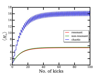
Figure 2: Energy of the harmonic oscillator $\langle H_{\mathrm{o}}\rangle$ vs. the number of kicks for the same three cases, shown in Fig. 1. The lowest curve (red line) corresponds to the resonant case with $\kappa=-0.8$ and $\eta^{2}=\pi$; the curve slightly above (green line) to the non-resonant case with $\kappa=-0.8$ and $\eta^{2}=0.7\,\pi$. The top curve (blue line) corresponds to the chaotic case with $\kappa=-4.5$ and $\eta^{2}=1$.

In Fig. 2, we show the evolution of the system energy $\langle H_{\mathrm{o}}\rangle$ as a function of the number of kicks, for the same three cases depicted in Fig. 1. Since $q=4$, the number of kicks which amount to one oscillator period (duration $2\pi$ in our dimensionless units) is equal to four. As we chose the same initial state (a coherent state at the origin), the energy of the system starts out at $\langle H_{\mathrm{o}}\rangle$. As can be seen from the figure, the evolution starts out at $\tau=0$ with a solution of the Caldeira-Leggett master equation. Since the energy of the system is smaller than the thermal energy of the heat bath, the system absorbs energy from the heat bath. Later on, the system energy will always be larger and the system will release energy to the heat bath. We observe that the two curves for the resonant and the non-resonant case are very close together, and they reach approximately the same final average energy, close to $D=5$. This means that the effect of the kicks is weak as compared to the heat bath. As a consequence, the limit cycle states are close to the thermal equilibrium state with $\langle H_{\mathrm{o}}\rangle=D=5$.

In the chaotic case (top most blue line), one can clearly observe the effect of each individual kick, and the subsequent relaxation. Here, the effect of the kicks is strong as compared to the heat bath. As a consequence, the average energy of the system is much larger than it would be due to the coupling to the heat bath alone. One may suspect that the limit cycle states vary around a thermal state with average energy close to $\langle H_{\mathrm{o}}\rangle=D=16$.

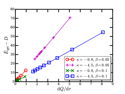
Figure 3: Difference between average system energy $\overline{E}_{\mathrm{qst}}$ from Eq. (17) vs. the heat current $\mathrm{d}Q/\mathrm{d}\tau$ from Eq. (18), for different KHO parameters $\kappa$ and $\eta^{2}$, as well as coupling strengths $\beta$; see legend. For each of the four cases, $\eta^{2}/\pi$ varies from $0.1$ to $1$ in integer steps. Larger values of $\eta^{2}$ mean smaller kick amplitudes, and hence the corresponding points are further away from the origin.

Let us now turn our attention to the energy balance in the quasi-stationary regime. Specifically, we consider the energy of the harmonic oscillator as a function of time, $E(\tau)=\langle H_{\mathrm{o}}\rangle$ at the time $\tau$. As far as time is concerned, we make use of the notation introduced in Sec. II.3 we denoted the time right after the $n$’th kick by $\tau_{n}^{+}=2\pi\,n/q+\delta$ with an infinitesimal increment $\delta$ (be reminded that time is measured in units such that one oscillator period is equal to $2\pi$). Similarly, we now denote $\tau_{n}^{-}$ as the time right before the $n$’th kick. The quasi-stationary regime may thus be characterized by the condition that the whole energy gained from any one kick, $E(\tau_{n}^{+})-E(\tau_{n}^{-})$ is subsequently transferred to the heat bath during the time interval $(\tau_{n}^{+},\tau_{n+1}^{-})$. For this regime, we hence introduce the average quasi-equilibrium energy of the oscillator as

$$\overline{E}_{\mathrm{qst}}=\lim_{n\to\infty}\frac{E(\tau_{n}^{+})+E(\tau_{n}^{-})}{2}\;.$$ (17)

On a coarse grained time scale of the order of many cycles, we may interpret the dynamics as a thermodynamic process where work (energy transfer due to the kicks) is continuously converted into heat, released to the reservoir. On the above mentioned coarse grained time scale, the heat flux from the oscillator to the heat bath is constant, and given by

$$\frac{\mathrm{d}Q}{\mathrm{d}\tau}=\frac{q}{2\pi}\;\lim_{n\to\infty}\big{[}E(\tau_{n}^{+})-E(\tau_{n+1}^{-})\big{]}\;.$$ (18)

In Fig. 3, we study the amount of heat transfered to the reservoir as a function of the energy difference $\overline{E}_{\mathrm{qst}}-D$, which may be interpreted as a temperature difference between the heat bath and the oscillator. This assumes that it is possible to assign a temperature to the oscillator in this quasi- equilibrium situation. One then expected that the Fourier law (of thermal conduction) would hold, which predicts a linear relation between both quantities. Indeed, Fig 3 seems to confirm the validity of the Fourier law.

III.2 Weak coupling and reappearance of quantum chaotic/resonance properties

In the previous Sec. III.1, we studied the case of strong coupling to the heat bath, where different dynamically properties of the quantum KHO almost do not play any role. It is then natural to ask, at which scales and how the different dynamical features re-appear, when the coupling to the heat bath is reduced. This is the purpose of the present section.

For the KHO, we have essentially three different parameters which can be changed, (i) the kick period $\tau_{n+1}-\tau_{n}=2\pi/q$, which may or may not be commensurable with the period $2\pi$ of the harmonic oscillator; (ii) the scale-invariant kick strength $\kappa$, which determines the degree of chaos in the corresponding classical system; and (iii) the scale (size) of the system in phase space, which is determined by $\eta$. As mentioned earlier, taking $\eta\to\infty$ implements the semiclassical limit. However, $\eta$ is also the parameter which controls the quantum resonances, as it happens that for specific integer values of $q$, the system energy can increase quadratically in time, whereas otherwise it only increases linearly. For small coupling $\beta$, the study of the system is limited to a relatively narrow range of parameters or to short times. This is because, our numerical scheme starts to fail if the Wigner functions become too extended in phase space. In those cases, it is increasingly difficult to reach the quasi-stationary regime.

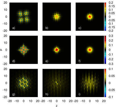
Figure 4: Wigner function for the KHO coupled to heat bath, right after the 36’th kick, for different coupling strengths: $\beta=0.001$ (first column), $\beta=0.01$ (second column), and $\beta=0.1$ (third column). Again we consider three cases, the resonant case (first row) with $\kappa=-0.8$ and $\eta^{2}=\pi$; the non-resonant case (second row) with $\kappa=-0.8$ and $\eta^{2}=(1+\sqrt{5})\,\pi/2$ (resonant cases is considered in the Figs. 1 and 2). The chaotic case (third row) with $\kappa=-4.5$, $\eta^{2}=1$, however has a different inter-kick period, with $q=6$.

In Fig. 4 we show Wigner functions after the 36’th kick. Similar to Fig. 1, we consider the resonant, non-resonant and chaotic case, each case in a different column. However, we now vary the coupling strength from $\beta=0.001$ (first column) to $\beta=0.01$ (second column), and $\beta=0.1$ (third column). The cases shown in the third column agree with those shown in Fig. 1, except for the chaotic case, where we chose $q=6$ instead of $q=4$. In this case, where $\beta$ is sufficiently large, the quasi-stationary regime is almost reached, and we can observe some minor differences between the $q=6$ and $q=4$ case. For small values of $\beta$ (first column), we find regions where the Winger function becomes negative. This is a clear signature for the state to be non-classical. For $\beta=0.001$ and $0.01$, we also observe that the extension of the Wigner function is larger for the resonant case than for the non-resonant case, as expected according to the quadratic over linear energy absorption. As shown in Fig. 2, this is no longer the case for $\beta=0.1$, where the quantum resonance condition seems to become meaningless. In the chaotic case, the extension of the Wigner function is by far largest. However, as explained in Fig. 1, this is a simple consequence of the large kick amplitude. In the chaotic case, one would expect a linear increase in energy, just as in the non-resonant case  Kells et al. (2004). Note that the hexagonal symmetry observable for $\beta=0.001$, which is due to the choice of $q=6$, disappears as $\beta$ is increased, until at $\beta=0.1$ the characteristic zig-zag shape appears, similar to the $q=4$ case, shown in Fig. 1.

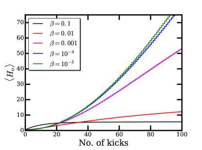
Figure 5: Energy evolution in time in the resonant case, $q=4,\kappa=-0.8,\eta^{2}=\pi$ for different coupling strengths, from $\beta=10^{-5}$ (green line) to $\beta=0.1$ (black line).

In Fig. 5 the expectation value of the oscillator energy is shown as a function of the number of kicks applied to the system. The parameters for the KHO ($q=4,\kappa=-0.8,\eta^{2}=\pi$) are chosen to be the same as for one of the two resonant cases shown in Fig. 3(b) of Ref. Billam and Gardiner (2009), where the quantum KHO is treated without dissipation. Indeed, our result for $\beta=10^{-5}$ seems to agree very well with the result shown there. We can clearly see the quadratic increase in energy, which becomes only slightly diminished when $\beta$ is increased to $\beta=10^{-4}$. By contrast, for the largest coupling, $\beta=0.1$, the energy only increases in an initial phase, and then quickly approaches its limit (average) value of $\langle H_{\mathrm{o}}\rangle=D=5$. For intermediate couplings, $\beta=0.001$ and $\beta=0.01$, the increase of the energy is no longer quadratic, but the quasi stationary regime only sets in after many more kicks than could be shown here.

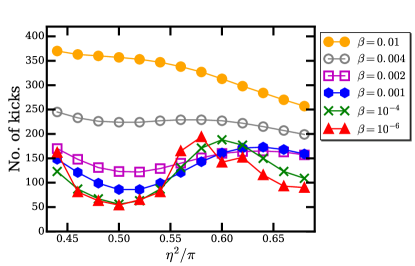
Figure 6: Plots of the number of kicks required to reach a mean energy of $50\hbar\omega$ for the resonant case (with $\kappa=-0.8$, $q=4$) and different coupling strength values, $\beta$; the resonance is in $\eta^{2}/\pi=0.5$.

In Fig. 6 we plot the number of kicks required to reach the energy of $\langle H_{\mathrm{o}}\rangle=50$ (in units of $\hbar\omega_{\mathrm{o}}$). Again, this is done for the resonant case, with $q=4$, $\kappa=-0.8$. This time $\eta$ is varied in a small region around the quantum resonance condition $\eta^{2}=\pi/2$. This corresponds to the second case of a quantum resonance, also considered in Ref. Billam and Gardiner (2009). For $\eta^{2}$, we focus on a small section from a similar figure from that reference. Now, we plot the number of kicks required to reach the above mentioned energy limit, as a function of $\eta^{2}$ for different coupling strengths, from $\beta=10^{-6}$ to $\beta=0.01$. For the smallest coupling strength, we find the expected minimum, and we again confirm a good agreement with the corresponding result in Fig. 3(a) from Ref. Billam and Gardiner (2009). For increasing $\beta$, the minimum remains at its place, approximately until $\beta=0.002-0.004$, and then disappears. At the largest coupling, $\beta=0.01$, the number of kicks required to reach the energy limit becomes a monotonous function of $\eta^{2}$. It is noteworthy that increasing the coupling from $\beta=10^{-6}$ to $\beta=10^{-5}$ already leads to notable differences, but only sufficiently far away from the quantum resonance. It is also interesting that for fixed $\eta^{2}\approx 0.0575\pi$, the number of kicks required does not increase monotonously with $\beta$. This phenomenon of increasing energy absorption due to increasing the coupling to a heat bath might be related to destroying a dynamical localization effect by increasing decoherence Frasca (1997); Kells et al. (2004).

IV Conclusions

In this paper, we described the quantum kicked harmonic oscillator as an open quantum system coupled to a finite temperature heat bath. We studied its equilibrium properties at relatively strong coupling, and found that there, the system fulfills fundamental thermodynamic properties such as the Fourier law for heat transport. When reducing the coupling to the heat bath, the system’s equilibrium state (i.e. its Wigner function representation) becomes ever more extended in phase space, and the expectation value of the oscillator energy increases. This makes it ever more difficult to perform simulations for a long time (many kicks), and eventually we are no longer able to reach the equilibrium state. Thus, for small coupling, we restrict ourselves to study the effect of quantum resonances and how it becomes suppressed and eventually eliminated due to the increasing coupling to the heat bath.

The numerical method is limited essentially by the requirement of an accurate representation of the chord function. At the present stage, we use a simple uniform two dimensional grid together with bilinear interpolation Press (1992). However, we are confident to be able to improve that scheme in order to be able to reach higher energies and larger times.

As shown in Ref. Lemos et al. (2012) the model is realizable experimentally in an quantum optical setup. Alternatively one might think of ions in a harmonic trap. The coupling of the ion movement to its internal electronic states opens a way to consider the KHO with heat bath as the environment for a central quantum system, which may serve as a probe for the thermodynamical properties of KHO.

Appendix A Solution of the Caldeira-Leggett master equation for the quantum harmonic oscillator

The Caldeira-Leggett master equation for the harmonic oscillator transformed into the chord function representation in the dimensionless variables description reads:

$$\partial_{\tau}\mathrm{w}+(\beta s-k)\partial_{s}\mathrm{w}+s\partial_{k}\mathrm{w}=-D\beta s^{2}\mathrm{w}$$ (19)

where $\mathrm{w}=\mathrm{w}(\vec{r},\tau)$ and $\vec{r}=(k,s)$. This is a first order partial differential which can be solved by standards procedures. The equation (12) can be written in its parametric form: equation in the parametric form is

$$\frac{\mathrm{d}s}{\mathrm{d}\tau}=\beta s-k,\quad\frac{\mathrm{d}k}{\mathrm{d}\tau}=s,\quad\frac{\mathrm{d}}{\mathrm{d}\tau}\mathrm{w}(\vec{r},\tau)=-D\beta s^{2}\mathrm{w}(\vec{r},\tau).$$ (20)

By coupling the first two set of equations, one has the solution for the case $\beta<1$:

$$k_{\tau} = u_{1}(\tau)a_{1}+u_{2}(\tau)a_{2}$$ (21)

$$s_{\tau} = u_{3}(\tau)a_{1}+u_{4}(\tau)a_{2}$$ (22)

where we have called for simplicity

$$u_{1}(\tau)=\mathrm{e}^{\beta\tau\over 2}\sin\omega\tau, \quad u_{2}(\tau)=\mathrm{e}^{\beta\tau\over 2}\cos\omega\tau$$ (23)

$$u_{3}(\tau)=\frac{\mathrm{d}}{\mathrm{d}\tau}u_{1}(\tau), \quad u_{4}(\tau)={\mathrm{d}\over\mathrm{d}\tau}u_{2}(\tau),$$ (24)

with $\omega=\sqrt{1-\beta^{2}/4}$. The constants $a_{1}$ and $a_{2}$ are known as the characteristics curves and they emerge as integration constants of the solution of the first two set of equations in (20). In terms of them, the map of any set of points $k$ and $s$ at the time $\tau$ described in terms of the characteristics: $k=u_{1}(\tau)a_{1}+u_{2}(\tau)a_{2}$ and $s=u_{3}(\tau)a_{1}+u_{4}(\tau)a_{2}$ to the points $k^{\prime}$ and $s^{\prime}$ at the time $\tau+\sigma$, is done by moving along the characteristic curves. This map can be represented by the following transformation:

$$\vec{r}_{\tau+\sigma}=\bm{M}(\sigma)\;\vec{r}_{\tau}$$ (25)

where the matrix $\bm{M}(\sigma)$ has the form:

$$\bm{M}(\sigma)=\mathrm{e}^{\beta\sigma/2}\left(\begin{array}[]{cc}m_{1}(\sigma)&m_{2}(\sigma)\\ m_{3}(\sigma)&m_{4}(\sigma)\end{array}\right)$$ (26)

and

$$m_{1}(\sigma) = \cos\omega\sigma-{\beta\over 2\omega}\sin\omega\sigma,$$ (27)

$$m_{2}(\sigma) = {1\over\omega}\sin\omega\sigma,$$ (28)

$$m_{3}(\sigma) = {-1\over\omega}\sin\omega\sigma,$$ (29)

$$m_{4}(\sigma) = \omega\cos\omega\sigma+{\beta\over 2}\sin\omega\sigma.$$ (30)

The mapping is reversible as one can check that the relations $\bm{M}(\sigma)^{-1}=\bm{M}(-\sigma)$ holds. The matrix $\bm{M}(\cdot)$ is also composed by a rotational and contracting part, so as the maps goes to infinity, the characteristics moves any initial set of points into the origin. Integration of the third equation of (20) is of the form

$$\int_{\mathrm{w}(\tau)}^{\mathrm{w}(\tau+\sigma)}{\mathrm{d}\mathrm{w}\over\mathrm{w}}=-D\beta\int_{\tau}^{\tau+\sigma}\mathrm{d}\tau^{\prime}\,s^{2}(\tau^{\prime}).$$ (31)

where $\mathrm{w}(\tau)=\mathrm{w}(\vec{r},\tau)$ is the initial condition of the oscillator whose dependence on the variables $k$ and $s$ at $\tau$. By using the relation of the characteristics (21) and (22) one can write the argument of the integral in the r.h.s of (31) in terms of the variables $k$ and $s$ at time $\tau$ as: $s(\tau^{\prime})=\mathrm{e}^{-{\beta\over 2}{\left(\tau-\tau^{\prime}\right)}}\left(m_{3}(\tau-\tau^{\prime})k+m_{4}(\tau-\tau^{\prime})s\right)$ and perform the integration yielding the solution for the chord function at the time $\tau+\sigma$:

$$\mathrm{w}(\vec{r},\tau+\sigma)=\mathrm{w}\left(\,\bm{M}(-\sigma)\;\vec{r},\,\tau\,\right)\mathrm{e}^{-D\beta\left[\,\vec{r}^{T}\,\bm{A}(\sigma)\,\vec{r}\,\right]}$$

where the matrix $\bm{A}(\sigma)$ depends also on the time of propagation from the initial condition to the final time and has the form:

$$\bm{A}(\sigma)=\left(\begin{array}[]{cc}A_{1}(\sigma)&A_{2}(\sigma)\\ A_{2}(\sigma)&A_{3}(\sigma)\end{array}\right),$$ (32)

and

$$A_{1}(\sigma) = \int_{0}^{\sigma}\mathrm{d}\tau^{\prime}\,\mathrm{e}^{\beta\tau^{\prime}}m^{2}_{3}(-\tau^{\prime})$$ (33)

$$A_{2}(\sigma) = \int_{0}^{\sigma}\!\!\mathrm{d}\tau^{\prime}\,\mathrm{e}^{\beta\tau^{\prime}}\!m_{3}(-\tau^{\prime})m_{4}(-\tau^{\prime})$$ (34)

$$A_{3}(\sigma) = \int_{0}^{\sigma}\mathrm{d}\tau^{\prime}\,\mathrm{e}^{\beta\tau^{\prime}}m^{2}_{4}(-\tau^{\prime}).$$ (35)

Appendix B The stationary state of the quantum harmonic oscillator in the Caldeira-Leggett model

As the system propagates in contact with the thermal bath, the system relaxes into a thermal stationary state correspondent to the Caldeira-Leggett model for which the high temperature limit is assumed. The form of the stationary state can be obtained by taking the long time limit $\sigma\rightarrow\infty$ in the solution of the master equation in the chord function description (A). In this limit, $\lim_{\sigma\rightarrow\infty}\,\bm{M}(-\sigma)=0$. If one assumes in a general context an initial condition for the system as coherent state: $\psi(X)=({m\omega_{\mathrm{o}}\over\pi\hbar})^{1/4}\mathrm{e}^{\mathrm{i}P_{\mathrm{o}}X-{m\omega_{\mathrm{o}}\over 2\hbar}(X-X_{\mathrm{o}})^{2}}$ which in the chord function representation the initial condition takes the form:

$$\mathrm{w}\left(\vec{r},\tau\right)=\sqrt{m\omega_{\mathrm{o}}\over 2\pi\hbar}\,\mathrm{e}^{\mathrm{i}{P_{\mathrm{o}}\over k_{\mathrm{o}}}s+\mathrm{i}X_{o}k-{k^{2}\over 4}-{s^{2}\over 4}},$$ (36)

then in the long time limit, the dependence of the system on the state of the initial condition vanishes, yielding only a constant term:

$$\lim_{\sigma\rightarrow\infty}\mathrm{w}\left(\,\bm{M}(-\sigma)\;\vec{r},\,\tau\,\right)=\sqrt{m\omega_{\mathrm{o}}\over 2\pi\hbar}.$$ (37)

On the other hand the form of the $\bm{A}(\sigma)$ matrix as $\sigma\rightarrow\infty$ is:

$$\lim_{\sigma\rightarrow\infty}\bm{A}(\sigma)={1\over 2\beta}\left(\begin{array}[]{cc}1&\beta\\ \beta&1+\beta^{2}\end{array}\right),$$ (38)

which in the limit of applicability of the Born-Markov approximation, $\beta\ll\pi D$, which is an assumption of the derivation of the Caldeira-Leggett master equation, the $\bm{A}(\sigma\rightarrow\infty)$ matrix can be approximated to ${1\over 2\beta}\openone$, where $\openone$ is the $2\times 2$ unit matrix. The chord function at the stationary regime can be written as:

$$\mathrm{w}(\vec{r},\sigma\rightarrow\infty)=\sqrt{m\omega_{\mathrm{o}}\over 2\pi\hbar}\mathrm{e}^{-{D\over 2}\left(k^{2}+s^{2}\right)}$$

Transformation of the chord function (B) into the position representation yields the following density matrix for the stationary regime:

$$\varrho_{\mathrm{ths}}(X,X^{\prime})=\sqrt{m\omega_{\mathrm{o}}^{2}\over 2\pi k_{B}T}\mathrm{e}^{-{m\omega_{\mathrm{o}}^{2}\over 8k_{B}T}(X+X^{\prime})^{2}-{mk_{B}T\over 2\hbar^{2}}\left(X-X^{\prime}\right)^{2}},$$ (39)

which agrees with the solution for the Caldeira-Legget master equation for the stationary regime, see e.g. Ramazanoglu (2009); Breuer and Petruccione (2002) The average energy of the system at the stationary regime becomes exactly $E_{\mathrm{therm}}=\langle H_{\mathrm{osc}}\rangle=k_{B}T$ as in a thermalization process. The role of $\beta$, is related to the rapidity of the relaxation process into the thermal state. The Wigner function of the system at the thermal state has the following form:

$$\mathrm{W}_{\mathrm{ths}}(z,p)=\sqrt{\frac{m\omega_{\mathrm{o}}}{2\pi\hbar D^{2}}}\;\exp\!\Big{(}-\frac{z^{2}+p^{2}}{2D^{2}}\Big{)}\;,$$ (40)

which is a Gaussian function centered at the origin with standard deviation $D$.

References

- Gemmer et al. (2009) J. Gemmer, M. Michel, and G. unter Mahler, Quantum Thermodynamics: Emergence of thermodynamic behavior within composite quantum systems, 2nd ed., Lecture notes in physics, Vol. 784 (Springer Verlag Berlin Heidelberg, Berlin, Heidelberg, 2009).
- Stöckmann (1999) H.-J. Stöckmann, quantum chaos (Cambridge University Press, Cambridge, UK, 1999).
- Haake (2001) F. Haake, Quantum signatures of chaos, 2nd. Edition (Springer, Berlin, Heidelberg, 2001).
- Srednicki (1994) M. Srednicki, Phys. Rev. E 50, 888 (1994).
- Cohen (1997) D. Cohen, Phys. Rev. Lett. 78, 2878 (1997).
- Berry and Tabor (1977) M. V. Berry and M. Tabor, Proc. R. Soc. Lond. A 356, 375 (1977).
- Casati et al. (1980) G. Casati, F. Valz-Gris, and I. Guarneri, Lett. Nuovo Cimento 28, 279 (1980).
- O. Bohigas and Schmit (1995) A. M. O. d. A. O. Bohigas, M.-J. Giannoni and C. Schmit, Nonlinearity 8, 203 (1995).
- Blümel and Smilansky (1990) R. Blümel and U. Smilansky, Phys. Rev. Lett. 64, 241 (1990).
- Lutz and Weidenmüller (1999) E. Lutz and H. A. Weidenmüller, Physica A 267, 354 (1999).
- Esposito and Gaspard (2004) M. Esposito and P. Gaspard, EPL (Europhysics Letters) 65, 742 (2004).
- Gorin and Seligman (2002) T. Gorin and T. H. Seligman, J. Opt. B: Quantum Semiclass. Opt. 4, S386 (2002), topical issue: Mysteries and Paradoxes in Quantum Mechanics IV Quantum interference phenomena (Workshop held at Gargano, Italy, August 2001).
- Gorin and Seligman (2003) T. Gorin and T. H. Seligman, Phys. Lett. A 309, 61 (2003).
- Pineda et al. (2007) C. Pineda, T. Gorin, and T. H. Seligman, New Journal of Physics 9, 106:1 (2007).
- Gorin et al. (2008) T. Gorin, C. Pineda, H. Kohler, and T. H. Seligman, New Journal of Physics 10, 115016 (2008).
- David (2011) F. David, Journal of Statistical Mechanics: Theory and Experiment 2011, P01001 (2011).
- Carrera et al. (2014) M. Carrera, T. Gorin, and T. H. Seligman, Phys. Rev. A 90, 022107 (2014).
- Gelbart et al. (1972) W. M. Gelbart, S. A. Rice, and K. F. Freed, The Journal of Chemical Physics 57, 4699 (1972).
- Caldeira and Leggett (1983) A. O. Caldeira and A. J. Leggett, Physica 121A, 587 (1983).
- Breuer and Petruccione (2002) H.-P. Breuer and F. Petruccione, The Theory of open quantum systems (Oxford University Press, 2002).
- Ramazanoglu (2009) F. M. Ramazanoglu, Journal of Physics A: Mathematical and Theoretical 42, 265303 (2009).
- Chernikov et al. (1988) A. Chernikov, R. Sagdeev, and G. Zaslavsky, Physica D: Nonlinear Phenomena 33, 65 (1988).
- Reichl (1992) L. E. Reichl, “Global properties,” in The Transition to Chaos: In Conservative Classical Systems: Quantum Manifestations (Springer New York, New York, NY, 1992) pp. 156–221.
- Zaslavsky (2002) G. Zaslavsky, Physics Reports 371, 461 (2002).
- Gardiner et al. (1997) S. A. Gardiner, J. I. Cirac, and P. Zoller, Physical Review Letters 79, 4790 (1997).
- Carvalho et al. (2004) A. R. R. Carvalho, R. L. de Matos Filho, and L. Davidovich, Phys. Rev. E 70, 026211 (2004).
- Billam and Gardiner (2009) T. P. Billam and S. A. Gardiner, Phys. Rev. A 80, 023414 (2009).
- Kells et al. (2004) G. A. Kells, J. Twamley, and D. M. Heffernan, Phys. Rev. E 70, 015203 (2004).
- Lemos et al. (2012) G. B. Lemos, R. M. Gomes, S. P. Walborn, P. H. Souto Ribeiro, and F. Toscano, Nat Commun 3, 1211 (2012).
- Ketzmerick and Wustmann (2010) R. Ketzmerick and W. Wustmann, Phys. Rev. E 82, 021114 (2010).
- Langemeyer and Holthaus (2014) M. Langemeyer and M. Holthaus, Phys. Rev. E 89, 012101 (2014).
- de Almeida (1998) A. M. O. de Almeida, Physics Reports 295, 265 (1998).
- de Almeida (2003) A. M. O. de Almeida, Journal of Physics A: Mathematical and General 36, 67 (2003).
- Ángel Prado Reynoso (2016) M. A. Prado, Dinámica en el espacio de fase del oscilador armónico pateado acoplado a un entorno térmico, Master’s thesis, Universidad de Guadalajara (2016).
- Frasca (1997) M. Frasca, Physics Letters A 231, 344 (1997).
- Roy and Venugopalan (1999) S. M. Roy and A. Venugopalan, “Exact solutions of the caldeira-leggett master equation: A factorization theorem for decoherence,” arXiv: quant-ph/9910004 (1999).
- Abramowitz and Stegun (1970) M. Abramowitz and I. A. Stegun, eds., Handbook of mathematical functions (Dover publications, inc., New York, 1970).
- Press (1992) W. H. Press, ed., Numerical recipes in Fortran (Cambridge University Press, 1992).