A Benchmark Test of Boson Sampling on Tianhe-2 Supercomputer

Abstract

Boson sampling, thought to be intractable classically, can be solved by a quantum machine composed of merely generation, linear evolution and detection of single photons. Such an analog quantum computer for this specific problem provides a shortcut to boost the absolute computing power of quantum computers to beat classical ones. However, the capacity bound of classical computers for simulating boson sampling has not yet been identified. Here we simulate boson sampling on the Tianhe-2 supercomputer which occupied the first place in the world ranking six times from 2013 to 2016. We computed the permanent of the largest matrix using up to 312,000 CPU cores of Tianhe-2, and inferred from the current most efficient permanent-computing algorithms that an upper bound on the performance of Tianhe-2 is one 50-photon sample per $\sim$100 min. In addition, we found a precision issue with one of two permanent-computing algorithms.

I Introduction

Universal quantum computers promise to substantially outperform classical computers Deutsch1997 ; Nielsen2011 . However, building them has been experiencing challenges in practices, due to the stringent requirements of high-fidelity quantum gates and scalability. For example, Shor’s algorithm Shor1994 , which solves the integer factorization problem, is one of the most attractive quantum algorithms because of its potential to crack current mainstream RSA cryptosystems. The key size crackable on classical computers is 768 bits Kleinjung2010 . This size, however, requires millions of qubits for a quantum computer to do the factorization Fowler2012 , far from current technology Martin2012 ; Lanyon2007 ; Politi2009 ; Parker2000 ; Lu2007 ; Monz2016 ; Vandersypen2001 . This gap motivates research into purpose-specific quantum computation with quantum speedup and more favorable experimental conditions.

Boson sampling Aaronson2011 is a specific quantum computation thought to be an outstanding candidate for beating the most powerful classical computer in the near term. It samples the distribution of bosons output from a complex interference network. Unlike universal quantum computation, quantum boson-sampling seems to be more straightforward, since it only requires identical bosons, linear evolution and measurement. As for classical computers, the distribution can be obtained by computing permanents of matrices derived from the unitary transformation matrix of the network Scheel2008 , in which the most time-consuming task for the simulation of boson sampling is the calculation of permanents. However, computing the permanent has been proved as a #P-hard task on classical computers Aaronson2011 . This motivates massive advances in building larger quantum boson-sampling machines to outperform classical computers, including principle-of-proof experiments Spring2013 ; Broome2013 ; Tillmann2013 ; Crespi2013 , simplified models that are easy to implement Aaronson2013blog ; Lund2014 ; Bentivegnae2015 , implementation techniques Motes2014 ; Spring2016 ; Carolan2015 ; Defienne2016 , robustness of boson sampling Rohde2012err ; Rohde2012 ; Rahimi2016 ; Motes2013 ; Motes2015 , validation of large scale boson sampling Aaronson2014 ; Spagnolo2014 ; Wang2016 , varied models for other quantum states Rohde2015 ; Seshadreesan2015 ; Olson2015 , etc.

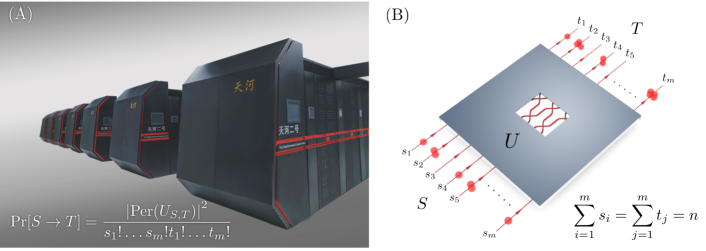
Figure 1: A schematic view of computational task with the Tianhe-2 supercomputer (A) and a quantum boson-sampling machine (B). A quantum boson-sampling machine obtains an $n$-photon sample $T$ directly through a measurement on the $m$ output ports from the network that described by a unitary matrix $U$ with input $S$. To simulate the generation of a sample on Tianhe-2, it is necessary to compute the probability $\text{Pr}[S\rightarrow T]$, in which the main time-consuming task is to calculate the permanent of an $n\times n$ sub-matrix $U_{S,T}$ of $U$. The capacity of computing the permanent on Tianhe-2 is employed to benchmark the state of the art and set an upper bound on the classical execution time to be beaten by quantum boson-sampling machine.

However, what is the capacity bound of a state-of-the-art classical computer for simulating boson sampling? This bound indicates the condition on which a quantum boson-sampling machine will surpass classical computers.

Given an $m\times m$ unitary matrix $U$ and $n$ indistinguishable bosons (as shown in FIG. 1(B)), the simulation on classical computers is to generate samples from the output distribution described by Equation (1).

$$\text{Pr}[S\rightarrow T]=\frac{\left|\text{Per}(U_{S,T})\right|^{2}}{s_{1}!\ldots s_{m}!t_{1}!\ldots t_{m}!}$$ (1)

where $S=|s_{1},\ldots,s_{m}\rangle$ is a given input state with $s_{i}$ bosons in the $i^{\text{th}}$ input port, $T=|t_{1},\ldots,t_{m}\rangle$ is an output state with $t_{j}$ bosons in the $j^{\text{th}}$ output port, and $U_{S,T}$ is an $n\times n$ sub-matrix derived from $U$ Aaronson2011 . The permanent calculation is the most time-consuming task in the simulation of boson sampling on a classical computer, because it is the source of the hardness in the complexity conjecture Aaronson2011 . Therefore, the performance of computing the permanent of the $n\times n$ sub-matrix, $U_{S,T}$, is an upper bound on the performance of generating an $n$-photon sample from the distribution $\text{Pr}[S\rightarrow T]$. In this paper, we evaluate this upper bound by testing two most efficient permanent-computing algorithms on the Tianhe-2 supercomputer Liao2014 (FIG. 1(A)). The results show that Tianhe-2 requires about 100 min to generate one 50-photon sample.

II Speed Performance

The two most efficient permanent-computing algorithms, Ryser’s algorithm and BB/FG’s algorithm, are both in the time complexity of $O(n^{2}\cdot 2^{n})$.

We implemented Ryser’s algorithm and BB/FG’s algorithm (see the supplementary material for details), and ran them on the Tianhe-2 supercomputer. This supercomputer consists of 16,000 computing nodes, each containing three CPUs and two co-processors, denoted as MIC. The programs were tested under two types of configurations: running with only CPUs, or hybrid running with both CPUs and MICs.

We ran Ryser’s algorithms with the number of nodes ranging from 2,048 to 13,000, as shown in TABLE 1. It is difficult for a system of very large scale to complete long-running-time execution, because the system reliability becomes worse as the number of processing units increases Yang2012 . Occasionally, slow nodes would prolong the total execution time. This phenomenon can be seen from the data in TABLE 1, since the time used is not reduced in proportion (more specifically, the time used for a $46\times 46$ permanent using 4,096, 8,192 and 13,000 nodes). Up to now, the $48\times 48$ matrix’s permanent is the largest problem computed on 8,192 nodes, which accounts for more than half of the nodes of Tianhe-2, and the 13,000-node test uses 81.25% CPUs of Tianhe-2, the largest amount of computing resources ever, for the boson-sampling problem.

Table 1: Large-scale tests of Ryser’s algorithm on the Tianhe-2 supercomputer. Each row of the table gives the result of testing an $n\times n$ matrix with $C$ CPU cores of $P$ computing nodes. Items in “Predicted time (s)” column are intervals of predicted execution time through fitting results of tests on the subsystem. The red items show that the execution time is longer than expected, suggesting the existence of slow nodes.

$n$	$P$	$C$	Execution time (s)	Predicted time (s)
40	4,096	98,304	24.863563	[22.650, 27.758]
40	8,192	196,608	14.105145	[11.076, 13.726]
45	2,048	49,152	1967.7603	[1875.8, 2273.5]
45	4,096	98,304	984.02218	[917.34, 1124.2]
45	4,096	98,304	981.25833	[917.34, 1124.2]
45	4,096	98,304	986.09726	[917.34, 1124.2]
45	4,096	98,304	981.44862	[917.34, 1124.2]
45	13,000	312,000	450.62642	[278.54, 347.72]
46	4,096	98,304	2096.3798	[1917.1, 2349.4]
46	8,192	196,608	1054.9386	[937.54, 1161.7]
46	13,000	312,000	1034.0247	[582.13, 726.71]
48	8,000	192,000	4630.0842	[4184.5, 5183.4]
48	8,000	192,000	4628.1068	[4184.5, 5183.4]
48	8,000	192,000	4657.8987	[4184.5, 5183.4]
48	8,000	192,000	4648.9111	[4184.5, 5183.4]
48	8,000	192,000	4627.6037	[4184.5, 5183.4]
48	8,192	196,608	4530.5931	[4083.3, 5060.0]
48	8,192	196,608	4498.4557	[4083.3, 5060.0]

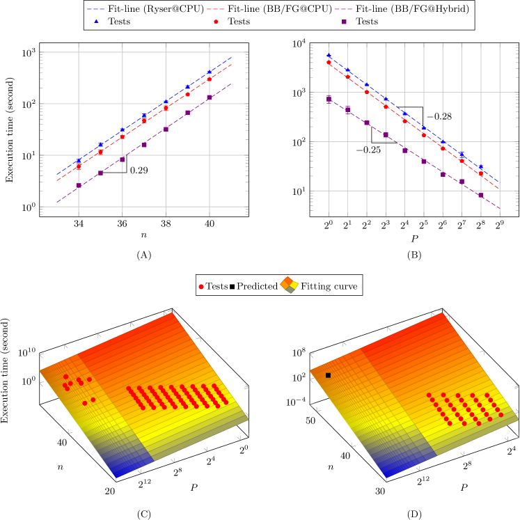
Figure 2: Scalability. (A) and (B) show the execution time for $P$ nodes to compute the permanent of an $n\times n$ matrix. The “@CPU” terms are the results obtained from the running only on CPUs, and the “Hybrid” terms are the execution time on CPUs accelerated with co-processors. The slope of the fit-lines indicates the execution time increase by $\sim$$1.95$ times when $n$ increases by 1, and decrease by $0.52\sim 0.56$ times when the number of computing nodes doubles. The error bars, where visible, denote one standard deviation. (C) is the fitted execution time of Ryser’s algorithm for $P$ nodes to compute the permanent of an $n\times n$ matrix. The adjusted R-square statistic is 0.9996, indicating a good fit. (More details are given in the supplementary material.) (D) is the fitted execution time of BB/FG’s algorithm. The black point is the predicted time used for the full system of Tianhe-2 to compute the permanent of a $50\times 50$ matrix.

Both the algorithms were tested on a 256-node subsystem of Tianhe-2 (which still has a theoretical peak performance of 848.4 teraflops, which may be ranked in top 160 in the Top500 list in November 2015) to evaluate the scalability through tests under different parameter combinations of matrix order and number of the parallel scale. As shown by the results in FIG. 2, execution time increases by $\sim$1.95($\approx 10^{0.29}$) times when $n$ increases by 1 (part A), and decreases with a nearly linear speedup when the number of nodes used increases (part B). These results reflect the fact that our programs are very scalable with only a little extra cost from the parts that cannot be parallelized.

To evaluate the scalability in more detail, we propose a fitting equation of the execution time involving both problem size and computing resources, as shown in Equation (2).

$$T=\frac{an^{2}2^{n}}{P^{b}}$$ (2)

where $a$ and $b$ are the fitting coefficients, and $T$ represents the execution time of computing the permanent of an $n\times n$ matrix with $P$ computing nodes. We fitted the execution time of Ryser’s algorithm with data tested on $1$ to $13,000$ nodes, as shown in FIG. 2(C). The fitted $b$ is $0.9924$, showing the good scalability of our programs again. This comes from the feature of the algorithm. The amount of communication is just $O(n^{2}P)$, while that of computation is $O(n^{2}2^{n})$, growing much faster than that of communication.

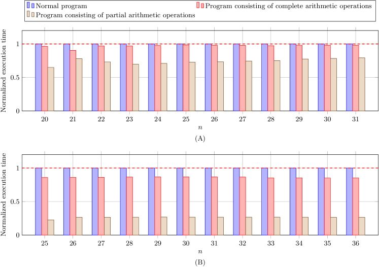
Figure 3: Efficiency for utilizing CPUs and co-processors. (A) and (B) are normalized execution time on CPUs and co-processors respectively. The ratios of the execution time of the two modified programs over that of normal ones are considered as efficiency. The average efficiency for CPUs is 97.0% and 74.0% following the order in the figure, and that for co-processors is 86.0% and 26.3%.

To evaluate the efficiency at which our programs utilize CPUs and co-processors, we removed implementation-related instructions from our programs, only leaving essential arithmetic operations connected to the computational complexity. The execution time of this kind of program is viewed as a baseline. FIG. 3 shows that our programs have exploited the performance from CPUs and co-processors in considerable efficiency. More evaluations and further analysis can be found in the supplementary material.

We used the fitted execution time of BB/FG’s algorithm, not that of Ryser’s due to its precision issue (discussed in the next section), to analyze the capacity bound of the full system of Tianhe-2. The fitting equation is shown in Equation (3).

$$T=\frac{9.805\cdot n^{2}2^{n}}{P^{0.8782}\times 10^{12}}$$ (3)

The fitting result, in FIG. 2(D), suggests that the execution time for the full system of Tianhe-2 with all CPUs and co-processors to compute the permanent of a $50\times 50$ matrix would be about 93.8 min, while the 95% confidence bound of this prediction is [77.41, 112.44] min, which means that an upper bound of Tianhe-2 is one 50-photon sample per $\sim$100 min.

III Precision Performance

A precision issue was found during the test of Ryser’s algorithm. The limited word length of classical electricity computers leads to an accumulated rounding error (see supplementary material for details). To evaluate the errors of the two algorithms, a special type of matrix, an all-ones matrix, was used for its theoretical value is easy to obtain. The result reveals that, as shown in FIG. 5, the relative error of Ryser’s algorithm reaches nearly 100% when $n\geq 30$.

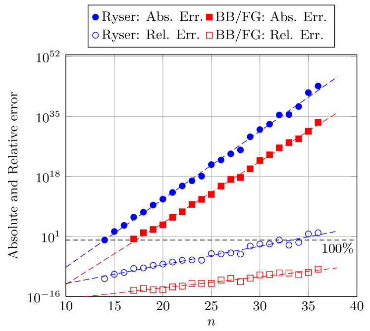
Figure 4: Errors of computing permanents of $n\times n$ all-ones matrices. An absolute error for a permanent of the $n\times n$ all-ones matrix is the substraction between the computed value and the theoretical value ($n!$). Both the errors of Ryser’s algorithm and BB/FG’s algorithm grow exponentially with the increase of $n$. The relative errors are computed through dividing the absolute errors by the theoretical values. Unfortunately, the relative error rate of Ryser’s algorithm for a $32\times 32$ all-ones matrix reaches beyond 100%.

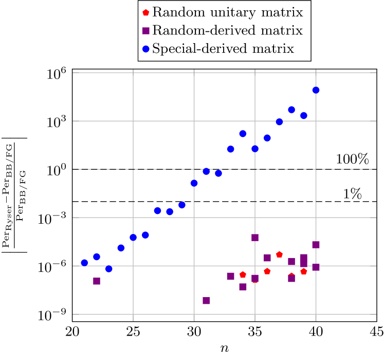
Figure 5: Errors of computing permanents of $n\times n$ random matrices. “Random unitary matrix” denotes results of matrices corresponding to that each input (output) port of an interference network injecting (ejecting) one and only one boson. “Random-derived matrix” denotes results of matrices randomly derived from a $100\times 100$ unitary matrix, and “Special-derived matrix” denotes results of matrices specially chosen to reveal more errors. The two algorithms give very similar results for the former two matrices. However, the specially derived matrices are still overburdened by accumulated rounding errors. The relative difference between the two algorithms achieves 13.9% for the $30\times 30$ specially derived matrix tested.

To confirm the precision issue, we generated three types of random matrices. The randomness of the built matrices make their permanents hard to evaluate; thus we compare the results by Ryser’s and BB/FG’s algorithms to verify the computation results. As shown in FIG. 5, the errors of random unitary matrices and randomly derived matrices are marginal, but that of the specially derived matrix chosen was still very large. The growing speed of errors of specially derived matrices is exponential. Thus the precision issue may not be omitted in the future when using Ryser’s algorithm for classical validation.

IV Discussion

In this paper, we have inferred an upper bound on the performance of simulating boson sampling of the Tianhe-2 supercomputer. Because Tianhe-2 was the fastest classical computer from 2013 to 2016, this bound was for classical computers at that time. Since the performance of classical computer is continually improving by hardware advances and software optimizations, the bound becomes higher and higher. In addition, the error evaluation of the two algorithms suggests that when using classical computers for the verification of the experiment, BB/FG’s algorithm should be the first choice.

Supplementary Information:
A Benchmark Test of Boson Sampling on Tianhe-2 Supercomputer

I Parallelization and Optimization

We implemented the two most-efficient permanent-computing algorithms, Ryser’s algorithm and BB/FG’s algorithm. The equation form for these two algorithms are shown in Equation (S1) and Equation (S2) respectively.

$$\text{Per}(A)=(-1)^{n}\sum_{S\subseteq\{1,2,...,n\}}(-1)^{|S|}\prod_{i=1}^{n}\sum_{j\in S}a_{ij}$$ (S1)

$$\text{Per}(A)=\frac{\sum_{\delta}(\prod_{k=1}^{n}\delta_{k})\prod_{i=1}^{n}\sum_{j=1}^{n}\delta_{j}a_{ij}}{2^{n-1}}$$ (S2)

where $A=\{a\}_{n\times n}$ are the matrix whose permanent is to be computed, $\delta=\{\delta_{1},\delta_{2},...,\delta_{n}\}$ is the auxiliary array with $\delta_{1}=1$ and $\delta_{i}\in\{-1,1\}$ for $2\leq i\leq n$. Obviously both the algorithms are in the time complexity of $O(n^{2}\cdot 2^{n})$. Note that matrices of Boson sampling are complex matrices where the approximation algorithm (JSV algorithm [1], for example) could not be applied.

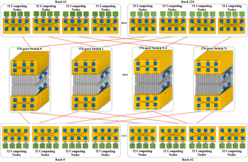
Figure S2: The architecture of Tianhe-2 supercomputer [2]. Tianhe-2 has 125 computing racks, each of which has 128 computing nodes. Therefore, Tianhe-2 has $16,000$ computing nodes in total, which are connected to switches following a customized fat-tree topology.

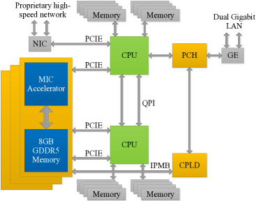
Figure S3: The architecture of a computing node in Tianhe-2 supercomputer [2]. Each node comprises 2 CPUs and 3 MIC accelerators.

To obtain the capacity bound of computing permanents classically, we tried exploiting as many computing resources of Tianhe-2 as possible. We parallelized and optimized the programs of Ryser’s algorithm and BB/FG’s algorithm on Tianhe-2 supercomputer [2]. The architecture of Tianhe-2 is shown in FIG. S2 and FIG. S3. The performance parameters of Tianhe-2 is listed in TABLE SVI. Before the large-scale test, we use a subsystem of Tianhe-2 with no more than 256 computing nodes to optimize and evaluate our programs. Ryser’s algorithm was tested with only CPUs, while BB/FG’s algorithm was tested in two types of configurations: running with only CPUs, or hybrid running with both CPUs and the co-processors denoted as MIC. Note that this 256-node subsystem still has a theoretical peak performance of 848.4 Teraflops that may be ranked in top 160 in the Top500 list in Nov. 2015.

The key of gaining performance improvement from a parallel computer system is to implement the parallelism of the program and guarantee its good scalability when using massive computing resources. Both Ryser’s and BB/FG’s algorithms could be easily implemented with effective parallelism. Though the two algorithms being executed in Gray code order decreases the time complexity by a factor $n$ compared with the original time complexity of $O(n^{2}\cdot 2^{n})$, this leads to so serious data dependency and memory cost that little parallelism could be implemented. Thus the algorithms with original execution order is chosen for supercomputer platform.

I.1 Utilizing Multiple CPUs (and CPU cores)

We used MPI library to generate multiple processes, exploiting the parallelism between CPUs, and OpenMP to produce multiple threads, exploiting that between CPU cores. As shown in Algorithm 1 and Algorithm 2, different processes have no data dependency except the data broadcast and the final reduce operation (line 6, 8 and 17 of Algorithm 1 and Algorithm 2) in which the main process (process 0) gathers data from other processes. This brings the good scalability of the parallel programs.

Algorithm 1 Parallelized Ryser’s algorithm

1:$A$: an $n\times n$ matrix; $P$: number of processes

2:$Per$: Permanent of A

3:Initialization;$\triangleright$ For parallelization using MPI

4:Set $rank$ to current process ID;

5:if $rank==0$ then

6:     Generate matrix and broadcast data;

7:else

8:     Receive data from process 0;

9:end if

10:$length=\lceil(2^{n}-1)/P\rceil$;

11:$start=rank*length$;

12:$end=\min(start+length,2^{n}-1)$;

13:for $iter=start$ to $end$ do$\triangleright$ Parallelized using OpenMP

14:     Generate set $S$ ($i\in S$ iff $i^{\text{th}}$ bit of $iter$ is 1);

15:     $Per=Per+(-1)^{|S|}\prod_{i=1}^{n}\sum_{j\in S}a_{ij}$;

16:end for

17:Sum $Per$s from all processes & store result on process 0;

18:if $n$ is odd and $rank==0$ then

19:     $Per=-1*Per$;

20:end if

21:Process 0 outputs $Per$;

Algorithm 2 Parallelized BB/FG’s algorithm

1:$A$: an $n\times n$ matrix; $P$: number of processes

2:$Per$: Permanent of A

3:Initialization;$\triangleright$ For parallelization using MPI

4:Set $rank$ to current process ID;

5:if $rank==0$ then

6:     Generate matrix and broadcast data;

7:else

8:     Receive data from the process 0;

9:end if

10:$length=\lceil(2^{n-1}-1)/P\rceil$;

11:$start=rank*length$;

12:$end=\min(start+length,2^{n-1}-1)$;

13:for $iter=start$ to $end$ do$\triangleright$ Parallelized using OpenMP

14:     Generate set $\delta=\{\delta_{i}\}$ ($\delta_{i}=1$ if the $i^{\text{th}}$ bit of $iter$ is 1, $\delta_{i}=-1$ otherwise);

15:     $Per=Per+(\prod_{k=1}^{n}\delta_{k})\prod_{j=1}^{n}\sum_{i=1}^{n}\delta_{i}a_{ij}$;

16:end for

17:Sum $Per$s from all processes & store result on process 0;

18:if $rank==0$ then

19:     $Per=Per/2^{n-1}$;

20:end if

21:Process 0 outputs $Per$;

I.2 Load Balance

We optimized the parallelized Ryser’s algorithm through load balance. In Algorithm 1, within the calculation of $\sum_{j\in S}a_{ij}$, the number of add operations is related to $|S|$. However, different $S$s generated from $iter$ in Algorithm 1 may have different sizes, leading to an imbalance loads. Therefore, we designed an optimizing algorithm with load balance, as Algorithm 3 shows. However, BB/FG’s algorithm is free from the imbalance problem because each iteration in the loop of Algorithm 2 always performs $n$ add/subtract operations.

Algorithm 3 Ryser’s algorithm with load balance

1:$A$: an $n\times n$ matrix; $P$: number of processes

2:$Per$: Permanent of A

3:Initialization;$\triangleright$ For parallelization using MPI

4:Set $rank$ to current process ID;

5:if $rank==0$ then

6:     Generate matrix and broadcast data;

7:else

8:     Receive data from the process 0;

9:end if

10:$length=\lceil(2^{n-1}-1)/P\rceil$;

11:$start=rank*length$;

12:$end=\min(start+end,2^{n-1}-1)$;

13:for $iter=start$ to $end$ do$\triangleright$ Parallelized using OpenMP

14:     Generate set $S$ ($i\in S$ iff $i^{\text{th}}$ bit of $iter$ is 1);

15:     $Per=Per+(-1)^{|S|}\prod_{i=1}^{n}\sum_{j\in S}a_{ij}$;

16:     Generate the complementary set $S_{C}$ of $S$;

17:     $Per=Per+(-1)^{|S_{C}|}\prod_{i=1}^{n}\sum_{j\in S_{C}}a_{ij}$;

18:end for

19:Sum $Per$s from all processes & store result on process 0;

20:if $n$ is odd and $rank==0$ then

21:     $Per=-1*Per$;

22:end if

23:Process 0 outputs $Per$;

Algorithm 4 Vectorized BB/FG’s algorithm on MIC

1:$A$: an $n\times n$ matrix

2:$Per$: Permanent of A

3:Set $vsize$ to the length of a vector register;

4:for $iter=0$ to $2^{n-1}-1$ do

5:     Generate set $\delta=\{\delta_{i}\}$ ($\delta_{i}=1$ if the $i^{\text{th}}$ bit of $iter$ is 1, $\delta_{i}=-1$ otherwise);

6:     Set vector $(a_{ij})_{V}$ to $\left(a_{i,(j-1)\cdot vsize+1},\ldots a_{i,j\cdot vsize}\right)$;

7:     $(vt)_{V}=\prod_{j=1}^{n/vsize}\sum_{i=1}^{n}\delta_{i}(a_{ij})_{V}$;$\triangleright$ Vector operations

8:     Multiplicative reduction on vector $(vt)_{V}$ & store result on number $t$;

9:     $Per=Per+(\prod_{k=1}^{n}\delta_{k})\cdot t$;

10:end for

11:$Per=Per/2^{n-1}$;

12:Output $Per$;

Algorithm 5 Heterogeneous BB/FG’s algorithm

1:$A$: an $n\times n$ matrix; $P$: number of processes

2:$Per$: Permanent of A

3:Initialization;$\triangleright$ For parallelization using MPI

4:Dispatch computing tasks between CPUs and MICs;

5:Sum $Per$s from MICs & store result on host;

6:Sum $Per$s from all processes & store result on process 0;

7:Process 0 computes $Per=Per/2^{n-1}$ & outputs $Per$;

I.3 Utilizing both CPUs and MICs

To make full use of computing power of Tianhe-2, we implemented a vectorized BB/FG’s algorithm for utilizing MIC accelerators. After several optimization steps, shown in TABLE SI, the final BB/FG’s algorithm is Algorithm 4. Finally, we combined all optimization techniques and implemented a heterogeneous algorithm, Algorithm 5, for utilizing all CPUs and accelerators of Tianhe-2.

Table SI: History of optimizations for co-processors. Some attempts that are not efficient are not listed, such as using mask operation for completing $\delta$ related computation.

Program Version	Optimization steps	Speedup
1	Naive implementation	$1\times$
2	Vectorization of matrix operation ($\sum_{i=1}^{N}\delta_{i}a_{ij}$)	$\sim$$1.6\times$
3	Vectorization of multiplicative reduction	$\sim$$1.8\times$
4	Multi-thread optimization	$\sim$$100\times$
5	Multi-MIC optimization	$\sim$$300\times$
6	Heterogeneous optimization with CPUs & MICs	$\sim$$370\times$
7	Optimized the vectorization scheme	$\sim$$500\times$

I.4 Efficiency

Figure S1: Efficiency for utilizing co-processors. The theoretical peak performance of a co-processor, Intel Xeon Phi, is 1.003 Teraflops. The performance of programs with only vectorized arithmetic instructions shows the capacity bound of the co-processor in real tests regardless of applications. The performance of two tailored programs takes the features of applications into consideration.

The optimized program for co-processors has a performance of 77.4 Gigaflops, about 7.71% of the theoretical peak performance. To evaluate the efficiency in more details, we tested several programs to put the co-processors into real tests.

As shown in FIG. S1, a program with only vectorized fused multiply-add instructions has a performance of 97.37% of the theoretical peak performance, while that with only add/subtract/multiply instructions has an efficiency of 48.55%.

The tests with only vectorized arithmetic instructions do not take the features of applications into consideration. To evaluate how efficiently we have been utilizing CPUs and co-processors for BB/FG’s algorithm, we tailored the program by removing implementation-related instructions as many as possible. The tailored programs, in TABLE SII, are viewed as the baselines. We compared several implementations for $\delta$-related calculation in Equation (S2) and adopted that, using branch instructions, with the highest efficiency in the final program. The program labelled “complete” in TABLE SII contains these branch instructions, while the program labelled “partial” doesn’t. If we take the tailored program with complete arithmetic operations left as a baseline, the average efficiencies are 97.0% and 86.0% for CPUs and co-processors respectively. If we take the program with partial arithmetic operations left, the average efficiencies are 74.0% and 26.3%.

Table SII: Programs for efficiency evaluation. “Normal” denotes the normal program. “Complete” denotes the tailored program labelled “program consisting of complete arithmetic operations” in FIG. 3, and “partial” denotes that labelled “program consisting of partial arithmetic operations” in FIG. 3. The programs for co-processors are vectorized. Only loop parts of the programs, line 13-16 in Algorithm 2 and line 4-10 in Algorithm 4, are discussed here.

Program	Instructions contained	Related equations
Normal	(vectorized) add/subtract instructions	$\sum_{\delta}\left(\prod_{k=1}^{n}\delta_{k}\right)\prod_{i=1}^{n}\sum_{j=1}^{n}\delta_{j}a_{ij}$
	(vectorized) multiply instructions
	branch instructions
	(vectorized) load/store instructions
Complete	(vectorized) add/subtract instructions	$\sum_{\delta}\left(\prod_{k=1}^{n}\delta_{k}\right)\prod_{i=1}^{n}\sum_{j=1}^{n}\delta_{j}a_{ij}$
	(vectorized) multiply instructions
	branch instructions
Partial	(vectorized) add/subtract instructions	$\sum_{\delta}\prod_{i=1}^{n}\sum_{j=1}^{n}a_{ij}$
	(vectorized) multiply instructions

I.5 Fitting

The fitting results can be found in TABLE SIII and TABLE SIV for Ryser’s algorithm and BB/FG’s algorithm respectively.

Table SIII: Fitting Result for Ryser’s algorithm. This table shows the fitting result for Ryser’s algorithm in FIG. 2(C).

Result:
Coefficients	Value	95% confidence bounds
		lower bound	upper bound
a:	$5.319\times 10^{-11}$	$4.135\times 10^{-11}$	$6.502\times 10^{-11}$
b:	$0.9924$	$0.9670$	$1.0170$
Goodness of fitting:
SSE:	29120	The smaller, the better
R_square:	0.9996	The closer to 1, the better
Adjusted R_square:	0.9996
RMSE:	39.15	The smaller, the better

Table SIV: Fitting Result for BB/FG’s algorithm. This table shows the fitting result for BB/FG’s algorithm in FIG. 2(D).

Result:
Coefficients	Value	95% confidence bounds
		lower bound	upper bound
a:	$9.805\times 10^{-12}$	$9.245\times 10^{-12}$	$1.037\times 10^{-11}$
b:	$0.87782$	$0.8916$	$0.8649$
Goodness of fitting:
SSE:	284.2	The smaller, the better
R_square:	0.994	The closer to 1, the better
Adjusted R_square:	0.9938
RMSE:	2.665	The smaller, the better

I.6 Architecture Transition

Co-processors provide strong processing power for state-of-the-art supercomputers. The co-processors, Intel Xeon Phi 31S1P, in Tianhe-2 were released in 2013. In this section, we compare it with some new co-processors as shown in TABLE SV.

For our program, there are three main aspects that may affect the performance obtained from co-processors. The first one is memory access performance due to the memory wall problem. Latency and bandwidth are two metrics associated with it. As shown in FIG. S1, the tailored program with complete arithmetic operations, from which memory access instructions have been removed, has a small speedup, $\sim$1.16$\times$. Meanwhile, the profiling shows that a memory bandwidth of only $\sim$0.3 GB/s is requested by our program. These indicate that our program is compute intensive and its performance is mainly dominated by the computing part. The second aspect is multi-thread optimization for a single core. In Intel Xeon Phi 31S1P, each core has four threads. The tests show that multi-thread optimization can utilize the vector processing unit in each core with as high efficiency as possible. The last one is multi-thread optimization for multiple cores. Our program has only one inter-thread communication in the final phase of each thread, which is a reduction operation shown in line 9 of Algorithm 4. This brings the good scalability of multi-thread optimizations.

The Knights Landing microarchitecture integrates on-package memory for significantly higher memory bandwidth. For example, Intel Xeon Phi 7290 has a MCDRAM (Multi-Channel DRAM) bandwidth of $400+$ GB/s. Besides, the peak double precision performance of single core and whole co-processor are both upgraded. Even though memory bandwidth is not the bottleneck of our program, we still could expect optimistically a speedup of $\sim$$3\times$ on Intel Xeon Phi 7290 because of the advance of the peak performance.

NVIDIA Volta GV100 has much more performance than other co-processors. However, it adopts Volta, an NVIDIA-developed GPU microarchitecture. Compared to Intel Xeon Phi 31S1P, it has different microarchitecture and different programming model. Thus, it is hard to compare the performance of our program on NVIDIA Volta GV100 with that on Intel Xeon Phi 31S1P. Considering the feature of the algorithm, we could expect a good performance optimistically. Matrix-2000 is a 128-core co-processor. Each core has two 256-bit vector processing units. Just like the analysis for NVIDIA Volta GV100, we believe it is not hard to exploit both thread-parallelism and SIMD-parallelism of Matrix-2000. In conclusion, our program is compute intensive along with good scalability, and we could expect the transplant of our program to other architectures has a good performance.

Table SV: Parameters of several latest co-processors. Intel Xeon Phi 31S1P released in 2013 is the co-processor of Tianhe-2. Intel Xeon Phi 7290, using MIC architecture, is released in 2016. NVIDIA Volta GV100 released in 2018 is used in several new supercomputers. Matrix-2000 released in 2017 is used in Tianhe-2A, an upgraded system.

Co-processor	Intel Xeon Phi 31S1P	Intel Xeon Phi 7290	NVIDIA Volta GV100	NUDT Matrix-2000
Microarchitecture	Knights Corner	Knights Landing	Volta	Matrix-2000
Release year	2013	2016	2018	2017
# of cores	57	72	CUDA: 5120 & Tensor: 640	128
# of threads	228	288	-	128
Clock (GHz)	1.1	1.5 (Turbo: 1.7)	1.132 (Boost: 1.628)	1.2
Memory bandwidth (GB/s)	320	102.4	870	143.1
MCDRAM bandwidth (GB/s)	-	400+	-	-
Peak DP compute (Teraflops)	1.003	3.456	7.400	2.458

II Analysis of the Precision Issue

The precision issue comes from the accumulated rounding errors introduced by limited word length of classical computers. Intermediate and final results are stored in double-precision floating-point format of IEEE-754 standard, where the total precision is decided by the 52-bit significand and an implicit bit. These 53 bits are approximately 16 decimal digits. Ryser’s algorithm may produce intermediate result that is extremely larger than the final result, so that the most important bits were used for the intermediate result, and the final result becomes as large as what could be truncated. For example, in the case when computing the permanent of a $30\times 30$ all-one matrix, the largest intermediate result is $30^{30}\approx 2.06\times 10^{44}$ while the final result is $30!\approx 2.65\times 10^{32}$ that is $10^{-12}$ smaller than the intermediate result. In these cases the errors of Ryser’s algorithm may not be omitted. For BB/FG’s algorithm, the final division guarantees the final result is in the same order of the intermediate data. Thus the error of BB/FG’s algorithm accumulates much slower, so that the results from BB/FG’s algorithm is much trustable than that produced by Ryser’s.

To evaluate errors of the two algorithms, we computed absolute errors and relative error rates of permanents of all-one matrices with different $n$. As shown in FIG. 5 and the detailed test data in TABLE SIX $\sim$ TABLE SXII, both the errors of Ryser’s algorithm and BB/FG’s algorithm grow exponentially with the increase of $n$ according to the fitting lines. However, the relative error rates of Ryser’s algorithm reaches nealy 100% when $n\geq 30$, and the errors of Ryser’s algorithm are approximately $10^{7}\sim 10^{9}$ larger than that of BB/FG’s algorithm, while the the fit-line predicts the relative error rate of BB/FG’s algorithm for a $50\times 50$ all-one matrix was about $0.0006\%$, and error rates does not exceed $10\%$ when the order of matrix is below 60. These results indicate that for relatively large $n$, the precision issue overburdens Ryser’s algorithm and BB/FG’s algorithm could still maintain the accuracy. Our results recommend BB/FG’s algorithm for the classical rival of quantum Boson sampling in the future research when the experiment scales up to a certain size, rather than Ryser’s algorithm that most considered before.

Realistically, the randomness of the built matrices make their permanents hard to evaluate. To confirm the precision issue in more realistic situations, we generated three types of random matrices, as shown in FIG. 5, and compare the results of the two algorithms. The errors of random unitary matrices and randomly derived matrices were marginal, thus we believe these results are trustable. But that of specially derived matrix chosen were still very large. The growing speed of errors of specially derived matrices is exponential. This suggests a double check with both two algorithms may be necessary for future research to verify results produced by classical computers. Besides, the precision issue implicates quantum computation may outperforms classical computation not just in speed, but also in precision sometimes.

III Detailed Test Data

III.1 Speed Performance

TABLE SVII and TABLE SVIII show the detailed test data of Ryser’s algorithm and BB/FG’s algorithm respectively. Some of data in these tables is used in FIG. 2 (main text).

Some screenshots and a photograph are shown here. FIG. S4 and FIG. S5 are screenshots in which Tianhe-2 was computing the permanent of a $45\times 45$ matrix. FIG. S6 shows an case of error in which some node failed during the execution.

III.2 Precision Performance

TABLE SIX $\sim$ TABLE SXII show the detailed test errors of BB/FG’s algorithm and Ryser’s algorithm. TABLE SIX and TABLE SXI show results for real matrices, and some of data is used in FIG. 5 (main text). TABLE SX and TABLE SXII show results for complex matrices.

Performing add operations in different orders may produce different intermediate results, which may bring different accumulated rounding errors. We tested Ryser’s algorithm with different orders of add operations. As shown in TABLE SXIII, we found the precision issue of Ryser’s algorithm became worse in some cases.

TABLE SXIV, TABLE SXV and TABLE SXVI show the detailed test errors for random matrices, and some of data is used in FIG. 5 (main text).

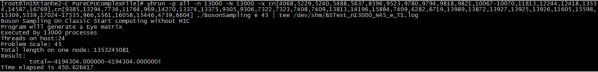
Figure S4: Screenshot of computing the permanent of a $45\times 45$ matrix on 13,000 nodes. The command line is “yhrun -p all -n 13000 -N 13000 -x cn[4068…6604] ./BosonSampling e 45 $|$ tee /dev/shm/BSTest_n13000_N45_e_T1.log”, where “yhrun” is the command to submit the task, “-p all” means the program would be executed on all the partitions of Tianhe-2, “-n 13000 -N 13000” means we would start 13,000 processes on 13,000 computing nodes, “-x cn[4068…6604]” defines the nodes that we won’t use for this computation and “./BosonSampling e 45” shows the input is a $45\times 45$-matrix with diagonal elements to be $1+i$ and other elements to be 0. The output would be recorded in file “/dev/shm/BSTest_n13000_N45_e_T1.log”. The line after “Result:” gives the computing result, which equals to the theoretical value $(1+i)^{45}$, and the last line gives the execution time in unit of seconds.

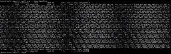
Figure S5: Screenshot of the node list of the 13,000 nodes used. The command line is “yhq -n BosonSampling”, which output the job with the executive named “BosonSampling” in the job sequence, the partition where this job was allocated and above all, and the node list of this job.

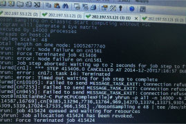
Figure S6: Photograph that shows error occurred during the computation on 14,000 nodes. Errors occurred more frequently when the number of nodes increases [3]. In this photograph, the node cn1561 failed during the execution, leading to the job termination and more errors in the node communication.

Table SVI: Performance Parameters of Tianhe-2 Supercomputer.

Item		Parameters of a node	Parameters of the System
Peak Performance		3.43 Teraflops	54.90 Petaflops
Processor	Intel Xeon E5 (12 cores)	2 (24 cores)	32,000 (384 thousand cores)
	Xeon Phi (57 cores)	3 (171cores)	48,000 (2.736 million Cores)
Memory Storage Capacity		64GB+8GB (Xeon Phi)	1.408PB
Disk Capacity		12.4PB
Mainboard (Two computing nodes)		8,000
Front-Ending Processor FT-1500(16 cores)		4,096
Interconnect Network		TH Express-2
Operating System		Kylin
Power Consumption		24 MW (17.808 MW without cooling system)

Table SVII: Execution time of Ryser’s algorithm (with only CPUs). The data of “Ryser@CPU” in FIG. 2 comes from this table. We used $P$ computing nodes to compute permanents of $n\times n$ matrices.

$P$	$n$	Execution time (s)	$P$	$n$	Execution time (s)	$P$	$n$	Execution time (s)
1	25	1.9642$\pm$0.2372	2	26	2.1562$\pm$0.2068	4	27	2.3908$\pm$0.1985
1	26	3.7839$\pm$0.2816	2	27	4.293$\pm$0.4017	4	28	4.7673$\pm$0.3210
1	27	7.6726$\pm$0.5345	2	28	8.6394$\pm$0.4483	4	29	9.3054$\pm$0.5000
1	28	15.9046$\pm$1.1006	2	29	17.6308$\pm$1.5244	4	30	18.8293$\pm$1.1771
1	29	31.8353$\pm$1.5959	2	30	34.267$\pm$2.0059	4	31	37.5951$\pm$2.0244
1	30	68.1029$\pm$3.5834	2	31	71.9743$\pm$1.2699	4	32	75.6077$\pm$0.8866
1	31	143.1606$\pm$3.0337	2	32	148.82$\pm$0.4387	4	33	159.1373$\pm$3.7312
8	28	2.7479$\pm$0.1168	16	29	2.8932$\pm$0.1206	32	30	3.2313$\pm$0.0400
8	29	5.3319$\pm$0.4006	16	30	5.7524$\pm$0.2777	32	31	6.4901$\pm$0.1221
8	30	9.803$\pm$0.3052	16	31	11.7995$\pm$1.0153	32	32	12.5818$\pm$1.0329
8	31	20.4626$\pm$0.8248	16	32	22.9742$\pm$1.7605	32	33	23.8788$\pm$1.6136
8	32	39.3735$\pm$1.5259	16	33	43.5551$\pm$1.7533	32	34	47.7301$\pm$1.3930
8	33	79.6846$\pm$1.0417	16	34	87.3021$\pm$5.3410	32	35	93.319$\pm$6.8016
8	34	165.1047$\pm$1.9254	16	35	176.1717$\pm$2.0559	32	36	186.7612$\pm$5.0536
64	31	3.4116$\pm$0.0873	128	32	3.5867$\pm$0.0201	256	33	3.9325$\pm$0.2320
64	32	6.708$\pm$0.2296	128	33	7.0565$\pm$0.1693	256	34	7.8038$\pm$0.5269
64	33	13.8701$\pm$1.8249	128	34	16.0373$\pm$2.2439	256	35	16.0211$\pm$1.0699
64	34	25.9721$\pm$1.7686	128	35	28.4909$\pm$1.8840	256	36	30.9905$\pm$1.4728
64	35	51.6904$\pm$5.1145	128	36	54.5887$\pm$6.6629	256	37	59.1407$\pm$4.2963
64	36	98.3382$\pm$1.9439	128	37	103.0265$\pm$5.2002	256	38	108.5136$\pm$3.4498
64	37	190.9616$\pm$4.0806	128	38	203.6487$\pm$9.3798	256	39	210.7175$\pm$12.3217

Table SVIII: Execution time of heterogeneous BB/FG’s algorithm (with both CPUs and MICs). The data of “BB/FG@Hybrid” in FIG. 2 and the fitting data in FIG. 2(C) come from this table. We used $P$ computing nodes to compute permanents of $n\times n$ matrices.

$P$	$n$	Execution time (s)	$P$	$n$	Execution time (s)	$P$	$n$	Execution time (s)
1	24	1.2384	2	25	1.0713	4	26	1.4582
1	25	1.0907	2	26	1.1171	4	27	1.5171
1	26	1.3009	2	27	1.4052	4	28	1.8441
1	27	1.6853	2	28	1.8302	4	29	2.3602
1	28	2.5140	2	29	2.8678	4	30	3.6961
1	29	4.3374	2	30	4.6822	4	31	6.1990
1	30	8.0175	2	31	9.0503	4	32	10.744
1	31	15.130	2	32	15.828	4	33	25.512
8	27	1.4967	16	28	1.5002	32	29	1.3799
8	28	1.6205	16	29	1.6593	32	30	1.6045
8	29	1.9648	16	30	1.9986	32	31	1.9624
8	30	2.6284	16	31	2.7252	32	32	2.7685
8	31	4.0077	16	32	4.1378	32	33	5.4228
8	32	6.4726	16	33	8.7461	32	34	9.9724
8	33	15.832	16	34	16.907	32	35	19.550
8	34	31.572	16	35	32.646	32	36	39.477
8	35	60.678	16	36	65.492	32	37	80.358
64	30	1.3939	128	31	1.4278	256	32	1.6232
64	31	1.5781	128	32	1.9457	256	33	1.9047
64	32	1.9385	128	33	2.1552	256	34	2.6021
64	33	3.3056	128	34	4.3292	256	35	4.5121
64	34	5.4466	128	35	5.9397	256	36	8.2317
64	35	11.228	128	36	15.533	256	37	15.877
64	36	21.428	128	37	23.652	256	38	31.815
64	37	44.767	128	38	46.065	256	39	66.710
64	38	84.098	128	39	133.18	256	40	132.35

Table SIX: Errors of BB/FG’s algorithm for real matrices. Some data in FIG. 5 comes from this table. We did the precision test by computing the permanent of an $n\times n$ all-$r$ real matrix, in which each element has a real value of $r$. In this case, the permanent in theory is $r^{n}\cdot n!$. In the table, $AbsErr=\left|Per_{\text{BB/FG}}-Per_{\text{Theory}}\right|$ and $RelErr=\left|(Per_{\text{BB/FG}}-Per_{\text{Theory}})/Per_{\text{Theory}}\right|$.

$n$	$r$	$Per_{\text{BB/FG}}$	$Per_{\text{Theory}}$	$AbsErr$	$RelErr$	$r$	$Per_{\text{BB/FG}}$	$Per_{\text{Theory}}$	$AbsErr$	$RelErr$
17	1	3.56E+14	3.56E+14	2.00E+00	5.62E-15	0.1	3.56E-03	3.56E-03	3.64E-17	1.02E-14
18	1	6.40E+15	6.40E+15	1.20E+02	1.87E-14	0.1	6.40E-03	6.40E-03	2.78E-16	4.35E-14
19	1	1.22E+17	1.22E+17	9.92E+02	8.15E-15	0.1	1.22E-02	1.22E-02	1.18E-15	9.67E-14
20	1	2.43E+18	2.43E+18	2.00E+04	8.21E-15	0.1	2.43E-02	2.43E-02	4.25E-15	1.75E-13
21	1	5.11E+19	5.11E+19	2.74E+06	5.36E-14	0.1	5.11E-02	5.11E-02	4.36E-15	8.54E-14
22	1	1.12E+21	1.12E+21	1.02E+08	9.11E-14	0.1	1.12E-01	1.12E-01	6.60E-14	5.87E-13
23	1	2.59E+22	2.59E+22	1.20E+10	4.63E-13	0.1	2.59E-01	2.59E-01	1.06E-13	4.08E-13
24	1	6.20E+23	6.20E+23	3.27E+11	5.28E-13	0.1	6.20E-01	6.20E-01	7.66E-13	1.23E-12
25	1	1.55E+25	1.55E+25	8.28E+12	5.34E-13	0.1	1.55E+00	1.55E+00	4.33E-12	2.79E-12
26	1	4.03E+26	4.03E+26	1.94E+15	4.81E-12	0.1	4.03E+00	4.03E+00	7.01E-12	1.74E-12
27	1	1.09E+28	1.09E+28	1.47E+17	1.35E-11	0.1	1.09E+01	1.09E+01	8.24E-11	7.57E-12
28	1	3.05E+29	3.05E+29	4.95E+17	1.62E-12	0.1	3.05E+01	3.05E+01	2.18E-10	7.15E-12
29	1	8.84E+30	8.84E+30	1.45E+20	1.64E-11	0.1	8.84E+01	8.84E+01	2.76E-09	3.12E-11
30	1	2.65E+32	2.65E+32	3.42E+22	1.29E-10	0.1	2.65E+02	2.65E+02	4.66E-09	1.76E-11
31	1	8.22E+33	8.22E+33	1.37E+24	1.67E-10	0.1	8.22E+02	8.22E+02	5.54E-08	6.73E-11
32	1	2.63E+35	2.63E+35	1.28E+26	4.87E-10	0.1	2.63E+03	2.63E+03	9.49E-07	3.61E-10
33	1	8.68E+36	8.68E+36	3.95E+27	4.55E-10	0.1	8.68E+03	8.68E+03	3.12E-07	3.60E-11
34	1	2.95E+38	2.95E+38	4.64E+28	1.57E-10	0.1	2.95E+04	2.95E+04	1.25E-05	4.25E-10
35	1	1.03E+40	1.03E+40	6.32E+30	6.12E-10	0.1	1.03E+05	1.03E+05	1.32E-04	1.28E-09
36	1	3.72E+41	3.72E+41	2.13E+33	5.72E-09	0.1	3.72E+05	3.72E+05	1.70E-03	4.56E-09
17	10	3.56E+31	3.56E+31	6.98E+17	1.96E-14	0.2	466.2066	466.2066	3.98E-12	8.53E-15
18	10	6.40E+33	6.40E+33	1.11E+20	1.73E-14	0.2	1678.344	1678.344	6.62E-11	3.94E-14
19	10	1.22E+36	1.22E+36	2.01E+22	1.65E-14	0.2	6377.707	6377.707	6.37E-10	9.98E-14
20	10	2.43E+38	2.43E+38	4.99E+24	2.05E-14	0.2	25510.83	25510.83	4.34E-09	1.70E-13
21	10	5.11E+40	5.11E+40	1.86E+27	3.63E-14	0.2	107145.5	107145.5	6.05E-09	5.65E-14
22	10	1.12E+43	1.12E+43	4.23E+29	3.77E-14	0.2	471440.1	471440.1	2.95E-07	6.25E-13
23	10	2.59E+45	2.59E+45	3.28E+32	1.27E-13	0.2	2168624	2168624	7.00E-07	3.23E-13
24	10	6.20E+47	6.20E+47	7.70E+35	1.24E-12	0.2	10409397	10409397	1.49E-05	1.43E-12
25	10	1.55E+50	1.55E+50	3.87E+38	2.50E-12	0.2	52046984	52046984	2.18E-04	4.19E-12
26	10	4.03E+52	4.03E+52	4.48E+40	1.11E-12	0.2	2.71E+08	2.71E+08	1.96E-04	7.22E-13
27	10	1.09E+55	1.09E+55	7.44E+43	6.84E-12	0.2	1.46E+09	1.46E+09	1.09E-02	7.44E-12
28	10	3.05E+57	3.05E+57	4.22E+46	1.38E-11	0.2	8.18E+09	8.18E+09	1.11E-01	1.36E-11
29	10	8.84E+59	8.84E+59	1.07E+50	1.21E-10	0.2	4.75E+10	4.75E+10	8.67E-01	1.83E-11
30	10	2.65E+62	2.65E+62	1.67E+52	6.31E-11	0.2	2.85E+11	2.85E+11	2.53E+01	8.87E-11
31	10	8.22E+64	8.22E+64	1.27E+55	1.55E-10	0.2	1.77E+12	1.77E+12	9.90E+01	5.61E-11
32	10	2.63E+67	2.63E+67	1.31E+58	4.97E-10	0.2	1.13E+13	1.13E+13	6.26E+03	5.54E-10
33	10	8.68E+69	8.68E+69	5.22E+60	6.01E-10	0.2	7.46E+13	7.46E+13	2.02E+04	2.71E-10
34	10	2.95E+72	2.95E+72	1.25E+62	4.23E-11	0.2	5.07E+14	5.07E+14	2.64E+05	5.20E-10
35	10	1.03E+75	1.03E+75	5.46E+66	5.28E-09	0.2	3.55E+15	3.55E+15	1.03E+07	2.91E-09
36	10	3.72E+77	3.72E+77	5.22E+68	1.40E-09	0.2	2.56E+16	2.56E+16	1.25E+08	4.87E-09

Table SX: Errors of BB/FG’s algorithm for complex matrices. We did the precision test by computing the permanent of an $n\times n$ all-$r$ complex matrix, in which each element has a complex value of $r$. In this case, the permanent in theory is $r^{n}\cdot n!$. $\text{Real}(Per_{\text{BB/FG}})$ is the real part of $Per_{\text{BB/FG}}$, and $\text{Imag}(Per_{\text{BB/FG}})$ is the imaginary part. $AbsErr=\left|Per_{\text{BB/FG}}-Per_{\text{Theory}}\right|$ and $RelErr=\left|(Per_{\text{BB/FG}}-Per_{\text{Theory}})/Per_{\text{Theory}}\right|$.

$n$	$r$	$\text{Real}(Per_{\text{BB/FG}})$	$\text{Imag}(Per_{\text{BB/FG}})$	$\text{Real}(Per_{\text{Theory}})$	$\text{Imag}(Per_{\text{Theory}})$	$AbsErr$	$RelErr$
17	$1+i$	9.11E+16	9.11E+16	9.11E+16	9.11E+16	4.30E+02	3.34E-15
18	$1+i$	0.00E+00	3.28E+18	0.00E+00	3.28E+18	7.01E+04	2.14E-14
19	$1+i$	-6.23E+19	6.23E+19	-6.23E+19	6.23E+19	1.14E+06	1.29E-14
20	$1+i$	-2.49E+21	0.00E+00	-2.49E+21	0.00E+00	1.99E+07	8.00E-15
21	$1+i$	-5.23E+22	-5.23E+22	-5.23E+22	-5.23E+22	4.10E+09	5.55E-14
22	$1+i$	-1.57E+10	-2.30E+24	0.00E+00	-2.30E+24	2.11E+11	9.14E-14
23	$1+i$	5.29E+25	-5.29E+25	5.29E+25	-5.29E+25	3.45E+13	4.61E-13
24	$1+i$	2.54E+27	-3.49E+12	2.54E+27	0.00E+00	1.34E+15	5.27E-13
25	$1+i$	6.35E+28	6.35E+28	6.35E+28	6.35E+28	4.78E+16	5.32E-13
26	$1+i$	1.49E+17	3.30E+30	0.00E+00	3.30E+30	1.60E+19	4.84E-12
27	$1+i$	-8.92E+31	8.92E+31	-8.92E+31	8.92E+31	1.70E+21	1.35E-11
28	$1+i$	-5.00E+33	-5.16E+19	-5.00E+33	0.00E+00	8.10E+21	1.62E-12
29	$1+i$	-1.45E+35	-1.45E+35	-1.45E+35	-1.45E+35	3.37E+24	1.64E-11
30	$1+i$	-7.79E+23	-8.69E+36	0.00E+00	-8.69E+36	1.12E+27	1.29E-10
31	$1+i$	2.69E+38	-2.69E+38	2.69E+38	-2.69E+38	6.36E+28	1.67E-10
32	$1+i$	1.72E+40	0.00E+00	1.72E+40	0.00E+00	8.40E+30	4.87E-10
33	$1+i$	5.69E+41	5.69E+41	5.69E+41	5.69E+41	3.66E+32	4.55E-10
34	$1+i$	0.00E+00	3.87E+43	0.00E+00	3.87E+43	6.09E+33	1.57E-10
35	$1+i$	-1.35E+45	1.35E+45	-1.35E+45	1.35E+45	1.36E+40	7.12E-06
36	$1+i$	-9.75E+46	-1.13E+35	-9.75E+46	0.00E+00	5.58E+38	5.72E-09
17	$10+10i$	9.11E+33	9.11E+33	9.11E+33	9.11E+33	2.40E+20	1.86E-14
18	$10+10i$	0.00E+00	3.28E+36	0.00E+00	3.28E+36	6.02E+22	1.84E-14
19	$10+10i$	-6.23E+38	6.23E+38	-6.23E+38	6.23E+38	2.13E+25	2.41E-14
20	$10+10i$	-2.49E+41	-3.30E+26	-2.49E+41	0.00E+00	5.00E+27	2.01E-14
21	$10+10i$	-5.23E+43	-5.23E+43	-5.23E+43	-5.23E+43	2.69E+30	3.63E-14
22	$10+10i$	-3.05E+32	-2.30E+46	0.00E+00	-2.30E+46	1.43E+33	6.22E-14
23	$10+10i$	5.29E+48	-5.29E+48	5.29E+48	-5.29E+48	1.17E+36	1.57E-13
24	$10+10i$	2.54E+51	1.70E+38	2.54E+51	0.00E+00	2.91E+39	1.15E-12
25	$10+10i$	6.35E+53	6.35E+53	6.35E+53	6.35E+53	2.15E+42	2.40E-12
26	$10+10i$	6.58E+42	3.30E+56	0.00E+00	3.30E+56	3.67E+44	1.11E-12
27	$10+10i$	-8.92E+58	8.92E+58	-8.92E+58	8.92E+58	8.63E+47	6.84E-12
28	$10+10i$	-5.00E+61	1.32E+47	-5.00E+61	0.00E+00	6.91E+50	1.38E-11
29	$10+10i$	-1.45E+64	-1.45E+64	-1.45E+64	-1.45E+64	2.47E+54	1.21E-10
30	$10+10i$	1.37E+53	-8.69E+66	0.00E+00	-8.69E+66	5.48E+56	6.31E-11
31	$10+10i$	2.69E+69	-2.69E+69	2.69E+69	-2.69E+69	5.89E+59	1.55E-10
32	$10+10i$	1.72E+72	0.00E+00	1.72E+72	0.00E+00	8.57E+62	4.97E-10
33	$10+10i$	5.69E+74	5.69E+74	5.69E+74	5.69E+74	4.84E+65	6.01E-10
34	$10+10i$	-1.65E+65	3.87E+77	0.00E+00	3.87E+77	1.64E+67	4.23E-11
35	$10+10i$	-1.35E+80	1.35E+80	-1.35E+80	1.35E+80	1.36E+75	7.11E-06
36	$10+10i$	-9.75E+82	-2.95E+69	-9.75E+82	0.00E+00	1.37E+74	1.40E-09

Table SXI: Errors of Ryser’s algorithm for real matrices. Some data in FIG. 5 comes from this table. We did the precision test by computing the permanent of an $n\times n$ all-$r$ real matrix, in which each element has a real value of $r$. In this case, the permanent in theory is $r^{n}\cdot n!$. In the table, $AbsErr=\left|Per_{\text{Ryser}}-Per_{\text{Theory}}\right|$ and $RelErr=\left|(Per_{\text{Ryser}}-Per_{\text{Theory}})/Per_{\text{Theory}}\right|$.

$n$	$r$	$Per_{\text{Ryser}}$	$Per_{\text{Theory}}$	$AbsErr$	$RelErr$	$r$	$Per_{\text{Ryser}}$	$Per_{\text{Theory}}$	$AbsErr$	$RelErr$
17	1	3.56E+14	3.56E+14	3.08E+06	8.67E-09	0.1	3.56E-03	3.56E-03	1.26E-07	3.53E-05
18	1	6.40E+15	6.40E+15	7.86E+07	1.23E-08	0.1	6.40E-03	6.40E-03	3.74E-07	5.84E-05
19	1	1.22E+17	1.22E+17	8.14E+09	6.69E-08	0.1	1.22E-02	1.22E-02	4.90E-07	4.03E-05
20	1	2.43E+18	2.43E+18	3.80E+11	1.56E-07	0.1	2.43E-02	2.43E-02	2.01E-08	8.25E-07
21	1	5.11E+19	5.11E+19	2.94E+13	5.75E-07	0.1	5.11E-02	5.11E-02	5.78E-08	1.13E-06
22	1	1.12E+21	1.12E+21	2.08E+15	1.85E-06	0.1	1.12E-01	1.12E-01	1.93E-06	1.71E-05
23	1	2.59E+22	2.59E+22	5.99E+16	2.32E-06	0.1	2.59E-01	2.59E-01	1.22E-05	4.71E-05
24	1	6.20E+23	6.20E+23	1.15E+18	1.85E-06	0.1	6.20E-01	6.20E-01	4.60E-06	7.41E-06
25	1	1.55E+25	1.55E+25	2.27E+21	1.47E-04	0.1	1.55E+00	1.55E+00	7.27E-04	4.69E-04
26	1	4.03E+26	4.03E+26	4.62E+22	1.15E-04	0.1	4.03E+00	4.03E+00	5.97E-03	1.48E-03
27	1	1.09E+28	1.09E+28	2.51E+24	2.30E-04	0.1	1.11E+01	1.09E+01	1.75E-01	1.60E-02
28	1	3.05E+29	3.05E+29	3.26E+25	1.07E-04	0.1	2.93E+01	3.05E+01	1.14E+00	3.75E-02
29	1	8.67E+30	8.84E+30	1.73E+29	1.95E-02	0.1	7.57E+01	8.84E+01	1.27E+01	1.44E-01
30	1	2.85E+32	2.65E+32	1.94E+31	7.32E-02	0.1	6.15E+02	2.65E+02	3.50E+02	1.32E+00
31	1	7.58E+33	8.22E+33	6.39E+32	7.78E-02	0.1	-4.19E+03	8.22E+02	5.01E+03	6.09E+00
32	1	-2.49E+33	2.63E+35	2.66E+35	1.01E+00	0.1	6.65E+04	2.63E+03	6.39E+04	2.43E+01
33	1	8.35E+36	8.68E+36	3.31E+35	3.82E-02	0.1	-4.16E+05	8.68E+03	4.25E+05	4.89E+01
34	1	3.60E+38	2.95E+38	6.44E+37	2.18E-01	0.1	2.20E+06	2.95E+04	2.17E+06	7.34E+01
35	1	-5.42E+41	1.03E+40	5.52E+41	5.34E+01	0.1	-6.35E+06	1.03E+05	6.45E+06	6.25E+01
36	1	4.24E+43	3.72E+41	4.21E+43	1.13E+02	0.1	-3.05E+08	3.72E+05	3.06E+08	8.22E+02
17	10	3.56E+31	3.56E+31	8.65E+22	2.43E-09	0.2	4.66E+02	4.66E+02	2.75E-06	5.91E-09
18	10	6.40E+33	6.40E+33	1.95E+25	3.04E-09	0.2	1.68E+03	1.68E+03	1.29E-06	7.66E-10
19	10	1.22E+36	1.22E+36	4.69E+28	3.85E-08	0.2	6.38E+03	6.38E+03	2.64E-04	4.13E-08
20	10	2.43E+38	2.43E+38	7.63E+31	3.14E-07	0.2	2.55E+04	2.55E+04	8.12E-03	3.18E-07
21	10	5.11E+40	5.11E+40	3.07E+34	6.02E-07	0.2	1.07E+05	1.07E+05	4.65E-01	4.34E-06
22	10	1.12E+43	1.12E+43	2.19E+36	1.95E-07	0.2	4.71E+05	4.71E+05	8.81E+00	1.87E-05
23	10	2.59E+45	2.59E+45	2.73E+40	1.06E-05	0.2	2.17E+06	2.17E+06	1.06E+02	4.90E-05
24	10	6.20E+47	6.20E+47	3.83E+43	6.17E-05	0.2	1.04E+07	1.04E+07	8.29E+01	7.96E-06
25	10	1.55E+50	1.55E+50	8.36E+46	5.39E-04	0.2	5.21E+07	5.20E+07	2.44E+04	4.69E-04
26	10	4.03E+52	4.03E+52	6.24E+49	1.55E-03	0.2	2.70E+08	2.71E+08	4.00E+05	1.48E-03
27	10	1.10E+55	1.09E+55	8.37E+52	7.68E-03	0.2	1.48E+09	1.46E+09	2.34E+07	1.60E-02
28	10	2.95E+57	3.05E+57	9.56E+55	3.13E-02	0.2	7.88E+09	8.18E+09	3.07E+08	3.75E-02
29	10	9.49E+59	8.84E+59	6.46E+58	7.31E-02	0.2	4.06E+10	4.75E+10	6.84E+09	1.44E-01
30	10	1.92E+62	2.65E+62	7.31E+61	2.75E-01	0.2	6.61E+11	2.85E+11	3.76E+11	1.32E+00
31	10	1.07E+65	8.22E+64	2.50E+64	3.04E-01	0.2	-9.00E+12	1.77E+12	1.08E+13	6.09E+00
32	10	6.54E+66	2.63E+67	1.98E+67	7.51E-01	0.2	2.86E+14	1.13E+13	2.74E+14	2.43E+01
33	10	3.60E+70	8.68E+69	2.73E+70	3.14E+00	0.2	-3.58E+15	7.46E+13	3.65E+15	4.89E+01
34	10	-8.76E+73	2.95E+72	9.06E+73	3.07E+01	0.2	3.77E+16	5.07E+14	3.72E+16	7.34E+01
35	10	1.32E+77	1.03E+75	1.31E+77	1.27E+02	0.2	-2.18E+17	3.55E+15	2.22E+17	6.25E+01
36	10	-2.14E+80	3.72E+77	2.14E+80	5.75E+02	0.2	-2.10E+19	2.56E+16	2.10E+19	8.22E+02

Table SXII: Errors of Ryser’s algorithm for complex matrices. We did the precision test by computing the permanent of an $n\times n$ all-$r$ complex matrix, in which each element has a complex value of $r$. In this case, the permanent in theory is $r^{n}\cdot n!$. $\text{Real}(Per_{\text{Ryser}})$ is the real part of $Per_{\text{Ryser}}$, and $\text{Imag}(Per_{\text{Ryser}})$ is the imaginary part. $AbsErr=\left|Per_{\text{Ryser}}-Per_{\text{Theory}}\right|$ and $RelErr=\left|(Per_{\text{Ryser}}-Per_{\text{Theory}})/Per_{\text{Theory}}\right|$.

$n$	$r$	$\text{Real}(Per_{\text{Ryser}})$	$\text{Imag}(Per_{\text{Ryser}})$	$\text{Real}(Per_{\text{Theory}})$	$\text{Imag}(Per_{\text{Theory}})$	$AbsErr$	$RelErr$
17	$1+i$	9.11E+16	9.11E+16	9.11E+16	9.11E+16	1.12E+09	8.67E-09
18	$1+i$	0.00E+00	3.28E+18	0.00E+00	3.28E+18	4.03E+10	1.23E-08
19	$1+i$	-6.23E+19	6.23E+19	-6.23E+19	6.23E+19	5.89E+12	6.69E-08
20	$1+i$	-2.49E+21	0.00E+00	-2.49E+21	0.00E+00	3.89E+14	1.56E-07
21	$1+i$	-5.23E+22	-5.23E+22	-5.23E+22	-5.23E+22	4.25E+16	5.75E-07
22	$1+i$	-5.91E+17	-2.30E+24	0.00E+00	-2.30E+24	4.31E+18	1.87E-06
23	$1+i$	5.29E+25	-5.29E+25	5.29E+25	-5.29E+25	1.73E+20	2.32E-06
24	$1+i$	2.54E+27	-6.38E+21	2.54E+27	0.00E+00	7.92E+21	3.12E-06
25	$1+i$	6.35E+28	6.35E+28	6.35E+28	6.35E+28	1.33E+25	1.48E-04
26	$1+i$	1.44E+24	3.30E+30	0.00E+00	3.30E+30	6.83E+26	2.07E-04
27	$1+i$	-8.92E+31	8.92E+31	-8.92E+31	8.92E+31	2.90E+28	2.30E-04
28	$1+i$	-5.00E+33	2.40E+29	-5.00E+33	0.00E+00	5.85E+29	1.17E-04
29	$1+i$	-1.42E+35	-1.42E+35	-1.45E+35	-1.45E+35	4.00E+33	1.95E-02
30	$1+i$	3.91E+34	-9.33E+36	0.00E+00	-8.69E+36	6.37E+35	7.33E-02
31	$1+i$	2.48E+38	-2.48E+38	2.69E+38	-2.69E+38	2.96E+37	7.78E-02
32	$1+i$	-1.63E+38	0.00E+00	1.72E+40	0.00E+00	1.74E+40	1.01E+00
33	$1+i$	5.47E+41	5.47E+41	5.69E+41	5.69E+41	3.07E+40	3.82E-02
34	$1+i$	0.00E+00	4.71E+43	0.00E+00	3.87E+43	8.45E+42	2.18E-01
35	$1+i$	7.10E+46	-7.10E+46	-1.35E+45	1.35E+45	1.02E+47	5.34E+01
36	$1+i$	-1.11E+49	7.42E+47	-9.75E+46	0.00E+00	1.10E+49	1.13E+02
17	$10+10i$	9.11E+33	9.11E+33	9.11E+33	9.11E+33	3.13E+25	2.43E-09
18	$10+10i$	0.00E+00	3.28E+36	0.00E+00	3.28E+36	9.97E+27	3.04E-09
19	$10+10i$	-6.23E+38	6.23E+38	-6.23E+38	6.23E+38	3.39E+31	3.85E-08
20	$10+10i$	-2.49E+41	7.02E+33	-2.49E+41	0.00E+00	7.84E+34	3.15E-07
21	$10+10i$	-5.23E+43	-5.23E+43	-5.23E+43	-5.23E+43	3.98E+37	5.38E-07
22	$10+10i$	-2.36E+40	-2.30E+46	0.00E+00	-2.30E+46	2.72E+40	1.18E-06
23	$10+10i$	5.29E+48	-5.29E+48	5.29E+48	-5.29E+48	6.10E+43	8.15E-06
24	$10+10i$	2.54E+51	-4.61E+46	2.54E+51	0.00E+00	1.15E+47	4.54E-05
25	$10+10i$	6.36E+53	6.36E+53	6.35E+53	6.35E+53	4.44E+50	4.94E-04
26	$10+10i$	1.25E+52	3.30E+56	0.00E+00	3.30E+56	5.12E+53	1.55E-03
27	$10+10i$	-8.99E+58	8.99E+58	-8.92E+58	8.92E+58	9.69E+56	7.68E-03
28	$10+10i$	-4.84E+61	4.78E+58	-5.00E+61	0.00E+00	1.57E+60	3.14E-02
29	$10+10i$	-1.55E+64	-1.55E+64	-1.45E+64	-1.45E+64	1.50E+63	7.31E-02
30	$10+10i$	3.25E+64	-6.30E+66	0.00E+00	-8.69E+66	2.39E+66	2.76E-01
31	$10+10i$	3.51E+69	-3.51E+69	2.69E+69	-2.69E+69	1.16E+69	3.04E-01
32	$10+10i$	4.29E+71	0.00E+00	1.72E+72	0.00E+00	1.30E+72	7.51E-01
33	$10+10i$	2.36E+75	2.36E+75	5.69E+74	5.69E+74	2.53E+75	3.14E+00
34	$10+10i$	-5.63E+77	1.15E+79	0.00E+00	3.87E+77	1.11E+79	2.87E+01
35	$10+10i$	-1.73E+82	1.73E+82	-1.35E+80	1.35E+80	2.43E+82	1.27E+02
36	$10+10i$	5.60E+85	1.69E+82	-9.75E+82	0.00E+00	5.61E+85	5.75E+02

Table SXIII: Errors of Ryser’s algorithm from the order of add operations. We did the precision test by computing the permanent of an $n\times n$ all-one real matrix, the permanent of which is $n!$ in theory. We tested different orders of add operations on intermediate results from different iterations. For example, $\sigma_{0},\ldots\sigma_{7}$ represents eight intermediate results, $\prod_{i=1}^{n}\sum_{j\in S}a_{ij}$ in the iterations of Algorithm 1. Assume $\sigma_{0},\sigma_{2},\sigma_{4},\sigma_{8}$ correspond to the cases of $(-1)^{|S|}=1$ in Algorithm 1, and $\sigma_{1},\sigma_{3},\sigma_{5},\sigma_{7}$ correspond to that of $(-1)^{|S|}=-1$. “Original” performs $\sigma_{0}-\sigma_{1}+\sigma_{2}-\sigma_{3}+\sigma_{4}-\sigma_{5}+\sigma_{6}-\sigma_{7}$. “Random” performs add operations in a random order. “Merging” performs $(((\sigma_{0}-\sigma_{1})+(\sigma_{2}-\sigma_{3}))+((\sigma_{4}-\sigma_{5})+(\sigma_{6}-\sigma_{7})))$. “Separating” performs $(\sigma_{0}+\sigma_{2}+\sigma_{4}+\sigma_{6})-(\sigma_{1}+\sigma_{3}+\sigma_{5}+\sigma_{7})$.

$n$	$Per_{\text{Theory}}$	Original		Random		Merging		Separating
		$Per_{\text{Ryser}}$	$RelErr$	$Per_{\text{Ryser}}$	$RelErr$	$Per_{\text{Ryser}}$	$RelErr$	$Per_{\text{Ryser}}$	$RelErr$
8	4.03E+04	4.03E+04	0.00E+00	4.03E+04	0.00E+00	4.03E+04	0.00E+00	4.03E+04	0.00E+00
9	3.63E+05	3.63E+05	0.00E+00	3.63E+05	0.00E+00	3.63E+05	0.00E+00	3.63E+05	0.00E+00
10	3.63E+06	3.63E+06	0.00E+00	3.63E+06	0.00E+00	3.63E+06	0.00E+00	3.63E+06	0.00E+00
11	3.99E+07	3.99E+07	0.00E+00	3.99E+07	0.00E+00	3.99E+07	0.00E+00	3.99E+07	0.00E+00
12	4.79E+08	4.79E+08	0.00E+00	4.79E+08	0.00E+00	4.79E+08	0.00E+00	4.79E+08	0.00E+00
13	6.23E+09	6.23E+09	0.00E+00	6.23E+09	0.00E+00	6.23E+09	0.00E+00	6.23E+09	0.00E+00
14	8.72E+10	8.72E+10	0.00E+00	8.72E+10	1.32E-07	8.72E+10	0.00E+00	8.72E+10	9.18E-09
15	1.31E+12	1.31E+12	1.96E-10	1.31E+12	3.62E-07	1.31E+12	4.86E-10	1.31E+12	2.35E-08
16	2.09E+13	2.09E+13	8.81E-10	2.09E+13	1.29E-07	2.09E+13	9.57E-10	2.09E+13	1.36E-07
17	3.56E+14	3.56E+14	1.11E-08	3.56E+14	9.41E-05	3.56E+14	8.24E-09	3.56E+14	4.81E-07
18	6.40E+15	6.40E+15	7.73E-09	6.40E+15	1.46E-04	6.40E+15	2.59E-09	6.40E+15	2.57E-06
19	1.22E+17	1.22E+17	4.28E-08	1.22E+17	1.72E-04	1.22E+17	8.13E-08	1.22E+17	7.31E-05
20	2.43E+18	2.43E+18	2.60E-07	2.39E+18	1.64E-02	2.43E+18	2.46E-07	2.43E+18	4.51E-04
21	5.11E+19	5.11E+19	9.52E-07	3.64E+19	2.88E-01	5.11E+19	1.01E-06	5.11E+19	9.39E-04
22	1.12E+21	1.12E+21	2.88E-06	-3.60E+20	1.32E+00	1.12E+21	4.28E-06	1.14E+21	1.59E-02
23	2.59E+22	2.59E+22	4.15E-06	6.96E+23	2.59E+01	2.59E+22	1.39E-05	2.72E+22	5.02E-02
24	6.20E+23	6.20E+23	1.59E-05	-1.21E+25	2.04E+01	6.20E+23	2.18E-05	7.80E+23	2.57E-01
25	1.55E+25	1.55E+25	1.05E-04	-5.49E+27	3.55E+02	1.55E+25	1.28E-04	-3.50E+25	3.26E+00
26	4.03E+26	4.03E+26	1.53E-04	2.29E+30	5.67E+03	4.03E+26	4.36E-04	1.68E+28	4.07E+01
27	1.09E+28	1.09E+28	5.48E-04	-1.36E+32	1.25E+04	1.09E+28	1.35E-03	-2.95E+30	2.72E+02
28	3.05E+29	3.05E+29	1.83E-04	1.61E+34	5.27E+04	3.05E+29	1.12E-04	4.66E+32	1.53E+03
29	8.84E+30	8.54E+30	3.47E-02	-6.42E+36	7.26E+05	8.47E+30	4.16E-02	-1.08E+35	1.22E+04
30	2.65E+32	2.97E+32	1.18E-01	-7.86E+38	2.96E+06	2.98E+32	1.23E-01	3.13E+37	1.18E+05
31	8.22E+33	6.15E+33	2.53E-01	7.00E+41	8.52E+07	5.81E+33	2.94E-01	1.75E+38	2.12E+04
32	2.63E+35	8.21E+34	6.88E-01	-8.38E+43	3.19E+08	1.24E+35	5.29E-01	2.65E+41	1.01E+06

Table SXIV: Results comparing BB/FG’s algorithm and Ryser’s algorithm for $n\times n$ random unitary matrices. Some data of “Random unitary matrix” in FIG. 5 comes from this table. $\text{Real}(Per)$ is the real part of $Per$, and $\text{Imag}(Per)$ is the imaginary part. $RelErr=\left|(Per_{\text{Ryser}}-Per_{\text{BB/FG}})/Per_{\text{BB/FG}}\right|$. The tested matrices are generated by MATLAB.

$n$	$\text{Real}(Per_{\text{Ryser}})$	$\text{Imag}(Per_{\text{Ryser}})$	$\text{Real}(Per_{\text{BB/FG}})$	$\text{Imag}(Per_{\text{BB/FG}})$	$RelErr$
31	4.2230E-09	-1.9454E-09	4.2230E-09	-1.9454E-09	0
32	-4.1659E-09	-2.3246E-09	-4.1659E-09	-2.3246E-09	0
33	4.8134E-10	8.4106E-10	4.8134E-10	8.4106E-10	0
34	2.7587E-10	2.1718E-10	2.7587E-10	2.1718E-10	2.848E-07
35	-1.1053E-10	-7.2113E-10	-1.1053E-10	-7.2113E-10	1.371E-07
36	-5.5166E-11	-3.4459E-11	-5.5166E-11	-3.4459E-11	4.612E-07
37	-3.3585E-11	3.9724E-12	-3.3585E-11	3.9722E-12	5.039E-06
38	-5.6397E-11	-6.3709E-11	-5.6397E-11	-6.3709E-11	2.351E-07
39	-4.2777E-11	-1.2135E-11	-4.2777E-11	-1.2135E-11	4.498E-07
40	5.8951E-12	-2.1875E-11	5.8951E-12	-2.1875E-11	0

Table SXV: Results comparing BB/FG’s algorithm and Ryser’s algorithm for random-derived matrices. Some data of “Random-derived matrix” in FIG. 5 comes from this table. $\text{Real}(Per)$ is the real part of $Per$, and $\text{Imag}(Per)$ is the imaginary part. $RelErr=\left|(Per_{\text{Ryser}}-Per_{\text{BB/FG}})/Per_{\text{BB/FG}}\right|$. The tested matrices were derived from a $100\times 100$ unitary matrix.

$n$	$\text{Real}(Per_{\text{Ryser}})$	$\text{Imag}(Per_{\text{Ryser}})$	$\text{Real}(Per_{\text{BB/FG}})$	$\text{Imag}(Per_{\text{BB/FG}})$	$RelErr$
21	-4.3428E-12	-5.9702E-12	-4.3428E-12	-5.9702E-12	0
22	7.6833E-13	-3.9798E-13	7.6833E-13	-3.9798E-13	1.1557E-07
23	-3.7027E-12	1.6829E-12	-3.7027E-12	1.6829E-12	0
24	-3.4145E-12	1.6790E-12	-3.4145E-12	1.6790E-12	0
25	6.3631E-13	6.0936E-13	6.3631E-13	6.0936E-13	0
26	2.0950E-13	-3.6558E-13	2.0950E-13	-3.6558E-13	0
27	1.7856E-13	1.7049E-13	1.7856E-13	1.7049E-13	0
28	-1.4828E-14	-5.6576E-14	-1.4828E-14	-5.6576E-14	0
29	9.6421E-14	2.0312E-13	9.6421E-14	2.0312E-13	0
30	1.7654E-14	2.7364E-14	1.7654E-14	2.7364E-14	0
31	2.7628E-16	1.4029E-14	2.7628E-16	1.4029E-14	7.1269E-09
32	-1.7119E-14	1.3498E-14	-1.7119E-14	1.3498E-14	0
33	6.9880E-15	4.0715E-15	6.9880E-15	4.0715E-15	0
34	1.0924E-15	1.2235E-14	1.0924E-15	1.2235E-14	0
35	-1.0497E-16	-1.3781E-16	-1.0497E-16	-1.3781E-16	0
36	5.9267E-16	-1.9652E-16	5.9268E-16	-1.9652E-16	3.2030E-06
37	-3.5034E-16	-2.3051E-16	-3.5034E-16	-2.3051E-16	0
38	2.7198E-15	6.0656E-16	2.7198E-15	6.0656E-16	0
39	7.9334E-16	5.6975E-16	7.9334E-16	5.6975E-16	2.4763E-06
40	1.2277E-16	-2.4051E-16	1.2276E-16	-2.4051E-16	2.0768E-05
41	-1.2519E-16	1.7989E-16	-1.2519E-16	1.7989E-16	1.2905E-06
42	-5.1615E-16	-3.3737E-16	-5.1618E-16	-3.3742E-16	9.6984E-05
43	-8.8131E-17	3.3867E-16	-9.0932E-17	3.3741E-16	8.7707E-03
44	1.3425E-18	1.0379E-19	1.3424E-18	1.0375E-19	5.9686E-05

Table SXVI: Results comparing BB/FG’s algorithm and Ryser’s algorithm for special-derived matrices. Some data of “Special-derived matrix” in FIG. 5 comes from this table. $RelErr=\left|(Per_{\text{Ryser}}-Per_{\text{BB/FG}})/Per_{\text{BB/FG}}\right|$. The tested matrices were manually chosen from the $100\times 100$ real unitary matrix with elements all negative, and duplicated the rows and columns to enlarge the scale.

$n$	$Per_{\text{Ryser}}$	$Per_{\text{BB/FG}}$	$RelErr$
30	5.3072E-01	4.6606E-01	1.3874E-01
31	-2.2483E-01	-1.2863E-01	7.4793E-01
32	1.1668E+00	7.4303E-01	5.7034E-01
33	6.3670E+01	-3.6957E+00	1.8228E+01
34	3.5526E+01	2.1389E-01	1.6510E+02
35	1.4313E+04	-7.9309E+02	1.9047E+01
36	2.8634E+04	3.1883E+02	8.8812E+01
37	6.3388E+04	-7.0710E+01	8.9745E+02
38	1.3012E+07	2.5863E+03	5.0300E+03
39	-1.0717E+07	-4.8804E+03	2.1950E+03
40	-1.0307E+08	1.2365E+03	8.3360E+04

References

- [1] David Deutsch. Quantum theory, the church-turing principle and the universal quantum computer. Proceedings of the Royal Society of London A: Mathematical, Physical and Engineering Sciences, 400(1818):97–117, 1985.
- [2] Michael A. Nielsen and Isaac L. Chuang. Quantum Computation and Quantum Information: 10th Anniversary Edition. Cambridge University Press, New York, NY, USA, 10th edition, 2011.
- [3] Peter W. Shor. Algorithms for quantum computation: discrete logarithms and factoring. In Foundations of Computer Science, 1994 Proceedings., 35th Annual Symposium on, pages 124–134, Nov 1994.
- [4] Thorsten Kleinjung, Kazumaro Aoki, Jens Franke, Arjen K Lenstra, Emmanuel Thomé, Joppe W Bos, Pierrick Gaudry, Alexander Kruppa, Peter L Montgomery, Dag Arne Osvik, et al. Factorization of a 768-bit rsa modulus. In Annual Cryptology Conference, pages 333–350. Springer, 2010.
- [5] Austin G. Fowler, Matteo Mariantoni, John M. Martinis, and Andrew N. Cleland. Surface codes: Towards practical large-scale quantum computation. Phys. Rev. A, 86:032324, Sep 2012.
- [6] Enrique Martin-Lopez, Anthony Laing, Thomas Lawson, Roberto Alvarez, Xiao-Qi Zhou, and Jeremy L. O’Brien. Experimental realization of shor’s quantum factoring algorithm using qubit recycling. Nature Photonics, 6(11):773–776, 11 2012.
- [7] B. P. Lanyon, T. J. Weinhold, N. K. Langford, M. Barbieri, D. F. V. James, A. Gilchrist, and A. G. White. Experimental demonstration of a compiled version of shor’s algorithm with quantum entanglement. Phys. Rev. Lett., 99:250505, Dec 2007.
- [8] Alberto Politi, Jonathan C. F. Matthews, and Jeremy L. O’Brien. Shor’s quantum factoring algorithm on a photonic chip. Science, 325(5945):1221–1221, 2009.
- [9] S. Parker and M. B. Plenio. Efficient factorization with a single pure qubit and mixed qubits. Phys. Rev. Lett., 85:3049–3052, Oct 2000.
- [10] Chao-Yang Lu, Daniel E. Browne, Tao Yang, and Jian-Wei Pan. Demonstration of a compiled version of shor’s quantum factoring algorithm using photonic qubits. Phys. Rev. Lett., 99:250504, Dec 2007.
- [11] Thomas Monz, Daniel Nigg, Esteban A. Martinez, Matthias F. Brandl, Philipp Schindler, Richard Rines, Shannon X. Wang, Isaac L. Chuang, and Rainer Blatt. Realization of a scalable shor algorithm. Science, 351(6277):1068–1070, 2016.
- [12] Lieven MK Vandersypen, Matthias Steffen, Gregory Breyta, Costantino S Yannoni, Mark H Sherwood, and Isaac L Chuang. Experimental realization of shor’s quantum factoring algorithm using nuclear magnetic resonance. Nature, 414(6866):883–887, 2001.
- [13] Scott Aaronson and Alex Arkhipov. The computational complexity of linear optics. In Proceedings of the Forty-third Annual ACM Symposium on Theory of Computing, STOC ’11, pages 333–342, New York, NY, USA, 2011. ACM.
- [14] Stefan Scheel. Macroscopic Quantum Electrodynamics - Concepts and Applications. Acta Physica Slovaca, 58:675–809, Oct 2008.
- [15] Justin B. Spring, Benjamin J. Metcalf, Peter C. Humphreys, W. Steven Kolthammer, Xian-Min Jin, Marco Barbieri, Animesh Datta, Nicholas Thomas-Peter, Nathan K. Langford, Dmytro Kundys, James C. Gates, Brian J. Smith, Peter G. R. Smith, and Ian A. Walmsley. Boson sampling on a photonic chip. Science, 339(6121):798–801, 2013.
- [16] Matthew A. Broome, Alessandro Fedrizzi, Saleh Rahimi-Keshari, Justin Dove, Scott Aaronson, Timothy C. Ralph, and Andrew G. White. Photonic boson sampling in a tunable circuit. Science, 339(6121):794–798, 2013.
- [17] Max Tillmann, Borivoje Dakic, Rene Heilmann, Stefan Nolte, Alexander Szameit, and Philip Walther. Experimental boson sampling. Nature Photonics, 7(7):540–544, 07 2013.
- [18] Andrea Crespi, Roberto Osellame, Roberta Ramponi, Daniel J. Brod, Ernesto F. Galvao, Nicolo Spagnolo, Chiara Vitelli, Enrico Maiorino, Paolo Mataloni, and Fabio Sciarrino. Integrated multimode interferometers with arbitrary designs for photonic boson sampling. Nature Photonics, 7(7):545–549, 07 2013.
- [19] Scott Aaronson. Scattershot bosonsampling: A new approach to scalable bosonsampling experiments. http://www.scottaaronson.com/blog/?p=1579, 2013.
- [20] A. P. Lund, A. Laing, S. Rahimi-Keshari, T. Rudolph, J. L. O’Brien, and T. C. Ralph. Boson sampling from a gaussian state. Phys. Rev. Lett., 113:100502, Sep 2014.
- [21] Marco Bentivegna, Nicolò Spagnolo, Chiara Vitelli, Fulvio Flamini, Niko Viggianiello, Ludovico Latmiral, Paolo Mataloni, Daniel J. Brod, Ernesto F. Galvão, Andrea Crespi, Roberta Ramponi, Roberto Osellame, and Fabio Sciarrino. Experimental scattershot boson sampling. Science Advances, 1(3), 2015.
- [22] Keith R. Motes, Alexei Gilchrist, Jonathan P. Dowling, and Peter P. Rohde. Scalable boson sampling with time-bin encoding using a loop-based architecture. Phys. Rev. Lett., 113:120501, Sep 2014.
- [23] J. B. Spring, P. L. Mennea, B. J. Metcalf, P. C. Humphreys, J. C. Gates, H. L. Rogers, C. Soeller, B. J. Smith, W. S. Kolthammer, P. G. R. Smith, and I. A. Walmsley. A chip-based array of near-identical, pure, heralded single photon sources. ArXiv e-prints, 1603.06984, March 2016.
- [24] Jacques Carolan, Christopher Harrold, Chris Sparrow, Enrique Martín-López, Nicholas J. Russell, Joshua W. Silverstone, Peter J. Shadbolt, Nobuyuki Matsuda, Manabu Oguma, Mikitaka Itoh, Graham D. Marshall, Mark G. Thompson, Jonathan C. F. Matthews, Toshikazu Hashimoto, Jeremy L. O’Brien, and Anthony Laing. Universal linear optics. Science, 349(6249):711–716, 2015.
- [25] Hugo Defienne, Marco Barbieri, Ian A. Walmsley, Brian J. Smith, and Sylvain Gigan. Two-photon quantum walk in a multimode fiber. Science Advances, 2(1), 2016.
- [26] Peter P. Rohde and Timothy C. Ralph. Error tolerance of the boson-sampling model for linear optics quantum computing. Phys. Rev. A, 85:022332, Feb 2012.
- [27] Peter P. Rohde. Optical quantum computing with photons of arbitrarily low fidelity and purity. Phys. Rev. A, 86:052321, Nov 2012.
- [28] Saleh Rahimi-Keshari, Timothy C Ralph, and Carlton M Caves. Sufficient conditions for efficient classical simulation of quantum optics. Physical Review X, 6(2), 2016.
- [29] Keith R. Motes, Jonathan P. Dowling, and Peter P. Rohde. Spontaneous parametric down-conversion photon sources are scalable in the asymptotic limit for boson sampling. Phys. Rev. A, 88:063822, Dec 2013.
- [30] Keith R. Motes, Jonathan P. Dowling, Alexei Gilchrist, and Peter P. Rohde. Implementing bosonsampling with time-bin encoding: Analysis of loss, mode mismatch, and time jitter. Phys. Rev. A, 92:052319, Nov 2015.
- [31] Scott Aaronson and Alex Arkhipov. Bosonsampling is far from uniform. Quantum Info. Comput., 14(15-16):1383–1423, November 2014.
- [32] Nicolo Spagnolo, Chiara Vitelli, Marco Bentivegna, Daniel J. Brod, Andrea Crespi, Fulvio Flamini, Sandro Giacomini, Giorgio Milani, Roberta Ramponi, Paolo Mataloni, Roberto Osellame, Ernesto F. Galvao, and Fabio Sciarrino. Experimental validation of photonic boson sampling. Nature Photonics, 8(8):615–620, 08 2014.
- [33] S.-T. Wang and L.-M. Duan. Certification of Boson Sampling Devices with Coarse-Grained Measurements. ArXiv e-prints, 1601.02627, January 2016.
- [34] Peter P. Rohde, Keith R. Motes, Paul A. Knott, Joseph Fitzsimons, William J. Munro, and Jonathan P. Dowling. Evidence for the conjecture that sampling generalized cat states with linear optics is hard. Phys. Rev. A, 91:012342, Jan 2015.
- [35] Kaushik P. Seshadreesan, Jonathan P. Olson, Keith R. Motes, Peter P. Rohde, and Jonathan P. Dowling. Boson sampling with displaced single-photon fock states versus single-photon-added coherent states: The quantum-classical divide and computational-complexity transitions in linear optics. Phys. Rev. A, 91:022334, Feb 2015.
- [36] Jonathan P. Olson, Kaushik P. Seshadreesan, Keith R. Motes, Peter P. Rohde, and Jonathan P. Dowling. Sampling arbitrary photon-added or photon-subtracted squeezed states is in the same complexity class as boson sampling. Phys. Rev. A, 91:022317, Feb 2015.
- [37] Xiangke Liao, Liquan Xiao, Canqun Yang, and Yutong Lu. Milkyway-2 supercomputer: System and application. Frontiers of Computer Science in China, 8(3):345–356, June 2014.
- [38] Xuejun Yang, Zhiyuan Wang, Jingling Xue, and Yun Zhou. The reliability wall for exascale supercomputing. IEEE Transactions on Computers, 61(6):767–779, June 2012.

References

- [1] Jerrum, M, Sinclair, A, Vigoda, E. A polynomial-time approximation algorithm for the permanent of a matrix with nonnegative entries. Journal of the ACM, 2004, 51(4):671-97.
- [2] Liao, X, Xiao, L, Yang, C et al. Milkyway-2 supercomputer: System and application. Frontiers of Computer Science in China, 2014, 8(3):345-56.
- [3] Yang, X, Wang, Z, Xue, J et al. The reliability wall for exascale supercomputing. IEEE Transactions on Computers, 2012, 61(6):767-79.