Guaranteed bounds on the Kullback-Leibler divergence of univariate mixtures using piecewise log-sum-exp inequalities

Frank Nielsen Frank Nielsen is with École Polytechnique and Sony Computer Science Laboratories Inc. E-mail: Frank.Nielsen@acm.org    Ke Sun Ke Sun is with École Polytechnique, E-mail: sunk.edu@gmail.com.
Abstract

Information-theoretic measures such as the entropy, cross-entropy and the Kullback-Leibler divergence between two mixture models is a core primitive in many signal processing tasks. Since the Kullback-Leibler divergence of mixtures provably does not admit a closed-form formula, it is in practice either estimated using costly Monte-Carlo stochastic integration, approximated, or bounded using various techniques. We present a fast and generic method that builds algorithmically closed-form lower and upper bounds on the entropy, the cross-entropy and the Kullback-Leibler divergence of mixtures. We illustrate the versatile method by reporting on our experiments for approximating the Kullback-Leibler divergence between univariate exponential mixtures, Gaussian mixtures, Rayleigh mixtures, and Gamma mixtures.

1 Introduction

Mixture models are commonly used in signal processing. A typical scenario is to use mixture models [15, 30, 17] to smoothly model histograms. For example, Gaussian Mixture Models (GMMs) can be used to convert grey-valued images into binary images by building a GMM fitting the image intensity histogram and then choosing the threshold as the average of the Gaussian means [15] to binarize the image. Similarly, Rayleigh Mixture Models (RMMs) are often used in ultrasound imagery [30] to model histograms, and perform segmentation by classification. When using mixtures, a fundamental primitive is to define a proper statistical distance between them. The Kullback-Leibler divergence [9], also called relative entropy, is the most commonly used distance: Let m(x)=i=1kwipi(x)𝑚𝑥superscriptsubscript𝑖1𝑘subscript𝑤𝑖subscript𝑝𝑖𝑥m(x)=\sum_{i=1}^{k}w_{i}p_{i}(x) and m(x)=i=1kwipi(x)superscript𝑚𝑥superscriptsubscript𝑖1superscript𝑘superscriptsubscript𝑤𝑖superscriptsubscript𝑝𝑖𝑥m^{\prime}(x)=\sum_{i=1}^{k^{\prime}}w_{i}^{\prime}p_{i}^{\prime}(x) be two finite statistical density111The cumulative density function (CDF) of a mixture is like its density also a convex combinations of the component CDFs. But beware that a mixture is not a sum of random variables. Indeed, sums of RVs have convolutional densities. mixtures of k𝑘k and ksuperscript𝑘k^{\prime} components, respectively. In statistics, the mixture components pi(x)subscript𝑝𝑖𝑥p_{i}(x) are often parametric: pi(x)=pi(x;θi)subscript𝑝𝑖𝑥subscript𝑝𝑖𝑥subscript𝜃𝑖p_{i}(x)=p_{i}(x;\theta_{i}), where θisubscript𝜃𝑖\theta_{i} is a vector of parameters. For example, a mixture of Gaussians (MoG also used as a shortcut instead of GMM) has its component distributions parameterized by its mean μisubscript𝜇𝑖\mu_{i} and its covariance matrix ΣisubscriptΣ𝑖\Sigma_{i} (so that the parameter vector is θi=(μi,Σi)subscript𝜃𝑖subscript𝜇𝑖subscriptΣ𝑖\theta_{i}=(\mu_{i},\Sigma_{i})). Let 𝒳={x:p(x;θ)>0}𝒳conditional-set𝑥𝑝𝑥𝜃0\mathcal{X}=\{x\in\mathbb{R}\ :\ p(x;\theta)>0\} denote the support of the component distributions, and denote by H×(m,m)=𝒳m(x)logm(x)dxsubscript𝐻𝑚superscript𝑚subscript𝒳𝑚𝑥superscript𝑚𝑥differential-d𝑥{H_{\times}}(m,m^{\prime})=-\int_{\mathcal{X}}m(x)\log m^{\prime}(x)\mathrm{d}x the cross-entropy [9] between mixtures m𝑚m and msuperscript𝑚m^{\prime}. Then the Kullback-Leibler (KL) divergence between two continuous mixtures of densities m𝑚m and msuperscript𝑚m^{\prime} is given by:

KL(m:m)\displaystyle\mathrm{KL}(m:m^{\prime}) =\displaystyle= 𝒳m(x)logm(x)m(x)dx,subscript𝒳𝑚𝑥𝑚𝑥superscript𝑚𝑥d𝑥\displaystyle\int_{\mathcal{X}}m(x)\log\frac{m(x)}{m^{\prime}(x)}\mathrm{d}x, (1)
=\displaystyle= H×(m,m)H(m),subscript𝐻𝑚superscript𝑚𝐻𝑚\displaystyle{H_{\times}}(m,m^{\prime})-H(m), (2)

with H(m)=H×(m,m)=m(x)logm(x)dx𝐻𝑚subscript𝐻𝑚𝑚𝑚𝑥𝑚𝑥differential-d𝑥H(m)={H_{\times}}(m,m)=-\int m(x)\log m(x)\mathrm{d}x denoting the Shannon entropy [9]. The notation “:” is used instead of the usual coma “,” notation to emphasize that the distance is not a metric distance since it is not symmetric (KL(m:m)KL(m:m)\mathrm{KL}(m:m^{\prime})\not=\mathrm{KL}(m^{\prime}:m)), and that it further does not satisfy the triangular inequality [9] of metric distances (KL(m:m)+KL(m:m′′)KL(m:m′′)\mathrm{KL}(m:m^{\prime})+\mathrm{KL}(m^{\prime}:m^{\prime\prime})\not\geq\mathrm{KL}(m:m^{\prime\prime})). When the natural base of the logarithm is chosen, we get a differential entropy measure expressed in nat units. Alternatively, we can also use the base-2 logarithm (log2x=logxlog2subscript2𝑥𝑥2\log_{2}x=\frac{\log x}{\log 2}) and get the entropy expressed in bit units. Although the KL divergence is available in closed-form for many distributions (in particular as equivalent Bregman divergences for exponential families [2]), it was proven that the Kullback-Leibler divergence between two (univariate) GMMs is not analytic [34] (the particular case of mixed-Gaussian of two components with same variance was analyzed in [20]). See appendix A for an analysis. Note that the differential entropy may be negative: For example, the differential entropy of a univariate Gaussian distribution is log(σ2πe)𝜎2𝜋𝑒\log(\sigma\sqrt{2\pi e}), and is therefore negative when the standard variance σ<12πe𝜎12𝜋𝑒\sigma<\frac{1}{\sqrt{2\pi e}} (about 0.2420.2420.242). We consider continuous distributions with entropies well-defined (entropy may be undefined for singular distributions like Cantor’s distribution).

Thus many approximations techniques have been designed to beat the computational-costly Monte-Carlo (MC) stochastic estimation: KLs^(m:m)=1silogm(xi)m(xi)\widehat{\mathrm{KL}_{s}}(m:m^{\prime})=\frac{1}{s}\sum_{i}\log\frac{m(x_{i})}{m^{\prime}(x_{i})} with x1,,xsm(x)similar-tosubscript𝑥1subscript𝑥𝑠𝑚𝑥x_{1},\ldots,x_{s}\sim m(x) (s𝑠s independently and identically distributed (iid) samples x1,,xssubscript𝑥1subscript𝑥𝑠x_{1},\ldots,x_{s}). The MC estimator is asymptotically consistent, limsKLs^(m:m)=KL(m:m)\lim_{s\rightarrow\infty}\widehat{\mathrm{KL}_{s}}(m:m^{\prime})=\mathrm{KL}(m:m^{\prime}), so that the “true value” of the KL of mixtures is estimated in practice by taking a very large sampling (say, s=109𝑠superscript109s=10^{9}). However, we point out that the MC estimator is a stochastic approximation, and therefore does not guarantee deterministic bounds (confidence intervals may be used). Deterministic lower and upper bounds of the integral can be obtained by various numerical integration techniques using quadrature rules. We refer to [16, 35, 12, 29] for the current state-of-the-art approximation techniques and bounds on the KL of GMMs. The latest work for computing the entropy of GMMs is [21]: It considers arbitrary finely tuned bounds of computing the entropy of isotropic Gaussian mixtures (a case encountered when dealing with KDEs, kernel density estimators). However, there is catch in the technique of [21]: It relies on solving for the unique roots of some log-sum-exp equations (See Theorem 1 of [21], pp. 3342) that do not admit a closed-form solution. Thus it is hybrid method that contrasts with our combinatorial approach

In information geometry [1], a mixture family of linearly independent probability distributions p1(x),,pk(x)subscript𝑝1𝑥subscript𝑝𝑘𝑥p_{1}(x),...,p_{k}(x) is defined by the convex combination of those non-parametric component distributions. m(x;η)=i=1kηipi(x)𝑚𝑥𝜂superscriptsubscript𝑖1𝑘subscript𝜂𝑖subscript𝑝𝑖𝑥m(x;\eta)=\sum_{i=1}^{k}\eta_{i}p_{i}(x). A mixture family induces a dually flat space where the Kullback-Leibler divergence is equivalent to a Bregman divergence [2, 1] defined on the η𝜂\eta-parameters. However, in that case, the Bregman convex generator F(η)=m(x;η)logm(x;η)dx𝐹𝜂𝑚𝑥𝜂𝑚𝑥𝜂differential-d𝑥F(\eta)=\int m(x;\eta)\log m(x;\eta)\mathrm{d}x (the Shannon information) is not available in closed-form for mixtures. Except for the family of multinomial distribution that is both a mixture family (with closed-form KL(m:m)=i=1kmilogmimi\mathrm{KL}(m:m^{\prime})=\sum_{i=1}^{k}m_{i}\log\frac{m_{i}}{m_{i}^{\prime}}, the discrete KL [9]) and an exponential family [1].

In this work, we present a simple and efficient intuitive method that builds algorithmically a closed-form formula that guarantees both deterministic lower and upper bounds on the KL divergence within an additive factor of logk+logk𝑘superscript𝑘\log k+\log k^{\prime}. We then further refine our technique to get improved adaptive bounds. For univariate GMMs, we get the non-adaptive additive bounds in O(klogk+klogk)𝑂𝑘𝑘superscript𝑘superscript𝑘O(k\log k+k^{\prime}\log k^{\prime}) time, and the adaptive bounds in O(k2+k2)𝑂superscript𝑘2superscript𝑘2O(k^{2}+k^{\prime 2}) time.

To illustrate our generic technique, we demonstrate it on finding bounds for the KL of Exponential Mixture Models (EMMs), Rayleigh mixtures, Gamma mixtures and GMMs.

The paper is organized as follows: Section 2 describes the algorithmic construction of the formula using piecewise log-sum-exp inequalities for the cross-entropy and the Kullback-Leibler divergence. Section 3 instantiates this algorithmic principle to the entropy and discusses several related work. Section 4 reports on experiments on several mixture families. Finally, Section 5 concludes this work by discussing extensions to other statistical distances. Appendix A proves that the Kullback-Leibler divergence of mixture models is not analytic. Appendix B reports the closed-form formula for the KL divergence between scaled and truncated distributions of the same exponential family [23] (that includes Rayleigh, Gaussian and Gamma distributions among others).

2 A generic combinatorial bounding algorithm

Let us bound the cross-entropy H×(m:m){H_{\times}}(m:m^{\prime}) by deterministic lower and upper bounds, L×(m:m)H×(m:m)U×(m:m){L_{\times}}(m:m^{\prime})\leq{H_{\times}}(m:m^{\prime})\leq{U_{\times}}(m:m^{\prime}), so that the bounds on the Kullback-Leibler divergence KL(m:m)=H×(m:m)H×(m:m)\mathrm{KL}(m:m^{\prime})={H_{\times}}(m:m^{\prime})-{H_{\times}}(m:m) follows as:

L×(m:m)U×(m:m)KL(m:m)U×(m:m)L×(m:m).{L_{\times}}(m:m^{\prime})-{U_{\times}}(m:m)\leq\mathrm{KL}(m:m^{\prime})\leq{U_{\times}}(m:m^{\prime})-{L_{\times}}(m:m). (3)

Since the cross-entropy of two mixtures i=1kwipi(x)superscriptsubscript𝑖1𝑘subscript𝑤𝑖subscript𝑝𝑖𝑥\sum_{i=1}^{k}w_{i}p_{i}(x) and j=1kwjpj(x)superscriptsubscript𝑗1superscript𝑘superscriptsubscript𝑤𝑗superscriptsubscript𝑝𝑗𝑥\sum_{j=1}^{k^{\prime}}w_{j}^{\prime}p_{j}^{\prime}(x):

H×(m:m)=𝒳(iwipi(x))log(jwjpj(x))dx{H_{\times}}(m:m^{\prime})=-\int_{\mathcal{X}}\left(\sum_{i}w_{i}p_{i}(x)\right)\log\left(\sum_{j}w_{j}^{\prime}p_{j}^{\prime}(x)\right)\mathrm{d}x (4)

has a log-sum term of positive arguments, we shall use bounds on the log-sum-exp (lse) function [6, 33]:

lse({xi}i=1l)=log(i=1lexi).lsesuperscriptsubscriptsubscript𝑥𝑖𝑖1𝑙superscriptsubscript𝑖1𝑙superscript𝑒subscript𝑥𝑖\mathrm{lse}(\{x_{i}\}_{i=1}^{l})=\log\left(\sum_{i=1}^{l}e^{x_{i}}\right).

We have the following inequalities:

max{xi}i=1l<lse({xi}i=1l)logl+max{xi}i=1l.\max\{x_{i}\}_{i=1}^{l}<\mathrm{lse}(\{x_{i}\}_{i=1}^{l})\leq\log l+\max\{x_{i}\}_{i=1}^{l}. (5)

The left-hand-side (lhs) inequality holds because i=1lexi>max{exi}i=1l=exp(max{xi}i=1l)\sum_{i=1}^{l}e^{x_{i}}>\max\{e^{x_{i}}\}_{i=1}^{l}=\exp(\max\{x_{i}\}_{i=1}^{l}) since ex>0,xformulae-sequencesuperscript𝑒𝑥0for-all𝑥e^{x}>0,\forall x\in\mathbb{R}, and the right-hand-side (rhs) inequality follows from the fact that i=1lexilmax{exi}i=1l=lexp(max{xi}i=1l)\sum_{i=1}^{l}e^{x_{i}}\leq l\max\{e^{x_{i}}\}_{i=1}^{l}=l\exp(\max\{x_{i}\}_{i=1}^{l}). The lse function is convex (but not strictly convex) and enjoys the following translation identity property: lse({xi}i=1l)=c+lse({xic}i=1l)lsesuperscriptsubscriptsubscript𝑥𝑖𝑖1𝑙𝑐lsesuperscriptsubscriptsubscript𝑥𝑖𝑐𝑖1𝑙\mathrm{lse}(\{x_{i}\}_{i=1}^{l})=c+\mathrm{lse}(\{x_{i}-c\}_{i=1}^{l}), cfor-all𝑐\forall{c}\in\mathbb{R}. Similarly, we can also lower bound the lse function by logl+min{xi}i=1l\log l+\min\{x_{i}\}_{i=1}^{l}. Note that we could write equivalently that for l𝑙l positive numbers x1,,xlsubscript𝑥1subscript𝑥𝑙x_{1},\ldots,x_{l}, we have:

max{logmax{xi}i=1l,logl+logmin{xi}i=1l}logi=1lxilogl+logmax{xi}i=1l.\max\left\{\log\max\{x_{i}\}_{i=1}^{l},\log l+\log\min\{x_{i}\}_{i=1}^{l}\right\}\leq\log\sum_{i=1}^{l}x_{i}\leq\log l+\log\max\{x_{i}\}_{i=1}^{l}. (6)

Therefore we shall bound the integral term 𝒳m(x)log(j=1kwjpj(x))dxsubscript𝒳𝑚𝑥superscriptsubscript𝑗1superscript𝑘superscriptsubscript𝑤𝑗superscriptsubscript𝑝𝑗𝑥differential-d𝑥\int_{\mathcal{X}}m(x)\log\left(\sum_{j=1}^{k^{\prime}}w_{j}^{\prime}p_{j}^{\prime}(x)\right)\mathrm{d}x using piecewise lse inequalities where the min/max are kept unchanged.

Using the log-sum-exp inequalities, we get L×(m:m)=A(m:m)logk{L_{\times}}(m:m^{\prime})=A(m:m^{\prime})-\log k^{\prime} and U×(m:m)=A(m:m){U_{\times}}(m:m^{\prime})=A(m:m^{\prime}) where

A(m:m)=𝒳m(x)max{logwj+logpj(x)}j=1kdx.\boxed{A(m:m^{\prime})=-\int_{\mathcal{X}}m(x)\max\{\log w_{j}^{\prime}+\log p^{\prime}_{j}(x)\}_{j=1}^{k^{\prime}}\mathrm{d}x.} (7)

In order to calculate A(m:m)A(m:m^{\prime}) efficiently using closed-form formula, let us compute the upper envelope of the ksuperscript𝑘k^{\prime} real-valued functions (x)=max{wjpj(x)}j=1k\mathcal{E}(x)=\max\{w_{j}^{\prime}p_{j}^{\prime}(x)\}_{j=1}^{k^{\prime}} defined on the support 𝒳𝒳\mathcal{X}. This upper envelope can be computed exactly using techniques of computational geometry [10, 31] provided that we can calculate the roots of the equality equation of weighted components: wrpr(x)=wsps(x)superscriptsubscript𝑤𝑟superscriptsubscript𝑝𝑟𝑥superscriptsubscript𝑤𝑠superscriptsubscript𝑝𝑠𝑥w_{r}^{\prime}p_{r}^{\prime}(x)=w_{s}^{\prime}p_{s}^{\prime}(x). (Although this amounts to solve quadratic equations for Gaussian or Rayleigh distributions, the roots may not always be available in closed form, say for example for Weibull distributions.)

Let the upper envelope be combinatorially described by m𝑚m elementary interval pieces defined on support intervals Ir=(ar,ar+1)subscript𝐼𝑟subscript𝑎𝑟subscript𝑎𝑟1I_{r}=(a_{r},a_{r+1}) partitioning the support 𝒳=r=1mIr𝒳superscriptsubscript𝑟1𝑚subscript𝐼𝑟\mathcal{X}=\uplus_{r=1}^{m}I_{r} (with a1=min𝒳subscript𝑎1𝒳a_{1}=\min\mathcal{X} and am+1=max𝒳subscript𝑎𝑚1𝒳a_{m+1}=\max\mathcal{X}). Observe that on each interval Irsubscript𝐼𝑟I_{r}, the maximum of the functions max{wjpj(x)}j=1k\max\{w_{j}^{\prime}p_{j}^{\prime}(x)\}_{j=1}^{k^{\prime}} is given by wδ(r)pδ(r)(x)superscriptsubscript𝑤𝛿𝑟superscriptsubscript𝑝𝛿𝑟𝑥w_{\delta(r)}^{\prime}p_{\delta(r)}^{\prime}(x), where δ(r)𝛿𝑟\delta(r) indicates the weighted component dominating all the others (that is, the arg max of {wjpj(x)}j=1ksuperscriptsubscriptsuperscriptsubscript𝑤𝑗superscriptsubscript𝑝𝑗𝑥𝑗1superscript𝑘\{w_{j}^{\prime}p_{j}^{\prime}(x)\}_{j=1}^{k^{\prime}} for any xIr𝑥subscript𝐼𝑟x\in I_{r}). To fix ideas, when mixture components are univariate Gaussians, the upper envelope (x)𝑥\mathcal{E}(x) amounts to find equivalently the lower envelope of ksuperscript𝑘k^{\prime} parabola (see Fig. 1) which has linear complexity, and can be computed in O(klogk)𝑂superscript𝑘superscript𝑘O(k^{\prime}\log k^{\prime})-time [11], or in output-sensitive time O(klogm)𝑂superscript𝑘𝑚O(k^{\prime}\log m) [28], where m𝑚m denotes the number of parabola segments of the envelope. When the Gaussian mixture components have all the same weight and variance (e.g., kernel density estimators), the upper envelope amounts to find a lower envelope of cones: minj|xμj|subscript𝑗𝑥subscriptsuperscript𝜇𝑗\min_{j}|{}x-\mu^{\prime}_{j}| (a Voronoi diagram in arbitrary dimension).

Refer to caption
Figure 1: Lower envelope of parabolas corresponding to the upper envelope of weighted components of a Gaussian mixture (here, k=3𝑘3k=3 components).

To proceed once the envelope has been built, we need to calculate two types of definite integrals on those elementary intervals: (i) the probability mass in an interval abp(x)dx=Φ(b)Φ(a)superscriptsubscript𝑎𝑏𝑝𝑥differential-d𝑥Φ𝑏Φ𝑎\int_{a}^{b}p(x)\mathrm{d}x=\Phi(b)-\Phi(a) where ΦΦ\Phi denotes the Cumulative Distribution Function (CDF), and (ii) the partial cross-entropy abp(x)logp(x)dxsuperscriptsubscript𝑎𝑏𝑝𝑥superscript𝑝𝑥differential-d𝑥-\int_{a}^{b}p(x)\log p^{\prime}(x)\mathrm{d}x [24]. Thus let us define these two quantities:

Ci,j(a,b)subscript𝐶𝑖𝑗𝑎𝑏\displaystyle C_{i,j}(a,b) =\displaystyle= abwipi(x)log(wjpj(x))dx,superscriptsubscript𝑎𝑏subscript𝑤𝑖subscript𝑝𝑖𝑥superscriptsubscript𝑤𝑗superscriptsubscript𝑝𝑗𝑥differential-d𝑥\displaystyle-\int_{a}^{b}w_{i}p_{i}(x)\log(w_{j}^{\prime}p_{j}^{\prime}(x))\mathrm{d}x, (8)
Mi(a,b)subscript𝑀𝑖𝑎𝑏\displaystyle M_{i}(a,b) =\displaystyle= abwipi(x)dx.superscriptsubscript𝑎𝑏subscript𝑤𝑖subscript𝑝𝑖𝑥differential-d𝑥\displaystyle-\int_{a}^{b}w_{i}p_{i}(x)\mathrm{d}x. (9)

Then we get the term A(m:m)A(m:m^{\prime}) as

A(m:m)=r=1ms=1k(Ms(ar,ar+1)logwδ(r)+Cs,δ(r)(ar,ar+1)).A(m:m^{\prime})=\sum_{r=1}^{m}\sum_{s=1}^{k}\left(M_{s}(a_{r},a_{r+1})\log w_{\delta(r)}+C_{s,\delta(r)}(a_{r},a_{r+1})\right).

The size of the lower/upper bound formula depends on the complexity of the upper envelope, and of the closed-form expressions of the integral terms Ci,jsubscript𝐶𝑖𝑗C_{i,j} and Mi(a,b)subscript𝑀𝑖𝑎𝑏M_{i}(a,b). In general, when weighted component densities intersect in at most p𝑝p points, the complexity is related to the Davenport-Schinzel sequences [32]. It is quasi-linear for bounded p=O(1)𝑝𝑂1p=O(1), see [32].

Note that in symbolic computing, the Risch semi-algorithm [5] solves the problem of computing indefinite integration in terms of elementary functions provided that there exists an oracle (hence the term semi-algorithm) for checking whether an expression is equivalent to zero or not (however it is unknown whether there exists an algorithm implementing the oracle or not).

We presented the technique by bounding the cross-entropy (and entropy) to deliver lower/uppers bounds on the KL divergence. When only the KL divergence needs to be bounded, we rather consider the ratio term m(x)m(x)𝑚𝑥superscript𝑚𝑥\frac{m(x)}{m^{\prime}(x)}. This requires to partition the support 𝒳𝒳\mathcal{X} into elementary intervals by overlaying the critical points of both the lower and upper envelopes of m(x)𝑚𝑥m(x) and m(x)superscript𝑚𝑥m^{\prime}(x). In a given elementary interval, since max(kmini{wipi(x)},maxi{wipi(x)})m(x)kmaxi{wipi(x)}𝑘subscript𝑖subscript𝑤𝑖subscript𝑝𝑖𝑥subscript𝑖subscript𝑤𝑖subscript𝑝𝑖𝑥𝑚𝑥𝑘subscript𝑖subscript𝑤𝑖subscript𝑝𝑖𝑥\max(k\min_{i}\{w_{i}p_{i}(x)\},\max_{i}\{w_{i}p_{i}(x)\})\leq m(x)\leq k\max_{i}\{w_{i}p_{i}(x)\} , we then consider the inequalities:

max(kmini{wipi(x)},maxi{wipi(x)})kmaxj{wjpj(x)}m(x)m(x)kmaxi{wipi(x)}max(kminj{wjpj(x),maxj{wjpj(x)}}).𝑘subscript𝑖subscript𝑤𝑖subscript𝑝𝑖𝑥subscript𝑖subscript𝑤𝑖subscript𝑝𝑖𝑥𝑘subscript𝑗superscriptsubscript𝑤𝑗superscriptsubscript𝑝𝑗𝑥𝑚𝑥superscript𝑚𝑥𝑘subscript𝑖subscript𝑤𝑖subscript𝑝𝑖𝑥𝑘subscript𝑗superscriptsubscript𝑤𝑗superscriptsubscript𝑝𝑗𝑥subscript𝑗superscriptsubscript𝑤𝑗superscriptsubscript𝑝𝑗𝑥\displaystyle\frac{\max(k\min_{i}\{w_{i}p_{i}(x)\},\max_{i}\{w_{i}p_{i}(x)\})}{k\max_{j}\{w_{j}^{\prime}p_{j}^{\prime}(x)\}}\leq\frac{m(x)}{m^{\prime}(x)}\leq\frac{k\max_{i}\{w_{i}p_{i}(x)\}}{\max(k\min_{j}\{w_{j}^{\prime}p_{j}^{\prime}(x),\max_{j}\{w_{j}^{\prime}p_{j}^{\prime}(x)\}\})}. (10)

We now need to compute definite integrals of the form abw1p(x;θ1)logw2p(x;θ2)w3p(x;θ3)dxsuperscriptsubscript𝑎𝑏subscript𝑤1𝑝𝑥subscript𝜃1subscript𝑤2𝑝𝑥subscript𝜃2subscript𝑤3𝑝𝑥subscript𝜃3d𝑥\int_{a}^{b}w_{1}p(x;\theta_{1})\log\frac{w_{2}p(x;\theta_{2})}{w_{3}p(x;\theta_{3})}\mathrm{d}x (see Appendix B for explicit formulas when considering scaled and truncated exponential families [23]). (Thus for exponential families, the ratio of densities remove the auxiliary carrier measure term.)

We call these bounds CELB and CEUB that stands for Combinatorial Envelope Lower and Upper Bounds, respectively.

2.1 Tighter adaptive bounds

We shall now consider data-dependent bounds improving over the additive logk+logk𝑘superscript𝑘\log k+\log k^{\prime} non-adaptive bounds. Let ti(x1,,xk)=log(j=1kexjxi)subscript𝑡𝑖subscript𝑥1subscript𝑥𝑘superscriptsubscript𝑗1𝑘superscript𝑒subscript𝑥𝑗subscript𝑥𝑖t_{i}(x_{1},\ldots,x_{k})=\log(\sum_{j=1}^{k}e^{x_{j}-x_{i}}). Then lse(x1,,xk)=xi+ti(x1,,xk)lsesubscript𝑥1subscript𝑥𝑘subscript𝑥𝑖subscript𝑡𝑖subscript𝑥1subscript𝑥𝑘\mathrm{lse}(x_{1},\ldots,x_{k})=x_{i}+t_{i}(x_{1},\ldots,x_{k}) for all i[k]𝑖delimited-[]𝑘i\in[k]. We denote by x(1),,x(k)subscript𝑥1subscript𝑥𝑘x_{(1)},\ldots,x_{(k)} the sequence of numbers sorted in increasing order.

Clearly, when xi=x(k)subscript𝑥𝑖subscript𝑥𝑘x_{i}=x_{(k)} is chosen as the maximum element, we have

log(j=1kexjxi)=log(1+j=1k1exjx(k))logksuperscriptsubscript𝑗1𝑘superscript𝑒subscript𝑥𝑗subscript𝑥𝑖1superscriptsubscript𝑗1𝑘1superscript𝑒subscript𝑥𝑗subscript𝑥𝑘𝑘\log\left(\sum_{j=1}^{k}e^{x_{j}-x_{i}}\right)=\log\left(1+\sum_{j=1}^{k-1}e^{x_{j}-x_{(k)}}\right)\leq\log k

since xjx(k)0subscript𝑥𝑗subscript𝑥𝑘0x_{j}-x_{(k)}\leq 0 for all j[k]𝑗delimited-[]𝑘j\in[k].

Also since exjxi=1superscript𝑒subscript𝑥𝑗subscript𝑥𝑖1e^{x_{j}-x_{i}}=1 when j=i𝑗𝑖j=i and exjxi>0superscript𝑒subscript𝑥𝑗subscript𝑥𝑖0e^{x_{j}-x_{i}}>0, we have necessarily ti(x1,,xk)>0subscript𝑡𝑖subscript𝑥1subscript𝑥𝑘0t_{i}(x_{1},\ldots,x_{k})>0 for any i[k]𝑖delimited-[]𝑘i\in[k]. Since it is an identity for all i[k]𝑖delimited-[]𝑘i\in[k], we minimize ti(x1,,xk)subscript𝑡𝑖subscript𝑥1subscript𝑥𝑘t_{i}(x_{1},\ldots,x_{k}) by maximizing xisubscript𝑥𝑖x_{i}, and therefore, we have lse(x1,,xk)x(k)+t(k)(x1,,xk)lsesubscript𝑥1subscript𝑥𝑘subscript𝑥𝑘subscript𝑡𝑘subscript𝑥1subscript𝑥𝑘\mathrm{lse}(x_{1},\ldots,x_{k})\leq x_{(k)}+t_{(k)}(x_{1},\ldots,x_{k}) where t(k)subscript𝑡𝑘t_{(k)} yields the smallest residual.

When considering 1D GMMs, let us now bound t(k)(x1,,xk)subscript𝑡𝑘subscript𝑥1subscript𝑥𝑘t_{(k)}(x_{1},\ldots,x_{k}) in a combinatorial range Is=(as,as+1)subscript𝐼𝑠subscript𝑎𝑠subscript𝑎𝑠1I_{s}=(a_{s},a_{s+1}) of the lower envelope of parabolas. Let m=δ(s)𝑚𝛿𝑠m=\delta(s) denote the index of the dominating weighted component in the range:

xIs,iexp(logσi(xμi)22σi2+logwi)exp(logσm(xμm)22σm2+logwm).formulae-sequencefor-all𝑥subscript𝐼𝑠for-all𝑖subscript𝜎𝑖superscript𝑥subscript𝜇𝑖22superscriptsubscript𝜎𝑖2subscript𝑤𝑖subscript𝜎𝑚superscript𝑥subscript𝜇𝑚22superscriptsubscript𝜎𝑚2subscript𝑤𝑚\forall x\in I_{s},\forall i\quad\exp\left(-\log\sigma_{i}-\frac{(x-\mu_{i})^{2}}{2\sigma_{i}^{2}}+\log w_{i}\right)\leq\exp\left(-\log\sigma_{m}-\frac{(x-\mu_{m})^{2}}{2\sigma_{m}^{2}}+\log w_{m}\right).

Thus we have:

logm(x)=logwmσm2π(xμm)22σm2𝑚𝑥subscript𝑤𝑚subscript𝜎𝑚2𝜋superscript𝑥subscript𝜇𝑚22superscriptsubscript𝜎𝑚2\displaystyle\log m(x)=\log\frac{w_{m}}{\sigma_{m}\sqrt{2\pi}}-\frac{(x-\mu_{m})^{2}}{2\sigma_{m}^{2}}
+log(1+jmexp((xμi)22σi2+logwiσi+(xμm)22σm2logwmσm))1subscript𝑗𝑚superscript𝑥subscript𝜇𝑖22superscriptsubscript𝜎𝑖2subscript𝑤𝑖subscript𝜎𝑖superscript𝑥subscript𝜇𝑚22superscriptsubscript𝜎𝑚2subscript𝑤𝑚subscript𝜎𝑚\displaystyle+\log\left(1+\sum_{j\not=m}\exp\left(-\frac{(x-\mu_{i})^{2}}{2\sigma_{i}^{2}}+\log\frac{w_{i}}{\sigma_{i}}+\frac{(x-\mu_{m})^{2}}{2\sigma_{m}^{2}}-\log\frac{w_{m}}{\sigma_{m}}\right)\right)

Now consider the ratio term:

ri,m(x)=exp((xμi)22σi2+logwiσmwmσi+(xμm)22σm2)subscript𝑟𝑖𝑚𝑥superscript𝑥subscript𝜇𝑖22superscriptsubscript𝜎𝑖2subscript𝑤𝑖subscript𝜎𝑚subscript𝑤𝑚subscript𝜎𝑖superscript𝑥subscript𝜇𝑚22superscriptsubscript𝜎𝑚2r_{i,m}(x)=\exp\left(-\frac{(x-\mu_{i})^{2}}{2\sigma_{i}^{2}}+\log\frac{w_{i}\sigma_{m}}{w_{m}\sigma_{i}}+\frac{(x-\mu_{m})^{2}}{2\sigma_{m}^{2}}\right)

It is maximized in Is=(as,as+1)subscript𝐼𝑠subscript𝑎𝑠subscript𝑎𝑠1I_{s}=(a_{s},a_{s+1}) by maximizing equivalently the following quadratic equation:

li,m(x)=(xμi)22σi2+logwiσmwmσi+(xμm)22σm2subscript𝑙𝑖𝑚𝑥superscript𝑥subscript𝜇𝑖22superscriptsubscript𝜎𝑖2subscript𝑤𝑖subscript𝜎𝑚subscript𝑤𝑚subscript𝜎𝑖superscript𝑥subscript𝜇𝑚22superscriptsubscript𝜎𝑚2l_{i,m}(x)=-\frac{(x-\mu_{i})^{2}}{2\sigma_{i}^{2}}+\log\frac{w_{i}\sigma_{m}}{w_{m}\sigma_{i}}+\frac{(x-\mu_{m})^{2}}{2\sigma_{m}^{2}}

Setting the derivative to zero (li,m(x)=0superscriptsubscript𝑙𝑖𝑚𝑥0l_{i,m}^{\prime}(x)=0), we get the root (when σiσmsubscript𝜎𝑖subscript𝜎𝑚\sigma_{i}\not=\sigma_{m})

xi,m=μmσm2μiσi21σm21σi2.subscript𝑥𝑖𝑚subscript𝜇𝑚superscriptsubscript𝜎𝑚2subscript𝜇𝑖superscriptsubscript𝜎𝑖21superscriptsubscript𝜎𝑚21superscriptsubscript𝜎𝑖2x_{i,m}=\frac{\frac{\mu_{m}}{\sigma_{m}^{2}}-\frac{\mu_{i}}{\sigma_{i}^{2}}}{\frac{1}{\sigma_{m}^{2}}-\frac{1}{\sigma_{i}^{2}}}.

If xi,mIssubscript𝑥𝑖𝑚subscript𝐼𝑠x_{i,m}\in I_{s} then we report the value Ri,m(s)=max{ri,m(xi,m),ri,m(as),ri,m(as+1)}subscript𝑅𝑖𝑚𝑠subscript𝑟𝑖𝑚subscript𝑥𝑖𝑚subscript𝑟𝑖𝑚subscript𝑎𝑠subscript𝑟𝑖𝑚subscript𝑎𝑠1R_{i,m}(s)=\max\{r_{i,m}(x_{i,m}),r_{i,m}(a_{s}),r_{i,m}(a_{s+1})\}, otherwise the maximum value of ri,m(x)subscript𝑟𝑖𝑚𝑥r_{i,m}(x) in the slab Issubscript𝐼𝑠I_{s} is obtained by considering Ri,m(s)=max{ri,m(as),ri,m(as+1)}subscript𝑅𝑖𝑚𝑠subscript𝑟𝑖𝑚subscript𝑎𝑠subscript𝑟𝑖𝑚subscript𝑎𝑠1R_{i,m}(s)=\max\{r_{i,m}(a_{s}),r_{i,m}(a_{s+1})\}.

Then tmsubscript𝑡𝑚t_{m} is bounded in range Issubscript𝐼𝑠I_{s} by:

tm=log(1+imRi,m(s))logksubscript𝑡𝑚1subscript𝑖𝑚subscript𝑅𝑖𝑚𝑠𝑘t_{m}=\log\left(1+\sum_{i\not=m}R_{i,m}(s)\right)\leq\log k

In practice, we always get better bounds using the data-dependent technique at the expense of computing overall the O(k2)𝑂superscript𝑘2O(k^{2}) intersection points of the pairwise densities.

We call those bounds CEALB and CEAUB for Combinatorial Envelope Adaptive Lower Bound (CEALB) and Combinatorial Envelope Adaptive Upper Bound (CEAUB).

Let us illustrate one scenario where this adaptive technique yields very good approximations: For example, consider a GMM with all variance σ2superscript𝜎2\sigma^{2} tending to zero (a mixture of k𝑘k Diracs). Then in a combinatorial slab, we have Ri,m(s)0subscript𝑅𝑖𝑚𝑠0R_{i,m}(s)\rightarrow 0 for all im𝑖𝑚i\not=m, and we get tight bounds.

Notice that we could have also upper bounded asas+1logm(x)dxsuperscriptsubscriptsubscript𝑎𝑠subscript𝑎𝑠1𝑚𝑥differential-d𝑥\int_{a_{s}}^{a_{s+1}}\log m(x)\mathrm{d}x by (as+1as)m(as,as+1)subscript𝑎𝑠1subscript𝑎𝑠𝑚subscript𝑎𝑠subscript𝑎𝑠1(a_{s+1}-a_{s})m(a_{s},a_{s+1}) where m(x,x)𝑚𝑥superscript𝑥m(x,x^{\prime}) denotes the maximal value of the mixture density in the range (ai,ai+1)subscript𝑎𝑖subscript𝑎𝑖1(a_{i},a_{i+1}). The maximal value is either found at the slab extremities, or is a mode of the GMM: It then requires to find the modes of a GMM [7], for which no analytical solution is known in general.

2.2 Another derivation using the arithmetic-geometric mean inequality

Let us start by considering the inequality of arithmetic and geometric weighted means applied to the mixture component distributions:

m(x)=iwip(x;θi)ip(x;θi)wisuperscript𝑚𝑥subscript𝑖superscriptsubscript𝑤𝑖𝑝𝑥superscriptsubscript𝜃𝑖subscriptproduct𝑖𝑝superscript𝑥superscriptsubscript𝜃𝑖superscriptsubscript𝑤𝑖m^{\prime}(x)=\sum_{i}w_{i}^{\prime}p(x;\theta_{i}^{\prime})\geq\prod_{i}p(x;\theta_{i}^{\prime})^{w_{i}^{\prime}}

with equality iff. p(x;θ1)==p(x;θk)𝑝𝑥superscriptsubscript𝜃1𝑝𝑥superscriptsubscript𝜃𝑘p(x;\theta_{1}^{\prime})=\ldots=p(x;\theta_{k}^{\prime}).

To get a tractable formula with a positive remainder of the log-sum term logm(x)superscript𝑚𝑥\log m^{\prime}(x), we need to have the log argument greater or equal to 111, and thus we shall write the positive remainder:

R(x)=log(m(x)ip(x;θi)wi)0.𝑅𝑥superscript𝑚𝑥subscriptproduct𝑖𝑝superscript𝑥superscriptsubscript𝜃𝑖superscriptsubscript𝑤𝑖0R(x)=\log\left(\frac{m^{\prime}(x)}{\prod_{i}p(x;\theta_{i}^{\prime})^{w_{i}^{\prime}}}\right)\geq 0.

Therefore, we can decompose the log-sum into a tractable part logip(x;θi)wisubscriptproduct𝑖𝑝superscript𝑥superscriptsubscript𝜃𝑖superscriptsubscript𝑤𝑖\log\prod_{i}p(x;\theta_{i}^{\prime})^{w_{i}^{\prime}} and the remainder as:

logm(x)=iwilogp(x;θi)+log(m(x)ip(x;θi)wi).superscript𝑚𝑥subscript𝑖superscriptsubscript𝑤𝑖𝑝𝑥superscriptsubscript𝜃𝑖superscript𝑚𝑥subscriptproduct𝑖𝑝superscript𝑥superscriptsubscript𝜃𝑖superscriptsubscript𝑤𝑖\log m^{\prime}(x)=\sum_{i}w_{i}^{\prime}\log p(x;\theta_{i}^{\prime})+\log\left(\frac{m^{\prime}(x)}{\prod_{i}p(x;\theta_{i}^{\prime})^{w_{i}^{\prime}}}\right).

Clearly, since the geometric mean is a quasi-arithmetic mean, it ranges between the extrema values of its elements:

minip(x;θi)ip(x;θi)wimaxip(x;θi).subscript𝑖𝑝𝑥superscriptsubscript𝜃𝑖subscriptproduct𝑖𝑝superscript𝑥superscriptsubscript𝜃𝑖superscriptsubscript𝑤𝑖subscript𝑖𝑝𝑥superscriptsubscript𝜃𝑖\min_{i}p(x;\theta_{i}^{\prime})\leq\prod_{i}p(x;\theta_{i}^{\prime})^{w_{i}^{\prime}}\leq\max_{i}p(x;\theta_{i}^{\prime}).

Therefore, we have the following inequalities for the remainder:

logm(x)maxip(x;θi)logm(x)ip(x;θi)wilogm(x)minip(x;θi).superscript𝑚𝑥subscript𝑖𝑝𝑥superscriptsubscript𝜃𝑖superscript𝑚𝑥subscriptproduct𝑖𝑝superscript𝑥superscriptsubscript𝜃𝑖superscriptsubscript𝑤𝑖superscript𝑚𝑥subscript𝑖𝑝𝑥superscriptsubscript𝜃𝑖\log\frac{m^{\prime}(x)}{\max_{i}p(x;\theta_{i}^{\prime})}\leq\log\frac{m^{\prime}(x)}{\prod_{i}p(x;\theta_{i}^{\prime})^{w_{i}^{\prime}}}\leq\log\frac{m^{\prime}(x)}{\min_{i}p(x;\theta_{i}^{\prime})}.

And we proceed similarly by computing the lower and upper envelope, and bounding m(x)superscript𝑚𝑥m^{\prime}(x) by miniwipi(x)m(x)maxiwipi(x)subscript𝑖superscriptsubscript𝑤𝑖superscriptsubscript𝑝𝑖𝑥superscript𝑚𝑥subscript𝑖superscriptsubscript𝑤𝑖superscriptsubscript𝑝𝑖𝑥\min_{i}w_{i}^{\prime}p_{i}^{\prime}(x)\leq m^{\prime}(x)\leq\max_{i}w_{i}^{\prime}p_{i}^{\prime}(x).

Next, we instantiate this method for the prominent cases of exponential mixture models, Gaussian mixture models and Rayleigh mixture models often used to model intensity histograms in image [15] and ultra-sound [30] processing, respectively.

2.3 Case studies

2.3.1 The case of exponential mixture models

An exponential distribution has density p(x;λ)=λexp(λx)𝑝𝑥𝜆𝜆𝜆𝑥p(x;\lambda)=\lambda\exp(-\lambda x) defined on 𝒳=[0,)𝒳0\mathcal{X}=[0,\infty) for λ>0𝜆0\lambda>0. Its CDF is Φ(x;λ)=1exp(λx)Φ𝑥𝜆1𝜆𝑥\Phi(x;\lambda)=1-\exp(-\lambda x). Any two components w1p(x;λ1)subscript𝑤1𝑝𝑥subscript𝜆1w_{1}p(x;\lambda_{1}) and w2p(x;λ2)subscript𝑤2𝑝𝑥subscript𝜆2w_{2}p(x;\lambda_{2}) (with λ1λ2subscript𝜆1subscript𝜆2\lambda_{1}\neq\lambda_{2}) have a unique intersection point

x=log(w2λ2)log(w1λ1)λ2λ1superscript𝑥subscript𝑤2subscript𝜆2subscript𝑤1subscript𝜆1subscript𝜆2subscript𝜆1x^{\star}=\frac{\log(w_{2}\lambda_{2})-\log(w_{1}\lambda_{1})}{\lambda_{2}-\lambda_{1}} (11)

if x0superscript𝑥0x^{\star}\geq 0; otherwise they do not intersect. The basic quantities to evaluate the bounds are

Ci,j(a,b)=subscript𝐶𝑖𝑗𝑎𝑏absent\displaystyle C_{i,j}(a,b)= log(λjwj)Mi(a,b)+wiλj[(a+1λi)eλia(b+1λi)eλib],subscriptsuperscript𝜆𝑗subscriptsuperscript𝑤𝑗subscript𝑀𝑖𝑎𝑏subscript𝑤𝑖subscriptsuperscript𝜆𝑗delimited-[]𝑎1subscript𝜆𝑖superscript𝑒subscript𝜆𝑖𝑎𝑏1subscript𝜆𝑖superscript𝑒subscript𝜆𝑖𝑏\displaystyle\log\left(\lambda^{\prime}_{j}w^{\prime}_{j}\right)M_{i}(a,b)+w_{i}\lambda^{\prime}_{j}\left[\left(a+\frac{1}{\lambda_{i}}\right)e^{-\lambda_{i}a}-\left(b+\frac{1}{\lambda_{i}}\right)e^{-\lambda_{i}b}\right], (12)
Mi(a,b)=subscript𝑀𝑖𝑎𝑏absent\displaystyle M_{i}(a,b)= wi(eλiaeλib).subscript𝑤𝑖superscript𝑒subscript𝜆𝑖𝑎superscript𝑒subscript𝜆𝑖𝑏\displaystyle-w_{i}\left(e^{-\lambda_{i}a}-e^{-\lambda_{i}b}\right). (13)

2.3.2 The case of Rayleigh mixture models

A Rayleigh distribution has density p(x;σ)=xσ2exp(x22σ2)𝑝𝑥𝜎𝑥superscript𝜎2superscript𝑥22superscript𝜎2p(x;\sigma)=\frac{x}{\sigma^{2}}\exp\left(-\frac{x^{2}}{2\sigma^{2}}\right), defined on 𝒳=[0,)𝒳0\mathcal{X}=[0,\infty) for σ>0𝜎0\sigma>0. Its CDF is Φ(x;σ)=1exp(x22σ2)Φ𝑥𝜎1superscript𝑥22superscript𝜎2\Phi(x;\sigma)=1-\exp\left(-\frac{x^{2}}{2\sigma^{2}}\right). Any two components w1p(x;σ1)subscript𝑤1𝑝𝑥subscript𝜎1w_{1}p(x;\sigma_{1}) and w2p(x;σ2)subscript𝑤2𝑝𝑥subscript𝜎2w_{2}p(x;\sigma_{2}) (with σ1σ2subscript𝜎1subscript𝜎2\sigma_{1}\neq\sigma_{2}) must intersect at x0=0subscript𝑥00x_{0}=0 and can have at most one other intersection point

x=logw1σ22w2σ12/(12σ1212σ22)superscript𝑥subscript𝑤1superscriptsubscript𝜎22subscript𝑤2superscriptsubscript𝜎1212superscriptsubscript𝜎1212superscriptsubscript𝜎22x^{\star}=\sqrt{\log\frac{w_{1}\sigma_{2}^{2}}{w_{2}\sigma_{1}^{2}}/\left(\frac{1}{2\sigma_{1}^{2}}-\frac{1}{2\sigma_{2}^{2}}\right)} (14)

if the square root is well defined and x>0superscript𝑥0x^{\star}>0. We have

Ci,j(a,b)=subscript𝐶𝑖𝑗𝑎𝑏absent\displaystyle C_{i,j}(a,b)= logwj(σj)2Mi(a,b)+wi2(σj)2[(a2+2σi2)ea22σi2(b2+2σi2)eb22σi2]subscriptsuperscript𝑤𝑗superscriptsuperscriptsubscript𝜎𝑗2subscript𝑀𝑖𝑎𝑏subscript𝑤𝑖2superscriptsuperscriptsubscript𝜎𝑗2delimited-[]superscript𝑎22superscriptsubscript𝜎𝑖2superscript𝑒superscript𝑎22superscriptsubscript𝜎𝑖2superscript𝑏22superscriptsubscript𝜎𝑖2superscript𝑒superscript𝑏22superscriptsubscript𝜎𝑖2\displaystyle\log\frac{{w}^{\prime}_{j}}{(\sigma_{j}^{\prime})^{2}}M_{i}(a,b)+\frac{w_{i}}{2(\sigma_{j}^{\prime})^{2}}\left[(a^{2}+2\sigma_{i}^{2})e^{-\frac{a^{2}}{2\sigma_{i}^{2}}}-(b^{2}+2\sigma_{i}^{2})e^{-\frac{b^{2}}{2\sigma_{i}^{2}}}\right]
wiabxσi2exp(x22σi2)logxdx,subscript𝑤𝑖superscriptsubscript𝑎𝑏𝑥superscriptsubscript𝜎𝑖2superscript𝑥22superscriptsubscript𝜎𝑖2𝑥d𝑥\displaystyle-w_{i}\int_{a}^{b}\frac{x}{\sigma_{i}^{2}}\exp\left(-\frac{x^{2}}{2\sigma_{i}^{2}}\right)\log{x}\mathrm{d}x, (15)
Mi(a,b)=subscript𝑀𝑖𝑎𝑏absent\displaystyle M_{i}(a,b)= wi(ea22σi2eb22σi2).subscript𝑤𝑖superscript𝑒superscript𝑎22superscriptsubscript𝜎𝑖2superscript𝑒superscript𝑏22superscriptsubscript𝜎𝑖2\displaystyle-w_{i}\left(e^{-\frac{a^{2}}{2\sigma_{i}^{2}}}-e^{-\frac{b^{2}}{2\sigma_{i}^{2}}}\right). (16)

The last term in Eq. (15) does not have a simple closed form (it requires the exponential integral Ei). One need a numerical integrator to compute it.

2.3.3 The case of Gaussian mixture models

The Gaussian density p(x;μ,σ)=12πσe(xμ)2/(2σ2)𝑝𝑥𝜇𝜎12𝜋𝜎superscript𝑒superscript𝑥𝜇22superscript𝜎2p(x;\mu,\sigma)=\frac{1}{\sqrt{2\pi}\sigma}e^{-{(x-\mu)^{2}}/(2\sigma^{2})} has support 𝒳=𝒳\mathcal{X}=\mathbb{R} and parameters μ𝜇\mu\in\mathbb{R} and σ>0𝜎0\sigma>0. Its CDF is Φ(x;μ,σ)=12[1+erf(xμ2σ)]Φ𝑥𝜇𝜎12delimited-[]1erf𝑥𝜇2𝜎\Phi(x;\mu,\sigma)=\frac{1}{2}\left[1+\mathrm{erf}(\frac{x-\mu}{\sqrt{2}\sigma})\right], where erferf\mathrm{erf} is the Gauss error function. The intersection point xsuperscript𝑥x^{\star} of two components w1p(x;μ1,σ1)subscript𝑤1𝑝𝑥subscript𝜇1subscript𝜎1w_{1}p(x;\mu_{1},\sigma_{1}) and w2p(x;μ2,σ2)subscript𝑤2𝑝𝑥subscript𝜇2subscript𝜎2w_{2}p(x;\mu_{2},\sigma_{2}) can be obtained by solving the quadratic equation log(w1p(x;μ1,σ1))=log(w2p(x;μ2,σ2))subscript𝑤1𝑝superscript𝑥subscript𝜇1subscript𝜎1subscript𝑤2𝑝superscript𝑥subscript𝜇2subscript𝜎2\log\left(w_{1}p(x^{\star};\mu_{1},\sigma_{1})\right)=\log\left(w_{2}p(x^{\star};\mu_{2},\sigma_{2})\right), which gives at most two solutions. As shown in Fig. (1), the upper envelope of Gaussian densities correspond to the lower envelope of parabolas. We have

Ci,j(a,b)=subscript𝐶𝑖𝑗𝑎𝑏absent\displaystyle C_{i,j}(a,b)= Mi(a,b)(logwjlogσj12log(2π)12(σj)2((μjμi)2+σi2))subscript𝑀𝑖𝑎𝑏superscriptsubscript𝑤𝑗superscriptsubscript𝜎𝑗122𝜋12superscriptsuperscriptsubscript𝜎𝑗2superscriptsuperscriptsubscript𝜇𝑗subscript𝜇𝑖2superscriptsubscript𝜎𝑖2\displaystyle M_{i}(a,b)\left(\log{w}_{j}^{\prime}-\log\sigma_{j}^{\prime}-\frac{1}{2}\log(2\pi)-\frac{1}{2(\sigma_{j}^{\prime})^{2}}\left((\mu_{j}^{\prime}-\mu_{i})^{2}+\sigma_{i}^{2}\right)\right)
+wiσi22π(σj)2[(a+μi2μj)e(aμi)22σi2(b+μi2μj)e(bμi)22σi2],subscript𝑤𝑖subscript𝜎𝑖22𝜋superscriptsuperscriptsubscript𝜎𝑗2delimited-[]𝑎subscript𝜇𝑖2superscriptsubscript𝜇𝑗superscript𝑒superscript𝑎subscript𝜇𝑖22superscriptsubscript𝜎𝑖2𝑏subscript𝜇𝑖2superscriptsubscript𝜇𝑗superscript𝑒superscript𝑏subscript𝜇𝑖22superscriptsubscript𝜎𝑖2\displaystyle+\frac{w_{i}\sigma_{i}}{2\sqrt{2\pi}(\sigma_{j}^{\prime})^{2}}\left[(a+\mu_{i}-2\mu_{j}^{\prime})e^{-\frac{(a-\mu_{i})^{2}}{2\sigma_{i}^{2}}}-(b+\mu_{i}-2\mu_{j}^{\prime})e^{-\frac{(b-\mu_{i})^{2}}{2\sigma_{i}^{2}}}\right], (17)
Mi(a,b)=subscript𝑀𝑖𝑎𝑏absent\displaystyle M_{i}(a,b)= wi2(erf(bμi2σi)erf(aμi2σi)).subscript𝑤𝑖2erf𝑏subscript𝜇𝑖2subscript𝜎𝑖erf𝑎subscript𝜇𝑖2subscript𝜎𝑖\displaystyle-\frac{w_{i}}{2}\left(\mathrm{erf}\left(\frac{b-\mu_{i}}{\sqrt{2}\sigma_{i}}\right)-\mathrm{erf}\left(\frac{a-\mu_{i}}{\sqrt{2}\sigma_{i}}\right)\right). (18)

2.3.4 The case of gamma distributions

For simplicity, we only consider γ𝛾\gamma-distributions with fixed shape parameter k>0𝑘0k>0 and varying scale λ>0𝜆0\lambda>0. The density is defined on (0,)0(0,\infty) as p(x;k,λ)=xk1exλλkΓ(k)𝑝𝑥𝑘𝜆superscript𝑥𝑘1superscript𝑒𝑥𝜆superscript𝜆𝑘Γ𝑘p(x;k,\lambda)=\frac{x^{k-1}e^{-\frac{x}{\lambda}}}{\lambda^{k}\Gamma(k)}, where Γ()Γ\Gamma(\cdot) is the gamma function. Its CDF is Φ(x;k,λ)=γ(k,x/λ)/Γ(k)Φ𝑥𝑘𝜆𝛾𝑘𝑥𝜆Γ𝑘\Phi(x;k,\lambda)=\gamma(k,x/\lambda)/\Gamma(k), where γ(,)𝛾\gamma(\cdot,\cdot) is the lower incomplete gamma function. Two weighted gamma densities w1p(x;k,λ1)subscript𝑤1𝑝𝑥𝑘subscript𝜆1w_{1}p(x;k,\lambda_{1}) and w2p(x;k,λ2)subscript𝑤2𝑝𝑥𝑘subscript𝜆2w_{2}p(x;k,\lambda_{2}) (with λ1λ2subscript𝜆1subscript𝜆2\lambda_{1}\neq\lambda_{2}) intersect at a unique point

x=logw1λ1klogw2λ2k1λ11λ2superscript𝑥subscript𝑤1superscriptsubscript𝜆1𝑘subscript𝑤2superscriptsubscript𝜆2𝑘1subscript𝜆11subscript𝜆2x^{\star}=\frac{\log\frac{w_{1}}{\lambda_{1}^{k}}-\log\frac{w_{2}}{\lambda_{2}^{k}}}{\frac{1}{\lambda_{1}}-\frac{1}{\lambda_{2}}} (19)

if x>0superscript𝑥0x^{\star}>0; otherwise they do not intersect. From straightforward derivations,

Ci,j(a,b)subscript𝐶𝑖𝑗𝑎𝑏\displaystyle C_{i,j}(a,b) =logwj(λj)kΓ(k)Mi(a,b)+wiabxk1exλiλikΓ(k)(xλj(k1)logx)𝑑x,absentsubscriptsuperscript𝑤𝑗superscriptsubscriptsuperscript𝜆𝑗𝑘Γ𝑘subscript𝑀𝑖𝑎𝑏subscript𝑤𝑖superscriptsubscript𝑎𝑏superscript𝑥𝑘1superscript𝑒𝑥subscript𝜆𝑖superscriptsubscript𝜆𝑖𝑘Γ𝑘𝑥subscriptsuperscript𝜆𝑗𝑘1𝑥differential-d𝑥\displaystyle=\log\frac{w^{\prime}_{j}}{(\lambda^{\prime}_{j})^{k}\Gamma(k)}M_{i}(a,b)+w_{i}\int_{a}^{b}\frac{x^{k-1}e^{-\frac{x}{\lambda_{i}}}}{\lambda_{i}^{k}\Gamma(k)}\left(\frac{x}{\lambda^{\prime}_{j}}-(k-1)\log{x}\right)dx, (20)
Mi(a,b)subscript𝑀𝑖𝑎𝑏\displaystyle M_{i}(a,b) =wiΓ(k)(γ(k,bλi)γ(k,aλi)).absentsubscript𝑤𝑖Γ𝑘𝛾𝑘𝑏subscript𝜆𝑖𝛾𝑘𝑎subscript𝜆𝑖\displaystyle=-\frac{w_{i}}{\Gamma(k)}\left(\gamma\left(k,\frac{b}{\lambda_{i}}\right)-\gamma\left(k,\frac{a}{\lambda_{i}}\right)\right). (21)

Again, the last term in Eq. (20) relies on numerical integration.

3 Upper-bounding the differential entropy of a mixture

First, consider a finite parametric mixture m(x)=i=1kwipi(x;θi)𝑚𝑥superscriptsubscript𝑖1𝑘subscript𝑤𝑖subscript𝑝𝑖𝑥subscript𝜃𝑖m(x)=\sum_{i=1}^{k}w_{i}p_{i}(x;\theta_{i}). Using the chain rule of the entropy, we end up with the well-known lemma:

Lemma 1

The entropy of a mixture is upper bounded by the sum of the entropy of its marginal mixtures: H(m)i=1kH(mi)𝐻𝑚superscriptsubscript𝑖1𝑘𝐻subscript𝑚𝑖H(m)\leq\sum_{i=1}^{k}H(m_{i}), where misubscript𝑚𝑖m_{i} is the 1D marginal mixture with respect to variable xisubscript𝑥𝑖x_{i}.

Since the 1D marginals of a multivariate GMM are univariate GMMs, we thus get (loose) upper bound. In general, a generic sample-based probabilistic bounds is reported for the entropies of distributions with given support [18]: The method considers the empirical cumulative distribution function from a iid finite sample set of size n𝑛n to build probabilistic upper and lower piecewisely linear CDFs given a deviation probability threshold. It then builds algorithmically between those two bounds the maximum entropy distribution [18] with a so-called string-tightening algorithm.

Instead, proceed as follows: Consider finite mixtures of component distributions defined on the full support dsuperscript𝑑\mathbb{R}^{d} that have finite component means and variances (like exponential families). Then we shall use the fact that the maximum differential entropy with prescribed mean and variance is a Gaussian distribution222In general, the maximum entropy with moment constraints yields as a solution an exponential family., and conclude the upper bound by plugging the mixture mean and variance in the differential entropy formula of the Gaussian distribution.

Wlog, consider GMMs m(x)=i=1kwip(x;μi,Σi)𝑚𝑥superscriptsubscript𝑖1𝑘subscript𝑤𝑖𝑝𝑥subscript𝜇𝑖subscriptΣ𝑖m(x)=\sum_{i=1}^{k}w_{i}p(x;\mu_{i},\Sigma_{i}) (Σi=σi2subscriptΣ𝑖superscriptsubscript𝜎𝑖2\Sigma_{i}=\sigma_{i}^{2} for univariate Gaussians). The mean μ¯¯𝜇\bar{\mu} of the mixture is μ¯=i=1kwiμi¯𝜇superscriptsubscript𝑖1𝑘subscript𝑤𝑖subscript𝜇𝑖\bar{\mu}=\sum_{i=1}^{k}w_{i}\mu_{i} and the variance is σ¯2=E[m2]E[m]2superscript¯𝜎2𝐸delimited-[]superscript𝑚2𝐸superscriptdelimited-[]𝑚2\bar{\sigma}^{2}=E[m^{2}]-E[m]^{2}. Since E[m2]=i=1kwix2p(x;μi,Σi)dx𝐸delimited-[]superscript𝑚2superscriptsubscript𝑖1𝑘subscript𝑤𝑖superscript𝑥2𝑝𝑥subscript𝜇𝑖subscriptΣ𝑖differential-d𝑥E[m^{2}]=\sum_{i=1}^{k}w_{i}\int x^{2}p(x;\mu_{i},\Sigma_{i})\mathrm{d}x and x2p(x;μi,Σi)dx=μi2+σi2superscript𝑥2𝑝𝑥subscript𝜇𝑖subscriptΣ𝑖differential-d𝑥superscriptsubscript𝜇𝑖2superscriptsubscript𝜎𝑖2\int x^{2}p(x;\mu_{i},\Sigma_{i})\mathrm{d}x=\mu_{i}^{2}+\sigma_{i}^{2}, we deduce that

σ¯2=i=1kwi(μi2+σi2)(i=1kwiμi)2=i=1kwi[(μiμ¯)2+σi2].superscript¯𝜎2superscriptsubscript𝑖1𝑘subscript𝑤𝑖superscriptsubscript𝜇𝑖2superscriptsubscript𝜎𝑖2superscriptsuperscriptsubscript𝑖1𝑘subscript𝑤𝑖subscript𝜇𝑖2superscriptsubscript𝑖1𝑘subscript𝑤𝑖delimited-[]superscriptsubscript𝜇𝑖¯𝜇2superscriptsubscript𝜎𝑖2\bar{\sigma}^{2}=\sum_{i=1}^{k}w_{i}(\mu_{i}^{2}+\sigma_{i}^{2})-\left(\sum_{i=1}^{k}w_{i}\mu_{i}\right)^{2}=\sum_{i=1}^{k}w_{i}\left[(\mu_{i}-\bar{\mu})^{2}+\sigma_{i}^{2}\right].

The entropy of a random variable with a prescribed variance σ¯2superscript¯𝜎2\bar{\sigma}^{2} is maximal for the Gaussian distribution with the same variance σ¯2superscript¯𝜎2\bar{\sigma}^{2}, see [9]. Since the differential entropy of a Gaussian is log(σ¯2πe)¯𝜎2𝜋𝑒\log(\bar{\sigma}\sqrt{2\pi e}), we deduce that the entropy of the GMM is upper bounded by

H(m)12log(2πe)+12logi=1kwi[(μiμ¯)2+σi2].𝐻𝑚122𝜋𝑒12superscriptsubscript𝑖1𝑘subscript𝑤𝑖delimited-[]superscriptsubscript𝜇𝑖¯𝜇2superscriptsubscript𝜎𝑖2H(m)\leq\frac{1}{2}\log(2\pi e)+\frac{1}{2}\log\sum_{i=1}^{k}w_{i}\left[(\mu_{i}-\bar{\mu})^{2}+\sigma_{i}^{2}\right].

This upper bound generalizes to arbitrary dimension, we get the following lemma:

Lemma 2

The entropy of a d𝑑d-variate GMM m(x)=i=1kwip(x;μi,Σi)𝑚𝑥superscriptsubscript𝑖1𝑘subscript𝑤𝑖𝑝𝑥subscript𝜇𝑖subscriptΣ𝑖m(x)=\sum_{i=1}^{k}w_{i}p(x;\mu_{i},\Sigma_{i}) is upper bounded by d2log(2πe)+12logdetΣ𝑑22𝜋𝑒12Σ\frac{d}{2}\log(2\pi e)+\frac{1}{2}\log\det\Sigma, where Σ=i=1kwi(μiμi+Σi)(i=1kwiμi)(i=1kwiμi)Σsuperscriptsubscript𝑖1𝑘subscript𝑤𝑖subscript𝜇𝑖superscriptsubscript𝜇𝑖topsubscriptΣ𝑖superscriptsubscript𝑖1𝑘subscript𝑤𝑖subscript𝜇𝑖superscriptsubscript𝑖1𝑘subscript𝑤𝑖superscriptsubscript𝜇𝑖top\Sigma=\sum_{i=1}^{k}w_{i}(\mu_{i}\mu_{i}^{\top}+\Sigma_{i})-\left(\sum_{i=1}^{k}w_{i}\mu_{i}\right)\left(\sum_{i=1}^{k}w_{i}\mu_{i}^{\top}\right).

In general, exponential families have finite moments of any order [23]: In particular, we have E[t(X)]=F(θ)𝐸delimited-[]𝑡𝑋𝐹𝜃E[t(X)]=\nabla F(\theta) and V[t(X)]=2F(θ)𝑉delimited-[]𝑡𝑋superscript2𝐹𝜃V[t(X)]=\nabla^{2}F(\theta). For the Gaussian distribution, we have the sufficient statistics t(x)=(x,x2)𝑡𝑥𝑥superscript𝑥2t(x)=(x,x^{2}) so that E[t(X)]=F(θ)𝐸delimited-[]𝑡𝑋𝐹𝜃E[t(X)]=\nabla F(\theta) yields the mean and variance from the log-normalizer.

Note that this bound (called the Maximum Entropy Upper Bound in [21], MEUB) is tight when the GMM approximates a single Gaussian. It is fast to compute compared to the bound reported in [16] that uses Taylor’ s expansion of the log-sum of the mixture density.

A similar argument cannot be applied for a lower bound since a GMM with a given variance may have entropy tending to -\infty as follows: Wlog., assume the 222-component mixture’s mean is zero, and that the variance equals 111 by taking m(x)=12G(x;1,ϵ)+12G(x;1,ϵ)𝑚𝑥12𝐺𝑥1italic-ϵ12𝐺𝑥1italic-ϵm(x)=\frac{1}{2}G(x;-1,\epsilon)+\frac{1}{2}G(x;1,\epsilon) where G𝐺G denotes the Gaussian density. Letting ϵ0italic-ϵ0\epsilon\rightarrow 0, we get the entropy tending to -\infty.

We remark that our log-exp-sum inequality technique yields a log22\log 2 additive approximation range for the case of a Gaussian mixture with two components. It thus generalizes the bounds reported in [20] to arbitrary variance mixed Gaussians.

Let U(m:m)U(m:m^{\prime}) and L(m:m)L(m:m^{\prime}) denotes the deterministic upper and lower bounds, and Δ(m:m)=U(m:m)L(m:m)0\Delta(m:m^{\prime})=U(m:m^{\prime})-L(m:m^{\prime})\geq 0 denotes the bound gap where the true value of the KL divergence belongs to. In practice, we seek matching lower and upper bounds that minimize the bound gap.

Consider the lse inequality logk+minixilse(x1,,xk)logk+maxixi𝑘subscript𝑖subscript𝑥𝑖lsesubscript𝑥1subscript𝑥𝑘𝑘subscript𝑖subscript𝑥𝑖\log k+\min_{i}x_{i}\leq\mathrm{lse}(x_{1},\ldots,x_{k})\leq\log k+\max_{i}x_{i}. The gap of that ham-sandwich inequality is maxiximinixisubscript𝑖subscript𝑥𝑖subscript𝑖subscript𝑥𝑖\max_{i}x_{i}-\min_{i}x_{i} since the logk𝑘\log k terms cancel out. This gap improves over the logk𝑘\log k gap of maxixilse(x1,,xk)logk+maxixisubscript𝑖subscript𝑥𝑖lsesubscript𝑥1subscript𝑥𝑘𝑘subscript𝑖subscript𝑥𝑖\max_{i}x_{i}\leq\mathrm{lse}(x_{1},\ldots,x_{k})\leq\log k+\max_{i}x_{i} when maxiximinixilogksubscript𝑖subscript𝑥𝑖subscript𝑖subscript𝑥𝑖𝑘\max_{i}x_{i}-\min_{i}x_{i}\leq\log k.

For log-sum terms of mixtures, we have xi=logpi(x)+logwisubscript𝑥𝑖subscript𝑝𝑖𝑥subscript𝑤𝑖x_{i}=\log p_{i}(x)+\log w_{i}.

maxiximinixi=logexp(maxixi)exp(minixi)subscript𝑖subscript𝑥𝑖subscript𝑖subscript𝑥𝑖subscript𝑖subscript𝑥𝑖subscript𝑖subscript𝑥𝑖\max_{i}x_{i}-\min_{i}x_{i}=\log\frac{\exp(\max_{i}x_{i})}{\exp(\min_{i}x_{i})}

For the differential entropy, we thus have

sIsm(x)logmaxiwipi(x)dxH(m)sIsm(x)logminiwipi(x)dxsubscript𝑠subscriptsubscript𝐼𝑠𝑚𝑥subscript𝑖subscript𝑤𝑖subscript𝑝𝑖𝑥differential-d𝑥𝐻𝑚subscript𝑠subscriptsubscript𝐼𝑠𝑚𝑥subscript𝑖subscript𝑤𝑖subscript𝑝𝑖𝑥differential-d𝑥-\sum_{s}\int_{I_{s}}m(x)\log\max_{i}w_{i}p_{i}(x)\mathrm{d}x\leq H(m)\leq-\sum_{s}\int_{I_{s}}m(x)\log\min_{i}w_{i}p_{i}(x)\mathrm{d}x

Therefore the gap is:

Δ=sIsm(x)logmaxiwipi(x)miniwipi(x)dxΔsubscript𝑠subscriptsubscript𝐼𝑠𝑚𝑥subscript𝑖subscript𝑤𝑖subscript𝑝𝑖𝑥subscript𝑖subscript𝑤𝑖subscript𝑝𝑖𝑥d𝑥\Delta=\sum_{s}\int_{I_{s}}m(x)\log\frac{\max_{i}w_{i}p_{i}(x)}{\min_{i}w_{i}p_{i}(x)}\mathrm{d}x

Thus to compute the gap error bound of the differential entropy, we need to integrate terms

wap(x;θa)logwbpb(x)wcpc(x)dxsubscript𝑤𝑎𝑝𝑥subscript𝜃𝑎subscript𝑤𝑏subscript𝑝𝑏𝑥subscript𝑤𝑐subscript𝑝𝑐𝑥d𝑥\int w_{a}p(x;\theta_{a})\log\frac{w_{b}p_{b}(x)}{w_{c}p_{c}(x)}\mathrm{d}x

See appendix B for a closed-form formula when dealing with exponential family components.

4 Experiments

We perform an empirical study to verify our theoretical bounds. We simulate four pairs of mixture models {(𝙴𝙼𝙼1,𝙴𝙼𝙼2),(𝚁𝙼𝙼1,𝚁𝙼𝙼2),(𝙶𝙼𝙼1,𝙶𝙼𝙼2),(𝙶𝚊𝙼𝙼1,𝙶𝚊𝙼𝙼2)}subscript𝙴𝙼𝙼1subscript𝙴𝙼𝙼2subscript𝚁𝙼𝙼1subscript𝚁𝙼𝙼2subscript𝙶𝙼𝙼1subscript𝙶𝙼𝙼2subscript𝙶𝚊𝙼𝙼1subscript𝙶𝚊𝙼𝙼2\{(\mathtt{EMM}_{1},\mathtt{EMM}_{2}),(\mathtt{RMM}_{1},\mathtt{RMM}_{2}),(\mathtt{GMM}_{1},\mathtt{GMM}_{2}),(\mathtt{GaMM}_{1},\mathtt{GaMM}_{2})\} as the test subjects. The component type is implied by the model name. The components of each mixture model are given as follows.

  1. 1.

    𝙴𝙼𝙼1subscript𝙴𝙼𝙼1\mathtt{EMM}_{1}’s components, in the form (λi,wi)subscript𝜆𝑖subscript𝑤𝑖(\lambda_{i},w_{i}), are given by (0.1,1/3)0.113(0.1,1/3), (0.5,1/3)0.513(0.5,1/3), (1,1/3)113(1,1/3); 𝙴𝙼𝙼2subscript𝙴𝙼𝙼2\mathtt{EMM}_{2}’s components are (2,0.2)20.2(2,0.2), (10,0.4)100.4(10,0.4), (20,0.4)200.4(20,0.4).

  2. 2.

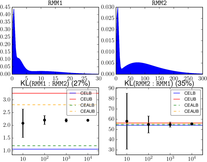
    𝚁𝙼𝙼1subscript𝚁𝙼𝙼1\mathtt{RMM}_{1}’s components, in the form (σi,wi)subscript𝜎𝑖subscript𝑤𝑖(\sigma_{i},w_{i}), are given by (0.5,1/3)0.513(0.5,1/3), (2,1/3)213(2,1/3), (10,1/3)1013(10,1/3); 𝚁𝙼𝙼2subscript𝚁𝙼𝙼2\mathtt{RMM}_{2} consists of (5,0.25)50.25(5,0.25), (60,0.25)600.25(60,0.25), (100,0.5)1000.5(100,0.5).

  3. 3.

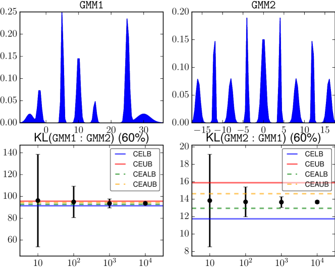
    𝙶𝙼𝙼1subscript𝙶𝙼𝙼1\mathtt{GMM}_{1}’s components, in the form (μi,σi,wi)subscript𝜇𝑖subscript𝜎𝑖subscript𝑤𝑖(\mu_{i},\sigma_{i},w_{i}), are (5,1,0.05)510.05(-5,1,0.05), (2,0.5,0.1)20.50.1(-2,0.5,0.1), (5,0.3,0.2)50.30.2(5,0.3,0.2), (10,0.5,0.2)100.50.2(10,0.5,0.2), (15,0.4,0.05)150.40.05(15,0.4,0.05) (25,0.5,0.3)250.50.3(25,0.5,0.3), (30,2,0.1)3020.1(30,2,0.1); 𝙶𝙼𝙼2subscript𝙶𝙼𝙼2\mathtt{GMM}_{2} consists of (16,0.5,0.1)160.50.1(-16,0.5,0.1), (12,0.2,0.1)120.20.1(-12,0.2,0.1), (8,0.5,0.1)80.50.1(-8,0.5,0.1), (4,0.2,0.1)40.20.1(-4,0.2,0.1), (0,0.5,0.2)00.50.2(0,0.5,0.2), (4,0.2,0.1)40.20.1(4,0.2,0.1), (8,0.5,0.1)80.50.1(8,0.5,0.1), (12,0.2,0.1)120.20.1(12,0.2,0.1)), (16,0.5,0.1)160.50.1(16,0.5,0.1).

  4. 4.

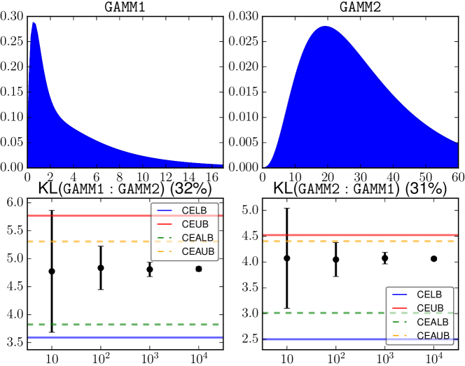
    𝙶𝚊𝙼𝙼1subscript𝙶𝚊𝙼𝙼1\mathtt{GaMM}_{1}’s components, in the form (ki,λi,wi)subscript𝑘𝑖subscript𝜆𝑖subscript𝑤𝑖(k_{i},\lambda_{i},w_{i}), are (2,0.5,1/3)20.513(2,0.5,1/3), (2,2,1/3)2213(2,2,1/3), (2,4,1/3)2413(2,4,1/3); 𝙶𝚊𝙼𝙼2subscript𝙶𝚊𝙼𝙼2\mathtt{GaMM}_{2} consists of (4,5,1/3)4513(4,5,1/3), (4,8,1/3)4813(4,8,1/3), (4,10,1/3)41013(4,10,1/3).

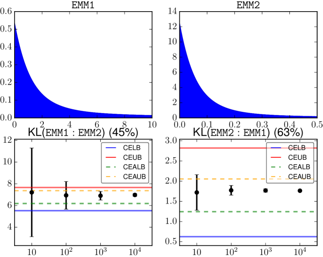
We compare the proposed bounds with Monte-Carlo estimation with different sample sizes in the range {10,102,103,104}10superscript102superscript103superscript104\{10,10^{2},10^{3},10^{4}\}. For each sample size configuration, Monte-Carlo estimation is repeated for 100 times to get the statistics. Fig. (3)(a-d) shows the input signals as well as the estimation results, where the proposed bounds CELB, CEUB, CEALB, CEAUB are presented as horizontal lines, and the Monto-Carlo estimations over different sample sizes are presented as error bars. We can loosely consider the average Monte-Carlo output with the largest sample size (104superscript10410^{4}) as the underlying truth, which is clearly inside our bounds. This serves as an empirical justification on the correctness of the bounds.

A key observation is that the bounds can be very tight, especially when the underlying KL divergence has a large magnitude, e.g. KL(𝚁𝙼𝙼2:𝚁𝙼𝙼1)\mathrm{KL}(\mathtt{RMM}_{2}:\mathtt{RMM}_{1}). This is because the gap between the lower and upper bounds is always guaranteed to be within logk+logk𝑘superscript𝑘\log{k}+\log{k}^{\prime}. Because KL is unbounded measure [9], in the general case two mixture models may have a large KL. Then our approximation gap is relatively very small. On the other hand, we also observed that the bounds in certain cases, e.g. KL(𝙴𝙼𝙼2:𝙴𝙼𝙼1)\mathrm{KL}(\mathtt{EMM}_{2}:\mathtt{EMM}_{1}), are not as tight as the other cases. When the underlying KL is small, the bound is not as informative as the general case.

Comparatively, there is a significant improvement of the data-dependent bounds (CEALB and CEAUB) over the combinatorial bounds (CELB and CEUB). In all investigated cases, the adaptive bounds can roughly shrink the gap by half of its original size at the cost of additional computation.

Note that, the bounds are accurate and must contain the true value. Monte-Carlo estimation gives no guarantee on where the true value is. For example, in estimating KL(𝙶𝙼𝙼1:𝙶𝙼𝙼2)\mathrm{KL}(\mathtt{GMM}_{1}:\mathtt{GMM}_{2}), Monte-Carlo estimation based on 103superscript10310^{3} samples can go beyond our bounds! It therefore suffers from a larger estimation error.

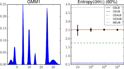
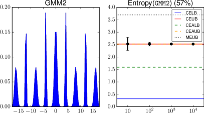
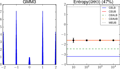
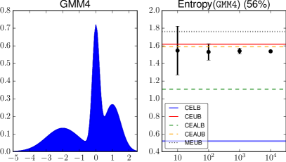
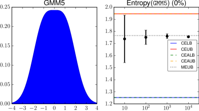
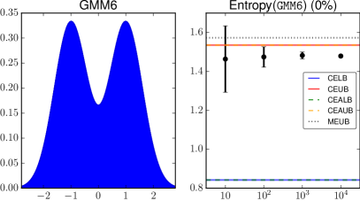
We simulates a set of Gaussian mixture models besides the above 𝙶𝙼𝙼1subscript𝙶𝙼𝙼1\mathtt{GMM}_{1} and 𝙶𝙼𝙼2subscript𝙶𝙼𝙼2\mathtt{GMM}_{2}. Fig. 4 shows the GMM densities as well as their differential entropy. A detailed explanation of the components of each GMM model is omitted for brevity.

The key observation is that CEUB (CEAUB) is very tight in most of the investigated cases. This is because that the upper envelope that is used to compute CEUB (CEAUB) gives a very good estimation of the input signal.

Notice that MEUB only gives an upper bound of the differential entropy as discussed in section 3. In general the proposed bounds are tighter than MEUB. However, this is not the case when the mixture components are merged together and approximate one single Gaussian (and therefore its entropy can be well apporiximated by the Gaussian entropy), as shown in the last line of Fig. 4.
Refer to caption
(a) KL divergence between two exponential mixture models
Refer to caption
(b) KL divergence between two Rayleigh mixture models
\phantomcaption
Refer to caption
(a) KL divergence between two Gaussian mixture models
Refer to caption
(b) KL divergence between two Gamma mixture models
Figure 3: Lower and upper bounds on the KL divergence between mixture models. The percentage in the title indicates the improvement of adaptive bounds (dashed lines) over the combinatorial bounds (solid lines). The error-bars show the means and standard deviations of KL (y-axis) by Monte-Carlo estimation using the corresponding sample size (x-axis).
Refer to caption Refer to caption
Figure 4: Lower and upper bounds on the differential entropy of Gaussian mixture models. On the left of each subfigure is the simulated GMM signal. On the right of each subfigure is the estimation of its differential entropy. Compared to Fig. 3, the Maximum Entropy Upper Bound shown by the black dotted line is added.

5 Concluding remarks and perspectives

We have presented a fast versatile method to compute bounds on the Kullback-Leibler divergence between mixtures by building algorithmically formula. We reported on our experiments for various mixture models in the exponential family. For univariate GMMs, we get a guaranteed bound of the KL divergence of two mixtures m𝑚m and msuperscript𝑚m^{\prime} with k𝑘k and ksuperscript𝑘k^{\prime} components within an additive approximation factor of logk+logk𝑘superscript𝑘\log k+\log k^{\prime} in O((k+k)log(k+k))𝑂𝑘superscript𝑘𝑘superscript𝑘O\left((k+k^{\prime})\log(k+k^{\prime})\right)-time. Therefore the larger the KL divergence the better the bound when considering a multiplicative (1+α)1𝛼(1+\alpha)-approximation factor since α=logk+logkKL(m:m)\alpha=\frac{\log k+\log k^{\prime}}{\mathrm{KL}(m:m^{\prime})}. The adaptive bounds is guaranteed to yield better bounds at the expense of computing potentially O(k2+(k)2)𝑂superscript𝑘2superscriptsuperscript𝑘2O\left(k^{2}+(k^{\prime})^{2}\right) intersection points of pairwise weighted components.

Our technique also yields bound for the Jeffreys divergence (the symmetrized KL divergence: J(m,m)=KL(m:m)+KL(m:m)J(m,m^{\prime})=\mathrm{KL}(m:m^{\prime})+\mathrm{KL}(m^{\prime}:m)) and the Jensen-Shannon divergence [19] (JS):

JS(m,m)=12(KL(m:m+m2)+KL(m:m+m2)),\mathrm{JS}(m,m^{\prime})=\frac{1}{2}\left(\mathrm{KL}\left(m:\frac{m+m^{\prime}}{2}\right)+\mathrm{KL}\left(m^{\prime}:\frac{m+m^{\prime}}{2}\right)\right),

since m+m2𝑚superscript𝑚2\frac{m+m^{\prime}}{2} is a mixture model with k+k𝑘superscript𝑘k+k^{\prime} components. One advantage of this statistical distance is that it is symmetric, always bounded by log22\log 2, and its square root yields a metric distance [13]. The log-sum-exp inequalities may also used to compute some Rényi divergences [26]:

Rα(m,p)=1α1log(m(x)αp(x)1α)dx,subscript𝑅𝛼𝑚𝑝1𝛼1𝑚superscript𝑥𝛼𝑝superscript𝑥1𝛼d𝑥R_{\alpha}(m,p)=\frac{1}{\alpha-1}\log\left(\int m(x)^{\alpha}p(x)^{1-\alpha}\right)\mathrm{d}x,

when α𝛼\alpha is an integer, m(x)𝑚𝑥m(x) a mixture and p(x)𝑝𝑥p(x) a single (component) distribution. Getting fast guaranteed tight bounds on statistical distances between mixtures opens many avenues. For example, we may consider building hierarchical mixture models by merging iteratively two mixture components so that those pair of components is chosen so that the KL distance between the full mixture and the simplified mixture is minimized.

In order to be useful, our technique is unfortunately limited to univariate mixtures: Indeed, in higher dimensions, we can still compute the maximization diagram of weighted components (an additively weighted Bregman Voronoi diagram [22, 4] for components belonging to the same exponential family). However, it becomes more complex to compute in the elementary Voronoi cells V𝑉V, the functions Ci,j(V)subscript𝐶𝑖𝑗𝑉C_{i,j}(V) and Mi(V)subscript𝑀𝑖𝑉M_{i}(V) (in 1D, the Voronoi cells are segments). We may obtain hybrid algorithms by approximating or estimating these functions. In 2D, it is thus possible to obtain lower and upper bounds on the Mutual Information [14] (MI) when the joint distribution m(x,y)𝑚𝑥𝑦m(x,y) is a 2D mixture of Gaussians:

I(M;M)=m(x,y)logm(x,y)m(x)m(y)dxdy.𝐼𝑀superscript𝑀𝑚𝑥𝑦𝑚𝑥𝑦𝑚𝑥superscript𝑚𝑦d𝑥d𝑦I(M;M^{\prime})=\int m(x,y)\log\frac{m(x,y)}{m(x)m^{\prime}(y)}\mathrm{d}x\mathrm{d}y.

Indeed, the marginal distributions m(x)𝑚𝑥m(x) and m(y)superscript𝑚𝑦m^{\prime}(y) are univariate Gaussian mixtures.

A Python code implementing those computational-geometric methods for reproducible research is available online at:

https://www.lix.polytechnique.fr/~nielsen/KLGMM/

Let us now conclude this work by noticing that the Kullback-Leibler of two smooth mixtures can be arbitrarily finely approximated by a Bregman divergence [2]. We loosely derive this observation using two different approaches:

  • Continuous mixture distributions have smooth densities that can be arbitrarily closely approximated using a single distribution (potentially multi-modal) belonging to the Polynomial Exponential Families [8, 27] (PEFs). A polynomial exponential family of order D𝐷D has log-likelihood l(x;θ)i=1Dθixiproportional-to𝑙𝑥𝜃superscriptsubscript𝑖1𝐷subscript𝜃𝑖superscript𝑥𝑖l(x;\theta)\propto\sum_{i=1}^{D}\theta_{i}x^{i}: Therefore, a PEF is an exponential family with polynomial sufficient statistics t(x)=(x,x2,,xD)𝑡𝑥𝑥superscript𝑥2superscript𝑥𝐷t(x)=(x,x^{2},\ldots,x^{D}). However, the log-normalizer FD(θ)=logexp(θt(x))dxsubscript𝐹𝐷𝜃superscript𝜃top𝑡𝑥differential-d𝑥F_{D}(\theta)=\log\int\exp(\theta^{\top}t(x))\mathrm{d}x of a D𝐷D-order PEF is not available in closed-form. Nevertheless, the KL of two mixtures m(x)𝑚𝑥m(x) and m(x)superscript𝑚𝑥m^{\prime}(x) can be theoretically approximated closely by a Bregman divergence: KL(m(x):m(x))KL(p(x;θ):p(x;θ))=BFD(θ:θ)\mathrm{KL}(m(x):m^{\prime}(x))\simeq\mathrm{KL}(p(x;\theta):p(x;\theta^{\prime}))=B_{F_{D}}(\theta^{\prime}:\theta), where θ𝜃\theta and θsuperscript𝜃\theta^{\prime} are the natural parameters of the PEF family {p(x;θ)}𝑝𝑥𝜃\{p(x;\theta)\} approximating m(x)𝑚𝑥m(x) and m(x)superscript𝑚𝑥m^{\prime}(x), respectively (i.e., m(x)p(x;θ)similar-to-or-equals𝑚𝑥𝑝𝑥𝜃m(x)\simeq p(x;\theta) and m(x)p(x;θ)similar-to-or-equalssuperscript𝑚𝑥𝑝𝑥superscript𝜃m^{\prime}(x)\simeq p(x;\theta^{\prime})).

  • Consider two finite mixtures m(x)=i=1kwipi(x)𝑚𝑥superscriptsubscript𝑖1𝑘subscript𝑤𝑖subscript𝑝𝑖𝑥m(x)=\sum_{i=1}^{k}w_{i}p_{i}(x) and m(x)=j=1kwjpj(x)superscript𝑚𝑥superscriptsubscript𝑗1superscript𝑘superscriptsubscript𝑤𝑗superscriptsubscript𝑝𝑗𝑥m^{\prime}(x)=\sum_{j=1}^{k^{\prime}}w_{j}^{\prime}p_{j}^{\prime}(x) of k𝑘k and ksuperscript𝑘k^{\prime} components (possibly with heterogeneous components pi(x)subscript𝑝𝑖𝑥p_{i}(x)’s and pj(x)superscriptsubscript𝑝𝑗𝑥p_{j}^{\prime}(x)’s), respectively. In information geometry, a mixture family is the set of convex combination of fixed333Thus in statistics, a mixture is understood as a convex combination of parametric components while in information geometry a mixture family is the set of convex combination of fixed components. component densities. Let us consider the mixture families {g(x;(w,w))}𝑔𝑥𝑤superscript𝑤\{g(x;(w,w^{\prime}))\} generated by the D=k+k𝐷𝑘superscript𝑘D=k+k^{\prime} fixed components p1(x),,pk(x),p1(x),,pk(x)subscript𝑝1𝑥subscript𝑝𝑘𝑥superscriptsubscript𝑝1𝑥superscriptsubscript𝑝superscript𝑘𝑥p_{1}(x),\ldots,p_{k}(x),p_{1}^{\prime}(x),\ldots,p_{k^{\prime}}^{\prime}(x):

    {g(x;(w,w))=i=1kwipi(x)+j=1kwjpj(x):i=1kwi+j=1kwj=1}conditional-set𝑔𝑥𝑤superscript𝑤superscriptsubscript𝑖1𝑘subscript𝑤𝑖subscript𝑝𝑖𝑥superscriptsubscript𝑗1superscript𝑘superscriptsubscript𝑤𝑗superscriptsubscript𝑝𝑗𝑥superscriptsubscript𝑖1𝑘subscript𝑤𝑖superscriptsubscript𝑗1superscript𝑘superscriptsubscript𝑤𝑗1\left\{g(x;(w,w^{\prime}))=\sum_{i=1}^{k}w_{i}p_{i}(x)+\sum_{j=1}^{k^{\prime}}w_{j}^{\prime}p_{j}^{\prime}(x)\ :\ \sum_{i=1}^{k}w_{i}+\sum_{j=1}^{k^{\prime}}w_{j}^{\prime}=1\right\}

    We can approximate arbitrarily finely mixture m(x)𝑚𝑥m(x) for any ϵ>0italic-ϵ0\epsilon>0 by g(x;α)(1ϵ)m(x)+ϵm(x)similar-to-or-equals𝑔𝑥𝛼1italic-ϵ𝑚𝑥italic-ϵsuperscript𝑚𝑥g(x;\alpha)\simeq(1-\epsilon)m(x)+\epsilon m^{\prime}(x) with α=((1ϵ)w,ϵw)𝛼1italic-ϵ𝑤italic-ϵsuperscript𝑤\alpha=((1-\epsilon)w,\epsilon w^{\prime}) (so that i=1k+kαi=1superscriptsubscript𝑖1𝑘superscript𝑘subscript𝛼𝑖1\sum_{i=1}^{k+k^{\prime}}\alpha_{i}=1) and m(x)g(x;α)=ϵm(x)+(1ϵ)m(x)similar-to-or-equalssuperscript𝑚𝑥𝑔𝑥superscript𝛼italic-ϵ𝑚𝑥1italic-ϵsuperscript𝑚𝑥m^{\prime}(x)\simeq g(x;\alpha^{\prime})=\epsilon m(x)+(1-\epsilon)m^{\prime}(x) with α=(ϵw,(1ϵ)w)superscript𝛼italic-ϵ𝑤1italic-ϵsuperscript𝑤\alpha^{\prime}=(\epsilon w,(1-\epsilon)w^{\prime}) (and i=1k+kαi=1superscriptsubscript𝑖1𝑘superscript𝑘superscriptsubscript𝛼𝑖1\sum_{i=1}^{k+k^{\prime}}\alpha_{i}^{\prime}=1). Therefore KL(m(x):m(x))KL(g(x;α):g(x;α))=BF(α:α)\mathrm{KL}(m(x):m^{\prime}(x))\simeq\mathrm{KL}(g(x;\alpha):g(x;\alpha^{\prime}))=B_{F^{*}}(\alpha:\alpha^{\prime}), where F(α)=g(x;α)logg(x;α)dxsuperscript𝐹𝛼𝑔𝑥𝛼𝑔𝑥𝛼differential-d𝑥F^{*}(\alpha)=\int g(x;\alpha)\log g(x;\alpha)\mathrm{d}x is the Shannon information (negative Shannon entropy) for the composite mixture family. Interestingly, this Shannon information can be arbitrarily closely approximated when considering isotropic Gaussians [21]. Notice that the convex conjugate F(θ)𝐹𝜃F(\theta) of the continuous Shannon neg-entropy F(η)superscript𝐹𝜂F^{*}(\eta) is the log-sum-exp function on the inverse soft map.

Appendix A The Kullback-Leibler divergence of mixture models is not analytic [34]

Ideally, we aim at getting a finite length closed-form formula to compute the KL divergence of mixture models. But this is provably mathematically intractable because of the log-sum term in the integral, as we shall prove below. Analytic expressions encompass closed-form formula and include special functions (e.g., Gamma function) but do not allow to use limits nor integrals. An analytic function f(x)𝑓𝑥f(x) is a Csuperscript𝐶C^{\infty} function (infinitely differentiable) such that at any point x0subscript𝑥0x_{0} its k𝑘k-order Taylor series Tk(x)=i=0kf(i)(x0)i!(xx0)isubscript𝑇𝑘𝑥superscriptsubscript𝑖0𝑘superscript𝑓𝑖subscript𝑥0𝑖superscript𝑥subscript𝑥0𝑖T_{k}(x)=\sum_{i=0}^{k}\frac{f^{(i)}(x_{0})}{i!}(x-x_{0})^{i} converges to f(x)𝑓𝑥f(x): limkTk(x)=f(x)subscript𝑘subscript𝑇𝑘𝑥𝑓𝑥\lim_{k\rightarrow\infty}T_{k}(x)=f(x) for x𝑥x belonging to a neighborhood Nr(x0)={x:|xx0|r}subscript𝑁𝑟subscript𝑥0conditional-set𝑥𝑥subscript𝑥0𝑟N_{r}(x_{0})=\{x:|x-x_{0}|\leq r\} of x0subscript𝑥0x_{0} where r𝑟r is called the radius of convergence. The analytic property of a function is equivalent to the condition that for each k𝑘k\in\mathbb{N}, there exists a constant c𝑐c such that |dkfdxk(x)|ck+1k!superscriptd𝑘𝑓dsuperscript𝑥𝑘𝑥superscript𝑐𝑘1𝑘\left|\frac{\mathrm{d}^{k}f}{\mathrm{d}x^{k}}(x)\right|\leq c^{k+1}k!.

To prove that the KL of mixtures is not analytic (hence does not admit a closed-form formula), we shall adapt the proof reported in [34] (in Japanese444We thank Professor Aoyagi for sending us his paper [34].). We shall prove that KL(p:q)\mathrm{KL}(p:q) is not analytic for univariate mixtures of densities p(x)=G(x;0,1)𝑝𝑥𝐺𝑥01p(x)=G(x;0,1) and q(x;w)=(1w)G(x;0,1)+wG(x;1,1)𝑞𝑥𝑤1𝑤𝐺𝑥01𝑤𝐺𝑥11q(x;w)=(1-w)G(x;0,1)+wG(x;1,1) for w(0,1)𝑤01w\in(0,1), where G(x;μ,σ)=12πσexp((xμ)22σ2)𝐺𝑥𝜇𝜎12𝜋𝜎superscript𝑥𝜇22superscript𝜎2G(x;\mu,\sigma)=\frac{1}{\sqrt{2\pi}\sigma}\exp(-\frac{(x-\mu)^{2}}{2\sigma^{2}}) is the density of a univariate Gaussian of mean μ𝜇\mu and standard deviation σ𝜎\sigma. Let D(w)=KL(p(x):q(x;w))D(w)=\mathrm{KL}(p(x):q(x;w)) denote the divergence between these two mixtures (p𝑝p has a single component and q𝑞q has two components).

We have logp(x)q(x;w)=log(1+w(ex121))𝑝𝑥𝑞𝑥𝑤1𝑤superscript𝑒𝑥121\log\frac{p(x)}{q(x;w)}=-\log(1+w(e^{x-\frac{1}{2}}-1)), and

dkDdwk=(1)kkp(x)(ex121)dx.superscriptd𝑘𝐷dsuperscript𝑤𝑘superscript1𝑘𝑘𝑝𝑥superscript𝑒𝑥121differential-d𝑥\frac{\mathrm{d}^{k}D}{\mathrm{d}w^{k}}=\frac{(-1)^{k}}{k}\int p(x)(e^{x-\frac{1}{2}}-1)\mathrm{d}x.

Let x0subscript𝑥0x_{0} be the root of the equation ex121=ex2superscript𝑒𝑥121superscript𝑒𝑥2e^{x-\frac{1}{2}}-1=e^{\frac{x}{2}} so that for xx0𝑥subscript𝑥0x\geq x_{0}, we have ex121ex2superscript𝑒𝑥121superscript𝑒𝑥2e^{x-\frac{1}{2}}-1\geq e^{\frac{x}{2}}. It follows that:

|dkDdwk|1kx0p(x)ekx2dx=1kek28Aksuperscriptd𝑘𝐷dsuperscript𝑤𝑘1𝑘superscriptsubscriptsubscript𝑥0𝑝𝑥superscript𝑒𝑘𝑥2differential-d𝑥1𝑘superscript𝑒superscript𝑘28subscript𝐴𝑘\left|\frac{\mathrm{d}^{k}D}{\mathrm{d}w^{k}}\right|\geq\frac{1}{k}\int_{x_{0}}^{\infty}p(x)e^{\frac{kx}{2}}\mathrm{d}x=\frac{1}{k}e^{\frac{k^{2}}{8}}A_{k}

with Ak=x012πexp(xk22)dxsubscript𝐴𝑘superscriptsubscriptsubscript𝑥012𝜋𝑥𝑘22differential-d𝑥A_{k}=\int_{x_{0}}^{\infty}\frac{1}{\sqrt{2\pi}}\exp(-\frac{x-\frac{k}{2}}{2})\mathrm{d}x. When k𝑘k\rightarrow\infty, we have Ak1subscript𝐴𝑘1A_{k}\rightarrow 1. Consider k0subscript𝑘0k_{0}\in\mathbb{N} such that Ak0>0.9subscript𝐴subscript𝑘00.9A_{k_{0}}>0.9. Then the radius of convergence r𝑟r is such that:

1rlimk(1kk!0.9exp(k28))1k=.1𝑟subscript𝑘superscript1𝑘𝑘0.9superscript𝑘281𝑘\frac{1}{r}\geq\lim_{k\rightarrow\infty}\left(\frac{1}{kk!}0.9\exp\left(\frac{k^{2}}{8}\right)\right)^{\frac{1}{k}}=\infty.

Thus the convergence radius is r=0𝑟0r=0, and therefore the KL divergence is not an analytic function of the parameter w𝑤w. The KL of mixtures is an example of a non-analytic smooth function. (Notice that the absolute value is not analytic at 00.)

Appendix B Closed-form formula for the Kullback-Leibler divergence between scaled and truncated exponential families

When computing approximation bounds for the KL divergence between two mixtures m(x)𝑚𝑥m(x) and m(x)superscript𝑚𝑥m^{\prime}(x), we end up with the task of computing 𝒟wapa(x)logwbpb(x)wcpc(x)dxsubscript𝒟subscript𝑤𝑎subscript𝑝𝑎𝑥superscriptsubscript𝑤𝑏superscriptsubscript𝑝𝑏𝑥superscriptsubscript𝑤𝑐superscriptsubscript𝑝𝑐𝑥d𝑥\int_{\mathcal{D}}w_{a}p_{a}(x)\log\frac{w_{b}^{\prime}p_{b}^{\prime}(x)}{w_{c}^{\prime}p_{c}^{\prime}(x)}\mathrm{d}x where 𝒟𝒳𝒟𝒳\mathcal{D}\subseteq\mathcal{X} is a subset of the full support 𝒳𝒳\mathcal{X}. We report a generic formula for computing these formula when the mixture (scaled and truncated) components belong to the same exponential family [23]. An exponential family has canonical log-density written as l(x;θ)=logp(x;θ)=θt(x)F(θ)+k(x)𝑙𝑥𝜃𝑝𝑥𝜃superscript𝜃top𝑡𝑥𝐹𝜃𝑘𝑥l(x;\theta)=\log p(x;\theta)=\theta^{\top}t(x)-F(\theta)+k(x), where t(x)𝑡𝑥t(x) denotes the sufficient satistics, F(θ)𝐹𝜃F(\theta) the log-normalizer (also called cumulant function or partition function), and k(x)𝑘𝑥k(x) an auxiliary carrier term.

Let KL(w1p1:w2p2:w3p3)=𝒳w1p1(x)logw2p2(x)w3p3(x)dx=H×(w1p1:w3p3)H×(w1p1:w2p2)\mathrm{KL}(w_{1}p_{1}:w_{2}p_{2}:w_{3}p_{3})=\int_{\mathcal{X}}w_{1}p_{1}(x)\log\frac{w_{2}p_{2}(x)}{w_{3}p_{3}(x)}\mathrm{d}x={H_{\times}}(w_{1}p_{1}:w_{3}p_{3})-{H_{\times}}(w_{1}p_{1}:w_{2}p_{2}). Since it is a difference of two cross-entropies, we get for three distributions belonging to the same exponential family [25] the following formula:

KL(w1p1:w2p2:w3p3)=w1logw2w3+w1(F(θ3)F(θ2)(θ3θ2)F(θ1)).\mathrm{KL}(w_{1}p_{1}:w_{2}p_{2}:w_{3}p_{3})=w_{1}\log\frac{w_{2}}{w_{3}}+w_{1}(F(\theta_{3})-F(\theta_{2})-(\theta_{3}-\theta_{2})^{\top}\nabla F(\theta_{1})).

Furthermore, when the support is restricted, say to support range 𝒟𝒳𝒟𝒳\mathcal{D}\subseteq\mathcal{X}, let m𝒟(θ)=𝒟p(x;θ)dxsubscript𝑚𝒟𝜃subscript𝒟𝑝𝑥𝜃differential-d𝑥m_{\mathcal{D}}(\theta)=\int_{\mathcal{D}}p(x;\theta)\mathrm{d}x denote the mass and p(x;θ)~=p(x;θ)m𝒟(θ)~𝑝𝑥𝜃𝑝𝑥𝜃subscript𝑚𝒟𝜃\tilde{p(x;\theta)}=\frac{p(x;\theta)}{m_{\mathcal{D}}(\theta)} the normalized distribution. Then we have:

𝒟w1p1(x)logw2p2(x)w3p3(x)dx=m𝒟(θ1)(KL(w1p~1:w2p~2:w3p~3))logw2m𝒟(θ3)w3m𝒟(θ2).\int_{\mathcal{D}}w_{1}p_{1}(x)\log\frac{w_{2}p_{2}(x)}{w_{3}p_{3}(x)}\mathrm{d}x=m_{\mathcal{D}}(\theta_{1})(\mathrm{KL}(w_{1}\tilde{p}_{1}:w_{2}\tilde{p}_{2}:w_{3}\tilde{p}_{3}))-\log\frac{w_{2}m_{\mathcal{D}}(\theta_{3})}{w_{3}m_{\mathcal{D}}(\theta_{2})}.

When F𝒟(θ)=F(θ)logm𝒟(θ)subscript𝐹𝒟𝜃𝐹𝜃subscript𝑚𝒟𝜃F_{\mathcal{D}}(\theta)=F(\theta)-\log m_{\mathcal{D}}(\theta) is strictly convex and differentiable then p(x;θ)~~𝑝𝑥𝜃\tilde{p(x;\theta)} is an exponential family and the closed-form formula follows straightforwardly. Otherwise, we still get a closed-form but need more derivations. For univariate distributions, we write 𝒟=(a,b)𝒟𝑎𝑏\mathcal{D}=(a,b) and m𝒟(θ)=abp(x;θ)dx=Pθ(b)Pθ(a)subscript𝑚𝒟𝜃superscriptsubscript𝑎𝑏𝑝𝑥𝜃differential-d𝑥subscript𝑃𝜃𝑏subscript𝑃𝜃𝑎m_{\mathcal{D}}(\theta)=\int_{a}^{b}p(x;\theta)\mathrm{d}x=P_{\theta}(b)-P_{\theta}(a) where Pθ(a)=ap(x;θ)dxsubscript𝑃𝜃𝑎superscript𝑎𝑝𝑥𝜃differential-d𝑥P_{\theta}(a)=\int^{a}p(x;\theta)\mathrm{d}x denotes the cumulative distribution function.

The usual formula for truncated and scaled Kullback-Leibler divergence is:

KL𝒟(wp(x;θ):wp(x;θ))=wm𝒟(θ)(logww+BF(θ:θ))+w(θθ)m𝒟(θ),\mathrm{KL}_{\mathcal{D}}(wp(x;\theta):w^{\prime}p(x;\theta^{\prime}))=wm_{\mathcal{D}}(\theta)\left(\log\frac{w}{w^{\prime}}+B_{F}(\theta^{\prime}:\theta)\right)+w{(\theta^{\prime}-\theta)}^{\top}{\nabla m_{\mathcal{D}}(\theta)}, (22)

where BF(θ:θ)B_{F}(\theta^{\prime}:\theta) is a Bregman divergence [3]:

BF(θ:θ)=F(θ)F(θ)(θθ)F(θ).B_{F}(\theta^{\prime}:\theta)=F(\theta^{\prime})-F(\theta)-(\theta^{\prime}-\theta)^{\top}\nabla F(\theta).

This formula extends the classic formula [3] for full regular exponential families (by setting w=w=1𝑤superscript𝑤1w=w^{\prime}=1 and m𝒟(θ)=1subscript𝑚𝒟𝜃1m_{\mathcal{D}}(\theta)=1 with m𝒟(θ)=0subscript𝑚𝒟𝜃0\nabla m_{\mathcal{D}}(\theta)=0).

Similar formula are available for the cross-entropy and entropy of exponential families [25].

References

  • [1] Shun-ichi Amari. Information Geometry and Its Applications, volume 194. Springer, 2016.
  • [2] Arindam Banerjee, Srujana Merugu, Inderjit S Dhillon, and Joydeep Ghosh. Clustering with Bregman divergences. The Journal of Machine Learning Research, 6:1705–1749, 2005.
  • [3] Arindam Banerjee, Srujana Merugu, Inderjit S Dhillon, and Joydeep Ghosh. Clustering with Bregman divergences. Journal of machine learning research, 6(Oct):1705–1749, 2005.
  • [4] Jean-Daniel Boissonnat, Frank Nielsen, and Richard Nock. Bregman Voronoi diagrams. Discrete & Computational Geometry, 44(2):281–307, 2010.
  • [5] Manuel Bronstein. Symbolic integration. I. , Transcendental functions. Algorithms and computation in mathematics. Springer, Berlin, 2005.
  • [6] Giuseppe C. Calafiore and Laurent El Ghaoui. Optimization models. Cambridge university press, 2014.
  • [7] Miguel A. Carreira-Perpinan. Mode-finding for mixtures of Gaussian distributions. IEEE Transactions on Pattern Analysis and Machine Intelligence, 22(11):1318–1323, 2000.
  • [8] Loren Cobb, Peter Koppstein, and Neng Hsin Chen. Estimation and moment recursion relations for multimodal distributions of the exponential family. Journal of the American Statistical Association, 78(381):124–130, 1983.
  • [9] Thomas M Cover and Joy A Thomas. Elements of information theory. John Wiley & Sons, 2012.
  • [10] Mark De Berg, Marc Van Kreveld, Mark Overmars, and Otfried Cheong Schwarzkopf. Computational geometry. Springer, 2000.
  • [11] Olivier Devillers and Mordecai J Golin. Incremental algorithms for finding the convex hulls of circles and the lower envelopes of parabolas. Information Processing Letters, 56(3):157–164, 1995.
  • [12] Jean-Louis Durrieu, Jean-Philippe Thiran, and Finnian Kelly. Lower and upper bounds for approximation of the Kullback-Leibler divergence between Gaussian mixture models. In IEEE International Conference on Acoustics, Speech and Signal Processing (ICASSP), pages 4833–4836. Ieee, 2012.
  • [13] Dominik M Endres and Johannes E Schindelin. A new metric for probability distributions. Information Theory, IEEE Transactions on, 49(7):1858–1860, 2003.
  • [14] David V Foster and Peter Grassberger. Lower bounds on mutual information. Physical Review E, 83(1):010101, 2011.
  • [15] Zhi-Kai Huang and Kwok-Wing Chau. A new image thresholding method based on Gaussian mixture model. Applied Mathematics and Computation, 205(2):899–907, 2008.
  • [16] Marco F Huber, Tim Bailey, Hugh Durrant-Whyte, and Uwe D Hanebeck. On entropy approximation for Gaussian mixture random vectors. In Multisensor Fusion and Integration for Intelligent Systems, 2008. MFI 2008. IEEE International Conference on, pages 181–188. IEEE, 2008.
  • [17] Simon J Julier, Tim Bailey, and Jeffrey K Uhlmann. Using exponential mixture models for suboptimal distributed data fusion. In Nonlinear Statistical Signal Processing Workshop, 2006 IEEE, pages 160–163. IEEE, 2006.
  • [18] Erik Learned-Miller and Joseph DeStefano. A probabilistic upper bound on differential entropy. IEEE Transactions on Information Theory, 54(11):5223–5230, 2008.
  • [19] Jianhua Lin. Divergence measures based on the Shannon entropy. Information Theory, IEEE Transactions on, 37(1):145–151, 1991.
  • [20] Joseph V Michalowicz, Jonathan M Nichols, and Frank Bucholtz. Calculation of differential entropy for a mixed Gaussian distribution. Entropy, 10(3):200–206, 2008.
  • [21] Kamyar Moshksar and Amir K. Khandani. Arbitrarily tight bounds on differential entropy of gaussian mixtures. IEEE Transactions on Information Theory, 62(6):3340–3354, June 2016.
  • [22] Frank Nielsen, Jean-Daniel Boissonnat, and Richard Nock. On bregman Voronoi diagrams. In Proceedings of the eighteenth annual ACM-SIAM symposium on Discrete algorithms, pages 746–755. Society for Industrial and Applied Mathematics, 2007.
  • [23] Frank Nielsen and Vincent Garcia. Statistical exponential families: A digest with flash cards. arXiv preprint arXiv:0911.4863, 2009.
  • [24] Frank Nielsen and Richard Nock. Entropies and cross-entropies of exponential families. In 17th IEEE International Conference on Image Processing (ICIP), pages 3621–3624. IEEE, 2010.
  • [25] Frank Nielsen and Richard Nock. Entropies and cross-entropies of exponential families. In IEEE International Conference on Image Processing, pages 3621–3624. IEEE, 2010.
  • [26] Frank Nielsen and Richard Nock. On Rényi and Tsallis entropies and divergences for exponential families. arXiv preprint arXiv:1105.3259, 2011.
  • [27] Frank Nielsen and Richard Nock. Patch matching with polynomial exponential families and projective divergences. In 9th International Conference Similarity Search and Applications (SISAP), 2016.
  • [28] Frank Nielsen and Mariette Yvinec. An output-sensitive convex hull algorithm for planar objects. International Journal of Computational Geometry & Applications, 8(01):39–65, 1998.
  • [29] Olivier Schwander, Stéphane Marchand-Maillet, and Frank Nielsen. Comix: Joint estimation and lightspeed comparison of mixture models. In 2016 IEEE International Conference on Acoustics, Speech and Signal Processing, ICASSP 2016, Shanghai, China, March 20-25, 2016, pages 2449–2453, 2016.
  • [30] José Seabra, Francesco Ciompi, Oriol Pujol, Josepa Mauri, Petia Radeva, and Joao Sanches. Rayleigh mixture model for plaque characterization in intravascular ultrasound. Biomedical Engineering, IEEE Transactions on, 58(5):1314–1324, 2011.
  • [31] Ophir Setter, Micha Sharir, and Dan Halperin. Constructing two-dimensional Voronoi diagrams via divide-and-conquer of envelopes in space. Springer, 2010.
  • [32] Micha Sharir and Pankaj K. Agarwal. Davenport-Schinzel sequences and their geometric applications. Cambridge University Press, Cambridge, New York, 1995.
  • [33] Chunhua Shen and Hanxi Li. On the dual formulation of boosting algorithms. Pattern Analysis and Machine Intelligence, IEEE Transactions on, 32(12):2216–2231, 2010.
  • [34] Sumio Watanabe, Keisuke Yamazaki, and Miki Aoyagi. Kullback information of normal mixture is not an analytic function. Technical report of IEICE (in Japanese), pages 41–46, 2004.
  • [35] Makoto Yamada and Masashi Sugiyama. Direct importance estimation with Gaussian mixture models. IEICE transactions on information and systems, 92(10):2159–2162, 2009.