Matter localization on brane-worlds generated by deformed defects
Abstract
Abstract
Localization and mass spectrum of bosonic and fermionic matter fields of some novel families of asymmetric thick brane configurations generated by deformed defects are investigated. The localization profiles of spin 0, spin 1/2 and spin 1 bulk fields are identified for novel matter field potentials supported by thick branes with internal structures. The condition for localization is constrained by the brane thickness of each model such that thickest branes strongly induces matter localization. The bulk mass terms for both fermion and boson fields are included in the global action as to produce some imprints on mass-independent potentials of the Kaluza-Klein modes associated to the corresponding Schrödinger equations. In particular, for spin 1/2 fermions, a complete analytical profile of localization is obtained for the four classes of superpotentials here discussed. Regarding the localization of fermion fields, our overall conclusion indicates that thick branes produce a left-right asymmetric chiral localization of spin 1/2 particles.
pacs:
11.25.Mj, 04.40.Nr, 11.10.KkI Introduction
The brane-world model is a prominent paradigm that has been addressed to solve several questions in physics. Within this framework, brane-worlds are required to render a consistent 4D physics of our Universe, at least up to certain sensible limits Arkani02 . In the brane-world scenario all kinds of matter fields should be localized on the brane. In the RS brane-world model Randall , the brane is generated by a scalar field coupled to gravity DeWolfe ; Gremm , in a particular scenario which may be interpreted as the thin brane limit of thick brane scenarios. Generically, a prominent test that thick brane-world models must pass, to be physically consistent, regards their stability, with respect to tensor, vector, and scalar fluctuations of the background fields that generate the field configurations, namely, the thick brane itself. At least the zero modes of Standard Model matter fields were shown to be localized on several brane-world models Liu0907.0910 ; Liu_20101 ; Zhang ; Andrianov:2013vqa ; Folomeev ; Brane , suggesting that such kind of models are physically viable in high energy physics. Several alternative scenarios, including Gauss-Bonnet terms, gravity, tachyonic potentials, cyclic defects, and Bloch branes, have been further studied German:2012rv ; German:2013sk ; Bernardini ; ddutra , and analogous scenarios in an expanding Universe have been approached Ahmed ; Bernardini:2014vba . The curvature nature of the brane-world, namely, to be a de Sitter, Minkowski or anti-de Sitter one, is in general obtained a posteriori, by solving the 5D Einstein field equations. In fact, the bulk and the brane cosmological constants depend upon the brane and the bulk gravitational field content, governed by curvature, and must obey the intrinsic fine-tuning, in the Randall-Sundrum-like models limit.
The analytical study of stability can be uncontrollably intricate, due to the involved structure of the scalar field coupled to gravity. To circumvent the complicated and not analytical approaches, linearized formulations have been commonly worked out. In this context, supported by the stability of deformed defect generated brane-world models, scalar, vector, and tensor perturbations are investigated throughout this work.
Localization aspects of various matter fields with spin 0, 1/2, and 1 on analytical thick brane-world models are indeed a main concern in deriving brane-world models, since they must describe our physical world. The localization of the spin 1/2 fermions deserves a special attention, since there is no scalar field to couple with in this model, in contrast to thick branes generated by deforming defect mechanisms Barbosa-Cendejas:2015qaa . Otherwise, Kalb-Ramond fields, although already investigated Cruz:2013zka , shall not be the main aim here. The spin 1/2 issue has been previously studied in some other contexts PRD_Oda_026002 , including further coupling of more scalar fields in the action casana and asymmetric brane-worlds generated by a plenty of scalar field potentials bazeiamr ; Bazeia:2012qh ; Guo:2011qt ; Dutra:2013jea ; Liu0907.0910 . In particular, asymmetric Bloch branes in the context of the hierarchy problem have been addressed in Ref. ddutra .
Our aim is to investigate the localization of bulk matter and gauge fields on the brane, in the context where the mass-independent potentials of the corresponding Schrödinger-like equations, regarding the 1 quantum mechanical analogue problem, can be suitably acquired from a warped metric. In particular, for a bulk mass proportional to the fermion mass term enclosed by the global action, the possibility of trapping spin 1/2 fermions on asymmetric branes is discussed and quantified.
To accomplish this aim, this paper is organized as follows. In Sect. II, a brief review of brane-world scenarios supported by an effective action driven by a (dark sector) scalar field is presented. Warp factors and the corresponding internal brane structure are described for four different analytical models. In Sect. III, the left-right chiral asymmetric aspects of matter localization for spin 1/2 fermion fields on thick branes are investigated. Extensions to scalar boson and vector boson fields are obtained in Sect. IV and V, respectively. Final conclusions are drawn in Sect. VI.
II Brane-world preliminaries and some analytical models
Let one starts considering a space-time warped into . The most general metric compatible with a brane-world spatially flat cosmological background has the form given by
| (1) |
where denotes the warp factor, and the signature is employed, with . The stands for the components of the metric tensor (). One can identify as the infinite extra-dimension coordinate (which runs from to ), and notice that the normal to surfaces of constant is orthogonal to the brane, into the bulk 111Brane tension terms have been suppressed/absorbed by the metric (c. f. Eqs. (24) and (25) from Ref. Folomeev for real scalar field Lagrangians in the context of thick brane solutions)..
The brane-world scenario examined here is setup by an effective action, driven by a (dark sector) scalar field, , coupled to gravity, given by
| (2) |
where is the scalar curvature, is the Ricci tensor, and denotes the 5D gravitational coupling constant, hereon set to equal to unity, where is the 5D Newton constant. The Einstein equations read
| (3) |
where denotes the energy-momentum tensor corresponding to the matter Lagrangian, regarding the matter field . After solving the 5D Einstein field equations, the bulk cosmological constant turns out, in general, to be positive or negative, thus realising a de Sitter or anti-de Sitter brane-world, respectively, generated by curvature. It realises and emulates the interplay involving the 4D and 5D cosmological constants. Some further possibilities are devised, e. g., in German:2012rv ; HerreraAguilar:2010kt , however it is worth to mention that an additional scalar field can be still added in the action, whose isotropisation shall precisely define the nature of the brane-world. This the latter case is however beyond the scope of our analysis. Obviously, whatever the possibility to be considered, the thin brane limit must obey the fine-tuning relation maartens , among the effective 4D and 5D cosmological constants and the brane tension as well.
Considering the real scalar field action, Eq. (2), one can compute the stress-energy tensor
| (4) |
which, supposing that both the scalar field and the warp factor dynamics depend only upon the extra coordinate, , leads to an explicit dependence of the energy density in terms of the field, , and of its first derivative, , as
| (5) |
With the same constraints on about the dependence on , the equations of motion currently known from DeWolfe ; Gremm , which arise from the above action, are
| (6) |
through a variational principle relative to the scalar field, , and
| (7) |
through a variational principle relative to the metric, or equivalently to , manipulated to result into
| (8) |
after an integration over .
For the scalar field potential written in terms of a superpotential, , as
| (9) |
the above equations are mapped into first-order equations DeWolfe ; Gremm as
| (10) |
and
| (11) |
for which the solutions can be found straightforwardly through immediate integrations DeWolfe (see also Ref. Folomeev and references therein). The energy density follows from Eq. (9) as
| (12) |
The analysis of localization aspects of brane-world scenarios shall be constrained by some known examples, , , and , for which the warp factor, , and the energy density, , can be analytically computed. The model is supported by a sine-Gordon-like superpotential given by
| (13) |
which reproduces the results from Ref. Gremm . The model corresponds to a deformed theory with the superpotential given by
| (14) |
Models and are deformed topological solutions from Ref. Bernardini13 supported by superpotentials like
| (15) |
and
| (16) |
where the parameter fixes the thickness of the brane described by the warp factor, . Besides exhibiting analytically manipulable profiles, the above superpotentials have already been discussed in the context of thick brane localization Gremm ; Brane ; Folomeev . The models and are respectively motivated by sine-Gordon and theories, and models and are obtained (also analytically) from deformed versions of the model Bernardini . In particular, models and can also be mapped onto tachyonic Lagrangian versions of scalar field brane models Bernardini13 ; Zhang ; Folomeev .
From the above superpotentials, the respective solutions for are set as
| (17) | |||||
| (18) | |||||
| (19) | |||||
| (20) |
where one has suppressed any additional (irrelevant) constant of integration for convenience, and one has just considered the positive solutions 222In Eqs. (17)-(20) there could let be explicit a constant of integration that amounts to letting , corresponding to the position of the brane in the extra dimension, for which one has set ..
The obtained expressions for the warp factor as resulting from Eq. (11) are respectively given by
| (21) | |||||
| (22) | |||||
| (23) | |||||
| (24) |
where integration constants are introduced as to set a normalization criterium for which .
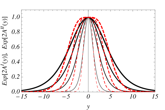
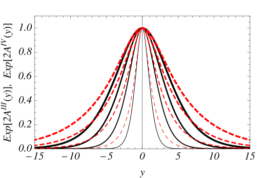
The solutions for and are depicted in Fig. 1. The corresponding localized energy densities computed through Eq. (12) are respectively given by
| (25) | |||||
| (26) | |||||
| (27) | |||||
| (28) |
The brane scenarios for models from to are depicted in Fig. (1) for the warp factors and in Fig. (2) for the energy densities, from which one can observe that models from to give rise to thick branes, most of them with no internal structures. In fact, only the potential that controls the scalar field from model allows the emergence of thick branes that host internal structures in the form of a layer of a novel phase enclosed by two separate interfaces, inside which the energy density of the matter field gets more concentrated. It is related to the extension/localization of the warp factor, namely when the profiles depicted in Fig. (1) approach to a plateu form in the region very inside of the brane, the corresponding internal structure is observed through its energy profile.
The appearance of negative energy densities in the plots for may be related to a predominance of the scalar field potential over the kinetic-like term related to the coordinate . Speculatively, it indicates that the vacuum minimal energy can be adjusted by the inclusion of some additional term, eventually related to the cosmological constant.
The localization of bulk matter fields on thick branes generated by each one of these models shall be identified in the following sections. Spin 0, spin 1/2, and spin 1 fields shall evolve coupled to gravity and, as usual, the bulk matter field contribution to the bulk energy shall be neglected. It means that the obtained solutions hold in the presence of the bulk matter, without disturbing the bulk geometry.
III Asymmetric left-right matter localization for spin 1/2 fermion fields
To investigate the localization of bulk matter on the brane, one first considers that fermion localization on brane-worlds is usually accomplished when the Dirac algebra is realized by the objects , where denotes the fünfbein, the satisfy the Clifford relation , and are the gamma matrices in the flat spacetime. Hereupon and denote the and local Lorentz indexes, respectively. The fünfbein is provided by , where , and and are respectively the gamma matrices and the volume element, respectively. The Dirac action for a spin 1/2 fermion with a mass term can be expressed as PRD_Oda_026002 ; Guo:2011qt
| (29) |
Here is the spin connection, where
and is some general scalar function, providing a mass term with a kink-like profile, which from this point is written in terms of a conformal variable such that regards a transformation to conformal coordinates. This kind of mass term is introduced in the action, for it has played a critical role on the localization of fermionic fields on a Minkowski brane. The components of the spin connection with respect to (1) are where is the spin connection derived from the metric . Thus, the equation of motion corresponding to the action (29) reads
| (30) |
The Dirac equation can be hence studied by taking spinors with respect to effective fields. In this way the chiral splitting yields
| (31) |
where and are the well-known KK modes, and [] is the right-chiral [left-chiral] component of a Dirac field, respectively. In addition, the sum over can be both continuous and discrete. Assuming that , the and functions should then satisfy the subsequent coupled equations,
| (32a) | |||||
| (32b) | |||||
The associated Schrödinger-like equations can be thus acquired for the left and right-chiral KK modes of fermions, respectively, as:
| (33) | |||||
| (34) |
where the mass-independent potentials are given by
| (35a) | |||||
| (35b) | |||||
Note that the Schrödinger-like equations (33) and (34) can be transformed into and , where . This observation is based upon supersymmetric quantum mechanics, implying that the mass squared is non-negative.
In order to lead these results to the standard action for a massless fermion, and a series of massive chiral fermions, the action is employed, for orthonormalization conditions
| (36) |
If in the formulae (32a) and (32b), by setting thus it yields
| (37) |
Hence, either the massless left- or right-chiral KK fermion modes can be localized on the brane, being the another one non-normalizable.
By taking , regarding Eqs. (17)-(20), it yields
| (38a) | |||||
| (38b) | |||||
Eqs. (38a) and (38b), evince that, when the mass term in the action (29) regards , the potentials for left and right-chiral KK modes vanish. Then both chiral fermions cannot be localized on the thick brane. Moreover, if and are demanded to be -even with respect to the extra dimension , then the mass term must be an odd function of Liu:2013kxz . In fact, some useful classes of brane-world models have the extra dimension topology . If the background scalar is an odd function of extra warped dimension, the Yukawa coupling, between the fermion and the background scalar field, assures the localization mechanism for fermions Liu:2013kxz . For the majority brane-world models, the scalar field is, usually, a kink, being an odd function of the extra dimension. Here we do not necessarily impose this condition, in order to not preclude asymmetric solutions, with respect to the extra dimension.
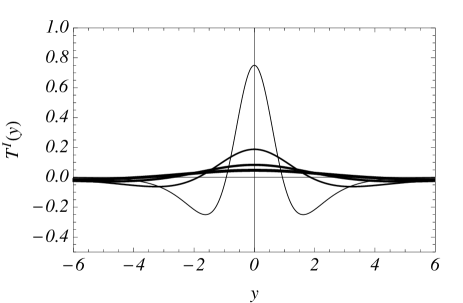
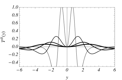
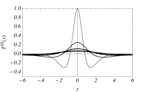
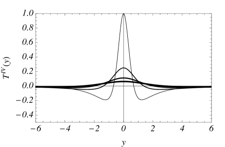
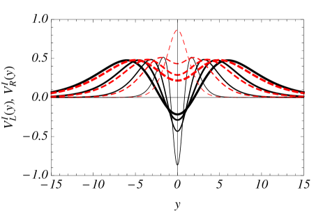
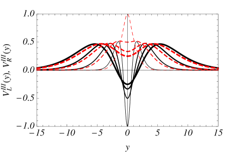
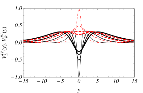
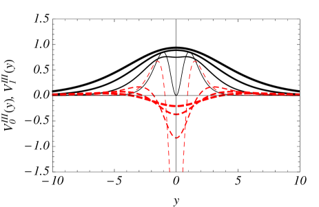
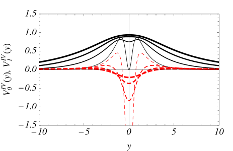
In what follows the profile of the above left-right potentials is depicted in Fig. (3) for different values of the localization parameter . In fact, the potentials have asymptotic behaviors that tend to zero from up, as , for all models from to . In the model , at the potential attains its maximum positive value, a global maximum, for . The potential changes to a volcano-type profile along the interval of , such that for the point regards a local minima, which allows for producing unstable resonances, which can be tunneled to the outside of the potential. Nevertheless, the potential has the associated minima at for all positive integer values of , , and it creates the conditions for producing bound states. A very similar behavior is exhibited by the model , in spite of showing different amplitudes. The model is quite similar to these models, with the only qualitative difference concerning that, at , the potential attains its maximum positive value, a global maximum, for and . For the model , the stability conditions created by the right- and left- chiral volcano-type potentials are more sensible to the increasing of the brane width (), in comparison to models and ones (), inducing no mass gap to separate the fermion zero mode from the excited KK massive modes. In these cases, there exist continuous spectra for the Kaluza-Klein modes of fermions of both chiralities. These volcano-type potentials imply into the existence of resonant or metastable states of fermions which can tunnel from the brane to the bulk Liu_20101 . The left-chiral KK mode has a continuous gapless spectrum for the models , , and , according to Fig. (3). Since the potential for left-chiral fermions presents a negative value at the brane location for these models, the zero mode of right- and left-chiral fermions, and are the only necessary ingredient to be tested to be localized on the brane. For the model , both potentials for the left- and right-chiral fermions have positive values of the potential, irrespectively of . However for, in both cases, i. e. for , when , an asymmetric behavior emerges and produces a totally odd symmetric well-barrier profile in the limit of . Except for , the zero mode of left- and right-chiral fermions can not be trapped. All potentials for the model are asymmetric (except for , which is nonsense in the brane context), have maxima at and tends to zero at , and there is no bound state for right-chiral fermions. In particular, for when , the minima occur at .
IV Matter localization for spin 0 scalar fields
The localization of scalar fields on thick branes generated by deformed defects can also be considered from this point. In particular, an interesting approach on domain walls can be also found in Ref. PRD_Stojkovic . In fact, a massive scalar field coupled to gravity can be described by the following action,
| (39) |
where denotes the effective mass of a bulk scalar field, , and from where one can check whether spin 0 matter fields can be trapped on the thick brane. By employing the metric (1), the associated equation of motion from the action in Eq. (39) reads
| (40) |
Hence, by the KK decomposition , where is assumed to satisfy the Klein-Gordon equation being the mass of the KK excitation of the scalar field. Then the scalar KK mode is ruled by the following equation:
| (41) |
This equation is a Schrödinger one, with effective potential given by
| (42) |
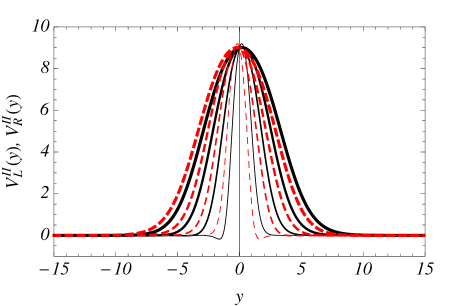
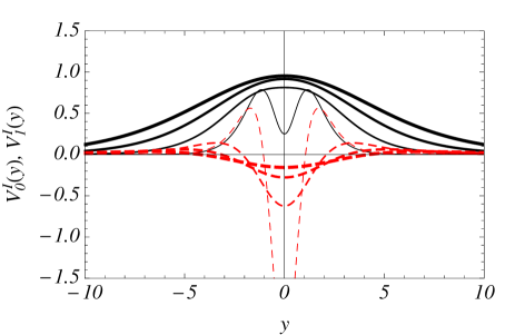
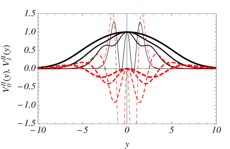
The profile of the above scalar boson potential is depicted in Fig. (4) (solid (black) lines) for different values of the localization parameter . For , only brane scenarios with provide conditions to have a localized scalar field. Even in this case, such localized states behave much more as resonances than as bound states, given that it can be tunneled out of the potential. Bound states appear only for non integer values of the brane width such that , which shall correspond to typical volcano-type potentials.
V Matter localization for spin 1 vector fields
One now turns to spin 1 vector fields and begins with the action of a vector field
| (43) |
where denotes the field strength tensor. A spin 1 field can be now studied via the KK decomposition The action of the massless vector field (43) is invariant under the following gauge transformation:
| (44) |
where denotes any arbitrary regular scalar function, for . The field component equals zero Guo:2011qt , by this gauge. In fact, Eq. (44) yields
| (45) |
By choosing Guo:2011qt then , hence the action (43) is led to the spacetime action
| (46) |
where . Given a set of orthonormal functions , playing the role of spin 1 Kaluza-Klein modes, and the decomposition of the vector field , the action (46) reads
where stands for the field strength tensor. The KK modes satisfy the Schrödinger equation
where the mass-independent potential reads guo
| (47) |
The profile of the above vector boson potential is depicted in Fig. (4) (dashed (red) lines) for different values of the localization parameter . All the thick brane scenarios with provide localization conditions to have vector field bound states. Increasing values of lead to more stable bound states.
VI Conclusions and discussion
Thick branes driven by superpotentials supported by deformed defects (c. f. Eqs. (13)-(16)), for various bulk matter fields of spin 0, spin 1/2, and spin 1 have been investigated. For spin 1 gauge fields, the profile of the associated vector boson potential showed that, in the thick brane models for , localization conditions hold as to guarantee the existence of vector field bound states. Quantitatively, increasing values of the brane thickness parameter, , leads to more stable bound states.
Concerning spin 0 (scalar) fields, the profile of the potential evinces that only thick brane scenarios with provide localization conditions compatible to scalar field bound states.
The most intricate result is related to spin 1/2 fields. In fact, for fermionic fields, left-right potentials were deeply studied and for the four models considered here, the issue of localization has been scrutinized. It is worth to point out that models , , and admit volcano-type potentials, inducing no mass gap to separate the fermion zero mode from the excited KK massive modes. Hence a continuous spectra for the Kaluza-Klein modes of fermions of both chiralities are allowed. A refined analysis of the values of the parameter in these models, influencing the localization of fermionic fields, was provided. The model , induced by the superpotential (14), reveals a peculiar behavior. In this model, right-chiral fermions have positive values of the potential irrespectively of the extra dimension when . Hence, except for this value, the zero mode of left- and right-chiral fermions can not be trapped. All potentials for the model are asymmetric, have maxima at and minima at , and there is no bound state for right-chiral fermions, but, again, for when .
It is worth to mention that, for the localization of a fermion zero mode, the mass term was considered in the action. An interesting approach concerning such mass term in Eq. (29) has been studied, corresponding to the so-called singular dark spinors Ahluwalia:2009rh ; daRocha:2011yr . Such massive mass dimension one quantum fields are prime candidates for the dark matter problem, also presenting possible signatures at LHC Dias:2010aa . It generates a slightly different action responsible for spin 1/2 matter fields localization Liu:2011nb ; Jardim:2014xla . Such approach can be also extended in the context of deformed defects here presented.
Acknowledgement
Acknowledgments - The work of AEB is supported by the Brazilian Agencies FAPESP (grant 2015/05903-4) and CNPq (grant No. 300809/2013-1 and grant No. 440446/2014-7). RdR is grateful to CNPq (grants No. 303293/2015-2, and No. 473326/2013-2), and to FAPESP (grant 2015/10270-0) for partial financial support.
References
- (1) I. Antoniadis, N. Arkani-Hamed, S. Dimopoulos and G. Dvali, Phys. Lett. B 436, 257 (1998).
- (2) L. Randall and R. Sundrum, Phys. Rev. Lett. 83, 3370 (1999).
- (3) O. DeWolfe, D. Z. Freedman, S. S. Gubser and A. Karch, Phys. Rev. D 62, 046008 (2000).
- (4) M. Gremm, Phys. Lett. B 478, 434 (2000).
- (5) D. Bazeia, C. Furtado and A. R. Gomes, JCAP 0402, 002 (2004).
- (6) X. H. Zhang, Y. X. Liu and Y. S. Duan, Mod. Phys. Lett. A 23, 2093 (2008).
- (7) A. A. Andrianov, V. A. Andrianov and O. O. Novikov, Eur. Phys. J. C 73, 2675 (2013).
- (8) Y.-X. Liu, C.-E. Fu, L. Zhao and Y.-S. Duan, Phys. Rev. D 80, 065020 (2009).
- (9) A. Herrera-Aguilar, D. Malagon-Morejon and R. R. Mora-Luna, JHEP 1011, 015 (2010).
- (10) R. Maartens, K. Koyama, Brane-world gravity, Living Rev. Rel. 13, 5 (2010).
- (11) Z.-H. Zhao, Y.-X. Liu, H.-T. Li and Y.-Q. Wang, Phys. Rev. D 82, 084030 (2010).
- (12) V. Dzhunushaliev, V. Folomeev and M. Minamitsuji, Rep. Prog. Phys. 73, 066901 (2010).
- (13) A. E. Bernardini and R. da Rocha, Adv. High Energy Phys. 2013, 304980 (2013).
- (14) R. A. C. Correa, A. de Souza Dutra and M. B. Hott, Class. Quant. Grav. 28, 155012 (2011).
- (15) G. German, A. Herrera-Aguilar, D. Malagon-Morejon, R. R. Mora-Luna and R. da Rocha, JCAP 1302, 035 (2013).
- (16) G. German, A. Herrera–Aguilar, D. Malagon–Morejon, I. Quiros and R. da Rocha, Phys. Rev. D 89, 026004 (2014).
- (17) A. E. Bernardini, R. T. Cavalcanti and R. da Rocha, Gen. Rel. Grav. 47, 1840 (2015).
- (18) A. Ahmed and B. Grzadkowski, JHEP 1301, 177 (2013).
- (19) N. Barbosa-Cendejas, D. Malag on-Morejo n and R. R. Mora-Luna, Gen. Relat. Grav. 47, 77 (2015).
- (20) W. T. Cruz, R. V. Maluf and C. A. S. Almeida, Eur. Phys. J. C 73, 2523 (2013).
- (21) I. Oda, Phys. Rev. D 64, 026002 (2001).
- (22) C. A. S. Almeida, R. Casana, M. M. Ferreira and A. R. Gomes, Phys. Rev. D 79, 125022 (2009).
- (23) D. Bazeia, R. Menezes and R. da Rocha, Adv. High Energy Phys. 2014, 276729 (2014).
- (24) D. Bazeia, L. Losano, R. Menezes and R. da Rocha, Eur. Phys. J. C 73, 2499 (2013).
- (25) A. de Souza Dutra, G. P. de Brito and J. M. Hoff da Silva, Europhys. Lett. 108, 11001 (2014).
- (26) H. Guo, A. Herrera-Aguilar, Y. X. Liu, D. Malagon-Morejon and R. R. Mora-Luna, Phys. Rev. D 87, 095011 (2013).
- (27) D. Stojkovic, Phys. Rev. D 63, 025010 (2000).
- (28) A. E. Bernardini and O. Bertolami, Phys. Lett. B 726, 512 (2013).
- (29) Y. X. Liu, Z. G. Xu, F. W. Chen and S. W. Wei, Phys. Rev. D 89, 086001 (2014).
- (30) D. V. Ahluwalia, C. Y. Lee and D. Schritt, Phys. Rev. D 83, 065017 (2011).
- (31) R. da Rocha, A. E. Bernardini and J. M. Hoff da Silva, JHEP 1104, 110 (2011).
- (32) M. Dias, F. de Campos and J. M. Hoff da Silva, Phys. Lett. B 706, 352 (2012).
- (33) I. C. Jardim, G. Alencar, R. R. Landim and R. N. Costa Filho, Phys. Rev. D 91, 085008 (2015).
- (34) Y. X. Liu, X. N. Zhou, K. Yang and F. W. Chen, Phys. Rev. D 86, 064012 (2012).
- (35) Q.-Y. Xie, Z.-H. Zhao, Y. Zhong, J. Yang, X.-N. Zhou, JCAP 1503, 014 (2015).