Lower Bounds on Parameter Modulation–Estimation Under Bandwidth Constraints

Abstract

We consider the problem of modulating the value of a parameter onto a band-limited signal to be transmitted over a continuous-time, additive white Gaussian noise (AWGN) channel, and estimating this parameter at the receiver. The performance is measured by the mean power-$\alpha$ error (MP$\alpha$E), which is defined as the worst-case $\alpha$-th order moment of the absolute estimation error. The optimal exponential decay rate of the MP$\alpha$E as a function of the transmission time, is investigated. Two upper (converse) bounds on the MP$\alpha$E exponent are derived, on the basis of known bounds for the AWGN channel of inputs with unlimited bandwidth. The bounds are computed for typical values of the error moment and the signal-to-noise ratio (SNR), and the SNR asymptotics of the different bounds are analyzed. The new bounds are compared to known converse and achievability bounds, which were derived from channel coding considerations.

I Introduction

The problem of waveform communication, as termed in the classic book by Wozencraft and Jacobs [1, Chapter 8], is about conveying the value of a continuous valued parameter to a distant location, via a communication channel. Formally, at the input of the channel, a modulator maps a parameter $u\in[0,1)$ to a signal $\{s(t,u),\;0\leq t\leq T\}$, which is transmitted over the continuous-time AWGN channel, under a power constraint, $\frac{1}{T}\int_{0}^{T}s^{2}(t,u)\mathrm{d}t\leq P$. At the output of the channel, an estimator processes the received signal, $y(t)=s(t,u)+z(t),\;0\leq t\leq T$, to obtain an estimate of the parameter. Here, $z(t)$ is a Gaussian white noise process with two-sided spectral density $\nicefrac{{N_{0}}}{{2}}$.

Such a modulation-estimation system can be depicted in a geometrical way, as shown in Fig. 1. As noticed by Kotel’inkov [2] and Shannon [3],

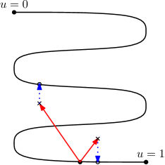
Figure 1: The signal space with a locus obtained from a Shannon-Kotel’inkov mapping [3, Fig. 4]. As the parameter exhausts the interval $[0,1)$, the point on the signal space travels from the top left point of the locus to its bottom right point. Dots corresponds to actual parameter values. The solid (red) arrows represent the effect of the noise, and the circles represent estimated parameter values. The dotted (blue) arrows represent the estimation stage.

the various signals $\{s(t,u),\;0\leq u<1\}$ can be represented as vectors in some signal space. The modulator can therefore be viewed as mapping the parameter into a point in the signal space, and as the parameter exhausts its domain, a locus (possibly, discontinuous) in the signal space is obtained. The additive noise then shifts the transmitted point to a different point in the signal space, and the estimator maps it back to a point on the locus, which in turn corresponds to an estimated value of the parameter. The estimation performance is usually evaluated by the $\alpha$-th order moment of the absolute estimation error, which we term the mean power-$\alpha$ error (MP$\alpha$E). Most commonly, the mean square error (MSE) is used ($\alpha=2$). As can be discerned from Fig. 1, the estimation error can be roughly categorized into two types: (i) weak noise errors, which result in small estimation errors, and are associated with the local, linearized behavior of the locus (right red arrow in Fig. 1), and (ii) anomalous errors, that yield relatively large estimation errors, which are associated with the twisted curvature of the locus in the signal space for non-linear modulation systems (left red arrow in Fig. 1). A good communication system should properly balance between the two types of errors. Nonetheless, when the SNR falls below a certain threshold, the anomalous error quickly dominates and the MP$\alpha$E becomes catastrophic. This phenomenon is known as the threshold effect, see, e.g., [1, 4], and many references therein.

A natural question, for such systems, is how small can the MP$\alpha$E be made for an arbitrary modulation-estimation system, operating over transmission time $T$? As usual, answering this question exactly is prohibitively complex, even in very low dimensions [2, 5]. However, it turns out that if the modulator and estimator are designed carefully, the MP$\alpha$E may decay exponentially with $T$, to wit

$$\sup_{u\in[0,1)}\mathbb{E}_{u}\left\{\left|\hat{U}-u\right|^{\alpha}\right\}\approx e^{-E\cdot T}$$ (1)

for some constant $E>0$, where $\hat{U}$ is the estimator and $\mathbb{E}_{u}\{\cdot\}$ is the expectation operator with respect to (w.r.t.) the channel noise, when the underlying parameter is $u$. As we next review, the optimal exponential decay rate of the MP$\alpha$E was investigated, in the same spirit that the optimal exponential decay of the error probability was studied for the problem of channel coding (e.g. [6, Chapter 5] and [7, Chapter 10]).

Most of the previous research has focused on the AWGN channel without bandwidth constraints on the input signals. The goal of this paper is to develop bounds on the MP$\alpha$E for band-limited input signals, with emphasis on lower bounds. Since a lower bound on the MP$\alpha$E is associated with an upper bound on its exponent and vice-versa, then to avoid confusion, throughout the paper the term ‘converse bound’ will be used in the sense of an upper bound on the MP$\alpha$E exponent. Similarly, the term ‘achievability bound’ will be used for a lower bound on the MP$\alpha$E exponent. Nevertheless, the terms ‘converse’ and ‘achievability’ are only used here in a loose way, in the sense that it does not necessarily imply that the lower bound on the exponent coincides with the upper bound.

We begin with a short review on existing bounds for the continuous-time, unlimited-bandwidth case. For achievability results, a few simple systems were considered. In [1, Chapter 8], a frequency position modulation (FPM) system with a central frequency and bandwidth that both increase exponentially with $T$, i.e., as $\exp(RT)$, for some optimized $R$, was shown to achieve an exponential decrease of the MSE according to $\exp(-\frac{P}{3N_{0}}T)$. In the same spirit, a pulse position modulation (PPM) can be used, again, with exponentially increasing bandwidth, to achieve the same exponent. More recently, a modulation scheme which employs uniform quantization of the parameter to $\exp(RT)$ values (where $R>0$ is again a design parameter), followed by an optimal rate-$R$ channel code for AWGN channel (i.e., its reliability function), was shown to achieve the same exponent (see [8, Introduction]). A similar system will be discussed in Section III.

To assess the performance of the above schemes, converse bounds have also been derived. On the face of it, as this problem lies in the intersection between information theory and estimation theory, methods from both fields are expected to have the potential to provide answers. While estimation theory offers an ample of Bayesian and non-Bayesian bounds [9] (see also [10, Introduction] and references therein for an overview), the vast majority of them strongly depend on the specific modulator, and so, they are less useful for us in the quest for universal bounds, i.e., when there is freedom to optimize the modulator. From the information-theoretic perspective, one can view the parameter as an information source, and assume that it is a random variable $U$, say, distributed uniformly over $[0,1)$. The estimate $\hat{U}$, is then chosen to minimize the average distortion, under a distortion measure defined as the $\alpha$-th order moment of the absolute error. The MP$\alpha$E is then the average distortion $D$ of this joint source-channel coding system, and, in principle, the data processing theorem (DPT) [11, Section 7.13] can be harnessed to obtain a converse bound of the form $D\geq R^{-1}(C)$, where $R(D)$ is the rate-distortion function of the source and $C$ is the channel capacity. However, this bound may be too optimistic, since to achieve this bound using a separation-based system, the source should be compressed at a rate close to its rate-distortion function, which is impossible when there is merely a single source symbol (scalar quantization).

In the unlimited-bandwidth case, $C=\frac{P}{N_{0}}$, and while the rate-distortion function is not known to have a closed form formula, it can be lower bounded using Shannon’s lower bound (e.g. [12, Corollary 7.7.5], [13, Section 4.3.3]) as

$$R(D)\geq h(U)-\frac{1}{2}\log(2\pi eD)=-\frac{1}{2}\log(2\pi eD)$$ (2)

where $h(U)=0$ is the differential entropy of $U$. Therefore, the DPT lends itself to obtain a lower bound on the MSE, given by

$$D=\mathbb{E}(U-\hat{U})^{2}\geq\frac{1}{2\pi e}\exp(-2CT)=\frac{1}{2\pi e}\exp\left(-\frac{2P}{N_{0}}T\right).$$ (3)

In [14, Section 6] the idea of using a DPT with generalized information measures [15], which pertain to a general univariate convex function, was extended to multivariate convex functions, and harvested in order to obtain the improved bound of the exponential order of $\exp(-\frac{P}{N_{0}}T)$.

In a different line of work, a more direct approach was taken, and a lower bound on the MP$\alpha$E was developed from an analysis of the channel coding system introduced above, namely, a modulation system which maps a quantized value of the parameter to a codeword from a channel code (or a signal from a signal set). Rather complicated arguments were used to obtain a converse bound which is valid for any signal set. Research in this direction was initiated by Cohn in his Ph.D. thesis [16], who derived a lower bound of the exponential order $\exp(-\frac{P}{2.89\cdot N_{0}}T)$ for the MSE ($\alpha=2$). Later on, Burnashev [17, 18] has revised and generalized Cohn’s arguments, and his efforts eventually culminated in [18, Theorem 3], which provides, among other results, the lower exponential bound of the exponential order of $\exp(-\frac{P}{3N_{0}}T)$ for $\alpha=2$. As this converse bound coincides exponentially with the achievability bound, then the optimal exponent is precisely characterized for the unlimited-bandwidth AWGN channel.

The exploration of universal bounds to modulation-estimation problem was not confined only to AWGN channels and the MP$\alpha$E. In [19, Section IV], a large deviations performance metric was considered, namely, the exponential behavior of the probability that the estimation error would exceed some threshold. This exponent was fully characterized in [8]: For an optimal communication system, the probability that the absolute estimation error would exceed $\exp(-RT)$ behaves exponentially as $\exp[-T\cdot E(R)]$, where $E(R)$ is the reliability function of the channel.

The exponential behavior of the MP$\alpha$E discussed above for continuous-time channels, holds when there is no limitation on the bandwidth of the input signals. In [20], a converse bound and an achievability bound on exponent of the MP$\alpha$E were derived, for a discrete memoryless channel (in discrete-time), rather than the AWGN channel (in continuous-time). In this paper, we consider the problem of characterizing the maximal achievable exponent of the MP$\alpha$E for the AWGN channel fed by a band-limited input, with emphasis on converse bounds. We are not aware of earlier works that focus concretely on this setting.

As a simple benchmark, the DPT bound mentioned above can be adapted to input signals band-limited to $W$, by simply replacing the capacity of the unlimited-bandwidth case with the capacity of AWGN channel with band-limited inputs, i.e.,

$$C=W\log\left(1+\frac{P}{N_{0}W}\right).$$ (4)

The resulting lower bound on the MP$\alpha$E has exponential order of

$$\exp\left[-T\cdot\alpha W\log\left(1+\frac{P}{N_{0}W}\right)\right].$$ (5)

Thus, unlike the unlimited-bandwidth case, for which the MP$\alpha$E scales linearly with $\frac{P}{N_{0}}$, for the band-limited case, it only scales logarithmically with $\frac{P}{N_{0}}$.

In this paper, we improve on the converse bound of (5) using two different mechanisms. In the first, channel coding considerations, as the ones used in the converse bound of [20], will be used to derive a converse bound to the problem at hand. In the second method, we utilize the results of the unlimited-bandwidth case from [16, 17, 18], in a somewhat indirect way, rather than revising the complicated bounding techniques used to prove them. The general idea is to begin with a band-limited system, and transform it, by some means, to a new system. We will then relate the MP$\alpha$E exponent of the new system to the MP$\alpha$E exponent of the original system, and use the converse bound of the unlimited-bandwidth case, for the new system. This, in turn, will provide a converse bound on the original, band-limited system. Two new bounds will be derived from this general methodology. It turns out that none of the three converse bounds mentioned above dominates the other two, and for each of these bounds, there exists a region in the plane of the variables $\alpha$ and SNR such that this is the best bound out of the three.

To assess the tightness of the converse bounds, we will briefly discuss also achievability bounds. Specifically, the achievability bound of [20] will be adapted to the AWGN channel, just as the converse bound of [20] was. We will also speculate on a possible approach for improving this achievability bound, based on unequal error protection (even though, thus far, we were not able to demonstrate that it actually improves). It should be mentioned, that for this problem, converse bounds which are based on other, well-known, estimation-theoretic lower bounds, such as the Weiss-Weinstein bound [21, 22], have failed to provide stronger bounds, at least in the various ways we have tried to harness them.

The rest of the paper is organized as follows. In Section II, the modulation-estimation problem is formulated, and known results for the unlimited-bandwidth AWGN channel are reviewed. In Section III, the converse bound adapted from [20] is presented, and our main results, which are the two new converse bounds on the MP$\alpha$E exponent. The achievability bound, also adapted from [20], is discussed as well. In Section IV, the various converse bounds are compared to each other, as well as to the achievability bound. Numerical results are displayed, and a systematic comparison between the bounds is made, based on asymptotic SNR analysis.

II System Model and Background

Throughout the paper, real random variables will be denoted by capital letters, and specific values they may take will be denoted by the corresponding lower case letters. Random vectors and their realizations will be denoted, respectively, by capital letters and the corresponding lower case letters, both in the bold face font. Real random processes will be denoted by capital letters with a time argument, and specific sample paths will be denoted by the corresponding lower case letters. For example, the random vector $\mathbf{X}=(X_{1},\ldots,X_{N})$, ($N$ positive integer) may take a specific vector value $\mathbf{x}=(x_{1},\ldots,x_{N})$, and the random process $X(t)$ may have the sample path $x(t)$. The probability of an event ${\cal E}$, for an underlying parameter $u\in[0,1)$, will be denoted by $\mathbb{P}_{u}[{\cal E}]$, and the expectation operator will be denoted by $\mathbb{E}_{u}[\cdot]$. The indicator for a set ${\cal A}$ will be denoted by $\mathbb{I}\{{\cal A}\}$. Logarithms and exponents will be understood to be taken to the natural base. For the sake of brevity, for large integers, we will ignore integer constraints throughout, as they do not have any effect on the results. For example, we will assume a blocklength $N=2WT$, rather than $N=\left\lceil 2WT\right\rceil$, provided that $2WT\gg 1$.

Let $u\in[0,1)$ be a parameter and consider the continuous-time AWGN channel

$$y(t)=s(t,u)+z(t),$$ (6)

where $s(t,u)$ and $y(t)$ are the channel input and output, respectively, at time $t$, and $\{z(t)\}$ is a white Gaussian noise process with two-sided spectral density $\frac{N_{0}}{2}$.

Figure 2: A Modulation-estimation system.

A modulation-estimation system ${\cal S}_{T}$ of time duration $T$ is defined by a modulator and an estimator. The modulator maps a parameter value $u$ to a signal $\{s(t,u),\;0\leq t\leq T\}$, where $s(t,u)=0$ for $t<0$ and $t>T$, and where the mapping $u\to s(t,u)$ is assumed measurable. The estimator maps the received signal $\{y(t),\;0\leq t\leq T\}$ to an estimated parameter, $\hat{u}$. The system ${\cal S}_{T}$ is power-limited to $P$ if

$$\frac{1}{T}\int_{0}^{T}s^{2}(t,u)\cdot\mathrm{d}t\leq P$$ (7)

for all $u\in[0,1)$. The system is considered band-limited to $W$ if there exists an orthonormal basis of $N\triangleq 2WT$ functions $\{\phi_{n}(t),\;0\leq t\leq T\}_{n=1}^{N}$, such that for all $u\in[0,1)$, there exists a vector of coefficients, $\mathbf{s}(u)\triangleq(s_{1}(u),\ldots,s_{N}(u))$, such that

$$s(t,u)=\sum_{n=1}^{N}s_{n}(u)\cdot\phi_{n}(t),\quad 0\leq t\leq T.$$ (8)

Following a procedure similar to that of [12, Section 2.1], the continuous-time channel can be converted to an equivalent $N$-dimensional channel. As discussed there, the projections

$$y_{n}\triangleq\int_{0}^{T}y(t)\cdot\phi_{n}(t)\cdot\mathrm{d}t,\quad 1\leq n\leq N,$$ (9)

are sufficient statistics for the estimation of $u$. We may define the noise projections

$$z_{n}\triangleq\int_{0}^{T}z(t)\cdot\phi_{n}(t)\cdot\mathrm{d}t,\quad 1\leq n\leq N,$$ (10)

and group the projections into vectors, $\mathbf{y}=(y_{1},\ldots,y_{N})$ and $\mathbf{z}=(z_{1},\ldots,z_{N})$, to obtain an equivalent vector model

$$\mathbf{y}\triangleq\mathbf{s}(u)+\mathbf{z}.$$ (11)

In this model, the power constraint is given by $\left\|\mathbf{s}(u)\right\|^{2}\leq PT$, but for the purpose of converse bounds, it can be assumed, without loss of generality (w.l.o.g.), that the constraint is satisfied with equality. Indeed, as was discussed in [18, p. 249], [23, pp. 291-292], if $\left\|\mathbf{s}(u)\right\|^{2}<PT$ for some $u$, then a single dummy coordinate can be appended to $\{\mathbf{s}(u)\}$, which will make $\left\|\mathbf{s}(u)\right\|=PT$. For $N\gg 1$, this additional coordinate has a negligible effect on the time or bandwidth of the signals, and, in fact, can be totally ignored by the estimator. Regarding the noise, as the projection in (10) is performed on an orthogonal set, the resulting projections are independent, and thus $\mathbf{Z}\sim{\cal N}(\mathbf{0},\frac{N_{0}}{2}\cdot I_{N})$, where $I_{N}$ is the identity matrix of dimension $N$. The estimator, based on the channel (11), can then be denoted as a function of $\mathbf{y}$, i.e., $\hat{u}(\mathbf{y})$ rather than $\hat{u}\{y(t),\;0\leq t\leq T\}$ for (6).

At this point, a justification for adopting (11) as a proper model for a physically band-limited channel is required. The correspondence between the continuous-time model (6) and the discrete-frequency model (11) is a delicate, yet a mature subject. In short, signals cannot be both strictly time-limited and strictly band-limited. Thus, the basis functions $\{\phi_{n}(t),\;0\leq t\leq T\}_{n=1}^{N}$ are chosen to span the linear space of signals of duration $T$ exactly, and a bandwidth of approximately $W$. If $N=2WT\gg 1$, the proximity of the real bandwidth to $W$ can be made arbitrarily sharp. A detailed discussion can be found in [24, 25], and [6, Chapter 8].

For $\alpha>0$ (not necessarily integer), the mean power-$\alpha$ error (MP$\alpha$E) of ${\cal S}_{T}$ is defined as

$$e_{\alpha}({\cal S}_{T})\triangleq\sup_{u\in[0,1)}\mathbb{E}_{u}\left\{\left|\hat{u}(\mathbf{Y})-u\right|^{\alpha}\right\},$$ (12)

where $\mathbf{Y}$ is the random counterpart of $\mathbf{y}$. As we shall see, $e_{\alpha}({\cal S}_{T})$ can be made exponentially decreasing with $T$, and so, it is natural to ask what is the fastest possible exponential rate of decrease. Specifically, we say that $E$ is an achievable MP$\alpha$E exponent if there exists a family $\{{\cal S}_{T}\}$ of modulation-estimation systems, parametrized by $T$, such that

$$\limsup_{T\to\infty}\left[-\frac{1}{T}\cdot\log e_{\alpha}({\cal S}_{T})\right]\geq E.$$ (13)

The objective of the paper is to derive converse bounds on $E_{\alpha}(\nicefrac{{P}}{{N_{o}}},W)$, which is defined as the largest achievable MP$\alpha$E exponent, for a given power constraint $P$, bandwidth constraint $W$, and noise spectral density $\frac{N_{0}}{2}$. Let us define the SNR as $\Gamma\triangleq\frac{P}{N_{0}W}$. Noting that power constraint on the input to the channel (11) can be written as

$$\frac{\left\|\mathbf{s}(u)\right\|^{2}}{N}\leq\frac{PT}{N}=\frac{PT}{2WT}=\frac{P}{2W}.$$ (14)

Scaling $\mathbf{y}$ by $\sqrt{\frac{2}{N_{0}}}$, we get an equivalent channel

$$\tilde{\mathbf{y}}\triangleq\tilde{\mathbf{s}}(u)+\tilde{\mathbf{z}},$$ (15)

with a power input constraint

$$\frac{\left\|\tilde{\mathbf{s}}(u)\right\|^{2}}{N}\leq\Gamma,$$ (16)

and $\tilde{\mathbf{z}}\sim{\cal N}(\mathbf{0},I_{N}).$ Note that the dimension of the channel (11) and (15) is given by $N=2WT$. Since the properties of the channel (15) depend on $W$ and $T$ only via their product $WT$, for a fixed SNR, scaling the bandwidth $W$ by a factor $a>0$ has the same effect as scaling $T$ by $a$ instead. Thus, the MP$\alpha$E exponent will always have the form

$$E_{\alpha}\left(\frac{P}{N_{0}},W\right)=W\cdot F_{\alpha}(\Gamma),$$ (17)

where $F_{\alpha}(\Gamma)$ is a certain function. The same comment applies to the converse and achievability bounds that will be encountered along this work. So, henceforth, we will be interested in the MP$\alpha$E exponent per unit bandwidth $F_{\alpha}(\Gamma)$. Note that the resulting MP$\alpha$E has the exponential form $\exp[-TW\cdot F_{\alpha}(\Gamma)]=\exp[-\frac{N}{2}\cdot F_{\alpha}(\Gamma)]$. Most of the time, it will be convenient to carry out the exponent analysis in the discrete domain, and then finally, translate the result to the exponent (17), simply by doubling the exponent.

To review the known converse bounds for the unlimited-bandwidth case, we begin by formulating the appropriate scaling of their MP$\alpha$E exponent. Writing (17) as

$$E_{\alpha}\left(\frac{P}{N_{0}},W\right)=W\cdot F_{\alpha}(\Gamma)=W\cdot\frac{F_{\alpha}(\Gamma)}{\Gamma}\cdot\Gamma$$ (18)

and noting that as $W\to\infty$ then $\Gamma\to 0$, we can define unlimited-bandwidth MP$\alpha$E exponent as

$$\gamma_{\alpha}\triangleq\lim_{\Gamma\to 0}\frac{F_{\alpha}(\Gamma)}{\Gamma}.$$ (19)

Thus, for $W\to\infty$, (18) has the same form as (17), with the exponent per unit bandwidth being a linear function of the SNR, as $\gamma_{\alpha}\Gamma$. By contrast, as we shall see in Section III, and as was mentioned earlier, for band-limited signals, $F_{\alpha}(\Gamma)$ scales logarithmically with $\Gamma$.

The value of $\gamma_{\alpha}$ was bounded by Cohn [16], and later on by Burnashev [17, 18]. The best known converse bound is given by [17, Theorem 2], [18, Theorem 3]

$$\gamma_{\alpha}\leq\begin{cases}\frac{1}{(1+\alpha)}\min\left\{\alpha,\psi(\alpha)\right\},&0<\alpha\leq\alpha_{0}\\ \frac{\alpha}{2(1+\alpha)}\left[1+\frac{\alpha+5-4\sqrt{\alpha+1}}{3\alpha+1}\right],&\alpha_{0}\leq\alpha\leq 2\\ \frac{\alpha}{2(1+\alpha)},&\alpha\geq 2\end{cases},$$ (20)

where $\alpha_{0}$ is the unique root of the equation $\alpha^{2}-(\alpha-1)\sqrt{\alpha+1}-2=0$ ($\alpha_{0}\approx 1.5875$) and

$$\psi(\alpha)\triangleq 1+\alpha-\max_{q\geq\nicefrac{{1}}{{2}}}\left[2\alpha q+4q\sqrt{(1-q)q(1+\alpha)}-q^{2}(3\alpha+1)\right].$$ (21)

In fact, for $\alpha\geq 2$ this is the exact value of $\gamma_{\alpha}$ as there are schemes that achieve it ([17, Theorem 1] and c.f. Remark 5).

III Exponential Bounds on the MP$\alpha$E

In this section, we present three new converse bounds on the MP$\alpha$E exponent. The first bound is an adaptation of the converse bound of [20], originally derived for modulation-estimation over discrete memoryless channels, and this bound will be termed the channel coding converse bound. The proof idea is to relate the MP$\alpha$E exponent of a modulation-estimation system to the error exponent of an optimal channel code (reliability function). Since the error exponent of channel codes is lower bounded by the sphere-packing exponent (or any other upper bound on the reliability function), a converse bound on the MP$\alpha$E exponent is obtained.

We then derive two additional converse bounds by converting the unlimited-bandwidth bound to the band-limited case, and these are the main results of this paper. An appealing property of these two bounds is that their proof is only based on the value of the unlimited-bandwidth converse bound, and not on the way it was proved. Consequently, there is no need to repeat the intricate proofs of the unlimited-bandwidth bound in order to derive the new bounds. Further, any future improvement of the bound (20) will immediately lend itself to a corresponding improvement of our band-limited bounds.

The first bound of this type will be referred to as the spherical cap bound, and its derivation is based on the following idea. The signal vectors of any band-limited system reside on the surface of a sphere of radius $\sqrt{PT}$, centered at the origin. For any given angle, there exists a spherical cap in the surface of this sphere, such that the signal vectors confined to this spherical cap pertain to a significant portion (depending on the angle) of the parameter domain $[0,1)$. Then, a new modulation-estimation system can be constructed, which is based only on signals which lie in this spherical cap. While this new system is still band-limited, its exponent must obviously obey the unlimited converse bound. This in turn leads to a converse bound on the original system, whose tightest value is obtained by optimization of the aforementioned angle.

The second bound will be referred to as the spectrum replication bound, and it is based on creating many replicas of the signal set of a given band-limited modulation system in higher frequency bands. This results in a new system, where the value of the modulated parameter determines which of the frequency bands will be active, and which signal will be transmitted within the band. As this new system has much larger bandwidth, it is proper to bound its MP$\alpha$E exponent by the unlimited-bandwidth bound, which in turn, leads to a bound on the original system, whose MP$\alpha$E exponent is easily related to that of the duplicated wideband system.

In the rest of the section, we will outline the derivation of each of the bounds in somewhat more detail, and then formally state it. The formal proofs of the spherical cap bound and the spectrum replication bound will be relegated to Appendix A. Then, we will briefly discuss also the weaknesses of the various bounds. Finally, we will discuss and state an achievability bound, which is also based on an analogous bound from [20], and then discuss its possible weaknesses, along with some speculations on how it might be strengthened.

The proof of the channel coding converse bound begins by employing Chebyshev’s inequality, to link the MP$\alpha$E and the large deviations performance of the system as follows

$$\mathbb{E}_{u}\left\{\left|\hat{u}(\mathbf{Y})-u\right|^{\alpha}\right\}\geq\Delta^{\alpha}\cdot\mathbb{P}_{u}\left\{\left|\hat{u}(\mathbf{Y})-u\right|>\Delta\right\}.$$ (22)

Then, an arbitrary rate $R$ is chosen and $\Delta=\exp(-NR)$ is set. In [8, Theorem 1], it is shown that if there exists a modulation-estimation system such that $\mathbb{P}_{u}\left\{\left|\hat{u}(\mathbf{Y})-u\right|>e^{-NR}\right\}$ decays with some exponent $E(R)$, then an ordinary channel code of rate $R$ can be constructed which achieves the same exponent. Thus, as $E(R)$ cannot be larger than the reliability function of channel coding, it follows from (22) that the MP$\alpha$E exponent cannot be larger than $E(R)+\alpha R$. Finally, the best bound is obtained by optimizing over the rate $R$, to yield $\min_{R\geq 0}\left[E(R)+\alpha R\right]$.

To state the bound more explicitly, let us define Gallager’s random coding function [6, p. 339, eq. (7.4.24)]

$$E_{0}(\rho,\Gamma)\triangleq\frac{1}{2}\left[(1-\beta_{0})(1+\rho)+\Gamma+\log\left(\beta_{0}-\frac{\Gamma}{1+\rho}\right)+\rho\log(\beta_{0})\right],$$ (23)

where [6, p. 339, eq. (7.4.28)]

$$\beta_{0}\triangleq\frac{1}{2}\left(1+\frac{\Gamma}{1+\rho}\right)\left[1+\sqrt{1-\frac{4\Gamma\rho}{(1+\rho+\Gamma)^{2}}}\right],$$ (24)

and Gallager’s expurgated function [6, p. 341, eq. (7.4.43)]

$$E_{\mathrm{\scriptsize x}}(\rho,\Gamma)\triangleq(1-\beta_{\mathrm{\scriptsize x}})\rho+\frac{\Gamma}{2}+\frac{\rho}{2}\log\left[\beta_{\mathrm{\scriptsize x}}\left(\beta_{\mathrm{\scriptsize x}}-\frac{\Gamma}{2\rho}\right)\right],$$ (25)

where [6, p. 342, eq. (7.4.45)]

$$\beta_{\mathrm{\scriptsize x}}\triangleq\frac{1}{2}+\frac{\Gamma}{4\rho}+\frac{1}{2}\sqrt{1+\frac{\Gamma^{2}}{4\rho^{2}}}.$$ (26)

It should be remarked that for the converse bound on the MP$\alpha$E exponent, Gallager’s random coding exponent is used only at rates for which it equals to the reliability function of channel codes, namely, where it coincides with the sphere-packing exponent. In addition, it is well known that the channel coding reliability function at zero communication rate is equal to the expurgated exponent, which in turn is given by

$$\lim_{\rho\to\infty}E_{\mathrm{\scriptsize x}}(\rho,\Gamma)=\frac{\Gamma}{4}.$$ (27)

We now have the following Proposition.

Proposition 1 (Channel coding converse bound).

The MP$\alpha$E exponent per unit bandwidth is upper bounded as

$$F_{\alpha}(\Gamma)\leq\min\left\{2E_{0}(\alpha,\Gamma),\gamma_{\alpha}\Gamma\right\}.$$ (28)

Proof:

Using the same proof as in [20, Theorem 1, Appendix A] and outlined above, we have that

$$F_{\alpha}(\Gamma)\leq 2\cdot\min\left\{E_{0}(\alpha,\Gamma),\frac{\Gamma}{4}\right\}.$$ (29)

For the band-limited AWGN channel, we may also add to the minimization the unlimited-bandwidth bound, and so

$$F_{\alpha}(\Gamma)\leq\min\left\{2E_{0}(\alpha,\Gamma),\frac{\Gamma}{2},\gamma_{\alpha}\Gamma\right\}.$$ (30)

Now, by definition, $\gamma_{\alpha}$ is non-decreasing with $\alpha$, and from (20) $\lim_{\alpha\to\infty}\gamma_{\alpha}=\frac{1}{2}$. Thus, $\gamma_{\alpha}\leq\frac{1}{2}$ and so $\frac{\Gamma}{2}$ never dominates the minimization in (30). ∎

Note that in the channel coding converse bound, the variable $\rho$ of Gallager’s random coding function is set to $\alpha$, and can be larger than $1$, because the function $E_{0}(\alpha,\Gamma)$ actually arises from the sphere-packing exponent, for which $\rho$ is positive and not limited to $[0,1]$.

The outline of the derivation of the spherical cap bound is as follows. With some abuse of notation, the system ${\cal S}_{N}$ will be identified with the projection vectors of its signal set, ${\cal S}_{N}\triangleq\left\{\mathbf{s}(u):\;u\in[0,1)\right\}$, and its MP$\alpha$E will be denoted by $e_{\alpha}({\cal S}_{N})$. We begin with an arbitrary band-limited system ${\cal S}_{N}$. As can be seen in Fig. 3,

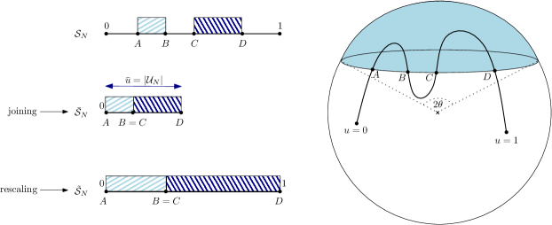
Figure 3: Illustration of the mechanism of the spherical cap bound.

only part of the locus, created by the signals in ${\cal S}_{N}$, is contained in a given spherical cap of angle $2\theta$. If we focus only on the subset of parameters values pertaining to signals within the spherical cap, and join these subsets to the left (see Fig. 3), we get a new system $\overline{{\cal S}}_{N}$ which modulates parameters in $[0,\overline{u})$ for some $\overline{u}\leq 1$, and uses the signals within the spherical cap only. If we then rescale the interval $[0,\overline{u})$ back to $[0,1)$ (while still using only signals within the same spherical cap), we get a new system $\tilde{{\cal S}}_{N}$, for parameters in $[0,1)$. The MP$\alpha$Es of the various systems ${\cal S}_{N}$, $\overline{{\cal S}}_{N}$ and $\tilde{{\cal S}}_{N}$ obey a simple relationship, and thus any bound on the MP$\alpha$E of $\tilde{{\cal S}}_{N}$ implies a bound on the MP$\alpha$E of ${\cal S}_{N}$. Specifically, using the unlimited-bandwidth converse bound (20) on the MP$\alpha$E exponent of $\tilde{{\cal S}}_{N}$ (even though it is a band-limited system) leads to the spherical cap bound. A key point in the proof is a measuring argument similar to [23, pp. 293-294], which is used to prove the existence of a spherical cap which contains a significant portion of the signal set locus. Finally, as the angle $\theta$ of the spherical cap was arbitrary, it is optimized to obtain the tightest bound. The following theorem is then obtained.

Theorem 2 (Spherical cap bound).

The MP$\alpha$E exponent per unit bandwidth is upper bounded as

$$F_{\alpha}(\Gamma)\leq\begin{cases}\gamma_{\alpha}\Gamma,&\Gamma<\frac{\alpha}{\gamma_{\alpha}}\\ \alpha\left[\log\left(\frac{\gamma_{\alpha}\Gamma}{\alpha}\right)+1\right],&\Gamma\geq\frac{\alpha}{\gamma_{\alpha}}\end{cases}.$$ (31)

Next, we outline the derivation of the spectrum replication bound. The proof relies on the idea of superimposing a frequency position modulation over a system ${\cal S}_{T}$ for bandwidth $W$. Suppose that we have a system ${\cal S}_{T}$ whose signals are band-limited to $[0,W)$. Imagine that we duplicate its signal set by a simple frequency shifts, from the frequency band $[0,W)$ to all the frequency bands $[mW,(m+1)W)$ for $0\leq m\leq M-1$, where $M$ is integer, thus obtaining a new signal set for a system $\tilde{{\cal S}}_{T}$. Now, a specific signal in the new signal set is specified by two components of the parameter: (i) the frequency band index $m$, and (ii) the signal within the band, which is nothing but a frequency translation of a signal from ${\cal S}_{T}$. The spectrum of the signals of ${\cal S}_{T}$ and $\tilde{{\cal S}}_{T}$ is illustrated in Fig. 4.

Figure 4: The system ${\cal S}_{T}$ is band-limited to $W$, and uses a linear combination of the orthonormal basis $\{\phi_{n}(t)\}_{n=1}^{N}$ to modulate the parameter $u$, where, here $N=3$. The orthonormal basis $\{\phi_{n}(t)\}_{n=1}^{3}$ is duplicated, using a frequency translation to the bands $[W,2W)$ and $[2W,3W)$. The new system $\tilde{{\cal S}}_{T}$, shown here with $M=3$, modulates the parameter $v$ by first choosing a frequency band $m\in\{0,1,2\}$, and then modulates $\{\phi_{n}(t)\}_{n=mM+1}^{mM+N}$, just as ${\cal S}_{T}$ modulates $\{\phi_{n}(t)\}_{n=1}^{N}$.

Accordingly, we can construct a modulation-estimation system $\tilde{{\cal S}}_{T}$ which modulates both parameters.

Specifically, let the newly constructed system be denoted by $\tilde{{\cal S}}_{T}$. The parameter at the input of this system is first uniformly quantized to $M$ values, and then the quantization error, after a proper scaling to $[0,1)$, is used as an input to the original system ${\cal S}_{T}$. The signal chosen from ${\cal S}_{T}$ is then modulated to one of $M$ possible non-overlapping frequency bands according to the quantized value of the parameter, and then transmitted over the channel.

At the receiver, first the active frequency band is decoded using a non-coherent decoder, and the quantized part is estimated. Then, the signal is demodulated to baseband (assuming a correct decoding at the first stage), and the estimator of ${\cal S}_{T}$ is used to estimate the quantization error. Afterwards, an estimation of the parameter is obtained using both the decoded quantized value and the estimation of the quantization error.

Now, on the one hand, the MP$\alpha$E exponent of the new system $\tilde{{\cal S}}_{T}$ can be lower bounded by an expression which depends on the MP$\alpha$E exponent of ${\cal S}_{T}$, i.e., $F_{\alpha}(\Gamma)$, and the probability of correct modulation frequency decoding. On the other hand, the signals of $\tilde{{\cal S}}_{T}$ occupy the frequency band $[0,MW)$, and if $M\gg 1$, these signals have a much larger bandwidth than the original system. Thus, it is proper to upper bound the MP$\alpha$E exponent of the new system $\tilde{{\cal S}}_{T}$ by the unlimited-bandwidth bound (20). Using these relations, a bound on $F_{\alpha}(\Gamma)$ can be readily obtained.

To state the spectrum replication bound, we need the following definitions. For $\rho\in[0,1]$ define

$$\Phi(\rho,\Gamma)\triangleq\rho[\eta-1-\log\eta]+\eta+\Gamma+\log\left[\frac{\sqrt{4\eta\Gamma+1}+1}{2\eta}\right]-\sqrt{4\eta\Gamma+1},$$ (32)

where

$$\eta=\frac{\Gamma+\sqrt{\Gamma^{2}-4(\rho^{2}+1)(\rho+1)^{2}}}{2(\rho+1)^{2}},$$ (33)

and also define

$$\Lambda_{\alpha}(\Gamma)\triangleq\sup_{0<\rho\leq 1}\left\{\frac{\Phi(\rho,\Gamma)-\gamma_{\alpha}\Gamma}{\rho}\right\}.$$ (34)

Theorem 3 (Spectrum replication bound).

The MP$\alpha$E exponent per unit bandwidth is upper bounded as

$$F_{\alpha}(\Gamma)\leq\gamma_{\alpha}\Gamma-\left[\alpha\Lambda_{\alpha}(\Gamma)\right]_{+}$$ (35)

where $[t]_{+}\triangleq\max\{t,0\}$.

It is evident that both bounds of (31) and (35) are monotonically increasing with $\gamma_{\alpha}$. Thus, in the range where the true value of $\gamma_{\alpha}$ is not known ($0<\alpha<2$), any upper bound on $\gamma_{\alpha}$ can be used, in particular, the bound (20).

As we shall see in Section IV, all the three converse bounds mentioned above, as far as we know, are the best available, at least for some $\alpha$ and $\Gamma$. However, for the sake of potential future improvement of these bounds, it is insightful to point out also their weaknesses. As discussed in [20, p. 839, footnote 6], the weakness of the channel coding converse bound does not stem from the use of Chebyshev’s inequality, but from the fact that there is no apparent single estimator which minimizes $\mathbb{P}_{u}\left\{\left|\hat{u}(\mathbf{Y})-u\right|>e^{-NR}\right\}$, uniformly for all $R$. The spherical cap bound suffers from the fact that an unlimited-bandwidth bound is used as a converse bound within the cap. The spectrum replication bound has the weakness that it is based on analyzing a two-stage estimator, which first decodes the frequency band, and then uses the signal in this band to estimate the parameter. Furthermore, in the first step, the frequency band is decoded using a sub-optimal, non-coherent decoder. Nonetheless, the above weaknesses are the result of compromises made to make the analysis reasonably tractable, and, as said, give non-trivial results.

We conclude this section with an achievability bound. The idea is to use a separation-based scheme, which first uniformly quantizes the parameter to $\exp(NR)$ points, for some $R>0$. Then, it maps the quantized parameter to a codeword from an ordinary channel code, which achieves the reliability function, $E(R,\Gamma)$. At the receiver, the maximum likelihood channel decoder is used to decode the transmitted codeword, and the estimated parameter is defined as the midpoint of the quantization interval of the decoded codeword. Note that increasing the rate $R$, reduces the quantization error, but increases the probability of decoding error and vice-versa. Thus, the rate is optimized in order to maximize the MP$\alpha$E exponent.

The derivation of this bound is a straightforward extension of [20]. We denote by $E(R,\Gamma)$ the reliability function of the AWGN channel (11) with SNR $\Gamma$, i.e., the maximal achievable error exponent for sequence of codes of rate $R$. As is well known, it can be assumed that the reliability function is for the maximal error probability over all codewords. We will use the definitions in (23) and (25).

Proposition 4 (Achievability bound).

The MP$\alpha$E exponent per unit bandwidth is lower bounded as

$$F_{\alpha}(\Gamma) \geq 2\cdot\max_{R\geq 0}\min\left\{E(R,\Gamma),\alpha R\right\}$$ (36)

$$\geq 2\cdot\max\left\{\sup_{0\leq\rho\leq 1}\frac{\alpha E_{0}(\rho,\Gamma)}{\rho+\alpha},\sup_{\rho\geq 1}\frac{\alpha E_{\mathrm{\scriptsize x}}(\rho,\Gamma)}{\rho+\alpha}\right\}.$$ (37)

Remark 5.

An achievable bound for the unlimited-bandwidth AWGN channel can be proved similarly to Proposition 4. In this case, the reliability function $E(R,\Gamma)$ in (36) is known exactly for all rates. With a slight change of arguments, it is given by [26]

$$E(R,C)=\begin{cases}\frac{C}{2}-R,&0\leq R\leq\frac{C}{4}\\ (\sqrt{C}-\sqrt{R})^{2},&\frac{C}{4}\leq R\leq C\end{cases},$$ (38)

where $C=\frac{P}{N_{0}}$. Since $\alpha R$ ($E(R,C)$) is an increasing (respectively, decreasing) function of $R$, when $\alpha\geq 2$, the solution of $2\cdot\max_{R\geq 0}\min\left\{E(R,C),\alpha R\right\}$ is obtained at $R=\frac{C}{2(\alpha+1)}=\frac{1}{2(\alpha+1)}\cdot\frac{P}{N_{0}}$. This proves the tightness of (20) for $\alpha\geq 2$.

Remark 6.

It was shown in [20] that this bound is tight in the extreme cases of $\alpha\to 0$ and $\alpha\to\infty$. This is indeed plausible since when $\alpha\to 0$ the error $|\hat{u}-u|^{\alpha}$ behaves like a “zero-one” loss function, in the sense that large errors do not incur more penalty than small errors. Thus, in this case, the quantization error dominates the MP$\alpha$E, and the rate is maximized, i.e. chosen to be the channel capacity. A similar situation occurs when $\alpha\to\infty$, but that in this case, the error $|\hat{u}-u|^{\alpha}$ tends to be a “zero-infinity” loss function. Large errors still do not penalize more than small errors, but any error event causes a catastrophically large penalty. Thus, in this case, the decoding error dominates the MP$\alpha$E, and the rate is minimized in order to maximize the decoding reliability, i.e. chosen to be zero. It should be stressed, however, that the achievability and converse bound are tight for a given $\Gamma$, as $\alpha\to 0$ and $\alpha\to\infty$, but may not be the best bounds for a given $0<\alpha<\infty$.

An apparent weakness of the achievability bound is that it is derived from analyzing a separation-based system, which means that the mapping between one of the $M$ possible quantized parameter values and the $M$ signal is arbitrary. A better system should choose this mapping such that nearby (quantized) parameter values will be mapped to nearby signals. In this case, a decoding error will typically cause only a small error in the parameter value. In other words, if one maps the quantized parameter value into bits, an unequal error protection scheme should be used to communicate these bits [27], with larger reliability for the most significant bits than for the least significant bits.

Typically, such a scheme uses an hierarchical channel code (also called superposition coding) [28], just like the one used, e.g., for the broadcast channel [29, Chapter 5]. Each codeword, in this case, is given by the sum of a ‘cloud’ codeword and a ‘satellite’ codeword, where the most significant bits determine the cloud codeword, and the least significant bits determine the satellite codeword. The advantage of such a system is that pairs of signals pertaining to nearby parameter values belong to the same ‘cloud’, whereas pairs of signals that are associated with distant parameter values are allowed to belong to different clouds. Thus, when a satellite decoding error occurs, this results in only an error in the refined part of the quantized parameter. Since the cloud centers have a rate lower than the entire codebook, the decoding error probability of the cloud centers can be significantly reduced, and overall, lead to a better MP$\alpha$E exponent. It can also be noticed that a scheme in the same spirit was used in the spectrum replication bound (Theorem 3), as a method to prove a converse bound on the exponent.

Unfortunately, despite a considerable effort in this direction, we were not able to find a concrete bound which improves the achievability bound. It seems that the problem is that strong bounds on the MP$\alpha$E can be obtained only by analyzing the optimal cloud decoder (as, e.g., in [30]), and not a decoder which treats the interference from the satellite as noise (as, e.g., in [31]). Especially, it seems that expurgated bounds for optimal cloud decoding are most useful for the problem of bounding the MP$\alpha$E. However, the best expurgated bound we are aware of was not sufficiently strong to improve the achievability bound on the MP$\alpha$E.

IV Results and Comparison among the Bounds

In Figures 5-8, the values $\alpha=0.1,1,2,10$ are considered, and the channel coding converse bound (28), the spherical cap bound (31), and the spectrum replication bound (35) are plotted (using (20) to bound $\gamma_{\alpha}$). For the sake of comparison, the unlimited-bandwidth converse bound (20), and the achievability bound (37) are also plotted.

It is evident that for $\alpha=0.1$, the channel coding converse bound dominates all other bounds; for $\alpha=1$ the spherical cap bound is better for some values of $\Gamma$, but for most SNRs the channel coding converse bound is the best; for $\alpha=2$ the spherical cap bound is best for some values of $\Gamma$, but for most SNRs the spectrum replication bound is the best; and, for $\alpha=10$ the spherical cap bound dominates all other bounds.

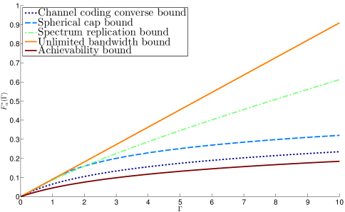
Figure 5: Various bounds on $F_{\alpha}(\Gamma)$ for $\alpha=0.1$.

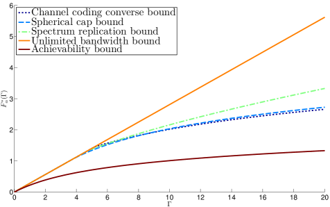
Figure 6: Various bounds on $F_{\alpha}(\Gamma)$ for $\alpha=1$.

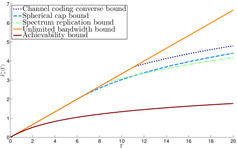
Figure 7: Various bounds on $F_{\alpha}^{*}(\Gamma)$ for $\alpha=2$.

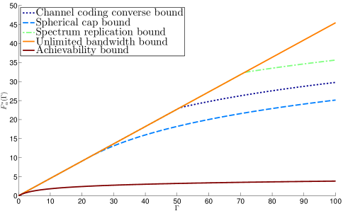
Figure 8: Various bounds on $F_{\alpha}(\Gamma)$ for $\alpha=10$.

To investigate systematically the behavior of the bounds for different values of $\alpha$, we explore the high and low SNR regimes. At high SNR, $\Gamma\to\infty$, it turns out that the all the converse bounds have the same asymptotic form $\alpha\log(\Gamma)+c_{\alpha}+o(\Gamma)$, for some $c_{\alpha}$. Thus, the various upper bounds differ by their additive constant $c_{\alpha}$. The next proposition gives the value of the constant $c_{\alpha}$. Its proof, as well as the proofs of all the other propositions in this section can be found in Appendix C.

Proposition 7.

The converse bounds at $\Gamma\to\infty$ are given by

$$F_{\alpha}(\Gamma)\leq\alpha\log(\Gamma)+c_{\alpha}+o(\Gamma)$$ (39)

with

$$c_{\alpha}=\begin{cases}\alpha-(1+\alpha)\log(1+\alpha),&\mbox{Channel coding converse bound (Prop. \ref{prop:Channel coding upper bound})}\\ \alpha\log\left(\frac{\gamma_{\alpha}}{\alpha}\right)+\alpha,&\mbox{Spherical cap bound (Thm. \ref{thm:Spherical cap bound})}\\ \alpha\log\left(\frac{e}{8}\right),&\mbox{Spectrum replication bound (Thm. \ref{thm: spectrum replication bound} ), }\alpha\geq 2.\end{cases}$$ (40)

For $\alpha<2$ the spectrum replication bound of Theorem 3 increases linearly with $\Gamma$, and is thus useless for high SNR.

Fig. 9 shows the value of $c_{\alpha}$ versus $\alpha$. As can be seen, for $0<\alpha\leq 1.34$, the channel coding converse bound has the best constant, for $1.34<\alpha\leq 2$ and $\alpha\geq 3$, the spherical cap bound has the best constant, and for $2<\alpha\leq 3$, the spectrum replication bound has the best constant. Nonetheless, if the bound (20) is not really tight for $\alpha<2$, and its actual value is $\gamma_{\alpha}=\frac{\alpha}{2(1+\alpha)}$, just as for $\alpha\geq 2$, then the spectrum replication bound would be the best for all $\alpha\leq 3$ (see Remark 12).

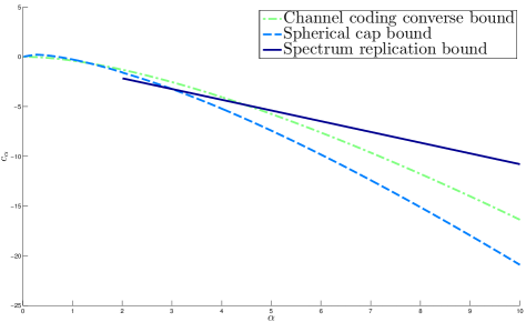
Figure 9: $c_{\alpha}$ for the various bounds, when using (20) as an upper bound to $\gamma_{\alpha}$.

We remark that the DPT based bound (5), given by

$$F_{\alpha}(\Gamma)\leq\alpha\cdot\log(1+\Gamma),$$ (41)

is not displayed in Figures 5-8, since it is worse than the best all other converse bounds. For high SNR, this is also evident from Fig. 9, by noting that $c_{\alpha}<0$ if we take the minimum over of all bounds (cf. (39) and (41)). Regarding the achievability bound of Proposition 4, a slightly weaker statement can be made.

Proposition 8.

The achievability bound of Prop. 4 scales as $[1+o(\Gamma)]\cdot\alpha\log(\Gamma)$ as $\Gamma\to\infty$.

At the other extreme, at low SNR ($\Gamma\to 0$), it is apparent that just like in channel coding, the bandwidth constraint is immaterial, and the performance of band-limited systems approaches that of unlimited-bandwidth systems. In this regime, the additional dimensions offered by a possible increase of the bandwidth do not improve the exponent, because the increase in the MP$\alpha$E exponent due to the additional dimensions is lower than the decrease in the exponent due to energy reduction in the original dimensions. Proposition 9 describes the behavior of the channel coding converse bound for small $\Gamma$.

Proposition 9.

The channel coding converse bound of Prop. 4 scales as $\frac{\alpha}{2(1+\alpha)}\Gamma+\Theta(\Gamma^{2})$ as $\Gamma\to 0$.

For $\alpha\geq 2$ the channel coding converse bound is linear in $\Gamma$, and has the same slope as the unlimited-bandwidth converse bound $\gamma_{\alpha}\Gamma$ (see (20)). For $\alpha<2$, however, there is still a gap.

Nevertheless, as the SNR increases, the band-limited exponent should be strictly less than the unlimited-bandwidth exponent. From this aspect, an interesting figure merit for a bound is the minimal SNR for which the bound deviates from the unlimited-bandwidth bound. For the spherical cap bound, this SNR is clearly $\Gamma_{\mathrm{\scriptsize sc}}\triangleq\frac{\alpha}{\gamma_{\alpha}}$. For the channel coding converse bound, such an SNR $\Gamma_{\mathrm{\scriptsize cc}}$ exists, but it is difficult to find it analytically. Indeed, as $\Gamma\to 0$, we get $\beta_{0}\to 1$ and the channel coding converse bound reads

$$F_{\alpha}(\Gamma)\leq\frac{\alpha}{1+\alpha}\Gamma+\Theta(\Gamma^{2}),$$ (42)

and as evident from (20), the minimization in (28) is dominated by the term $\gamma_{\alpha}\Gamma$. For the spectrum replication bound, the minimal SNR $\Gamma_{\mathrm{\scriptsize sp}}$ for which the bound deviates from the unlimited-bandwidth bound is also difficult to find analytically. Thus, numerical results are displayed in Fig. 10. From this aspect, it is seen that the spherical cap bound is usually better than the two other bounds, except for very low values of $\alpha$.

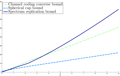
Figure 10: The minimal SNR for which a band-limited bound deviates from the unlimited-bandwidth bound, as a function of $\alpha$.

It is also interesting to note that for a given $\Gamma$, all bounds tend to zero as $\alpha\to 0$. For $\alpha\to\infty$ the spectrum replication bound is useless, whereas the channel coding and spherical cap bounds tend to $\frac{\Gamma}{2}$; the latter being the channel capacity of the unlimited-bandwidth channel (per unit time per unit bandwidth).

Appendix A Proofs of Converse Bounds

Proof:

As said in Section II, any band-limited signal $s(t,u)$ of energy $PT$ can be identified with a vector $\mathbf{s}(u)\triangleq(s_{1}(u),\ldots s_{N}(u))\in\mathbb{R}^{N}$, where $N=2WT$ (see (8)). Due to the power constraint, $\mathbf{s}(u)$ lies on the surface of the of radius $\sqrt{PT}$, centered at the origin.

We begin with a few definitions. With some abuse of notation, the system ${\cal S}_{N}$ will be identified with the projection vectors of the signals in ${\cal S}_{T}$, i.e., ${\cal S}_{N}\triangleq\left\{\mathbf{s}(u):\;u\in[0,1)\right\}$, and its MP$\alpha$E will be denoted by $e_{\alpha}({\cal S}_{N})$, where the estimator will be understood from context. We denote the set of parameters values pertaining to a signal subset $\overline{{\cal S}}_{N}\subseteq{\cal S}_{N}$, by $\mathbb{U}(\overline{{\cal S}}_{N})$, i.e., $u\in\mathbb{U}(\overline{{\cal S}}_{N})$ iff $\mathbf{s}(u)\in\overline{{\cal S}}_{N}$. Also, we denote by $\left|\mathbb{U}(\overline{{\cal S}}_{N})\right|$ the standard Lebesgue measure of the set $\mathbb{U}(\overline{{\cal S}}_{N})\subseteq[0,1)$. Furthermore, for any unit vector $\mathbf{g}\in\mathbb{R}^{N}$ and an angle $\theta\in[0,\pi]$ we define the spherical cap as

$${\cal A}_{\theta}(\mathbf{g},{\cal S}_{N})\triangleq\left\{\mathbf{s}(u)\in{\cal S}_{N}:\;\left\langle\mathbf{s}(u),\mathbf{g}\right\rangle\geq\sqrt{PT}\cdot\cos\theta\right\},$$ (A.1)

where, as usual, the inner product is defined as $\left\langle\mathbf{s}(u),\mathbf{g}\right\rangle\triangleq\sum_{n=1}^{N}s_{n}(u)\cdot g_{n}$. We begin with the following measuring argument.

Lemma 10.

Let $\theta\in(0,\frac{\pi}{2})$ and ${\cal S}_{N}$ be given. Then, there exists unit vector $\mathbf{g}$ for which

$$\left|{\cal\mathbb{U}}\left[{\cal A}_{\theta}(\mathbf{g},{\cal S}_{N})\right]\right|\geq\exp\left\{\frac{N}{2}\cdot\left[\log\left(\sin^{2}\theta\right)-\Theta\left(\frac{\log N}{N}\right)\right]\right\}.$$ (A.2)

Proof:

The idea of the proof is similar to [23, pp. 293-294]. Let $A_{N}(\theta)$ denote the surface area of a spherical cap of angle $\theta$ on a sphere of radius $\sqrt{PT}$, in an $N$ dimensional space. Note that $A_{N}(\pi)$ is the surface area of the entire sphere. Now, define

$$\Xi\triangleq\int_{0}^{1}\int_{{\cal B}_{N}}\mathbb{I}\left\{\left\langle\mathbf{s}(u),\mathbf{g}\right\rangle\geq S\cdot\cos\theta\right\}\mathrm{d}{\cal B}_{N}(\mathbf{g})\cdot\mathrm{d}u$$ (A.3)

where ${\cal B}_{N}$ is the surface of the $N$-dimensional unit sphere and $\mathrm{d}{\cal B}_{N}(\mathbf{g})$ is a differential surface area around $\mathbf{g}$. On the one hand, $\Xi$ is trivially given by $A_{N}(\theta)$. On the other hand, using Fubini’s theorem [32, Chapter 18], $\Xi$ can also be expressed with the integration order exchanged, and so

$$\Xi =\int_{{\cal B}_{N}}\int_{0}^{1}\mathbb{I}\left\{\left\langle\mathbf{s}(u),\mathbf{g}\right\rangle\geq S\cdot\cos\theta\right\}\mathrm{d}u\cdot\mathrm{d}{\cal B}_{N}(\mathbf{g})$$ (A.4)

$$=\int_{{\cal B}_{N}}\left|\mathbb{U}\left[{\cal A}_{\theta}(\mathbf{g},{\cal S}_{N})\right]\right|\mathrm{d}{\cal B}_{N}(\mathbf{g})$$ (A.5)

$$\leq A_{N}(\pi)\cdot\max_{\mathbf{g}\in{\cal B}_{N}}\left|{\cal\mathbb{U}}\left[{\cal A}_{\theta}(\mathbf{g},{\cal S}_{N})\right]\right|.$$ (A.6)

Thus, there exists $\mathbf{g}\in{\cal B}_{N}$ such that

$$\left|\mathbb{U}\left[{\cal A}_{\theta}(\mathbf{g},{\cal S}_{N})\right]\right|\geq\frac{A_{N}(\theta)}{A_{N}(\pi)}.$$ (A.7)

To conclude, we use [33, eqs. (27) and (28)]

$$\frac{A_{N}(\theta)}{A_{N}(\pi)}=\frac{\exp\left[N\log\left(\sin\theta\right)\right]}{\sqrt{2\pi N}\cdot\sin\theta\cdot\cos\theta}\cdot\left[1+O\left(\frac{1}{N}\right)\right]=\exp\left\{\frac{N}{2}\left[\log\left(\sin^{2}\theta\right)-\frac{\log(N)}{N}-\frac{O(1)}{N}\right]\right\}.$$ (A.8)

∎

Let ${\cal S}_{N}$ be given, and denote its estimator by $\hat{u}(\mathbf{y})$. In addition, let $\mathbf{g}$ be a unit vector that satisfies (A.2), and let ${\cal U}_{N}\triangleq\mathbb{U}\left[{\cal A}_{\theta}(\mathbf{g},{\cal S}_{N})\right]$ the corresponding parameter values of its spherical cap. We shall now construct from ${\cal S}_{N}$, two modulation-estimation systems, ${\cal\overline{S}}_{N}$ and $\tilde{{\cal S}}_{N}$, using signals only from ${\cal A}_{\theta}(\mathbf{g},{\cal S}_{N})$, such that

$$e_{\alpha}({\cal S}_{N})\geq e_{\alpha}(\overline{{\cal S}}_{N})\geq\left|{\cal U}_{N}\right|^{\alpha}\cdot e_{\alpha}(\tilde{{\cal S}}_{N}).$$ (A.9)

Now, although $\tilde{{\cal S}}_{N}$ is band-limited just like ${\cal S}_{N}$, we will bound $e_{\alpha}(\tilde{{\cal S}}_{N})$ using the unlimited-bandwidth bound. This and (A.9) will provide a bound on $F_{\alpha}(\Gamma)$.

To construct $\overline{{\cal S}}_{N}$, we shall map ${\cal U}_{N}$ onto $\overline{{\cal U}}_{N}\triangleq[0,|{\cal U}_{N}|)$ in an order preserving manner (see Fig. 3). For example, if ${\cal U}_{N}=\bigcup_{i=1}^{I}{\cal I}_{i}$, where ${\cal I}_{i}$ are disjoint intervals of the form $[a_{i},b_{i})$, and $a_{1}<b_{1}\leq a_{2}<\cdots<a_{I}\leq b_{I}$ then such a mapping is easily obtained by eliminating the spaces between every two consecutive intervals. Indeed, at the first step, the interval ${\cal I}_{I}$ will be shifted by $a_{I}-b_{I-1}$ to the left, such that ${\cal I}_{I-1}$ and ${\cal I}_{I}$ are combined into a single interval ${\cal I}_{I-1}^{(1)}$, while ${\cal I}_{i}^{(1)}={\cal I}_{i}$ is set for $1\leq i<I-1$. At the second step, the interval ${\cal I}_{I-1}^{(1)}$ is combined with ${\cal I}_{I-2}^{(1)}$ to a single interval ${\cal I}_{I-2}^{(2)}$ in the same manner. Continuing in this manner for $I-1$ steps, we obtain a single interval, which can be translated to $[0,|{\cal U}_{N}|)$. More generally, it is easy to verify that the mapping

$$\Psi[u]\triangleq\int_{0}^{u}\mathbb{I}\left[w\in{\cal U}_{N}\right]\mathrm{d}w$$ (A.10)

satisfies the required properties. Note that the integral in (A.10) exists since the mapping $u\to s(t,u)$ is assumed to be measurable. The function $\Psi[\cdot]$ is monotonic and Lipschitz continuous with constant $1$ as

$$\left|u_{1}-u_{2}\right|\geq\left|\Psi[u_{1}]-\Psi[u_{2}]\right|$$ (A.11)

for any $u_{1},u_{2}\in[0,1)$. So, using the estimator $\overline{u}(\mathbf{y})\triangleq\Psi[\hat{u}(\mathbf{y})]$ for $\overline{{\cal S}}_{N}$, we have

$$\mathbb{E}_{u}\left\{\left|\hat{u}(\mathbf{Y})-u\right|^{\alpha}\right\}\geq\mathbb{E}_{\Psi[u]}\left\{\left|\Psi[\hat{u}(\mathbf{Y})]-\Psi[u]\right|^{\alpha}\right\},$$ (A.12)

for any $u\in{\cal U}_{N}$, where in the left-hand side (right-hand side) the system ${\cal S}_{N}$ (respectively, $\overline{{\cal S}}_{N}$) is assumed. Hence,

$$e_{\alpha}({\cal S}_{N})\geq e_{\alpha}(\overline{{\cal S}}_{N}).$$ (A.13)

Now, consider the signal set

$${\cal\tilde{S}}_{N}\triangleq\left\{\tilde{\mathbf{s}}(u)=\mathbf{s}(u)-\left\langle\mathbf{s}(u),\mathbf{g}\right\rangle\cdot\mathbf{g}:\;\mathbf{s}(u)\in{\cal A}_{\theta}(\mathbf{g},{\cal S}_{N})\right\}.$$ (A.14)

To wit, geometrically, this is the signal set obtained by removing the projecting of the signal vector $\mathbf{s}(u)$ onto $\mathbf{g}$ from $\mathbf{s}(u)$. Clearly, for any $\mathbf{s}(u)\in{\cal A}_{\theta}(\mathbf{g},{\cal S}_{N})$ and it corresponding $\tilde{\mathbf{s}}(u)\in\tilde{{\cal S}}_{N}$ according to (A.14),

$$PT =\left\|\mathbf{s}(u)\right\|^{2}$$ (A.15)

$$=\left\|\mathbf{s}(u)-\left\langle\mathbf{s}(u),\mathbf{g}\right\rangle\cdot\mathbf{g}+\left\langle\mathbf{s}(u),\mathbf{g}\right\rangle\cdot\mathbf{g}\right\|^{2}$$ (A.16)

$$\overset{{\scriptstyle(a)}}{=}\left\|\tilde{\mathbf{s}}(u)\right\|^{2}+\left\|\left\langle\mathbf{s}(u),\mathbf{g}\right\rangle\cdot\mathbf{g}\right\|^{2}$$ (A.17)

$$\geq\left\|\tilde{\mathbf{s}}(u)\right\|^{2}+PT\cdot\cos^{2}\theta,$$ (A.18)

where $(a)$ follows from the Pythagorean theorem and the orthogonality of $\tilde{\mathbf{s}}(u)$ and $\mathbf{g}$. Thus, the signal set $\tilde{{\cal S}}_{N}$ satisfies an energy constraint of $PT[1-\cos^{2}\theta]=PT\cdot\sin^{2}\theta$.

We can now construct a modulation-estimation system which is based on the signal set $\tilde{{\cal S}}_{N}$ and the original domain of the parameter. This is simply done by scaling back $\overline{{\cal U}}_{N}=[0,|{\cal U}_{N}|)$ to the original interval $[0,1)=|{\cal U}_{N}|^{-1}\cdot[0,|{\cal U}_{N}|)$. The system operates as follows. To modulate a parameter $v\in[0,1)$, first $u(v)$ is set to

$$u(v)=\Psi^{-1}\left[|{\cal U}_{N}|^{-1}\cdot v\right],$$ (A.19)

i.e. the parameter $v\in[0,1)$ is first mapped to $\overline{{\cal U}}_{N}$ and then mapped to the $u\in[0,1)$ that satisfies $\mathbf{s}\left(u(v)\right)\in{\cal A}_{\theta}(\mathbf{g},{\cal S}_{N})$. Then, $s\left(t,u(v)\right)=\sum s_{n}\left(u(v)\right)\cdot\phi_{n}(t)$ is transmitted over the channel (6). The estimator $\hat{v}(\mathbf{y})$ of $v$, is given by

$$\hat{v}(\mathbf{y})=|{\cal U}_{N}|^{-1}\cdot\overline{u}(\mathbf{y}).$$ (A.20)

Now, due to the scaling operation from $\overline{{\cal S}}_{N}$ to $\tilde{{\cal S}}_{N}$ by a factor of $|{\cal U}_{N}|^{-1}$, the ratio between their MP$\alpha$E’s is not larger than $|{\cal U}_{N}|^{-\alpha}$, to wit, for any given $v\in[0,1)$

$$\mathbb{E}_{v}\left\{\left|\hat{v}(\mathbf{Y})-v\right|^{\alpha}\right\}\leq|{\cal U}_{N}|^{-\alpha}\cdot\mathbb{E}_{|{\cal U}_{N}|\cdot v}\left\{\left|\overline{u}(\mathbf{y})-|{\cal U}_{N}|\cdot v\right|^{\alpha}\right\}$$ (A.21)

where in the left-hand side (right-hand side) the system $\tilde{{\cal S}}_{N}$ (respectively, $\overline{{\cal S}}_{N}$) is assumed. This, together with (A.13) implies (A.9).

Now, we note that the modulation-estimation system for $v$ has a power limitation of $PT\cdot\sin^{2}\theta$. So, a lower bound for the MP$\alpha$E of unlimited-bandwidth systems can be used to obtain to lower bound the left-hand side of (A.21), and hence,

$$\mathbb{E}_{v}\left\{\left|\hat{v}(\mathbf{Y})-v\right|^{\alpha}\right\}\geq\exp\left[-\frac{N}{2}\gamma_{\alpha}\Gamma\sin^{2}\theta\right].$$ (A.22)

This, along with (A.9) and Lemma 10, implies that for any given $\delta>0$, there exists $N$ sufficiently large such that

$$\mathbb{E}_{u}\left\{\left|\hat{u}(\mathbf{Y})-u\right|^{\alpha}\right\}\geq\exp\left\{\frac{N}{2}\cdot\alpha\left[\log\left(\sin^{2}\theta\right)-\delta\right]\right\}\exp\left[-\frac{N}{2}\gamma_{\alpha}\Gamma\sin^{2}\theta\right].$$ (A.23)

Now, the angle $\theta\in(0,\frac{\pi}{2})$ is arbitrary, and thus can be optimized. Denoting $\tau\triangleq\sin^{2}\theta$ we get

$$\mathbb{E}_{u}\left\{\left|\hat{u}(\mathbf{Y})-u\right|^{\alpha}\right\}\geq\exp\left\{-\frac{N}{2}\left[\sup_{0<\tau<1}\left(\gamma_{\alpha}\Gamma\tau-\alpha\log\tau\right)-\alpha\delta\right]\right\},$$ (A.24)

and after maximizing over $\tau$, and taking $\delta\downarrow 0$, (31) is immediately obtained. ∎

Proof:

Let $\delta>0$ be given. As in the proof of the spherical cap bound, let a signal set ${\cal S}_{N}\triangleq\left\{\mathbf{s}(u):\;u\in[0,1)\right\}$ be given. As was discussed in Section II, for any given dimension, we can transform a vector $\mathbf{s}(u)$ to a signal $s(t,u)$ using an orthonormal basis $\{\phi_{n}(t)\}$. Specifically, let us consider an orthonormal basis of $L\triangleq MN$ signals $\{\phi_{l}(t),\;0\leq t\leq T\}_{l=1}^{L}$, where $M\gg 1$, and $M$ integer. We assume that the system ${\cal S}_{N}$ uses $\{\phi_{l}(t),\;0\leq t\leq T\}_{l=1}^{N}$ to transform $\mathbf{s}(u)\in\mathbb{R}^{N}$ to a signal $s(t,u)$. We now construct a new system, that modulates a parameter $v\in[0,1)$, using a signal set $\tilde{{\cal S}}_{N}\in\mathbb{R}^{L}$ , which is transformed to a signal using $\{\phi_{l}(t),\;0\leq t\leq T\}_{l=1}^{L}$. Since $N=2WT$ and $L=2MWT$, as said in Section III, one can think of the system $\tilde{{\cal S}}_{N}$ as using bandwidth $MW\gg W$. Its total frequency band $[0,MW)$ is partitioned into $M$ consecutive frequency bands $[0,W)$, $[W,2W)$,…, $[(M-1)W,MW)$, and the value of the parameter is modulated using both the choice of active frequency band $0\leq m\leq M-1$, and the specific signal within the band.

We now describe the system $\tilde{{\cal S}}_{N}$ which modulates $v\in[0,1)$. Let $v_{\mathrm{\scriptsize c}}=\frac{\left\lfloor M\cdot v\right\rfloor}{M}$, where $\left\lfloor\cdot\right\rfloor$ is the floor operation, and $v_{\mathrm{\scriptsize r}}=v-v_{\mathrm{\scriptsize c}}$. The idea is to use $v_{\mathrm{\scriptsize c}}$ to choose one of $M$ possible sets of basis functions $\left\{\{\phi_{l}\}_{l=1}^{N},\{\phi_{l}\}_{l=N+1}^{2N},\ldots\{\phi_{l}\}_{l=(M-1)N+1}^{MN}\right\}$, and to use $v_{\mathrm{\scriptsize r}}$ to choose which vector to transmit over the chosen $N$ basis functions, while utilizing the original system ${\cal S}_{N}$.

The modulation-estimation system $\tilde{{\cal S}}_{N}$ is depicted in Fig. 11 (in continuous time).

Figure 11: Modulation-Estimation system for the proof of the spectrum replication bound.

Specifically, to modulate $v$, a modulation index is chosen using the coarse part as

$$m(v)\triangleq M\cdot v_{\mathrm{\scriptsize c}}\in\{0,\ldots,M-1\},$$ (A.25)

and a vector of coefficients is chosen as $\mathbf{s}(M\cdot v_{\mathrm{\scriptsize r}})$. Then, $\tilde{\mathbf{s}}(v)$, the coefficient vector of $\tilde{{\cal S}}_{N}$, is chosen with the entries

$$\tilde{s}_{l}(v)=\begin{cases}s_{l-m(v)}(M\cdot v_{\mathrm{\scriptsize r}}),&m(v)N+1\leq l\leq m(v)N+N\\ 0,&\mbox{otherwise}\end{cases}$$ (A.26)

(note that $M\cdot v_{\mathrm{\scriptsize r}}\in[0,1)$), and $\tilde{s}(t,v)=\sum_{l=1}^{L}\tilde{s}_{l}(v)\cdot\phi_{l}(t)$ is transmitted over the channel (6). To wit, only the signals $\{\phi_{l}(t)\}_{l=m(v)N+1}^{m(v)N+N}$, which represent the frequency band $[m(v)W,(m(v)+1)W)$, have non-zero coefficients.

At the receiver, a proper projection vector $\tilde{\mathbf{y}}$ is obtained as in (9), but this time, over $L$ basis functions. Specifically, we define the projections

$$\tilde{y}_{m,n}\triangleq\int_{0}^{T}y(t)\cdot\tilde{\phi}_{mN+n}(t)\cdot\mathrm{d}t\quad 0\leq m\leq M-1,\quad 1\leq n\leq N,$$ (A.27)

and $\tilde{\mathbf{y}}_{m}\triangleq(\tilde{y}_{m,1},\ldots,\tilde{y}_{m,N})$, as well as the (scaled) energies $q_{m}\triangleq\frac{2}{N_{0}}\left\|\tilde{\mathbf{y}}_{m}\right\|^{2}=\frac{2}{N_{0}}\sum_{n=1}^{N}\tilde{y}_{m,n}^{2}.$ The estimator $\hat{v}(\tilde{\mathbf{y}})$ of $\tilde{{\cal S}}_{N}$ is obtained in two steps. In the first, we decode $m(v)$, using a non-coherent decoder, which decides based on the maximum projection energy, i.e.

$$\hat{m}(\tilde{\mathbf{y}})\triangleq\operatorname*{arg\,max}_{m\in\{0,\ldots,M-1\}}q_{m}.$$ (A.28)

In the second step, we estimate the parameter $v$ as

$$\hat{v}(\tilde{\mathbf{y}})=\frac{\hat{m}+\hat{u}(\tilde{\mathbf{y}}_{\hat{m}})}{M},$$ (A.29)

where $\hat{u}(\mathbf{y})$ is the estimator of the original system ${\cal S}_{N}$, and for clarity, the dependence of $\hat{m}$ on $\tilde{\mathbf{y}}$ was omitted. In words, in the second step, we assume that $\hat{m}$ is the correct index, and use the vector $\tilde{\mathbf{y}}_{\hat{m}}$ as the input to the estimator of ${\cal S}_{N}$.

The exponential behavior of the MP$\alpha$E of the system $\tilde{{\cal S}}_{N}$ will be different from that of ${\cal S}_{N}$ only if $M$ increases exponentially with $N$. Hence, we assume that $M\triangleq\exp(TWR)=\exp(\frac{N}{2}\cdot R)$ for some ‘rate’ $R>0$. In Appendix B, we analyze the reliability of the non-coherent decoder, using large deviations analysis of chi-square random variables. Denoting the error event, in the first step of the estimation, by ${\cal E}$, it is shown there that for all $v\in[0,1)$

$$\mathbb{P}_{v}[{\cal E}]\leq\exp\left[-\frac{N}{2}\cdot G(\Gamma,R)\right]$$ (A.30)

where

$$G(\Gamma,R)\triangleq\max_{0\leq\rho\leq 1}\left\{\Phi(\rho,\Gamma)-\rho R\right\}$$ (A.31)

and $\Phi(\rho,\Gamma)$ is as defined in (32). The MP$\alpha$E of $\tilde{{\cal S}}_{N}$ is then bounded as follows. For all $N$ sufficiently large

$$\mathbb{E}_{v}\left\{\left|\hat{v}(\mathbf{\tilde{Y}})-v\right|^{\alpha}\right\} =\mathbb{P}_{v}[{\cal E}]\cdot\mathbb{E}_{v}\left\{\left|\hat{v}(\mathbf{\tilde{Y}})-v\right|^{\alpha}|{\cal E}\right\}+\mathbb{P}_{v}[{\cal E}^{c}]\cdot\mathbb{E}_{v}\left\{\left|\hat{v}(\mathbf{\tilde{Y}})-v\right|^{\alpha}|{\cal E}^{c}\right\}$$ (A.32)

$$\leq\mathbb{P}_{v}[{\cal E}]+\mathbb{E}_{v}\left\{\left|\hat{v}(\mathbf{\tilde{Y}})-v\right|^{\alpha}|{\cal E}^{c}\right\}$$ (A.33)

$$\leq\exp\left[-\frac{N}{2}\cdot G(\Gamma,R)\right]+\mathbb{E}_{v}\left\{\left|\hat{v}(\mathbf{\tilde{Y}})-v\right|^{\alpha}|{\cal E}^{c}\right\}$$ (A.34)

$$=\exp\left[-\frac{N}{2}\cdot G(\Gamma,R)\right]+\mathbb{E}_{v}\left\{\left.\left|\frac{\hat{m}(\tilde{\mathbf{Y}})}{M}+\frac{\hat{u}(\tilde{\mathbf{Y}}_{\hat{m}(\tilde{\mathbf{Y}})})}{M}-v_{\mathrm{\scriptsize c}}-v_{\mathrm{\scriptsize r}}\right|^{\alpha}\right|{\cal E}^{c}\right\}$$ (A.35)

$$\overset{{\scriptstyle(a)}}{\leq}\exp\left[-\frac{N}{2}\cdot G(\Gamma,R)\right]+2\cdot\mathbb{E}_{v}\left\{\left|\frac{\hat{u}(\tilde{\mathbf{Y}}_{m(v)})}{M}-v_{\mathrm{\scriptsize r}}\right|^{\alpha}\right\}$$ (A.36)

$$=\exp\left[-\frac{N}{2}\cdot G(\Gamma,R)\right]+\frac{2}{M^{\alpha}}\mathbb{E}_{u}\left\{\left|\hat{u}(\tilde{\mathbf{Y}}_{m(v)})-M\cdot u_{\mathrm{\scriptsize r}}\right|^{\alpha}\right\}$$ (A.37)

$$\leq\exp\left[-\frac{N}{2}\cdot G(\Gamma,R)\right]+2\cdot\exp\left\{-\frac{N}{2}\cdot\left[\alpha R+F_{\alpha}(\Gamma)\right]\right\}$$ (A.38)

$$\leq 2\cdot\exp\left\{-\frac{N}{2}\cdot\min\left[G(\Gamma,R),\alpha R+F_{\alpha}(\Gamma)\right]\right\}.$$ (A.39)

In $(a)$, we have used the fact that conditioned on ${\cal E}^{c}$, we have $\frac{\hat{u}(\tilde{\mathbf{Y}}_{\hat{m}})}{M}=v_{\mathrm{\scriptsize c}}$ and the fact that for $G(\Gamma,R)>0$ (which is our regime of interest), (A.30) implies that $\mathbb{P}_{v}[{\cal E}^{c}]\to 1$ as $N\to\infty$. So, for any random variable $X$, and all $N$ sufficiently large,

$$\mathbb{E}_{v}\left\{X|{\cal E}^{c}\right\} =\frac{1}{\mathbb{P}_{v}[{\cal E}^{c}]}\mathbb{E}_{v}\left\{X\cdot\mathbb{I}[X\in{\cal E}^{c}]\right\}$$ (A.40)

$$\leq\frac{1}{\mathbb{P}_{v}[{\cal E}^{c}]}\mathbb{E}_{v}[X]$$ (A.41)

$$\leq 2\cdot\mathbb{E}_{v}[X].$$ (A.42)

Clearly, for any given $R\geq 0$, the proposed system cannot achieve an MP$\alpha$E exponent better than the converse bound of the unlimited-bandwidth system, $\exp(-\frac{N}{2}\cdot\gamma_{\alpha}\Gamma)$. Hence,

$$\min\left\{G(\Gamma,R),\alpha R+F_{\alpha}(\Gamma)\right\}\leq\gamma_{\alpha}\Gamma,$$ (A.43)

or, equivalently

$$F_{\alpha}(\Gamma)\leq\begin{cases}\gamma_{\alpha}\Gamma-\alpha R,&G(\Gamma,R)>\gamma_{\alpha}\Gamma\\ \infty,&G(\Gamma,R)\leq\gamma_{\alpha}\Gamma\end{cases}.$$ (A.44)

The relation $G(\Gamma,R)>\gamma_{\alpha}\Gamma$ can be easily seen to be equivalent to $R<\Lambda_{\alpha}(\Gamma)$, where $\Lambda_{\alpha}(\Gamma)$ is defined in (34), and thus

$$F_{\alpha}(\Gamma)\leq\begin{cases}\gamma_{\alpha}\Gamma-\alpha R,&R\leq\Lambda_{\alpha}(\Gamma)\\ \infty,&R>\Lambda_{\alpha}(\Gamma)\end{cases}.$$ (A.45)

Since $R\geq 0$ is arbitrary, the tightest bound is obtained by choosing $R=\Lambda_{\alpha}(\Gamma)$ which leads to (35). ∎

Appendix B Reliability Analysis of the Modulation Scheme of the Spectrum Replication Bound

In this appendix, we evaluate the reliability of the non-coherent decoder (A.28). Let us denote the random variables of the system by uppercase letters, e.g. $Q_{m}$. Due to symmetry, it can be assumed w.l.o.g. that $m_{v}=0$. Then, it is straightforward to verify that for any given $m\neq 0$, we have $\tilde{Y}_{m,n}\sim{\cal N}(0,1)$ and $\{\tilde{Y}_{m,n}\}$ are independent. Consequently, $Q_{m}$ is a chi-square random variable of $N$ degrees of freedom. Similarly, for $m=0$, we have $\tilde{Y}_{0,n}\sim{\cal N}(\varsigma_{M\cdot v_{\mathrm{\scriptsize r}},n},1)$ i.e., $Q_{0}$ is a non-central chi-square random variable of $N$ degrees of freedom, and a non-centrality parameter $\lambda\triangleq\frac{1}{\nicefrac{{N_{0}}}{{2}}}\sum_{n=1}^{N}\varsigma_{M\cdot v_{\mathrm{\scriptsize r}},n}^{2}=\frac{2PT}{N_{0}}$. We build on the analysis in [12, Section 2.5, Section 2.12.2, Problem 2.14 and Problem 2.15]. Let $f_{0}(\cdot)$ be the probability density function of $Q_{0}$ given that $m_{v}=0$. Then, for any $0\leq\rho\leq 1$, the decoding error probability can be bounded as

$$\mathbb{P}_{v}[{\cal E}] =1-\mathbb{P}\left[Q_{0}>Q_{m},\;\forall m\neq 0|m_{v}=0\right]$$ (B.1)

$$=\int_{0}^{\infty}f_{0}(q)\left\{1-\left(\mathbb{P}[Q_{1}\leq q|m_{v}=0]\right)^{M-1}\right\}\cdot\mathrm{d}q$$ (B.2)

$$\leq M^{\rho}\int_{0}^{\infty}f_{0}(q)\mathbb{P}^{\rho}[Q_{1}>q|m_{v}=0]\cdot\mathrm{d}q$$ (B.3)

where the inequality is obtained from $1-(1-\alpha)^{M}\leq(M\alpha)^{\rho}$ (known as Gallager’s union bound [6, Lemma, p. 136]). Let $\{K_{N}\}_{N=1}^{\infty}$ and $\{\kappa_{N}\}_{N=1}^{\infty}$ be two positive sequences which satisfy $K_{N}\uparrow\infty$ and $\kappa_{N}\downarrow 0$ as $N\to\infty$. The appropriate choices for them will be discussed later on. For notational simplicity, let us assume that $\nicefrac{{K_{N}}}{{\kappa_{N}}}$ is integer, and temporarily omit the subscript $N$ in their notation. Then,

$$\mathbb{P}_{v}[{\cal E}] \leq M^{\rho}\int_{0}^{\infty}f_{0}(q)\cdot\mathbb{P}^{\rho}[Q_{1}>q|m_{v}=0]\cdot\mathrm{d}q$$ (B.4)

$$\leq M^{\rho}\sum_{l=0}^{\frac{K}{\kappa}-1}\int_{l\kappa N}^{(l+1)\kappa N}f_{0}(q)\cdot\mathbb{P}^{\rho}[Q_{1}>q|m_{v}=0]\cdot\mathrm{d}q+M^{\rho}\mathbb{P}\left(Q_{0}>KN|m_{v}=0\right)$$ (B.5)

$$\leq M^{\rho}\sum_{l=0}^{\frac{K}{\kappa}-1}\int_{l\kappa N}^{(l+1)\kappa N}f_{0}(q)\cdot\mathbb{P}^{\rho}[Q_{1}>l\kappa N|m_{v}=0]\cdot\mathrm{d}q+M^{\rho}\mathbb{P}\left(Q_{0}>KN|m_{v}=0\right)$$ (B.6)

$$=M^{\rho}\sum_{l=0}^{\frac{K}{\kappa}-1}\mathbb{P}^{\rho}[Q_{1}>l\kappa N|m_{v}=0]\cdot\mathbb{P}\left[l\kappa N\leq Q_{0}\leq(l+1)\kappa N|m_{v}=0\right]$$

$$\hphantom{=}+M^{\rho}\mathbb{P}\left[Q_{0}>KN|m_{v}=0\right]$$ (B.7)

$$\leq M^{\rho}\frac{K}{\kappa}\cdot\left\{\max_{0\leq l\leq\frac{K}{\kappa}-1}\mathbb{P}^{\rho}[Q_{1}>l\kappa N|m_{v}=0]\cdot\mathbb{P}\left[l\kappa N\leq Q_{0}\leq(l+1)\kappa N|m_{v}=0\right]\right.$$

$$\hphantom{=}\left.\vphantom{\max_{0\leq l\leq\frac{K}{\kappa}-1}}+\mathbb{P}\left[Q_{0}>KN|m_{v}=0\right]\right\},$$ (B.8)

where in the last inequality, we have used the assumption that $\frac{K}{\kappa}>1$ for sufficiently large $N$. In order to evaluate the exponential behavior of $\mathbb{P}_{v}[{\cal E}]$, it will be convenient to partition the maximization to a few intervals. In each interval, we upper bound the objective

$$\mathbb{P}^{\rho}[Q_{1}>l\kappa N|m_{v}=0]\cdot\mathbb{P}\left[l\kappa N\leq Q_{0}\leq(l+1)\kappa N|m_{v}=0\right]$$ (B.9)

by an asymptotically tight upper bound. In essence, we are replacing the probability of an interval by the tail probability of one of its endpoints, according to the relative position of $l\kappa N$ w.r.t. $\mathbb{E}[Q_{0}]=N$ and $\mathbb{E}[Q_{1}]=N+\lambda=N+\frac{2PT}{N_{0}}=N(1+\Gamma)$, see Fig. 12.

Figure 12: The probability distribution functions of $Q_{0}$ and $Q_{1}$, for $N=10$ and $\Gamma=2$.

Let $l_{1}$ be such that $l_{1}\kappa\leq 1\leq(l_{1}+1)\kappa$ and $l_{2}$ be such that $l_{2}\kappa\leq 1+\Gamma\leq(l_{2}+1)\kappa$. Then, for $l\leq l_{1}-1$ we upper bound (B.9) by

$$\mathbb{P}\left[Q_{0}\leq(l+1)\kappa N|m_{v}=0\right],$$ (B.10)

for $l_{1}\leq l\leq l_{2}-1$ we upper bound it by

$$\mathbb{P}^{\rho}[Q_{1}>l\kappa N|m_{v}=0]\cdot\mathbb{P}\left[Q_{0}\leq(l+1)\kappa N|m_{v}=0\right],$$ (B.11)

for $l=l_{2}$ we upper bound it by

$$\mathbb{P}^{\rho}[Q_{1}>l\kappa N|m_{v}=0],$$ (B.12)

and for $l_{2}+1\leq l\leq\frac{K}{\kappa}-1$ we upper bound it by

$$\mathbb{P}^{\rho}[Q_{1}>l\kappa N|m_{v}=0]\cdot\mathbb{P}\left[Q_{0}\geq l\kappa N|m_{v}=0\right].$$ (B.13)

We can now analyze the behavior of the probabilities above, as $N\to\infty$. To this end, we use the Chernoff bound for chi-square random variables, using the known expressions for their moment generating functions [34, Section 19.8, eq. (19.45)]. For the energy $Q_{1}$, we have that for $\eta\geq 1$

$$\mathbb{P}[Q_{1}\geq\eta N|m_{v}=0] \leq\inf_{s\geq 0}\frac{\mathbb{E}[e^{sQ_{1}}]}{e^{s\eta N}}$$ (B.14)

$$=\inf_{0\leq s<\nicefrac{{1}}{{2}}}\frac{\left(1-2s\right)^{-\nicefrac{{N}}{{2}}}}{e^{s\eta N}}$$ (B.15)

$$=\eta^{\nicefrac{{N}}{{2}}}\cdot\exp\left[-N\cdot\frac{\left(1-\frac{1}{\eta}\right)}{2}\right]$$ (B.16)

$$=\exp\left\{-N\cdot\left[\frac{\eta-1-\log(\eta)}{2}\right]\right\},$$ (B.17)

where the critical point is $s=\frac{1}{2\eta}-\frac{1}{2}$, and for $0<\eta<1$ we use the trivial bound

$$\mathbb{P}[Q_{1}\geq\eta N|m_{v}=0]\leq 1.$$ (B.18)

In the same manner, for $Q_{0}$ and $0\leq\eta\leq 1+\Gamma$ such that $\mathbb{E}[Q_{1}]=N\leq\eta N\leq\mathbb{E}[Q_{0}]=N(1+\Gamma)$,

$$\mathbb{P}[Q_{0}\leq\eta N|m_{v}=0] \leq\inf_{s\leq 0}\frac{\mathbb{E}[e^{sQ_{0}}]}{e^{s\eta N}}$$ (B.19)

$$=\inf_{s\leq 0}\frac{(1-2s)^{-\nicefrac{{N}}{{2}}}\cdot\exp\left[\frac{\lambda s}{1-2s}\right]}{e^{s\eta N}}$$ (B.20)

$$=\exp\left\{-N\cdot\sup_{s\leq 0}\left[-\frac{s}{1-2s}\Gamma+s\eta+\frac{\log(1-2s)}{2}\right]\right\}.$$ (B.21)

The critical point is

$$\overline{s}(\eta) \triangleq\frac{1}{2}-\frac{1}{4\eta}-\sqrt{\left(\frac{1}{2}-\frac{1}{4\eta}\right)^{2}+\frac{1+\Gamma-\eta}{4\eta}}.$$

After inserting back $\overline{s}(\eta)$, and straightforward algebra, we get

$$\mathbb{P}[Q_{0}\leq\eta N|m_{v}=0]\leq\exp\left\{-N\cdot\frac{1}{2}\left(\eta+\Gamma+\log\left[\frac{\sqrt{4\eta\Gamma+1}+1}{2\eta}\right]-\sqrt{4\eta\Gamma+1}\right)\right\}.$$ (B.22)

A similar analysis for $\eta>1+\Gamma$ gives a similar result, and so

$$\mathbb{P}[Q_{0}>\eta N|m_{v}=0]\leq\exp\left\{-N\cdot\frac{1}{2}\left(\eta+\Gamma+\log\left[\frac{\sqrt{4\eta\Gamma+1}+1}{2\eta}\right]-\sqrt{4\eta\Gamma+1}\right)\right\}.$$ (B.23)

Returning to the error probability evaluation (B.8) and using the derived Chernoff bounds (B.17) and (B.23) in the bounds (B.10), (B.11), (B.12) and (B.13), along with the continuity of the exponents in (B.17) and (B.23) we get

$$G(\Gamma,R) \geq-\frac{1}{\nicefrac{{N}}{{2}}}\log\mathbb{P}_{v}[{\cal E}]$$ (B.24)

$$\geq\min\left\{\min_{0\leq\eta\leq 1}\left\{2\cdot\left[-\frac{\overline{s}(\eta)}{1-2\overline{s}(\eta)}\Gamma+\overline{s}(\eta)\cdot\eta+\frac{\log(1-2\overline{s}(\eta))}{2}\right]+o(\kappa_{N})\right\},\right.$$

$$\hphantom{\geq}\left.\min_{1\leq\eta\leq K_{N}}\left\{2\cdot\left[\frac{\rho[\eta-1-\log(\eta)]}{2}-\frac{\overline{s}(\eta)}{1-2\overline{s}(\eta)}\Gamma+\overline{s}(\eta)\cdot\eta+\frac{\log(1-2\overline{s}(\eta))}{2}\right]+o(\kappa_{N})\right\},\right.$$

$$\hphantom{\geq}\left.2\cdot\left[-\frac{\overline{s}(K_{N})}{1-2\overline{s}(K_{N})}\Gamma+\overline{s}(K_{N})\cdot K_{N}+\frac{\log(1-2\overline{s}(K_{N}))}{2}\right]\right\}$$

$$\hphantom{\geq}-\frac{2}{N}\log\frac{K_{N}}{\kappa_{N}}-\rho R.$$ (B.25)

Now, in the inner minimization, the second term decreases as $K_{N}$ increases, and the third term increases. Thus, for $N$ sufficiently large, the third term will not be the minimal term. Also, since $\log\eta\leq 1-\eta$ the first term is always not smaller than the second term. Hence, the second term dominates the minimization. Choosing $K_{N}$ and $\kappa_{N}$ such that $\lim_{N\to\infty}\frac{1}{N}\log\frac{K_{N}}{\kappa_{N}}=0$, and optimizing over $0\leq\rho\leq 1$ we obtain

$$G(\Gamma,R)\geq\max_{0\leq\rho\leq 1}\left\{\Phi(\rho,\Gamma)-\rho R\right\}$$ (B.26)

where $\Phi(\rho,\Gamma)$ is as defined in (32). It is easy to verify that the objective function, in the optimization problem pertaining to $\Phi(\rho,\Gamma)$, is a convex function of $\eta$ (positive second derivative), and decreasing for $\eta\leq 1$ (negative first derivative). Thus, the infimum over $\eta\geq 1$ is achieved by the point where the derivative w.r.t. $\eta$ of the objective function in (32) vanishes. After some straightforward algebra, we obtain that the optimal $\eta^{*}$ is the larger solution of the quadratic equation

$$(\rho+1)^{2}\eta^{2}-\left[(\rho+1)(2\rho+1)+\Gamma\right]\eta+\rho^{2}+1=0$$ (B.27)

given by (33).

Remark 11.

The inequality $1-(1-\alpha)^{M}\leq(M\alpha)^{\rho}$ for $0\leq\rho\leq 1$ can be replaced with [35, Lemma 1]

$$\frac{1}{2}\min\{1,M\alpha\}\leq 1-(1-\alpha)^{M}\leq\min\{1,M\alpha\}$$ (B.28)

which states that the union bound, when clipped to $1$, is asymptotically tight. Our analysis above can also be carried out using (B.28) in (B.3), to obtain the exact exponential behavior of the error probability. However, the resulting expressions are more complicated, and we have not found any specific cases for which the numerical value of the bound derived with (B.28) is better than the bound derived above.

Appendix C Proofs for Asymptotic SNR Analysis

Proof:

First, we approximate Gallager’s function in the regime $\Gamma\gg 1$. We have

$$\beta_{0} =\frac{1}{2}\left(1+\frac{\Gamma}{1+\rho}\right)\left[1+\sqrt{1-\frac{4\Gamma\rho}{(1+\rho+\Gamma)^{2}}}\right]$$ (C.1)

$$=\frac{1}{2}\left(1+\frac{\Gamma}{1+\rho}\right)\left[1+1-\frac{2\Gamma\rho}{(1+\rho+\Gamma)^{2}}+\Theta\left(\frac{1}{\Gamma^{2}}\right)\right]$$ (C.2)

$$=\left(1+\frac{\Gamma}{1+\rho}\right)\left[1-\frac{\Gamma\rho}{(1+\rho+\Gamma)^{2}}+\Theta\left(\frac{1}{\Gamma^{2}}\right)\right]$$ (C.3)

$$=1+\frac{\Gamma}{1+\rho}-\frac{\rho}{1+\rho}\cdot\frac{\Gamma^{2}}{(1+\rho+\Gamma)^{2}}+\Theta\left(\frac{1}{\Gamma}\right)$$ (C.4)

$$=\frac{1+\Gamma}{1+\rho}+o(\Gamma).$$ (C.5)

for (24), and

$$E_{0}(\rho,\Gamma) =(1-\beta_{0})(1+\rho)+\Gamma+\log\left(\beta_{0}-\frac{\Gamma}{1+\rho}\right)+\rho\log(\beta_{0})$$ (C.6)

$$=\rho+\log\left(\frac{1}{1+\rho}\right)+\rho\log\left(\frac{1+\Gamma}{1+\rho}\right)+o(\Gamma),$$ (C.7)

$$=\rho-(1+\rho)\log(1+\rho)+\rho\log(\Gamma)+o(\Gamma),$$ (C.8)

for (23).

For the channel coding converse bound of Proposition 1, observing (C.8), it evident that the minimum in (28) is attained by $E_{0}(\alpha,\Gamma)$ for high SNR, which leads directly to the first case in (40). The spherical cap bound of Theorem 2 at high SNR simply reads

$$F_{\alpha}(\Gamma)\leq\alpha\log(\Gamma)+\alpha\log\left(\frac{\gamma_{\alpha}}{\alpha}\right)+\alpha.$$ (C.9)

It remains to analyze the behavior of the spectrum replication bound (Theorem 3) for high SNR ($\Gamma\to\infty$). Approximating (33), we get

$$\eta^{*} =\frac{\Gamma+\sqrt{\Gamma^{2}-4(\rho^{2}+1)(\rho+1)^{2}}}{2(\rho+1)^{2}}$$ (C.10)

$$=\frac{\Gamma+\Gamma\sqrt{1-\nicefrac{{4(\rho^{2}+1)(\rho+1)^{2}}}{{\Gamma^{2}}}}}{2(\rho+1)^{2}}$$ (C.11)

$$=\frac{\Gamma+\Gamma\left[1-\nicefrac{{2(\rho^{2}+1)(\rho+1)^{2}}}{{\Gamma^{2}}}+\Theta\left(\frac{1}{\Gamma^{4}}\right)\right]}{2(\rho+1)^{2}}$$ (C.12)

$$=\frac{\Gamma}{(\rho+1)^{2}}+\Theta\left(\frac{1}{\Gamma}\right).$$ (C.13)

Inserting back to (32), we get

$$\Phi(\rho,\Gamma)=\rho\left[\frac{\Gamma}{(\rho+1)^{2}}-1-\log\left(\frac{\Gamma}{(\rho+1)^{2}}\right)\right]+\frac{\Gamma}{(\rho+1)^{2}}+\Gamma+\log(\rho+1)-\frac{2\Gamma}{\rho+1}+o(\Gamma).$$ (C.14)

Then,

$$\Lambda_{\alpha}(\Gamma) =\sup_{0<\rho\leq 1}\frac{\Phi(\rho,\Gamma)-\gamma_{\alpha}\Gamma}{\rho}$$ (C.15)

$$=\sup_{0<\rho\leq 1}\frac{\Gamma}{(\rho+1)^{2}}-1-\log\left(\frac{\Gamma}{(\rho+1)^{2}}\right)+\frac{\Gamma}{\rho(\rho+1)^{2}}+$$

$$\hphantom{=}\frac{\Gamma}{\rho}+\frac{\log(\rho+1)}{\rho}-\frac{2\Gamma}{\rho(\rho+1)}-\frac{\gamma_{\alpha}\Gamma}{\rho}+o(\Gamma)$$ (C.16)

$$=\sup_{0<\rho\leq 1}\left[\frac{1}{(\rho+1)^{2}}+\frac{1}{\rho(\rho+1)^{2}}+\frac{(1-\gamma_{\alpha})}{\rho}-\frac{2}{\rho(\rho+1)}\right]\Gamma-$$

$$\hphantom{=}\log\left[\frac{\Gamma}{(\rho+1)^{2}}\right]-1+\frac{\log(\rho+1)}{\rho}+o(\Gamma)$$ (C.17)

$$=\sup_{0<\rho\leq 1}\left[\frac{\rho+1+(1-\gamma_{\alpha})(\rho+1)^{2}-2(\rho+1)}{\rho(\rho+1)^{2}}\right]\Gamma$$

$$\hphantom{=}-\log\left[\frac{\Gamma}{(\rho+1)^{2}}\right]+\frac{\log(\rho+1)}{\rho}-1+o(\Gamma)$$ (C.18)

$$=\sup_{0<\rho\leq 1}\left[\frac{-\rho-1+(1-\gamma_{\alpha})(\rho+1)^{2}}{\rho(\rho+1)^{2}}\right]\Gamma-\log\left[\frac{\Gamma}{(\rho+1)^{2}}\right]+\frac{\log(\rho+1)}{\rho}-1+o(\Gamma)$$ (C.19)

$$=\sup_{0<\rho\leq 1}\left[\frac{(1-\gamma_{\alpha})\rho^{2}+(1-2\gamma_{\alpha})\rho-\gamma_{\alpha}}{\rho(\rho+1)^{2}}\right]\Gamma-\log\left[\frac{\Gamma}{(\rho+1)^{2}}\right]+\frac{\log(\rho+1)}{\rho}-1+o(\Gamma).$$ (C.20)

Clearly, for $\Gamma\to\infty$ the maximizer $\rho$ is chosen to maximize the coefficient of the linear dependence on $\Gamma$. Differentiating this coefficient w.r.t. $\rho$, we get

$$\frac{(\gamma_{\alpha}-1)\rho^{3}+(3\gamma_{\alpha}-1)\rho^{2}+3\gamma_{\alpha}\rho+\gamma_{\alpha}}{\rho^{2}(1+\rho)^{3}},$$ (C.21)

and when this derivative is strictly positive for all $\rho\in(0,1]$, the supremum is attained for $\rho=1$. It can be verified (e.g., numerically) that this happens as long as $\gamma_{\alpha}\gtrsim 0.0175$. If we use the bound (20) instead of the actual value of $\gamma_{\alpha}$, then this results that $\rho=1$ is optimal for all $\alpha\gtrsim 0.0178$. In all these cases, we get

$$\Lambda_{\alpha}(\Gamma)=\left[\frac{1}{2}-\gamma_{\alpha}\right]\Gamma-\log(\Gamma)+\log 8-1+o(\Gamma),$$ (C.22)

and inserting back to (35) we get the bound

$$F_{\alpha}(\Gamma)\leq(1+\alpha)\left[\gamma_{\alpha}-\frac{\alpha}{2(1+\alpha)}\right]\Gamma+\alpha\log(\Gamma)-\alpha\log\left(\frac{8}{e}\right)+o(\Gamma).$$ (C.23)

Further, for $\alpha\geq 2$, using the expression in (20) we have $\gamma_{\alpha}=\frac{\alpha}{2(1+\alpha)}$ which implies

$$F_{\alpha}(\Gamma)\leq\alpha\log(\Gamma)-\alpha\log\left(\frac{8}{e}\right)+o(\Gamma).$$ (C.24)

∎

Remark 12.

If one can prove that the reverse inequality in (C.23) holds, i.e.,

$$F_{\alpha}(\Gamma)\geq(1+\alpha)\left[\gamma_{\alpha}-\frac{\alpha}{2(1+\alpha)}\right]\Gamma+\alpha\log(\Gamma)-\alpha\log\left(\frac{8}{e}\right)+o(\Gamma),$$ (C.25)

then this could lead to stronger results for the unlimited-bandwidth case, showing that $\gamma_{\alpha}=\frac{\alpha}{2(1+\alpha)}$ for all $\alpha$ (rather than $\alpha\geq 2$, as was previously known), along with a simpler proof than [18] (albeit somewhat indirect). Indeed, if $\gamma_{\alpha}>\frac{\alpha}{2(1+\alpha)}$ then $F_{\alpha}(\Gamma)$ would increase linearly with $\Gamma$, which is clearly unacceptable. To obtain a contradiction, one can derive and channel encoder and decoder by a proper quantization of the optimal modulator and estimator, and show that the communication rate increases linearly with $\Gamma$ with a negligible error probability. This evidently contradicts the logarithmic behavior of the capacity in $\Gamma$. The main gap in such a proof method, however, is to show a reverse inequality in (A.43). In turn, this corresponds to the hypothesis that the unlimited-bandwidth system constructed in the proof of the spectrum replication bound is asymptotically optimal. Even more specifically, it seems difficult to argue why the restriction of the estimator to a two steps procedure is asymptotically optimal.

Proof:

Using the approximations for $\beta_{0}$ and $E_{0}(\rho,\Gamma)$ in (C.5) and (C.8), the first term in (37) is approximated as

$$\sup_{0\leq\rho\leq 1}\frac{\alpha E_{0}(\rho,\Gamma)}{\rho+\alpha}=\sup_{0\leq\rho\leq 1}\frac{\alpha\left[\rho-(1+\rho)\log(1+\rho)+\rho\log\Gamma+o(\Gamma)\right]}{\rho+\alpha}.$$ (C.26)

At high SNR, the optimal choice for $\rho$ is the one maximizing the coefficient of $\log(\Gamma)$, i.e. $\frac{\alpha\rho}{\rho+\alpha}$ which is $\rho=1$. This results the lower bound

$$\hphantom{=}\frac{\alpha}{1+\alpha}\left[1-2\log 2+\log\Gamma+o(\Gamma)\right]$$

$$=\frac{\alpha}{1+\alpha}\cdot\left[1+o(\Gamma)\right]\cdot\log\Gamma.$$ (C.27)

Now, let us inspect the second term in (37), i.e.,

$$\sup_{\rho\geq 1}\frac{\alpha E_{\mathrm{\scriptsize x}}(\rho,\Gamma)}{\rho+\alpha}.$$ (C.28)

Let $\rho_{\mathrm{\scriptsize x}}^{*}(\Gamma)$ be the maximizing value of $\rho$. Consider the hypothesis that $\rho_{\mathrm{\scriptsize x}}^{*}(\Gamma)$ increases linearly with $\Gamma$. Then, the denominator of (C.28) increases linearly with $\Gamma$. It can easily be seen that the nominator cannot increase faster then linear, and so the value of (C.28) is bounded as $\Gamma\to\infty$. Such a behavior is of course unreasonable, and as will shall see, better value for (C.28) can be attained. Next, consider the hypothesis that $\rho_{\mathrm{\scriptsize x}}^{*}(\Gamma)$ increases sub-linearly with $\Gamma$, which implies that $\frac{\Gamma}{\rho_{\mathrm{\scriptsize x}}^{*}(\Gamma)}\to\infty$ as $\Gamma\to\infty$. In this event,

$$\beta_{\mathrm{\scriptsize x}} =\frac{1}{2}+\frac{\Gamma}{4\rho_{\mathrm{\scriptsize x}}^{*}(\Gamma)}+\frac{1}{2}\sqrt{1+\frac{\Gamma^{2}}{4\rho_{\mathrm{\scriptsize x}}^{*}(\Gamma)^{2}}}$$ (C.29)

$$=\frac{1}{2}+\frac{\Gamma}{2\rho_{\mathrm{\scriptsize x}}^{*}(\Gamma)}+o(\Gamma),$$ (C.30)

and then the objective in (C.28) is approximated as

$$\hphantom{=}\frac{\alpha}{\rho_{\mathrm{\scriptsize x}}^{*}(\Gamma)+\alpha}\left[2(1-\beta_{\mathrm{\scriptsize x}})\rho+\Gamma+\rho\log\left[\beta_{\mathrm{\scriptsize x}}\left(\beta_{\mathrm{\scriptsize x}}-\frac{\Gamma}{2\rho}\right)\right]\right]$$

$$=\frac{\alpha}{\rho_{\mathrm{\scriptsize x}}^{*}(\Gamma)+\alpha}\left[\rho_{\mathrm{\scriptsize x}}^{*}(\Gamma)+\rho_{\mathrm{\scriptsize x}}^{*}(\Gamma)\cdot\log\left(\frac{1}{4}\right)+\rho_{\mathrm{\scriptsize x}}^{*}(\Gamma)\cdot\log\left[1+\frac{\Gamma}{\rho_{\mathrm{\scriptsize x}}^{*}(\Gamma)}\right]\right]+o(\Gamma)$$ (C.31)

$$=\frac{\alpha\cdot\rho_{\mathrm{\scriptsize x}}^{*}(\Gamma)}{\rho_{\mathrm{\scriptsize x}}^{*}(\Gamma)+\alpha}\cdot\log\left[\frac{e\cdot\Gamma}{4\rho_{\mathrm{\scriptsize x}}^{*}(\Gamma)}\right]+o(\Gamma).$$ (C.32)

Now, if $\rho_{\mathrm{\scriptsize x}}^{*}(\Gamma)=\Gamma^{\nu(\Gamma)}$ for some function $\nu(\Gamma)$ such that $\nu(\Gamma)\to 0$ yet $\rho_{\mathrm{\scriptsize x}}^{*}(\Gamma)\to\infty$ as $\Gamma\to\infty$ (e.g. $\nu(\Gamma)=\log(\Gamma)$) then last expression is asymptotically given by

$$\alpha\cdot\left[1+o(\Gamma)\right]\cdot\log\Gamma.$$ (C.33)

Comparing the last expression with (C.27) it is apparent that as $\Gamma\to\infty$ the expurgated term dominates the maximization of (37), and the bound scales as claimed. ∎

Proof:

As we are interested in $\Gamma\to 0$ we may clearly assume that $\Gamma<1$ and so, e.g., $\Theta(\Gamma^{2})+\Theta(\Gamma)=\Theta(\Gamma)$. First, we approximate Gallager’s function. We have

$$\beta_{0} =\frac{1}{2}\left(1+\frac{\Gamma}{1+\rho}\right)\left[1+\sqrt{1-\frac{4\Gamma\rho}{(1+\rho+\Gamma)^{2}}}\right]$$ (C.34)

$$=\frac{1}{2}\left(1+\frac{\Gamma}{1+\rho}\right)\left[2-\frac{2\Gamma\rho}{(1+\rho+\Gamma)^{2}}+\Theta(\Gamma^{2})\right]$$ (C.35)

$$=1+\frac{\Gamma}{1+\rho}-\frac{\Gamma\rho}{(1+\rho+\Gamma)^{2}}+\Theta(\Gamma^{2})$$ (C.36)

$$=1+\frac{\Gamma}{1+\rho}-\frac{\Gamma\rho}{(1+\rho)^{2}}+\Theta(\Gamma^{2})$$ (C.37)

$$=1+\frac{1}{(1+\rho)^{2}}\Gamma+\Theta(\Gamma^{2})$$ (C.38)

for (24), and

$$E_{0}(\rho,\Gamma) =(1-\beta_{0})(1+\rho)+\Gamma+\log\left(\beta_{0}-\frac{\Gamma}{1+\rho}\right)+\rho\log\beta_{0}$$ (C.39)

$$=-\frac{1}{(1+\rho)}\Gamma+\Gamma+\log\left[1+\frac{1}{(1+\rho)^{2}}\Gamma-\frac{\Gamma}{1+\rho}\right]+\rho\log\left[1+\frac{1}{(1+\rho)^{2}}\Gamma\right]+\Theta(\Gamma^{2})$$ (C.40)

$$=\frac{\rho}{(1+\rho)}\Gamma+\log\left[1-\frac{\rho}{(1+\rho)^{2}}\Gamma\right]+\rho\log\left[1+\frac{1}{(1+\rho)^{2}}\Gamma\right]+\Theta(\Gamma^{2})$$ (C.41)

$$=\frac{\rho}{(1+\rho)}\Gamma-\frac{\rho}{(1+\rho)^{2}}\Gamma+\frac{\rho}{(1+\rho)^{2}}\Gamma+\Theta(\Gamma^{2})$$ (C.42)

$$=\frac{\rho}{(1+\rho)}\Gamma+\Theta(\Gamma^{2}),$$ (C.43)

for (23). Thus, the first term in (37) is approximated as

$$\sup_{0\leq\rho\leq 1}\frac{\alpha E_{0}(\rho,\Gamma)}{\rho+\alpha}=\sup_{0\leq\rho\leq 1}\frac{\alpha\rho\Gamma}{(1+\rho)(\rho+\alpha)}+\Theta(\Gamma^{2}),$$ (C.44)

and clearly, the maximizer $\rho$ is the one maximizing $\frac{\alpha\rho}{(1+\rho)(\rho+\alpha)}$, i.e. $\rho=1$. Hence, the first term is

$$\frac{\alpha\Gamma}{2(1+\alpha)}+\Theta(\Gamma^{2}).$$ (C.45)

Analyzing the second term in (37) only leads to a worse behavior and thus may be disregarded. ∎

References

- [1] J. M. Wozencraft and I. M. Jacobs, Principles of communication engineering. John Wiley & Sons Inc., 1965.
- [2] F. Hekland, P. A. Floor, and T. A. Ramstad, “Shannon-Kotel’nikov mappings in joint source-channel coding,” IEEE Transactions on Communications, vol. 57, no. 1, pp. 94–105, January 2009.
- [3] C. E. Shannon, “Communication in the presence of noise,” Proceedings of the IRE, vol. 37, no. 1, pp. 10–21, 1949.
- [4] N. Merhav, “Threshold effects in parameter estimation as phase transitions in statistical mechanics,” IEEE Transactions on Information Theory, vol. 57, no. 10, pp. 7000–7010, October 2011.
- [5] S.-Y. Chung, “On the construction of some capacity-approaching coding schemes,” Ph.D. dissertation, Massachusetts Institute of Technology, September 2000.
- [6] R. G. Gallager, Information Theory and Reliable Communication. Wiley, 1968.
- [7] I. Csiszár and J. Körner, Information Theory: Coding Theorems for Discrete Memoryless Systems. Cambridge University Press, 2011.
- [8] N. Merhav, “On optimum parameter modulation-estimation from a large deviations perspective,” IEEE Transactions on Information Theory, vol. 58, no. 12, pp. 7215–7225, December 2012.
- [9] H. L. Van Trees and K. L. Bell, Detection estimation and modulation theory. Wiley, 2013.
- [10] Z. Ben-Haim and Y. C. Eldar, “A lower bound on the bayesian MSE based on the optimal bias function,” IEEE Transactions on Information Theory, vol. 55, no. 11, pp. 5179–5196, November 2009.
- [11] T. M. Cover and J. A. Thomas, Elements of Information Theory. Wiley-Interscience, 2006.
- [12] A. Viterbi and J. Omura, Principles of Digital Communication and Coding. Dover Publications, 2009.
- [13] T. Berger, Rate distortion theory: A mathematical basis for data compression. Prentice-Hall, 1971.
- [14] M. Zakai and J. Ziv, “A generalization of the rate-distortion theory and applications,” in Information Theory New Trends and Open Problems. Springer, 1975, pp. 87–123.
- [15] J. Ziv and M. Zakai, “On functionals satisfying a data-processing theorem,” IEEE Transactions on Information Theory, vol. 19, no. 3, pp. 275–283, May 1973.
- [16] D. L. Cohn, “Minimum mean-square error without coding,” Ph.D. dissertation, Massachusetts Institute of Technology, July 1970.
- [17] M. V. Burnashev, “A new lower bound for the a-mean error of parameter transmission over the white Gaussian channel,” IEEE Transactions on Information Theory, vol. 30, no. 1, pp. 23–34, January 1984.
- [18] ——, “On minimum attainable mean-square error in transmission of a parameter over a channel with white Gaussian noise,” Problemy Peredachi Informatsii, vol. 21, no. 4, pp. 3–16, 1985.
- [19] J. Ziv and M. Zakai, “Some lower bounds on signal parameter estimation,” IEEE Transactions on Information Theory, vol. 15, no. 3, pp. 386–391, May 1969.
- [20] N. Merhav, “Exponential error bounds on parameter modulation-estimation for discrete memoryless channels,” IEEE Transactions on Information Theory, vol. 60, no. 2, pp. 832–841, February 2014.
- [21] A. J. Weiss, “Fundamental bounds in parameter estimation,” Ph.D. dissertation, Tel Aviv University, June 1985.
- [22] A. J. Weiss and E. Weinstein, “A lower bound on the mean-square error in random parameter estimation,” IEEE Transactions on Information Theory, vol. 31, no. 5, pp. 680–682, September 1985.
- [23] A. D. Wyner, “A bound on the number of distinguishable functions which are time-limited and approximately band-limited,” SIAM Journal on Applied Mathematics, vol. 24, no. 3, pp. 289–297, 1973.
- [24] D. Slepian, “On bandwidth,” Proceedings of the IEEE, vol. 64, no. 3, pp. 292–300, March 1976.
- [25] A. D. Wyner, “The capacity of the band-limited Gaussian channel,” Bell System Technical Journal, vol. 45, no. 3, pp. 359–395, 1966.
- [26] ——, “On the probability of error for communication in white Gaussian noise,” IEEE Transactions on Information Theory, vol. 13, no. 1, pp. 86–90, January 1967.
- [27] S. Borade, B. Nakiboglu, and L. Zheng, “Unequal error protection: An information-theoretic perspective,” IEEE Transactions on Information Theory, vol. 55, no. 12, pp. 5511–5539, December 2009.
- [28] P. Bergmans, “Random coding theorem for broadcast channels with degraded components,” IEEE Transactions on Information Theory, vol. 19, no. 2, pp. 197–207, March 1973.
- [29] A. El Gamal and Y.-H. Kim, Network information theory. Cambridge university press, 2011.
- [30] Y. Kaspi and N. Merhav, “Error exponents for broadcast channels with degraded message sets,” IEEE Transactions on Information Theory, vol. 57, no. 1, pp. 101–123, January 2011.
- [31] L. Weng, S. S. Pradhan, and A. Anastasopoulos, “Error exponent regions for Gaussian broadcast and multiple-access channels,” IEEE Transactions on Information Theory, vol. 54, no. 7, pp. 2919–2942, July 2008.
- [32] P. Billingsley, Probability and Measure, ser. Wiley Series in Probability and Statistics. Wiley, 2012.
- [33] C. E. Shannon, “Probability of error for optimal codes in a Gaussian channel,” Bell System Technical Journal, vol. 38, no. 3, pp. 611–656, 1959.
- [34] A. Lapidoth, A foundation in digital communication. Cambridge University Press, 2009.
- [35] A. Somekh-Baruch and N. Merhav, “Achievable error exponents for the private fingerprinting game,” IEEE Transactions on Information Theory, vol. 53, no. 5, pp. 1827–1838, May 2007.