Multiwavelength campaign on Mrk 509

Abstract

Aims. We model the broad emission lines present in the optical, UV and X-ray spectra of Mrk 509, a bright type 1 Seyfert galaxy. The broad lines were simultaneously observed during a large multiwavelength campaign, using the XMM-Newton-OM for the optical lines, HST-COS for the UV lines and XMM-Newton-RGS and Epic for the X-ray lines respectively. We also used FUSE archival data for the broad lines observed in the far-ultra-violet. The goal is to find a physical connection among the lines measured at different wavelengths and determine the size and the distance from the central source of the emitting gas components.

Methods. We used the ”Locally optimally emission Cloud” (LOC) model which interprets the emissivity of the broad line region (BLR) as regulated by powerlaw distributions of both gas density and distances from the central source.

Results. We find that one LOC component cannot model all the lines simultaneously. In particular, we find that the X-ray and UV lines likely may originate in the more internal part of the AGN, at radii in the range $\sim 5\times 10^{14}-3\times 10^{17}$ cm, while the optical lines and part of the UV lines may likely be originating further out, at radii $\sim 3\times 10^{17}-3\times 10^{18}$ cm. These two gas components are parametrized by a radial distribution of the luminosities with a slope $\gamma$ of $\sim 1.15$ and $\sim 1.10$, respectively, both of them covering at least 60% of the source. This simple parameterization points to a structured broad line region, with the higher ionized emission coming from closer in, while the emission of the low-ionization lines is more concentrated in the outskirts of the broad line region.

1 Introduction

The optical-UV spectra of Seyfert 1 galaxies and quasars is characterized by strong and broad emission lines, which are believed to be produced by gas photoionized by the central source. The broad line region (BLR) gas has been initially proposed to be in the form of a set of clouds (e.g. Krolik et al., 1981). However, first the confinement of these clouds was problematic (Mathews & Ferland, 1987) and second, an accurate analysis of the smoothness of the broad line wings revealed that in fact the gas could not be in the form of discrete clouds but rather a continuous distribution of gas (Arav et al., 1998). Another hypothesis is that the gas is ejected from the accretion disc outskirts in the form of a wind (e.g. Murray & Chiang, 1995; Bottorff et al., 1997; Elvis, 2000; Czerny & Hryniewicz, 2011). Finally the gas reservoir could be provided by disrupted stars in the vicinity of the black hole (Baldwin et al., 2003).
Extensive observation of this phenomenon, through the reverberation mapping technique, led to the conclusion that the BLR is extended over a large area and that the radius of the BLR scales with the square root of the ionizing luminosity (Peterson, 1993). The BLR does not have an homogeneous, isotropic distribution (e.g. Decarli et al., 2008). Several studies pointed out that higher ionized lines (represented by C iv) are incompatible with an origin in the same region where the bulk of H$\beta$ is produced (Sulentic et al., 2000). Different approaches to this problem lead to divergent results. A flat disk structure would preferentially emit C iv  while H$\beta$ would be produced in a vertically extended region, more distant from the central source (Sulentic et al., 2000; Decarli et al., 2008; Goad et al., 2012). Other interpretations propose a different scenario, where the gas emitting H$\beta$ has a flat geometry, near to the accretion disk, while C iv would be emitted in an extended region (Kollatschny & Zetzl, 2013, and references therein). By virtue of the tight correlation found between the BLR size and the AGN luminosity (Bentz et al., 2013), the BLR gas could also arise from the accretion disk itself and generate a failed wind. The confinement of such cloud motion, involving both outflow and inflow of gas, would be set by the dust sublimation radius (Czerny & Hryniewicz, 2011; Galianni & Horne, 2013). Studies of gas dynamics within the BLR point indeed to a complex motion of the gas (Pancoast et al., 2012), where the matter may sometimes infall towards the black hole (Pancoast et al., 2013; Gaskell & Goosmann, 2013). Observationally, the broad lines centroids often show shifts (up to hundreds km s^-1) with respect to the systemic velocity of the AGN. Higher-ionization lines (like C iv$\lambda 1548$) show in general more pronounced blue-shifts with respect to lower ionization lines (Peterson, 1997). This points also to a stratified medium, where the illumination of the cloud is related to the ionization of the clouds (Peterson et al., 2004). A way to model the BLR emission without a priori assumptions on its origin is the ”locally optimally emitting cloud” model (LOC, Baldwin et al., 1995), which describes the total emission of a line as a function of the density and the distance of the gas from the central source (see Korista et al., 1997a, for a review). This model has been successfully applied to the broad lines detected in the UV of e.g. NGC~5548 (e.g. Korista & Goad, 2000).

Emission from the BLR can in principle extend from the optical-UV up to the X-ray band. With the advent of XMM-Newton and Chandra, relatively weak, but significant, broad emission lines have been detected in the soft X-ray band. Often these lines display a symmetric profile, suggesting an origin far from the accretion disk where relativistic effects would instead distort the line profile (e.g. Steenbrugge et al., 2009; Fabian et al., 2009). The most prominent X-ray lines with a non-relativistic profile are found at the energy of the O vii triplet and the O viii Ly$\alpha$ (e.g. Boller et al., 2007; Steenbrugge et al., 2009; Longinotti et al., 2010; Ponti et al., 2010; Costantini et al., 2007, hereinafter C07).

An extension of the LOC model, adding also the X-ray band in the modeling, has been applied to Mrk~279 (C07). In that case, the luminosities of the soft-X-ray emission lines (C vi, N vii, O vii, O viii and Ne ix) were well predicted by the LOC model, suggesting also that the bulk of the X-ray lines could possibly arise up to three times closer to the black hole than the UV lines.
A contribution of the BLR to the Fe K$\alpha$ line at 6.4 keV has been often debated. A comparison between the Full Width Half Maximum (FWHM) of the H$\beta$ line at 4861 Å and the FWHM of the narrow component of the Fe K$\alpha$ line as measured by Chandra-HETG, did not reveal any correlation, as it would have been expected if the lines originated from the same gas (Nandra, 2006). However, on a specific source, namely the liner NGC~7213, where no hard X-ray reflection was observed, the Fe K$\alpha$ line and the H$\beta$ line are consistent with having the same FWHM (Bianchi et al., 2008). On the other hand, as seen above, X-ray lines may originate in different regions of the BLR. Therefore a direct comparison between the FWHM of Fe K$\alpha$ and H$\beta$ may not prove or disprove that Fe K$\alpha$ is also produced in the BLR. A further extension of the LOC model to the 6.4 keV region showed that, in the case of Mrk 279, the BLR emission contributed for at most 17% to the total Fe K$\alpha$ emission, suggesting that reflection either from the disk or from the torus had to be instead the dominant emitter of that line (Costantini et al., 2010).

Mrk~509 has been subject to a large multiwavelength campaign, carried out in 2009 (Kaastra et al., 2011). The source has been an ideal laboratory in order to study the ionized gas outflowing from the source (Detmers et al., 2011; Ebrero et al., 2011; Kaastra et al., 2012; Kriss et al., 2011; Steenbrugge et al., 2011; Arav et al., 2012). The broad band continuum was investigated in Mehdipour et al. (2011); Petrucci et al. (2013); Boissay et al. (2014) and the Fe K$\alpha$ long term variability in Ponti et al. (2013). In this paper of the series we investigate the BLR emission through the emission lines, simultaneously detected by different instruments from the optical to the X-rays.

The paper is organized as follows: In Sect. 2 the data are described. In Sect. 3 we describe the application of the LOC model to the data. The discussion is in Sect. 4, followed by the conclusions in Sect. 5.

Here we adopt a redshift of 0.034397 (Huchra et al., 1993). The cosmological parameters used are: H₀=70 km/s/Mpc, $\Omega_{\rm m}$=0.3, and $\Omega_{\Lambda}$=0.7. The errors are calculated at 1$\sigma$ significance, obtained using the $\chi^{2}$ statistical method.

Table 1: Main parameters of the broad lines components used in this analysis.

Ion	Wavelength	Lumi	Lumb	Lumvb	Inst.
Fe K$\alpha$	1.93	$-$	$-$	$4.1\pm 0.5$	1
Ne ix	13.69	$-$	$1.07\pm 0.12$	$-$	2
O viiia	18.96	$-$	$1.56\pm 0.14$	$-$	2
O vii	22.1	$-$	$3.72\pm 0.33$	$-$	2
N vii	24.77	$-$	$2.28\pm 1.52$	$-$	2
C vi	33.73	$-$	$1.37\pm 0.54$	$-$	2
C iii	977	$-$	$39\pm 15$	$-$	3
N iii	991	$-$	$-$	$35\pm 14$	3
O via	1025	$-$	$62\pm 24$	$90\pm 36$	3
Ly$\alpha$a	1216	$35\pm 7$	$196\pm 40$	$402\pm 80$	4
N v	1238	$-$	$15\pm 3$	$-$	4
Si ii	1260	$-$	$30\pm 6$	$-$	4
O ia	1304	$-$	$14\pm 3$	$-$	4
C ii	1335	$-$	$3.5\pm 0.7$	$-$	4
Si iva	1403	$-$	$55\pm 11$	$-$	4
N iv]	1486	$-$	$3.0\pm 0.6$	$-$	4
Si ii	1526	$-$	$6\pm 1$	$-$	4
C iv	1548	$49\pm 9$	$124\pm 24$	$191\pm 39$	4
He ii	1640	$8.5\pm 1.7$	$55\pm 11$	$-$	4
O iii]	1663	$-$	$27\pm 5$	$-$	4
H$\delta$	4102	$-$	$11\pm 1$	$-$	5
H$\gamma$a	4340	$-$	$24\pm 4$	$-$	5
H$\beta$	4861	$-$	$45\pm 14$	$-$	5
H$\alpha$	6563	$-$	$121\pm 9$	$-$	5

Notes:
In columns 3, 4 and 5, the lines luminosity are reported for the intermediate (i) with FWHM=1000–3000 km s^-1, broad (b) with FWHM=4000–5000 km s^-1, and very broad (vb) with FWHM$>$9000 km s^-1 components (defined in Sect. 2.2).
Restframe nominal wavelengths are in Å, luminosities are in units of $10^{41}$ erg s^-1.
Instruments: 1: XMM-Newton-EPIC-PN, 2: XMM-Newton-RGS, 3: FUSE, 4: HST-COS, 5: XMM-Newton-OM
^a Blends of lines: O viii with the O vii-He$\beta$ line; the O vi doublet with Ly$\beta$; The Ly$\alpha$ with the O v] triplet and He ii; O i with Si ii; the Si iv doublet with both the O iv] and S iv quintuplets; H$\gamma$ with He ii.

2 The data

Here we make use of the analyses already presented in other papers of this series on Mrk 509. In particular the XMM-Newton-OM optical lines are taken from Mehdipour et al. (2011), the COS and FUSE broad emission line fluxes are taken from Kriss et al. (2011, hereinafter K11). The X-ray broad line data are from Detmers et al. (2011, using RGS and LETGS ); Ebrero et al. (2011, using RGS and LETGS ) and Ponti et al. (2013, using PN).

The lines that we use in our modeling are listed in Table 1.

2.1 The X-ray broad lines

The XMM-Newton-RGS spectrum shows evidence of broad emission at energies consistent with the transitions of the main He-like (O vii and Ne ix triplets) and H-like (C vi, N vii, O viii) lines (see Table 2 and Fig. 3 of Detmers et al., 2011). The FWHM of non blended lines was about 4000 km s^-1. For the triplets, neither the FWHM nor the individual-line fluxes could be disentangled. In particular, only for the resonance lines has a significant detection been found. We therefore took the FWHM of the resonance line as a reference value and derived the upper limits of the intercombination and forbidden lines for both the O vii and Ne ix triplets. In Table  1 we report the intrinsic line luminosities.

The luminosity of the Fe K$\alpha$ line (Table 1) has been measured by the EPIC-PN instrument. The line is formed by a constant, narrow, component plus a broad, smoothly variable component (Ponti et al., 2013). We do not consider here the narrow component whose FWHM is not resolved by XMM-Newton. This component is not variable on long time scales and may be caused by reflection from regions distant from the black hole, like the molecular torus. The broad and variable component of the Fe K$\alpha$ line has a FWHM of about 15,000-30,000 km s^-1 which may probably partly arise from the BLR (Ponti et al., 2013). The EPIC-PN spectrum of Mrk 509 also shows hints of highly ionized lines from Fe xxv and Fe xxvi. These are too ionized to be produced in the BLR (e.g. Costantini et al., 2010), but they are likely to come from a hot inner part of the molecular torus (Costantini et al., 2010; Ponti et al., 2013). Thus we do not include these lines in this analysis.

2.2 The UV broad lines

In the HST-COS modeling of the emission lines, more than one Gaussian component is necessary to fit the data (see Table 3–6 and Fig. 4 of K11). The most prominent lines (i.e. Ly$\alpha$ and C iv) show as many as four distinct components. A first narrow component has a FWHM of about 300 km s^-1, then an intermediate component with FHWM of about 1000–3000 km s^-1 and a broad component with 4000–5000 km s^-1 are also present in the fit. Finally, a very broad component with FWHM of about 9000–10 000 km s^-1 is present for the most prominent lines (Table 1). We ignored in this study the narrow component (FWHM$\sim$300 km s^-1), which is unlikely to be produced in the BLR but should rather come from the Narrow Line Region (NLR). Due to the complex and extended morphology of the narrow-line emitting gas, the distance of the NLR in this source is uncertain (Phillips et al., 1983; Fischer et al., 2015). From the width of the narrow lines, the nominal virial distance ranges between 6 and 13 pc, depending on the black hole mass estimate (see Sect. 4.3). Note that with respect to Table 3 in K11, we summed the doublet luminosities as in many cases they are partially blended with each other. We corrected the line fluxes for the Galactic extinction (E(B-V)=0.057) following the extinction law in Cardelli et al. (1989). The errors listed in Table 1 are discussed below (Sect. 2.4).
We also used the archival FUSE data, which offer the flux measurements of shorter wavelength lines. The drawback of this approach is that the FUSE observations were taken about 10 years before our campaign (in 1999–2000). In this time interval the source might have changed significantly its flux and emission profiles. In this analysis we chose the 1999 observation (Kriss et al., 2000), as in that occasion the flux was comparable to the HST-COS data in the overlapping band and the FWHM most resemble the present data. In Table 1 we report the FUSE line luminosities used in this paper. Also in this case we summed doublets and the blended lines.

2.3 The optical broad lines

The Optical Monitor (OM) data were collected at the same time as the X-ray data presented in this paper. The data reduction and analysis has been presented by Mehdipour et al. (2011) and included correction for Galactic absorption and subtraction of the stellar contribution from the host galaxy from both the continuum and the emission lines. The optical grism data, covering the 3000–6000 Å wavelength range, displayed indeed clear emission lines of the Balmer series (see Table 3 and Fig. 4 in Mehdipour et al., 2011). For the H$\alpha$ line two line components could be disentangled into a narrow and unresolved component with a flux of $\sim 3.3\times 10^{-13}$ erg cm^-2 s^-1 and a broader component, with a FWHM of $\sim 4300$ km s^-1. For the other lines of the series, the narrow component could not be disentangled. In order to obtain an estimate of the flux of the broad component alone, we simply scaled the flux of the H$\alpha$-narrow component for the line ratio of the other lines of the Balmer series (e.g. Rafanelli & Schulz, 1991). We then subtracted the estimated narrow-line flux from the total flux measured by OM, resulting in a relatively small correction with respect to the total line flux. The intrinsic luminosities of the broad lines are reported in Table 1.

2.4 Notes on the uncertainties

The uncertainties associated with the measurements are quite heterogeneous, reflecting the different instruments’ performances. In the UV data, the statistical errors on the fluxes are extremely small (2–4%, K11). However, the line luminosities are affected by additional systematic uncertainties, due to the derivation of specific line components, namely the ones coming from the BLR, among a blend of different emission lines, with different broadening, fluxes, and velocity shifts. For instance, the C iv line doublet at 1548 Å is the sum of as much as seven components which suffer significant blending (K11). As seen in Sect. 2.2, only for the strongest lines could three broad lines widths be disentangled. However, for the lower-flux lines this decomposition could not be done, leaving room for additional uncertainties on the line flux of the broad components. Therefore, we assigned more realistic error bars to the UV data. We associated an error of 20% to the fluxes, which is roughly based on the ratio between the narrow and the broad components of the C iv doublet. We also left out from the final modeling Si ii ($\lambda\lambda 1260,1526$ Å) and N iv] as in the original COS data (see K11) those lines are easily confused with the continuum and are therefore affected by a much larger, and difficult to quantify, uncertainty than the one provided by the statistical error.

The line fluxes and widths observed by FUSE in 1999 may also be different from 2009. K11 estimated that the continuum flux was 34–55% lower and the emission lines could have been affected. In order to take into account the possible line variability, we assigned to the FUSE detections an error of 40% on the flux. We also left out the N iii from the fit. Being N iii a weak and shallow line, only a very-broad component is reported, which may be contaminated by the continuum emission (Kriss et al., 2000).

For the O vii triplet, in the RGS band, we summed up the values of the line fluxes, but formally retaining the percentage error on the best-measured line, as upper limits were also present (Detmers et al., 2011). We considered C vi and N vii as upper limits because the detection was not more significant than 2.5$\sigma$ in the RGS analysis. However we used these two points as additional constraints to the fit, using them as an upper limit value on the model.
For the iron broad component, detected at 6.4 keV in the EPIC-PN spectrum, which we consider in this work, we also summed the Fe K$\alpha$ line with the Fe K$\beta$ line (about 10% of the flux of the Fe K$\alpha$) as we do in the model.

3 The data modeling

3.1 The LOC model

In analogy with previous works (Costantini et al., 2007, 2010), we interpret the broad emission features using a global model. In the ”locally optimally-emitting cloud” model, the emerging emission spectrum is not dominated by the details of the clouds (or more generally gas layers), but rather on their global distribution in hydrogen number density, $n$, and radial distance from the source, $r$ (Baldwin et al., 1995). The gas distribution is indeed described by the integrated luminosity of every emission line, weighted by a powerlaw distribution for $n$ and $r$:

$$L_{\rm line}\propto\int\int L(r,n)\ r^{\gamma}\ n^{\beta}\ dr\ dn.$$ (1)

The powerlaw index of $n$ has been reported to be typically consistent with unity in the LOC analysis of quasars (Baldwin, 1997). A steeper (flatter) index for the density distribution would enhance regions of the BLR where the density is too low (high) to efficiently produce lines (Korista & Goad, 2000). Here we assume the index $\beta$ to be unity. Following C07, the density ranged between $10^{8-12.5}$ cm^-3. This is the range where the line emission is effective (Korista et al., 1997a). The radius ranged between $10^{14.75-18.5}$ cm, to include also the possible X-ray emission from the lines, in addition to the UV and optical ones (C07). The gas hydrogen column density was fixed to $10^{23}$ cm^-2 where most of the emission should occur (Korista et al., 1997a; Korista & Goad, 2000). Besides, the emission spectrum is not significantly sensitive to the column density in the range $10^{22-24}$ cm^-2 (Korista & Goad, 2000). The grid of parameters has been constructed using Cloudy (ver. 10.00), last described in Ferland et al. (2013). For each point of the grid, $L(r,n)$ is calculated and then integrated according to Eq. 1.

The emitted spectrum is dependent on the spectral energy distribution (SED) of the source. In this case we benefited from the simultaneous instrument coverage from optical (with OM) to UV (with HST-COS) and X-rays (EPIC-PN and INTEGRAL). As a baseline we took the SED averaged over the 40-days XMM-Newton monitoring campaign (labeled standard SED in Fig. 3 of Kaastra et al., 2011), taking care that the SED is truncated at infrared frequencies (no-IR case in that figure). Although the accretion disk must have some longer-wavelength emission, most of the infrared part (especially the far-IR bump) is likely to emerge from outer parts of the system, like the molecular torus. An overestimate of the infra-red radiation would mean to add free-free heating to the process. This effect becomes important at longer wavelengths as it is proportional to $n^{2}/\nu^{2}$, where $\nu$ is the photon frequency. Free-free heating significantly alters the line ratios of e.g. Ly$\alpha$ to C iv or O vi (Ferland et al., 2002). To avoid this effect, we truncated the SED at about 4 $\mu$m. During the XMM-Newton campaign the light curve of both the hard (2–10 keV) and the soft (0.5–2 keV) X-ray flux raised gradually up to a factor 1.3 and decreased of about the same factor in about one month (Kaastra et al., 2011). The OM photometric points followed the same trend (e.g. Fig. 1 of Mehdipour et al., 2011). Variations of the continuum fitting parameters (discussed in Mehdipour et al., 2011; Petrucci et al., 2013) were not dramatic. Therefore at first order, the SED did not change significantly in shape, while varying in normalization.

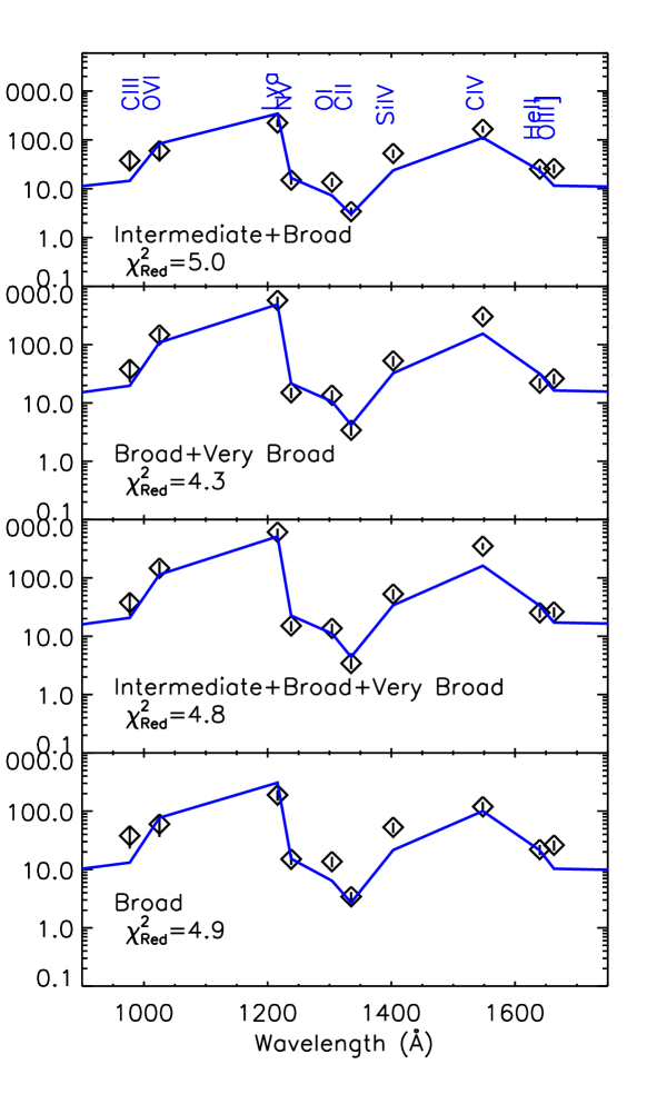
Figure 1: The LOC fitting considering the sum of the broad and very-broad line-components provides consistently a better description of the data for any other choice of parameters. From top to bottom: combination of intermediate+broad, broad+very-broad, intermediate+broad lines+very-broad and broad lines alone. In this example, we only show the fit to the UV data.

3.2 The LOC fitting

The best-fit distribution of the gas in the black hole system is dependent on many parameters using the LOC model. The radial distribution and the covering factor of the gas, which are the free parameters in the fit, in turn depend on pre-determined parameters, namely the SED, the metallicity (that we assume to be solar for the moment, see Sect. 4.1), and the inner and outer radii of the gas. Moreover, broad lines measured in an energy range covering more than three decades in energy, are likely to arise from gas distributed over a large region with inhomogeneous characteristics.

In fitting our model, we considered four different UV line-widths combinations, namely intermediate+broad, broad+very broad, intermediate+broad+very broad as well as broad lines alone (Table 1). We also selected six bands over which to perform the $\chi^{2}$ test on the line flux modeling i.e. optical, X-rays, UV, optical+UV, X-rays+UV and X-rays+UV+optical. The individual bands are defined by the instruments used (Table 1). We used an array of six possible inner radii, ranging from log $r$=14.75 to 17.7 cm (the actual outer radius being log $r$=18.5 cm) to construct the model. Considering all combinations of parameters, we obtain 144 different fitting runs. Whenever a limited number of lines (e.g. the UV band lines alone) are fitted, the model is extrapolated to the adjacent bands to inspect the contribution of the best-fit model to the other lines. Not all the runs are of course sensitive to all the parameters. For instance a run which fits the X-ray band only will be insensitive to any UV line widths. Free parameters of the fit are the covering factor $C_{V}$ of the gas and the slope $\gamma$ of the radial distribution. The covering factor ($\Omega/4\pi$, where $\Omega$ is the opening angle) measured by the LOC is the fraction of the gas as seen by the source. The value of $C_{V}$ is constrained to lie in the range 0.05–0.6, based on the range of past estimates for the BLR obtained with different techniques (see Sect. 4.3). In the following we describe the dependence of the fit on the different parameters, based on the goodness of fit.

In Fig. 1 we show the comparison among best-fits with different line widths for the UV lines. Considering the same band (the UV only here), the inclusion of the intermediate component (Sect. 2.2) systematically slightly worsen the fit. For simplicity, in the following we describe the sum of the broad and very broad components only, as they provide a slightly better fit, although the other combinations were also always checked in parallel.

We show the fits in the different wavelength bands in Fig. 2. In Table 2 the best fit parameters are shown for each combination of bands, using the full range of radii. We note that the UV data certainly dominate the fit, by virtue of the larger number of data points with a relatively smaller error bar. The global fit however does not completely explain the high- and low-energy ends of the data. A fit based on the X-ray data under-predicts the UV and optical data, maybe suggesting the presence of an additional component. On the other hand, the fit based on the optical band, well describes both the optical and the C iv UV line, albeit with a large overestimate of the rest of the UV and X-ray lines.

The LOC fitting depends also on the inner radius over which the radial gas distribution is calculated. We fitted the data for a choice of six inner radii, roughly separated by half a decade. In Fig. 3 a fit considering all the data is plotted for a selection of inner radii. We see that while the UV band is only marginally affected by the inner radius choice, this parameter can make a difference for the optical and X-ray bands.

The application of a a single component of the LOC model with some tunable parameters, does not totally explain the data. In the following we explore other effects that may play a role in the line emission.

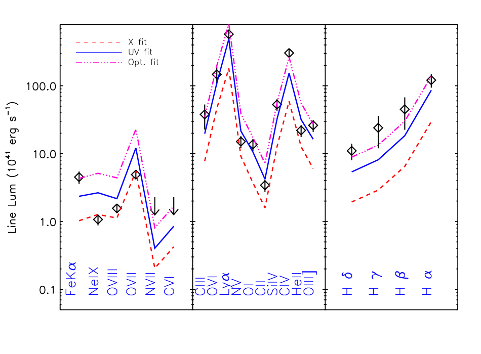
Figure 2: LOC fits over individual bands: X-rays (dashed line), UV (solid line) and optical band (dash-dotted line).

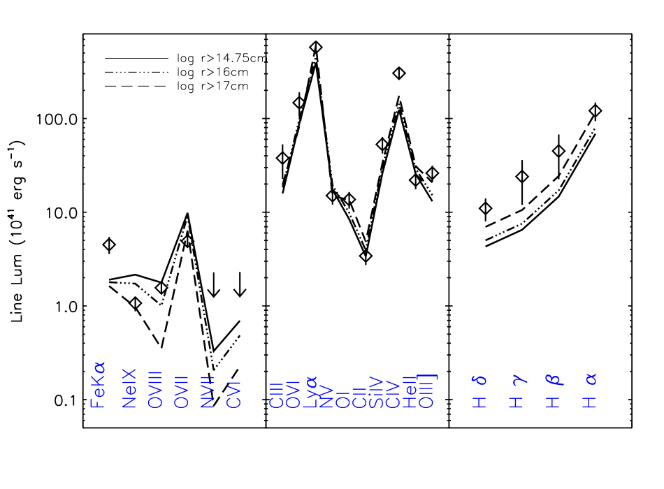
Figure 3: LOC fits over the whole spectral band (X-UV-optical) with three representative inner radii. The X-ray band is best fitted for smaller inner radii, while the Optical band may be better described if larger radii are used.

Table 2: Results the LOC fitting considering different spectral bands.

	$\gamma$	$C_{V}$	$\chi^{2}_{\rm Red}$ (dof)
O	$1.10\pm 0.5$	$>0.6$	0.9 (2)
UV	$1.05\pm 0.08$	$<0.05$	4.3 (8)
X	$1.13\pm 0.23$	$>0.6$	1.5 (4)
UV+X	$1.05\pm 0.05$	$<0.05$	4.9 (14)
UV+O	$1.0\pm 0.1$	$<0.05$	3.4 (12)
UV+O+X	$1.05\pm 0.06$	$<0.05$	4.4 (18)

Notes: $\gamma$ is the slope of the radial distribution of the line luminosities. $C_{V}$ is the covering factor of the BLR gas. $\chi^{2}_{\rm Red}$ is the reduced $\chi^{2}$ and $dof$ are the degrees of freedom.

3.3 Extinction in the BLR

As seen above, the application of the LOC model to Mrk 509 points out that the optical lines are systematically underestimated. A possible solution is to include extinction in the BLR itself. The UV/optical continuum Mrk 509 is not significantly reddened (Osterbrock, 1977). However, the dust may be associated only to the line emission region, in a way that the continuum that we measure would be unaffected (Osterbrock & Ferland, 2006). In principle, the He ii(1640Å)/He ii(4686Å) ratio would be an indicator of reddening intrinsic to the BLR (e.g. Osterbrock & Ferland, 2006). In practice, both lines are severely blended with neighboring lines and with the wing of higher flux lines, namely C iv for He ii(1640Å) and H$\beta$ for He ii(4686Å) (Bottorff et al., 2002). In our case, the observed line ratio is very low ($\sim 1.7$) when compared to the theoretical value derived from the LOC model (6–8; Bottorff et al., 2002). This line ratio would imply an extinction E(B-V)=0.18 (eq. 4 of Annibali et al., 2010), when a Small Magellanic Cloud (SMC) extinction curve, possibly more appropriate for AGN, is used (Hopkins et al., 2004; Willott, 2005). Knowing the uncertainties (i.e. line blending) associated to our He ii measurements, we took this value as the upper limit of a series of E(B-V) values to be applied to our lines. Namely, we tested E(B-V)=(0.18, 0.15, 0.10, 0.075, 0.05, 0.025). We then corrected accordingly the observed optical and UV fluxes (Annibali et al., 2010). For the lines observed by FUSE (Table 1), we extrapolated the known SMC extinction curve with a $\lambda^{4}$ function to reach those wavelengths. The extinction in the X-rays has been simply estimated using the E(B-V)-$N_{\rm H}$ relation provided in Predehl & Schmitt (1995), considering a SMC-like selective to total extinction ratio $R_{V}$ of 2.93 (Pei, 1992).
When only the UV lines are modeled, the $\chi^{2}$ method chooses lower values of the BLR extinction, with a final $\chi^{2}_{\rm red}$ of 6.1 (dof=8) for E(B-V)=0.025. The effect of the BLR extinction is relatively modest in the X-ray band and mainly affecting the O vii lines. However, any value of the BLR extinction largely overcorrects the Balmer series lines. Therefore when also the optical lines are included in the model, the resulting fit becomes even worse ($\chi^{2}_{red}=16-20$, for 18 dof).

3.4 A two-component LOC model

A single LOC-component does not provide a fully satisfactory fit. This is not surprising, given the large range of ionization potentials of the lines. Therefore we attempt here to test a two-component model. As before, for each of the two components we fit all the combinations of line widths (as in Fig. 1). We first considered the whole range of radii (Model 1 of Table 3). Then we made the inner radius (as defined in Sect. 3.2) of both components vary (Model 2 in Table 3). Finally, we took into account the different emissivity depending on the size of the region, by varying also the outer radius. To do this, we divided the radial range into four regions (starting at log$r=14.75,15.53,16.56,17.47$), in order to have roughly an order of magnitude difference between two adjacent radii. We then considered for each component all combination of adjacent regions (or single regions). Therefore we have a total of 10 options for the size of each component of the gas (Model 3 in Table 3). Note that for each run the inner and outer radii were fixed parameters. We fitted the whole band (X-ray, UV, optical: XUVO) for the two LOC components. The fit is driven by the UV band, where the uncertainties on the data are the smallest. We note that the slope of the powerlaw is dependent on the covering factor, as flatter slopes ($\gamma<1.1$) systematically correspond to very small covering factors ($C_{V}<0.05$). Conversely, the upper limit we set for the covering factor ($C_{V}$=0.6) corresponds to steeper radial slopes (see also Korista & Goad, 2000). The covering factor has the effect of regulating the predicted line luminosities. A steeper radial distribution would enhance the lines at smaller radii, where the gas illumination is stronger. Therefore a larger $C_{V}$ would be required to tune down the line luminosities. On the contrary, a flatter slope, would lower the contribution of the strong-illuminated region, while the outer radii are enhanced. However, the radiation field lowers with the distance, therefore a smaller $C_{V}$ is necessary to adapt the predicted fluxes to the real data. In the last line of Table 3 we report the reduced $\chi^{2}$. The reduced $\chi^{2}$ never falls below $\sim$2, even for the better-fitting models. This is especially due to the outlying data points, namely Si iv, C iv, and He ii. The exclusion of the Fe K$\alpha$ was not resolutive, as this line has a larger uncertainty with respect to the UV lines. Fig. 4 refers to Model 3. As expected, the more sensitive lines were the optical and the X-rays, respectively. A highly ionized component, extending down to log$r<$14.7 cm is necessary in order to reproduce the O viii and Ne ix lines in the X-rays. All the optical lines and part of the C iv line are best fitted by adding a component with a larger inner radius.

Table 3: Best fit parameters for a two-component model and different emitting regions.

	Model 1	Model 2	Model 3
Comp 1
$r_{in}$	14.75	17.0	17.47
$r_{out}$	18.5	18.5	18.5
$\gamma$	$1.59\pm 0.03$	$1.04\pm 0.02$	$1.10\pm 0.02$
$C_{V}$	$<0.05$	$<0.05$	$>0.6$
Comp 2
$r_{in}$	14.75	14.75	14.75
$r_{out}$	18.5	18.5	17.47
$\gamma$	$1.06\pm 0.02$	$1.17\pm 0.02$	$1.15\pm 0.02$
$C_{V}$	$<0.05$	$>0.6$	$>0.6$
$\chi^{2}_{red}$ (dof)	5.2(15)	2.5(15)	2.3(15)

Notes:
The parameters are: $r_{in}$, the inner radius; $r_{out}$ the outer radius; $\gamma$, the slope of the radial distribution and $C_{V}$, the covering factor. Note that the Fe K$\alpha$ line is excluded from this fit. model 1: the emissivity occurs over all radii for both components.
model 2: the two components have different inner radii.
model 3: both the inner and outer radii of the emissivity is variable for both components.

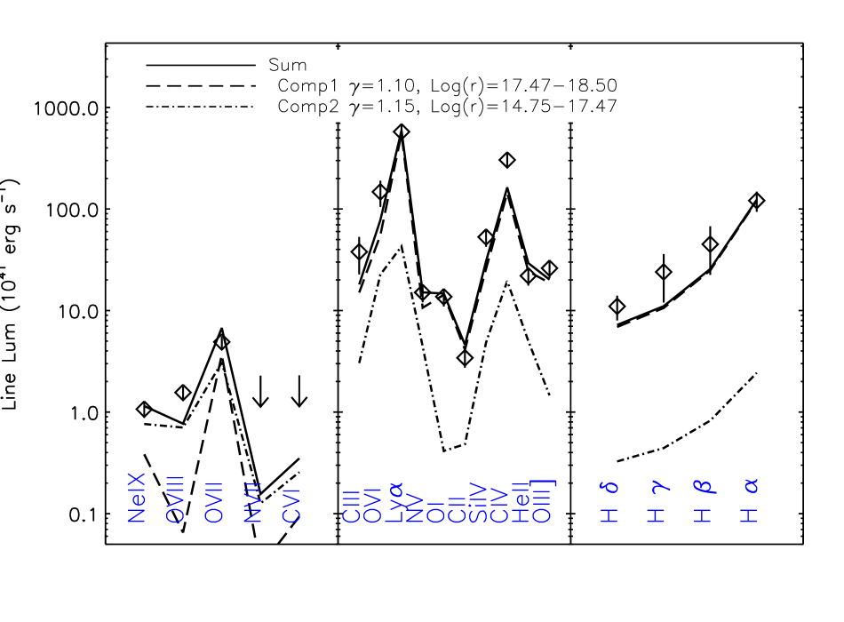
Figure 4: Upper panel: LOC fit with two components, acting in different regions near the AGN (Model 3 in Table 3). X-ray data are best fitted by a component near the black hole, while the optical data are better fitted by a further-away component. Lower panel: residuals to the fit.

4 Discussion

4.1 Abundances and the influence of the SED

Abundances in the BLR should be either solar or super-solar. The metal enrichment should come from episodic starburst activity (Romano et al., 2002). The N v line is often taken as an abundance indicator in AGN since it is a product of the CNO cycle in massive stars. Using the broad component ratios in our data for N v/C iv and N v/He ii, the diagnostic plots of Hamann et al. (2002) suggest abundances in Mrk 509 of $1<Z<3$ (see Steenbrugge et al., 2011, for the limitations in determining abundances in the BLR). In this analysis we considered a SED with solar abundances, as defined in Cloudy. We therefore also tested the fits presented above using a metallicity 3 times solar. The fits obtained are systematically worse ($\Delta\chi^{2}=2-7$ for the same number of degrees of freedom). This suggests that the abundances are close to solar.

The present HST-COS data were taken 20 days after the last XMM-Newton pointing (Kaastra et al., 2011), as the closing measurements of the campaign, which lasted in total about 100 days. Spectral coverage simultaneous to HST-COS was provided instead by both Chandra-LETGS (Ebrero et al., 2011) and Swift-XRT (Mehdipour et al., 2011). We used the average SED recorded, 20–60 days before the HST-COS observation, by the XMM-Newton instruments. The choice of SED is very important in the BLR modeling, as different lines respond on different time scales to the continuum variations (Korista & Goad, 2000; Peterson et al., 2004). Reverberation mapping studies of Mrk 509 report that the delay of the H$\beta$ with respect to the continuum is very long (about 80 days for H$\beta$, Carone et al., 1996; Peterson et al., 2004). However, higher ionization lines respond faster to the continuum variations. Taking as a reference the average H$\beta$/C iv delay ratio for NGC 5548 (Peterson et al., 2004), for which, contrary to Mrk 509, a large set of line measurements is available, we obtain that the C iv line in Mrk 509 should roughly respond in 40 days. A similar (but shorter) time delay should apply to the Ly$\alpha$ line (Korista & Goad, 2000). This delay falls in the time interval covered by the XMM-Newton data. Therefore our choice of SED should be appropriate for the modeling of at least the main UV lines. Variability of the X-ray broad lines has been reported on years-long time scales (Costantini et al., 2010), however no short-term studies are available. We expect that the X-ray broad lines should respond promptly to the continuum variations, as they may be located up to three times closer to the black hole with respect to the UV lines (C07). During the XMM-Newton campaign the flux changed at most 30%, with a minimal change in spectral shape (Sect. 3.1). The used SED should therefore represent what the BLR gas see for the X-ray band. However, for the optical lines the used SED might be too luminous as the we observed an increase in luminosity by about 30% during the XMM-Newton campaign, and as seen above, the time-delay of the optical lines may be large.

4.2 The UV-optical emitting region

The LOC model has been extensively used to model the UV and optical lines of AGN (e.g. Korista et al., 1997a). In this study we find that a single radial distribution of the gas over the whole range of radii, applied to the UV band, would have a slope $\gamma\sim 1$, as prescribed by the standard LOC model (Table 2). The covering factor is unconstrained as it hits the lower limit that we imposed on this parameter. As in the case of Mrk 279 (C07), the C iv line is a systematic outlier. This line may obey to mechanisms other than pure gravitation (e.g. inflows/outflows) or may arise in a geometrically different region than e.g. the optical lines (e.g. Goad et al., 2012, and references therein). Finally, Ly$\alpha$ and C vi are found in some sources to respond on a slightly different time scale to the continuum variation. In the case of NGC 5548 this difference in response is of the order of 20 days (Korista & Goad, 2000, Sect. 4.1). This may account for some of the mismatch between the two lines in our fit. As tested above (Sect. 3.3), extinction in the BLR of Mrk 509 must be negligible, therefore the discrepancy with the model cannot be ascribed to dust in the emitting region. The ionization of the BLR follows the rules of photoionization. In particular for a given UV-emitting ion (e.g. C iv, Ly$\alpha$, O vi, as detailed in Korista et al., 1997a), the ionization parameter remains constant throughout the region (dashed lines in Fig. 5). Note that for lower ionization lines (namely, the Balmer lines, Fig. 5, right panel), density effects come into play besides pure recombination (Kwan & Krolik, 1979; Osterbrock & Ferland, 2006) and the ionization parameter does not follow the emission contour (Korista et al., 1997a). This model does not require a universal ionization parameter, because of the assumption of the stratified nature of the gas. A pressure confined gas model, which may also allow for a range of ionization parameters in a stratified medium, would also predict, given a bolometric luminosity, a gas hydrogen density as a function of radius (eq 21 in Baskin et al., 2014). This prediction is drawn in Fig. 5 (magenta solid line), using $L_{bol}\sim 3L_{1350\,\AA}$ (Kaspi et al., 2005), where $L_{1350\,\AA}$ has been extrapolated from the average SED of Mrk 509 (Kaastra et al., 2011). This density prediction is not too far off, however it overestimates the optimal emitting region density of the higher ionization ions (an example is given in the left panel of Fig. 5), while it would match the Balmer lines emitting region (right panel).

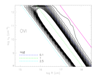
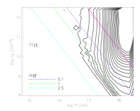
Figure 5: contour profiles of O vi and H$\alpha$ as a function of density and distance, here using a radial slope $\gamma$ of 0.10. The dashed lines indicates constant ionization parameters, as detailed in the legend. The solid magenta line follows the density prediction of the pressure confined emission model of Baskin et al. (2014).

4.3 The size and gas distribution of the BLR

Several arguments point to a natural outer boundary for the BLR which should be intuitively given by the dust sublimation radius (Suganuma et al., 2006; Landt et al., 2014). For Mrk 509, this radius corresponds to $3.6\times 10^{18}$ cm (Mor & Netzer, 2012).

The maximum radius of our LOC model is $3\times 10^{18}$ cm. An expansion of the BLR outer radius to $7.6\times 10^{18}$ cm does not improve the fit. This is a natural consequence of the LOC model construction. For radial distributions with slopes $\gamma\raisebox{-2.15277pt}{$\;\stackrel{{\scriptstyle>}}{{\sim}}\;$}1$ the line emissivity of some major lines (O vi, C iv) already drops at $10^{18}$ cm (C07, Baskin et al., 2014). Therefore our fit is consistent with a confined BLR region, possibly within the sublimation radius.

The radius of the BLR has been found to scale with the UV luminosity. If we take the C iv line as a reference, $R_{\rm BLR}=2\times 10^{16}h_{0}L_{42}^{0.5}$(C iv), where $h_{0}$ is the Hubble constant in units of 100 km s^-1 and $L_{42}$ is the C iv luminosity in units of $10^{42}$ erg s^-1 (Peterson, 1997). For Mrk 509, the radius of the BLR based on this equation is $\sim 2.6\times 10^{17}$ cm. Using instead the known relation between the size of the H$\beta$ emitting region and the luminosity at 5100Å, we obtain, for Mrk 509, $R_{{\rm H}\beta}\sim 1.2\times 10^{17}$ cm (Bentz et al., 2013).
In our fit the location of the UV emitting lines is consistent with these estimates, as, although UV lines are efficiently emitted in a large range of radii (Fig. 3 and C07), a large fraction of the UV line luminosity could come from radii $\geq 10^{17}$ cm (Model 2,3 in Table 3, Fig. 4). Assuming Keplerian motion, the FWHM of our lines imply that the very-broad lines (FWHM$\sim$9000-10,000 km s^-1) are located at approximatively $2.5-5\times 10^{16}$ cm, depending on the mass of the black hole: $1.43\times 10^{8}$ M_⊙ (Peterson et al., 2004) or $3\times 10^{8}$ M_⊙ (Mehdipour et al., 2011). For the broad lines (FWHM$\sim$4000-5000 km s^-1) the distance would then be $1.3-2.5\times 10^{17}$ cm, consistent with our results for the UV-optical component. Finally for the intermediate lines (FWHM$\sim$1000-3000 km s^-1) the calculated distance is $2-4\times 10^{18}$ cm. The location of the line emitting gas is stratified, therefore these single-radius estimates are only taken as a reference. The very-broad and the broad lines are well within the estimated radius for the BLR. The so-called intermediate line region could possibly bridge the BLR and the NLR (Baldwin, 1997).

In interpreting the BLR emission, we tested a two-component model, characterized not only by different radial distributions and covering factors, but also by different physical sizes and inner/outer radii of the emitting plasmas.

Our fits are not completely satisfying as important outliers, like C iv, are present. However, the best fit points to the interesting possibility that the optical and part of the UV region originates at larger radii (starting at $3\times 10^{17}$ cm), while the X-ray- and some fraction of the UV-emission regions would have an inner radius smaller than $6\times 10^{14}$ cm (as also found in C07) and a larger extension up to about the beginning of the optical BLR (Sect. 3.4). This would point to a scenario in which the optical lines, including the H$\beta$, would come from the outer region of the BLR. Such a span in distance between the optical and the X-ray lines, would also imply for the latter a faster response-time to any continuum variation. Such an effect has not been systematically studied, although strong flux variation of the O vii broad line has been observed before (Costantini et al., 2010). The inability to find a good fit with the present model, which assumes a simple plane parallel geometry, could suggest a more complex geometry. Recently for instance an inflated geometry (”bowl geometry”, Goad et al., 2012) for the outer region, possibly confined by a dusty torus has been suggested using different approaches (Goad et al., 2012; Pancoast et al., 2012; Gaskell & Goosmann, 2013).

The covering factor was set in our fits to be in the range 0.05–0.6. The lower limit has been chosen following early studies on the relation between the equivalent width of the Ly$\alpha$ and the covering factor (0.05–0.1, e.g. Carswell & Ferland, 1988). However subsequent studies, using among others also the LOC model technique, have pointed out that the covering factor can be larger: from 0.30 (e.g. Maiolino et al., 2001, and references therein) up to 0.5–0.6 (Korista & Goad, 2000). The covering factor here is the fraction of the gas as seen by the source. This is equal to the observer’s line of sight covering factor only if a spherical distribution of the gas is assumed. A more flattened geometry would then reconcile a large covering factor with the fact that absorption lines from the broad line region are in general not observed in the optical-UV band. In our fits the covering factor is unconstrained. However large covering factors have been preferentially found when a two-component model was applied, especially when the inner and outer radius were allowed to vary for both components. The measured high covering fraction, necessary to explain the line luminosities of the two components, would then point to a gas with non-spherical geometry. As these two components are along our line of sight, they may be one below the other, therefore the sum of the two $C_{V}$ can well be above one, as long as the individual covering factors do not cover entirely the source (i.e. $C_{V}<1$).

Despite the extensive exploration of the impact of different parameters to the modeling, our analysis also underlines that a simple parameterization may be inadequate to explain the complexity of the BLR. Reasons for not reaching a better fit include minor effects like possible different responses of Ly$\alpha$ and C iv to continuum variations, non-simultaneity of the FUSE data, and inhomogeneous information on the broad-band line profiles. The $C_{V}$ may not be a simple step function, but the clouds/gas-layers may experience a differential covering factor for instance as a function of the distance or line ionization. A major effect would be the complex dynamics and geometry of the BLR, which needs more sophisticated models to be explained.

4.4 The iron line at 6.4 keV

In this paper we include the 6.4 keV Fe K$\alpha$ line, observed simultaneously with the other soft X-ray, UV and optical lines. The narrow and non-variable component, probably produced in distant regions, was not considered in the fit. We find that the derived emission of the BLR contribution to the broad Fe K$\alpha$ line component is around 30%, if we used a two-component model. The emission would happen at a range of distances from the source, although at small radii (log$r\raisebox{-2.15277pt}{$\;\stackrel{{\scriptstyle>}}{{\sim}}\;$}$14.75 cm) the emission is enhanced (Fig. 3). Note that fortuitously, a single component fit, based on the optical lines, would provide a perfect fit to the Fe K$\alpha$ line (Fig. 2). However, such a gas would produce both UV and soft-X-ray line fluxes at least a factor of 6 larger than observed. A modest contribution ($\sim 17\%$) of the BLR to the iron line has been also reported in Mrk 279, using non simultaneous UV and X-ray data (Costantini et al., 2010).

5 Conclusions

In this paper we attempted to find a global explanation of the structure of the gas emitting broad lines in Mrk 509, from the he optical to the X-ray band using a simple parametrization of the BLR. This study is possible thanks to the simultaneous and long observations of XMM-Newton and HST-COS.

We find that lines broader than FWHM$>$4000 km s^-1 contribute to the bulk of the BLR emission. A two-component LOC model provides a statistically better, but not conclusive, description of the data. The two components are characterized by similar radial emissivity distribution ($\gamma\sim 1.10-1.15$), but different size and distance from the central source. The X-rays and part of the UV radiation come from an inner and extended region ($r\sim 5\times 10^{14}-3\times 10^{17}$ cm), while the optical and part of the UV gas would be located at the outskirts of the BLR ($r\sim 3\times 10^{17}-3\times 10^{18}$ cm). This picture appears to be in agreement with recent results on the geometry of the BLR, locating the H$\beta$ line away from the ionizing source. However, more sophisticated parameterizations are needed to have a definitive answer.

The Fe K$\alpha$ broader line cannot completely be accounted for by emission from the BLR gas. The contribution of the BLR is around 30% for this line.