Domain formation in membranes near the onset of instability

Abstract

The formation of microdomains, also called rafts, in biomembranes can be attributed to the surface tension of the membrane. In order to model this phenomenon, a model involving a coupling between the local composition and the local curvature was proposed by Seul and Andelman in 1995. In addition to the familiar Cahn-Hilliard/Modica-Mortola energy, there are additional ‘forces’ that prevent large domains of homogeneous concentration. This is taken into account by the bending energy of the membrane, which is coupled to the value of the order parameter, and reflects the notion that surface tension associated with a slightly curved membrane influences the localization of phases as the geometry of the lipids has an effect on the preferred placement on the membrane.

The main result of the paper is the study of the $\Gamma$-convergence of this family of energy functionals, involving nonlocal as well as negative terms. Since the minimizers of the limiting energy have minimal interfaces, the physical interpretation is that, within a sufficiently strong interspecies surface tension and a large enough sample size, raft microdomains are not formed.

Keywords: $\Gamma$-convergence, nonlocal energies, interpolation.

AMS Mathematics Subject Classification: 49J45, 74K15.

1 Introduction

The continuum theory of membranes has been an active area of research in material and biological sciences since the pioneering works of Canham and Helfrich, [6, 17]. Biological cell membranes or biomembranes are complex structures commonly made up of lipids, proteins, and cholesterol. Of recent very widespread interest is the phase separation and domain formation of these compounds forming the cell membrane. The resulting nanoscale microdomains, referred to as ‘lipid rafts’, are believed to be responsible for membrane trafficking, intracellular signaling, and assembly of specialized structures, [33]. Many important biological processes, such as virus budding, endocytosis, and immune responses, are believed to be linked to membrane rafts, [29]. Ever since the first experimental evidence of raft formation in late 1980’s, there has been a growing body of literature on both theoretical and experimental aspects of this phenomenon, [11]. However, due to very small scales associated with raft domains (they are too small to be optically resolved) [29, 5, 25], there are different viewpoints on the precise structure and stability of lipid rafts, [24]. As a result, understanding the conditions for the formation, as well as mechanisms driving stability (and instability), of these microdomains is of great importance.

It has been proposed in [22] that raft formation can be attributed to the surface tension of the membrane. The experimental basis for the theory comes from the work of Rozovsky et al in [31], in which domain formation in a ternary mixture of sphingomyelin, DOPC, and cholesterol is observed for a vesicle adhered to a substrate structure. To study the relation between an increase in surface tension and the morphological transitions on the membrane plane, a coupling between the local composition and the local curvature was proposed in [22]. The authors consider a free energy framework and use an energy functional first introduced in [32] to model phase separation of a di-block copolymer in a membrane allowing out of plane (bending) distortions (see also [20, 34, 23]).

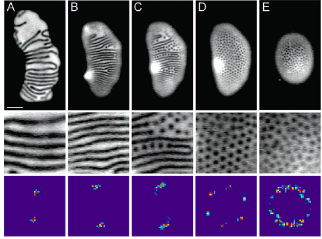
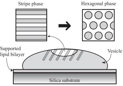
Figure 1: Experimental and schematic representation of rafts. The first picture is reprinted with permission from S. Rozovsky, Y. Kaizuka, and J. T. Groves. Formation and spatio-temporal evolution of periodic structures in lipid bilayers. J. Am. Chem. Soc., 127(1):36–37, 1 2005. Copyright 2005 American Chemical Society. It depicts epifluorescence microscopy images of phase separation in a vesicle composed of a mixture of sphingomyelin, DOPC, and cholesterol adhering to a supported lipid bilayer. Rafts, initially forming a stripe pattern evolve into a hexagonal array of circular domains as the vesicle changes shape. The last row depicts Fourier spectra for the ordered regions depicted in the middle row. The second picture, showing a schematic representation of the same process, is reprinted with permission from S. Komura, N. Shimokawa, and D. Andelman. Tension-induced morphological transition in mixed lipid bilayers. Langmuir, 22:6771–6774, 2006. Copyright 2006 American Chemical Society.

Similar to the classic Ginzburg-Landau models, the system is described in terms of an order parameter $u$ that may, for instance, model the relative composition of the lipids and cholesterol on the membrane plane. However, in addition to the familiar Cahn-Hilliard/Modica-Mortola energy (see [27]),

$$\mathcal{A}_{\varepsilon}[u]:=\int_{\Omega}\left(\frac{1}{\varepsilon}W(u)+\varepsilon|\nabla u|^{2}\right)dx,$$ (1.1)

that models line tension between domains and represents ‘short-range’ interactions and whose minimization drives the system to evolve into $A$ rich and $B$ rich phases (corresponding to $u=\alpha$ or $u=\beta$, minima of a double-well potential $W$), there are additional ‘forces’ that prevent large domains of homogeneous concentration. In [32] Seul and Andelman proposed a nonlocal contribution to the energy by considering an energy functional that takes into account the bending energy of the membrane, and couples it to the value of the order parameter. The idea is that surface tension associated with a slightly curved membrane influences the localization of phases as the geometry of the lipids has an effect on the preferred placement on the membrane. Similarly, the geometry of the membrane may adapt to that of the molecules. The resulting energy has the form

$$\mathcal{E}[\phi,h]=\int_{D}\left(f(\phi)+\frac{1}{2}b|\nabla\phi|^{2}+\frac{1}{2}\sigma|\nabla h|^{2}+\frac{1}{2}\kappa(\Delta h)^{2}+\Lambda\phi\Delta h\right)d\bar{x}.$$ (1.2)

Here $D:=\{Lx:x\in\Omega\}$ is the domain with the characteristic size $L$, $\phi$ is the order parameter, $h$ represents the height profile of the membrane, $f(\phi):=\frac{a_{2}}{2}\phi^{2}+\frac{a_{4}}{4}\phi^{4}$, where $a_{2},a_{4}$ are constants, $b>0$ is related to the line tension between different domains, $\sigma>0$ and $\kappa>0$ are the surface tension and bending rigidity of the membrane, respectively, and $\Lambda$ is the composition-curvature coupling constant.

Symbol	Description	Value
$a_{4}$		$10^{-5}J/m^{2}$
$b$	line tension	$5\times 10^{-19}J$
$\sigma$	surface tension	$5\times 10^{-6}$ to $10^{-4}J/m^{2}$
$\kappa$	bending rigidity of the membrane	$10^{-19}J$
$\Lambda$	composition-curvature coupling constant	$4.9\times 10^{-12}J/m$

Table 1: Parameter descriptions and characteristic values, [22].

We note that several simplifying assumptions have been made in relation to the classical membrane energies (e.g. [6, 17]) or more recent multi-component biological membrane energies (e.g. [15]). Rather than considering a closed hypersurface to represent the vesicle. We assume that the vesicle is almost flat and that its shape is described in terms of the distance, $h$, to the reference plane, $D\subset\mathbb{R}^{2}$. In addition, for simplicity, higher-order coupling terms between the composition and the curvature of the membrane are omitted. There is no direct measure of the resulting single coupling parameter, $\Lambda$, but it can be fitted based on experimental data (see [22] for details).

Since minimizers of $\mathcal{E}$ satisfy the Euler-Lagrange equations, we may consider the minimization problem for $\mathcal{E}[\phi,h]$ under the constraint, $\frac{\delta\mathcal{E}}{\delta h}=0$. Using the last equation to eliminate $h$ (see the Appendix) and rescaling

$$u(x)=\phi(Lx),\quad\varepsilon:=\sqrt{\frac{\kappa}{L^{2}\sigma}},\quad q:=1-\frac{b\sigma}{\Lambda^{2}},\quad W(u):=\frac{2\kappa}{\Lambda^{2}}f(u),\mbox{\quad and\ }{\mathcal{F}}^{\ast}_{\varepsilon}:=\frac{1}{\varepsilon}\frac{2\kappa}{\Lambda^{2}L^{d}}\mathcal{E},$$

one can reduce (1.2) to

$${\mathcal{F}}^{\ast}_{\varepsilon}[u]:=\frac{1}{\varepsilon}\int_{\Omega}\left(W(u)-u^{2}+(1-q)\varepsilon^{2}|\nabla u|^{2}+u\left({\bf 1}-\varepsilon^{2}\Delta\right)^{-1}u\right)\,dx.$$ (1.3)

Here $q$ is a constant parameter and the second order differential operator ${\bf 1}-\varepsilon^{2}\Delta:H^{2}(\Omega)\rightarrow L^{2}(\Omega)$ is subject to Neumann boundary conditions. A detailed derivation is given in the Appendix. In addition, Table 1 lists typical values for the parameters. Note that $\sqrt{\frac{\kappa}{\sigma}}\sim 10^{-7}m$, so the domain size of $10$ microns corresponds to $\varepsilon\sim 10^{-2}$. One may also easily check from the table that the relevant values of the parameter $q$ fall in the interval $(-1.1,1)$, and for fixed $b$ and $\Lambda$ correspond to varying the surface tension.

Moreover, the line tension, surface tension, and the composition-curvature coupling constant are embedded in the effective parameter $q$. To develop some intuition about the effect of varying $q$ we momentarily assume dependence only on a single direction and consider the energy of a single term in the Fourier series expansion of $u$ (see the Appendix),

$$u(x)=\psi_{n}(x),\qquad x\in\Omega=(-1,1),$$

where

$$\psi_{n}(x):=\cos(\lambda_{n}x)\quad\text{and}\quad\lambda_{n}=2\pi n.$$

Then,

$$({\bf 1}-\varepsilon^{2}\Delta)^{-1}\psi_{n}=\frac{1}{1+\varepsilon^{2}\lambda_{n}^{2}}\psi_{n},$$

and separating the potential term in the energy we have,

$${\mathcal{F}}_{\varepsilon}^{*}[\psi_{n}] =\frac{1}{\varepsilon}\int_{-1}^{1}W(\psi_{n})dx+\frac{1}{\varepsilon}\int_{-1}^{1}\left(-1+(1-q)\varepsilon^{2}\lambda_{n}^{2}+\frac{1}{1+\varepsilon^{2}\lambda_{n}^{2}}\right)\cos^{2}(\lambda_{n}x)dx$$

$$=\frac{1}{\varepsilon}\int_{-1}^{1}W(\psi_{n})dx+\frac{1}{\varepsilon}{\mathcal{F}}_{q,n},$$ (1.4)

where

$${\mathcal{F}}_{q,n}:=-1+(1-q)\varepsilon^{2}\lambda_{n}^{2}+\frac{1}{1+\varepsilon^{2}\lambda_{n}^{2}}.$$ (1.5)

For fixed $q>0$, the minimum of ${\mathcal{F}}_{q,n}$ is achieved by

$$\varepsilon^{2}\lambda_{n_{*}}^{2}=\frac{1}{\sqrt{1-q}}-1,$$

with the corresponding energy

$${\mathcal{F}}_{q,n_{*}}=-2+2\sqrt{1-q}+q<0.$$ (1.6)

As evident from the calculations above, the contribution to the full energy from ${\mathcal{F}}_{q,n_{*}}$ becomes negative as $q$ increases from $0$ (corresponding to the weakening tension). Hence, depending on the properties of the potential $W$ the functional may be unbounded from below. A natural question is to understand this bifurcation as $q$ increases. This paper represents a step towards that goal. In particular, we show that for a standard family of double-well potentials (see Hypotheses 2.2), even if $q$ is positive, the energy is bounded from below and $\Gamma$-converges to the perimeter functional for $q$ sufficiently small. Since the minimizers of the limiting energy have minimal interfaces, the physical interpretation is that for $L^{2}\gg\kappa/\sigma$, $(\varepsilon\ll 1)$ raft microdomains are not formed in this regime. If the surface tension is too small and the functional is unbounded from below as $\varepsilon\rightarrow 0$, different mathematical methods will have to be used to study the formation of raft-like microdomains (e.g. [26, 28]).

We remark that when $q\leq 0$ the $\Gamma$-convergence to the perimeter functional can be proved under weaker conditions on the potential. In that case the functional is nonnegative (this can be seen from the reformulation of the problem presented in (2.1)). The $\Gamma$-convergence of similar energies has been considered before (e.g. [18, 2]), however there are some differences with the functional (2.1) (for example when $q=0$) and will be addressed in a separate paper.

Finally, we observe that in our context the relevant physical dimension is $d=2$, although the analysis presented here is carried out in arbitrary dimension $d\geq 2$.

2 Preliminaries, Notation, and Statement of Results

A natural mathematical framework for studying the asymptotic behavior of the family of functionals (1.3) is the notion of $\Gamma$-convergence introduced by De Giorgi in [14] (see also [4, 10]). In a general metric space setting the definition is given below.

Definition 2.1.

Let $(Y,d)$ be a metric space and consider a sequence $\{{\mathcal{F}}_{n}\}$ of functionals ${\mathcal{F}}_{n}$: $Y\rightarrow[-\infty,\infty]$. We say that $\{{\mathcal{F}}_{n}\}$ $\Gamma$-converges to a functional ${\mathcal{F}}:Y\rightarrow[-\infty,\infty]$ if the following properties hold:

1. (Liminf Inequality) For every $y\in Y$ and every sequence $\{y_{n}\}\subset Y$ such that $y_{n}\rightarrow y$,

   $${\mathcal{F}}[y]\leq\liminf_{n\rightarrow\infty}{\mathcal{F}}_{n}[y_{n}].$$

2. (Limsup Inequality) For every $y\in Y$ there exists $\{y_{n}\}\subset Y$ such that $y_{n}\rightarrow y$ and

   $$\limsup_{n\rightarrow\infty}{\mathcal{F}}_{n}[y_{n}]\leq{\mathcal{F}}[y].$$

The functional ${\mathcal{F}}$ is called the $\Gamma$-limit of the sequence $\{{\mathcal{F}}_{n}\}$.

A key property of $\Gamma$-convergence is the fact that, under appropriate compactness conditions, the sequence of minimizers of the functionals ${\mathcal{F}}_{n}$ converge to a minimizer of the limiting functional ${\mathcal{F}}$. Moreover, one can show that the isolated local minima of the $\Gamma$-limit ${\mathcal{F}}$ persist under small perturbations (see [21, 10]).

The problem of finding a characterization of the $\Gamma$-limit of (1.3) has been considered in the one-dimensional setting by Ren and Wei in [30], but in a different parameter regime. Due to the different scaling of the terms, the technique used in that paper is not applicable to our case. Recall that the last term in (1.3) renders the problem nonlocal. A local approximation of (1.3) was studied in [7] and [8]. We refer to the derivation of (6.27) in the Appendix for the precise connection between the models. Qualitative properties of local minimizers of the local approximation model have been studied extensively to explain the formation of periodic layered structures (see [3, 9, 26, 28]).

We now give the precise formulation of our results. Let $\Omega\subset\mathbb{R}^{d}$, $d\geq 2$, be an open, bounded set of class $C^{2}$, and let $W$ be a twice continuously differentiable double-well potential defined on the real line. We make the following hypotheses on $W$.

Hypotheses 2.2.

1. $W(s)>0$ if $s\neq\pm 1$.

2. $W(\pm 1)=0$.

3. There exists $c_{w}>0$ such that $W(s)\geq c_{w}(s\mp 1)^{2}\mbox{ for }\pm s\geq 0.$

4. There exist constants $K_{w}$, $C_{w}>0$ such that $|W^{\prime}(s)|\leq C_{w}\sqrt{W(s)}$ and $|W^{\prime\prime}(s)|\leq K_{w}$ for all $s\in\mathbb{R}$.

Remark 2.3.

Note that conditions 3 and 4 imply that $W$ has quadratic growth at infinity.

For the purposes of our analysis it will be convenient to rewrite the functional ${\mathcal{F}}^{\ast}_{\varepsilon}$ as follows. Given $u\in W^{1,2}(\Omega)$, we define $v\in W^{3,2}(\Omega)$ via

$$-\varepsilon^{2}\Delta v+v=u\text{ in }\Omega\text{ \qquad and\qquad}\frac{\partial v}{\partial n}=0\text{ on }\partial\Omega,$$

where $n$ denotes the outward unit normal to $\partial\Omega$, and use the abbreviatory notation $v:=({\bf 1}-\varepsilon^{2}\Delta)^{-1}u$. Integrating by parts we obtain

$${\mathcal{F}}^{\ast}_{\varepsilon}[u] =\int_{\Omega}\left(\frac{1}{\varepsilon}W(u)-\varepsilon q|\nabla u|^{2}+\varepsilon^{3}(\Delta v)^{2}+\varepsilon^{5}|\nabla\Delta v|^{2}\right)dx$$

$$=\int_{\Omega}\left(\frac{1}{\varepsilon}W(u)-\varepsilon q|\nabla v|^{2}+(1-2q)\varepsilon^{3}(\Delta v)^{2}+(1-q)\varepsilon^{5}|\nabla\Delta v|^{2}\right)dx.$$

Hence, we may also view ${\mathcal{F}}^{\ast}_{\varepsilon}$ as ${\mathcal{F}}_{\varepsilon}[v]$ with ${\mathcal{F}}_{\varepsilon}:L^{2}(\Omega)\rightarrow(-\infty,\infty]$ given by

$${\mathcal{F}}_{\varepsilon}[v]:=\left\{\begin{array}[]{ll}{\mathcal{F}}_{\varepsilon}[v;\Omega]&\mbox{if }v\in W^{3,2}(\Omega),\frac{\partial v}{\partial n}=0\text{\ on\ }\partial\Omega,\\ +\infty&\text{otherwise},\end{array}\right.$$ (2.1)

where

$${\mathcal{F}}_{\varepsilon}[v;A]=\int_{A}\left(\frac{1}{\varepsilon}W(-\varepsilon^{2}\Delta v+v)-\varepsilon q|\nabla v|^{2}+(1-2q)\varepsilon^{3}(\Delta v)^{2}+(1-q)\varepsilon^{5}|\nabla\Delta v|^{2}\right)dx$$

for every open set $A\subset\Omega$.

Remark 2.4.

Observe that if $v\in W^{3,2}(\Omega)$ does not satisfy Neumann boundary conditions on $\partial\Omega$, then ${\mathcal{F}}_{\varepsilon}[v;\Omega]<{\mathcal{F}}_{\varepsilon}[v]=\infty$.

Definition 2.5.

Given a vector $\nu\in\mathbb{S}^{d-1}$ ($d-1$ dimensional unit sphere), let $\{\nu_{1},\cdots,\nu_{d-1},\nu\}$ be an orthonormal basis of $\mathbb{R}^{d}$. We will denote by $Q_{\nu}$ an open unit cube centered at the origin with two of its faces normal to $\nu$, i.e.,

$$Q_{\nu}:=\left\{x\in\mathbb{R}^{d}:|x\cdot\nu|<\frac{1}{2},\ |x\cdot\nu_{i}|<\frac{1}{2},\ i=1,\dots,d-1\right\}.$$

If $x_{0}\in\mathbb{R}^{d}$ and $r>0$, then $Q_{\nu}(x_{0},r):=x_{0}+rQ_{\nu}$. If $\{\nu_{1},\cdots,\nu_{d-1},\nu\}$ is the canonical basis, we drop the dependence on $\nu$, i.e., $Q(x_{0},r):=x_{0}+r(-1/2,1/2)^{d}=x_{0}+rQ$, where $Q$ is the open unit cube centered at the origin with faces normal to the coordinate axes.

Define the admissible set to be

$${\mathcal{A}}_{\nu}:=\{v\in W^{3,2}_{loc}(\mathbb{R}^{d}):\, v=1\mbox{ in a neighborhood of }x\cdot\nu=-1/2,$$

$$v=-1\mbox{ in a neighborhood of }x\cdot\nu=1/2,$$

$$v(x)=v(x+\nu_{i})\mbox{ for all }x\in\mathbb{R}^{d},\ i=1,\dots,d-1\},$$

and set

$$m_{d}:=\inf\{{\mathcal{F}}_{\varepsilon}[v;Q_{\nu}]:0<\varepsilon\leq 1,v\in{\mathcal{A}}_{\nu}\}.$$ (2.2)

As we will see in the sequel (see (2.3)) the constant $m_{d}$ represents the surface energy density per unit area of the limit energy. The fact that $m_{d}$ is characterized by the cell problem (2.2) is to be expected in this type of singular perturbations problems (see, e.g., [2], [7], [8]). As it turns out, in the case in which only first order derivatives are considered in the energy functionals, $m_{d}$ reduces to a one-dimensional geodesic distance between the wells for an appropriate metric involving the double-well potential $W$ (see [13]).

Remark 2.6.

Since the gradient and Laplacian are invariant with respect to rotations, we can choose the coordinate system in such a way that the standard vector $e_{d}$ is parallel to $\nu$. It follows that $m_{d}$ does not depend on $\nu$, and we abbreviate ${\mathcal{A}}:={\mathcal{A}}_{e_{d}}$.

Remark 2.7.

We will show in Proposition 3.4 that $m_{d}>0$ if $q$ is sufficiently small.

We introduce the functional ${\mathcal{F}}:L^{2}(\Omega)\rightarrow[0,+\infty]$,

$${\mathcal{F}}[v]:=\left\{\begin{array}[]{ll}m_{d}\mbox{Per}_{\Omega}(\{v=1\})&\mbox{ if }v\in BV(\Omega;\{-1,1\}),\\ +\infty&\mbox{ if }v\in L^{2}(\Omega)\backslash BV(\Omega;\{-1,1\}).\end{array}\right.$$ (2.3)

Here $BV(\Omega;\{-1,1\})$ denotes the space of functions of bounded variation taking values in the set $\{-1,1\}$, (see the discussion at the end of the section). The following theorems establish the $\Gamma$-convergence of ${\mathcal{F}}_{\varepsilon}$ to ${\mathcal{F}}$, and ensures convergence of almost minimizers of ${\mathcal{F}}_{\varepsilon}$ to minimizers of ${\mathcal{F}}$.

Theorem 2.8.

(Compactness) Assume that $W\in C^{2}(\mathbb{R})$ satisfies Hypotheses 2.2. There exists $q_{0}>0$, depending only on the potential $W$, such that if $q<q_{0}$, $\varepsilon_{n}\rightarrow 0^{+}$ and $\{v_{n}\}\subset W^{3,2}(\Omega)$ satisfies

$$\sup_{n}{\mathcal{F}}_{\varepsilon_{n}}[v_{n}]<\infty,$$ (2.4)

then there exist a subsequence $\{v_{n_{k}}\}$ of $\{v_{n}\}$ and $v\in BV(\Omega;\{-1,1\})$ such that

$$v_{n_{k}}\rightarrow v\quad\mbox{ and }\quad\varepsilon_{n_{k}}^{2}\Delta v_{n_{k}}\rightarrow 0\quad\mbox{ in }L^{2}(\Omega).$$ (2.5)

Theorem 2.9.

Assume that $W\in C^{2}(\mathbb{R})$ satisfies Hypotheses 2.2. There exists $\bar{q}>0$, depending only on the potential $W$ and $\Omega$, such that for all $0<q<\bar{q}$ the following inequalities hold:

1. Liminf Inequality: For every sequence of positive real numbers $\varepsilon_{n}\rightarrow 0$, for every $v\in L^{2}(\Omega)$, and for every $\{v_{n}\}\subset W^{3,2}(\Omega)$ such that $v_{n}\rightarrow v$ in $L^{2}(\Omega)$,

   $$\liminf_{n\rightarrow\infty}{\mathcal{F}}_{\varepsilon_{n}}[v_{n}]\geq{\mathcal{F}}[v].$$ (2.6)

2. Limsup Inequality: For every $v\in L^{2}(\Omega)$ and for every sequence of positive real numbers $\varepsilon_{n}\rightarrow 0$, there exists a sequence $\{v_{n}\}\subset W^{3,2}(\Omega)$ such that $v_{n}\rightarrow v$ in $L^{2}(\Omega)$ and

   $$\limsup_{n\rightarrow\infty}{\mathcal{F}}_{\varepsilon_{n}}[v_{n}]\leq{\mathcal{F}}[v].$$ (2.7)

Remark 2.10.

We remark that Theorem 2.9 and the compactness property stated in Theorem 2.8 have analogous formulations for the functional ${\mathcal{F}}^{\ast}_{\varepsilon}$ in (1.3). In particular, since for $v_{n}:=({\bf 1}-\varepsilon^{2}\Delta)^{-1}u_{n}$, ${\mathcal{F}}_{\varepsilon_{n}}[v_{n}]={\mathcal{F}}^{\ast}_{\varepsilon_{n}}[u_{n}]$, the compactness property follows from (2.5) due to the fact that $\sup_{n}{\mathcal{F}}_{\varepsilon}^{*}[u_{n}]<\infty$ implies that $u_{n_{k}}=-\varepsilon_{n_{k}}^{2}\Delta v_{n_{k}}+v_{n_{k}}\rightarrow v$ in $L^{2}(\Omega)$. Similarly, for $u_{n}\rightarrow v$ in $L^{2}(\Omega)$, inequalities (2.6) and (2.7) of Theorem 2.9 hold with ${\mathcal{F}}_{\varepsilon_{n}}[v_{n}]$ replaced by ${\mathcal{F}}^{\ast}_{\varepsilon_{n}}[u_{n}]$.

We now give a proof of an elliptic regularity result used in the sequel.

Proposition 2.11.

If $\Omega$ has a piecewise $C^{2}$ boundary, then there exists a constant $C(\Omega)$, depending on $\Omega$, such that

$$||\nabla^{2}v||_{L^{2}(\Omega)}^{2}\leq 3||\Delta v||_{L^{2}(\Omega)}^{2}+C(\Omega)||v||_{L^{2}(\Omega)}^{2}$$ (2.8)

for all $v\in W^{2,2}(\Omega)$ such that $\frac{\partial v}{\partial n}=0$ on $\partial\Omega$.

Proof.

Theorem 3.1.1.2 from [16] yields

$$\int_{\Omega}|\nabla^{2}v|^{2}dx\leq\int_{\Omega}|\Delta v|^{2}dx+C_{1}(\Omega)\int_{\partial\Omega}|\nabla v|^{2}dx$$ (2.9)

for all $v\in W^{2,2}(\Omega)$ with $\frac{\partial v}{\partial n}=0$ on $\partial\Omega$, where the constant $C_{1}(\Omega)$ depends only on the curvature of $\partial\Omega$. In turn, applying Theorem 1.5.1.10 from [16] to each component of $\nabla v$ we obtain

$$C_{1}(\Omega)\int_{\partial\Omega}|\nabla v|^{2}dx\leq\frac{1}{2}\int_{\Omega}|\nabla^{2}v|^{2}dx+C_{2}(\Omega)\int_{\Omega}|\nabla v|^{2}dx$$

for some $C_{2}(\Omega)>0$ and for all $v\in W^{2,2}(\Omega)$. This, together with (2.9), reduces to

$$\int_{\Omega}|\nabla^{2}v|^{2}dx\leq 2\int_{\Omega}(\Delta v)^{2}dx+2C_{2}(\Omega)\int_{\Omega}|\nabla v|^{2}dx.$$ (2.10)

Finally, using the Neumann boundary condition and integration by parts we conclude that

$$2C_{2}(\Omega)\int_{\Omega}|\nabla v|^{2}dx=2C_{2}(\Omega)\int_{\Omega}(-\Delta v)vdx\leq\int_{\Omega}(\Delta v)^{2}dx+C(\Omega)\int_{\Omega}v^{2}dx,$$ (2.11)

where in the last step we also used Young’s Inequality. Inequalities (2.10) and (2.11) now imply (2.8). ∎

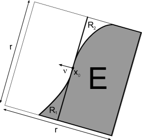
Figure 2: The sets E (in grey), $R_{1}$, and $R_{2}$.

For the reader’s convenience we end the section with a summary of standard measure-theoretic results used in the remainder. A key concept used in the development of the Liminf Inequality in Section 5 is that of a reduced boundary of the set $E:=\{x\in\Omega:v(x)=1\}$ associated to $v\in BV(\Omega;\{-1,1\})$. We recall that $v\in L^{1}(\Omega)$ is said to be of bounded variation, $v\in BV(\Omega)$, if the generalized partial derivatives $D_{i}$ of $v$ in the sense of distributions are bounded Radon measures. In particular $BV(\Omega;\{-1,1\})$ denotes functions of bounded variation taking values in the set $\{-1,1\}$, and $\text{Per}_{\Omega}(E):=|D\chi_{E}|(\Omega)<\infty$.

For sets of finite perimeter the reduced boundary $\partial^{*}E$ of $E$ is defined as the set of points $x_{0}\in\text{spt}|D\chi_{E}|\cap\Omega$ such that the limit

$$\nu(x_{0}):=-\lim_{r\rightarrow 0^{+}}\frac{D\chi_{E}(B_{r}(x_{0}))}{|D\chi_{E}|(B_{r}(x_{0}))}$$

exists and satisfies $|\nu(x_{0})|=1$. Here $B_{r}(x_{0})$ is the open ball of radius $r$ centered at $x_{0}$. For $x_{0}\in\partial^{*}E$ the vector $\nu(x_{0})$ is called the generalized outer unit normal to $E$. In particular, by Theorem 3.59 from [1], $|D\chi_{E}|=\mathcal{H}^{d-1}\mathbin{\vrule height=6.88889pt,depth=0.0pt,width=0.55974pt\vrule height=0.55974pt,depth=0.0pt,width=5.59721pt}\partial^{*}E$, and for $x_{0}\in\partial^{*}E$,

$$\lim_{r\rightarrow 0^{+}}\frac{\mathcal{H}^{d-1}(Q_{\nu}(x_{0},r)\cap\partial^{*}E)}{r^{d-1}}=1,$$

$$\lim_{r\rightarrow 0}\frac{1}{r^{d}}|R_{1}|=0,\quad\lim_{r\rightarrow 0}\frac{1}{r^{d}}|R_{2}|=0,$$ (2.12)

where

$$R_{1}:=\{x\in Q_{\nu}(x_{0},r)\cap E:(x-x_{0})\cdot\nu(x_{0})>0\},$$ (2.13)

$$R_{2}:=\{x\in Q_{\nu}(x_{0},r)\backslash E:(x-x_{0})\cdot\nu(x_{0})<0\},$$ (2.14)

and $|\cdot|$ denotes the Lebesgue measure in $\mathbb{R}^{d}$.

3 Compactness

In this section we prove the compactness Theorem 2.8. We use the following interpolation inequality.

Proposition 3.1.

Let $A\subset\mathbb{R}^{d}$ be a bounded open set in $\mathbb{R}^{d}$. Assume, in addition, that either $A$ has a $C^{1}$ boundary or that $A$ can be written as the union of finitely many pairwise disjoint open rectangles and a set of Lebesgue measure zero. Then there exist a constant $q_{*}\in(0,1)$, independent of $A$, and $\varepsilon_{0}=\varepsilon_{0}(A,q_{*})>0$ such that

$$q_{*}\int_{A}\varepsilon|\nabla v|^{2}dx\leq\int_{A}\left(\frac{W(v)}{\varepsilon}+\varepsilon^{3}|\nabla^{2}v|^{2}\right)dx$$ (3.1)

for every $\varepsilon\in(0,\varepsilon_{0})$ and $v\in W^{2,2}(A)$.

Proof.

See Theorem 1.2 in [7]. ∎

For every open set $A\subset\Omega$, $v\in W^{3,2}(\Omega)$, and $\varepsilon>0$, define the functional

$$\mathcal{I}_{\varepsilon}[v;A]:=\int_{A}\left(\frac{1}{\varepsilon}W(v)+\varepsilon|\nabla v|^{2}+\varepsilon^{3}|\nabla^{2}v|^{2}+\varepsilon^{5}|\nabla\Delta v|^{2}\right)dx.$$

Remark 3.2.

We note that in the energy ${\mathcal{F}}_{\varepsilon}[v]$ the potential $W$ acts on $u$, which is related to $v$ through the condition $u=-\varepsilon^{2}\Delta v+v$, while in $\mathcal{I}_{\varepsilon}[v]$ the potential acts on $v$. Hence ${\mathcal{F}}_{\varepsilon}$ differs from the standard Cahn-Hilliard energies involving solely the potential $W(v)$. In addition, the second order term in ${\mathcal{F}}_{\varepsilon}[v]$ involves the Laplacian $\Delta v$, while the second order term in $\mathcal{I}_{\varepsilon}[v]$ involves the Hessian $\nabla^{2}v$.

Next, we prove a result that will be useful to bound the energy from below and to obtain compactness of energy bounded sequences (see Theorem 2.8).

Proposition 3.3.

Let $K_{w},C_{w},c_{w},q_{*},\varepsilon_{0}>0$ be the constants given in Hypotheses 2.2 and Proposition 3.1. Then there exist $q_{0}>0$, depending only on $K_{w},C_{w},q_{*}$ (see (3.6)), and $\varepsilon_{1}>0$, depending only on $C_{w}$, such that for every $0<q\leq q_{0}$, $v\in W^{3,2}(\Omega)$, and $0<\varepsilon<\varepsilon_{1}$,

$${\mathcal{F}}_{\varepsilon}[v]\geq q\,\mathcal{I}_{\varepsilon}[v;\Omega]-\frac{12q}{q_{*}}C(\Omega)\varepsilon^{3}|\Omega|$$ (3.2)

for some constant $C(\Omega)>0$.

Proof.

If $v$ does not satisfy $\frac{\partial v}{\partial n}=0$ on $\partial\Omega$ then ${\mathcal{F}}_{\varepsilon}[v]=\infty$ and there is nothing to prove. Otherwise, fix $0<\theta\leq 1$. Using Taylor’s formula for $W$ and the fact that $W^{\prime\prime}$ is bounded by Hypotheses 2.2, yields

$${\mathcal{F}}_{\varepsilon}[v] ={\mathcal{F}}_{\varepsilon}[v;\Omega]=\int_{\Omega}\left(\frac{1}{\varepsilon}W(-\varepsilon^{2}\Delta v+v)-\varepsilon q|\nabla v|^{2}+(1-2q)\varepsilon^{3}(\Delta v)^{2}+(1-q)\varepsilon^{5}|\nabla\Delta v|^{2}\right)dx$$

$$\geq\int_{\Omega}\Big{(}\frac{\theta}{\varepsilon}W(v)-\theta W^{\prime}(v)\varepsilon\Delta v-\varepsilon q|\nabla v|^{2}+\Big{(}1-2q-\frac{\theta}{2}K_{w}\Big{)}\varepsilon^{3}(\Delta v)^{2}+(1-q)\varepsilon^{5}|\nabla\Delta v|^{2}\Big{)}dx.$$

By Young’s Inequality and the condition $|W^{\prime}(s)|\leq C_{w}\sqrt{W(s)}$ from Hypotheses 2.2, we have

$$W^{\prime}(v)\Delta v\leq\frac{1}{2\varepsilon^{2}C_{w}^{2}}(W^{\prime}(v))^{2}+\frac{\varepsilon^{2}}{2}C_{w}^{2}(\Delta v)^{2}\leq\frac{1}{2\varepsilon^{2}}W(v)+\frac{\varepsilon^{2}}{2}C_{w}^{2}(\Delta v)^{2}.$$ (3.4)

Substituting (3.4) into (3) implies

$${\mathcal{F}}_{\varepsilon}[v]\geq\int_{\Omega}\left(\frac{\theta}{2\varepsilon}W(v)-\varepsilon q|\nabla v|^{2}+\left(1-2q-\frac{\theta}{2}K_{w}-\frac{\theta}{2}C_{w}^{2}\right)\varepsilon^{3}(\Delta v)^{2}+(1-q)\varepsilon^{5}|\nabla\Delta v|^{2}\right)dx.$$

Multiplying (3.1), with $A=\Omega$, by $2q/q_{*}$ and using it in the previous inequality gives

$${\mathcal{F}}_{\varepsilon}[v] \geq\int_{\Omega}\Bigg{(}\left(\frac{\theta}{2}-\frac{2q}{q_{*}}\right)\frac{1}{\varepsilon}W(v)+\varepsilon q|\nabla v|^{2}+\left(1-2q-\frac{\theta}{2}K_{w}-\frac{\theta}{2}C_{w}^{2}\right)\varepsilon^{3}(\Delta v)^{2}$$

$$-\frac{2q\varepsilon^{3}}{q_{*}}|\nabla^{2}v|^{2}+(1-q)\varepsilon^{5}|\nabla\Delta v|^{2}\Bigg{)}dx.$$ (3.5)

Fix $\delta>0$. Using Proposition 2.11 we get

$${\mathcal{F}}_{\varepsilon}[v] \geq\int_{\Omega}\Bigg{(}\left(\frac{\theta}{2}-\frac{2q}{q_{*}}\right)\frac{1}{\varepsilon}W(v)-\left(\delta+\frac{2q}{q_{*}}\right)\varepsilon^{3}C(\Omega)v^{2}+\varepsilon q|\nabla v|^{2}$$

$$+\left(1-2q-\frac{\theta}{2}K_{w}-\frac{\theta}{2}C_{w}^{2}-\frac{6q}{q_{*}}-3\delta\right)\varepsilon^{3}(\Delta v)^{2}+\delta\varepsilon^{3}|\nabla^{2}v|^{2}+(1-q)\varepsilon^{5}|\nabla\Delta v|^{2}\Bigg{)}.$$

Finally, it follows from Hypotheses 2.2 that $W(s)\geq(c_{w}/4)s^{2}$ for $|s|\geq 2$. Hence

$${\mathcal{F}}_{\varepsilon}[v] \geq\int_{\Omega}\Bigg{(}\left[\frac{\theta}{2}-\frac{2q}{q_{*}}-\varepsilon^{4}\frac{4C(\Omega)}{c_{w}}\left(\delta+\frac{2q}{q_{*}}\right)\right]\frac{1}{\varepsilon}W(v)+\left(1-2q-\frac{\theta}{2}K_{w}-\frac{\theta}{2}C_{w}^{2}-\frac{6q}{q_{*}}-3\delta\right)\varepsilon^{3}(\Delta v)^{2}$$

$$+\varepsilon q|\nabla v|^{2}+\delta\varepsilon^{3}|\nabla^{2}v|^{2}+(1-q)\varepsilon^{5}|\nabla\Delta v|^{2}\Bigg{)}dx-4\left(\delta+\frac{2q}{q_{*}}\right)\varepsilon^{3}C(\Omega)|\Omega|.$$

Choosing $\delta:=\frac{q}{q_{*}}$, $\theta:=\frac{8q}{q_{*}}$, $\varepsilon_{1}:=\min\left\{\varepsilon_{0},\left(\frac{c_{w}}{12C(\Omega)}\right)^{1/4}\right\}$ and

$$q_{0}:=\frac{q_{*}}{2q_{*}+4K_{w}+4C_{w}^{2}+10}$$ (3.6)

yields (3.2). ∎

We now prove that for $q$ sufficiently small the “cell” energy is positive.

Proposition 3.4.

Let $m_{d}$ be defined in (2.2) and let $q_{0}$ be as in Proposition 3.3. Then $m_{d}>0$ for every $0<q<q_{0}.$

Proof.

Without loss of generality we may assume that the infimum in the definition of $m_{d}$ is taken over $0<\varepsilon<\varepsilon_{0}$. The result of the proposition then follows if we show that

$$\inf\left\{\int_{Q}\left(\frac{W(v)}{\varepsilon}+\varepsilon|\nabla v|^{2}\right)dx:0<\varepsilon<\varepsilon_{0},v\in{\mathcal{A}}\right\}>0.$$ (3.7)

Indeed, let $v\in{\mathcal{A}}$. Since $v$ satisfies periodic boundary conditions on $Q$, integration by parts yields

$$||\nabla^{2}v||_{L^{2}(Q)}^{2}=||\Delta v||_{L^{2}(Q)}^{2}.$$ (3.8)

Repeating the proof of Proposition 3.3 with $Q$ instead of $\Omega$ and using (3.8) in (3), we obtain

$${\mathcal{F}}_{\varepsilon}[v;Q]\geq q\,\mathcal{I}_{\varepsilon}[v;Q]\geq q\int_{Q}\left(\frac{W(v)}{\varepsilon}+\varepsilon|\nabla v|^{2}\right)dx$$

if $q\leq q_{0}$. To prove (3.7) we follow [13]. In particular, for $v\in{\mathcal{A}}$,

$$\int_{Q}\left(\frac{W(v)}{\varepsilon}+\varepsilon|\nabla v|^{2}\right)dx\geq 2\int_{Q}\sqrt{W(v)}|\nabla v|dx\geq\int_{Q^{\prime}}\int_{-1/2}^{1/2}\sqrt{W(v)}\left|\frac{\partial v}{\partial x_{d}}\right|dx_{d}dx^{\prime},$$ (3.9)

where $Q^{\prime}:=(-1/2,1/2)^{d-1}$. Since $v(x^{\prime},\pm 1/2)=\pm 1$ a change of variables yields

$$\int_{Q^{\prime}}\int_{-1/2}^{1/2}\sqrt{W(v)}\left|\frac{\partial v}{\partial x_{d}}\right|dx_{d}\,dx^{\prime}\geq\int_{-1}^{1}\sqrt{W(s)}\,ds.$$

Using this lower bound in (3.9) and taking the infimum over $v\in{\mathcal{A}}$ and $0<\varepsilon<\varepsilon_{0}$ gives (3.7). ∎

Proof of Theorem 2.8.

By Proposition 3.3 and (2.4)

$$\sup_{n}\ \mathcal{I}_{\varepsilon_{n}}[v_{n};\Omega]<\infty.$$ (3.10)

Hence, the Modica-Mortola energy, ${\mathcal{A}}_{\varepsilon}[v_{n}]$, of $v_{n}$ defined in (1.1) is uniformly bounded from above. The existence of some $v\in BV(\Omega;\{-1,1\})$ and a subsequence $\{v_{n_{k}}\}$ converging to $v$ in $L^{1}(\Omega)$ is well established for sequences of functions with uniformly bounded Modica-Mortola energy (see [27]).

To show the convergence in $L^{2}(\Omega)$, we recall again that by Hypotheses 2.2, $W(s)\geq(c_{w}/4)|s|^{2}$ for $|s|\geq 2$, and hence for every measurable set $E\subset\Omega$,

$$\int_{E}|v_{n}|^{2}\ dx =\int_{\{y\in E:|v_{n}(y)|<2\}}|v_{n}|^{2}dx+\int_{\{y\in E:|v_{n}(y)|\geq 2\}}|v_{n}|^{2}dx$$

$$\leq 4|E|+\frac{4}{c_{w}}\int_{E}W(v_{n})\leq 4|E|+C(q)\varepsilon_{n},$$

where in the last step we used (3.10). Therefore $\{|v_{n_{k}}|^{2}\}$ is equi-integrable, and convergence of $\{v_{n_{k}}\}$ to $v$ in $L^{2}(\Omega)$ is a consequence of Vitali’s Convergence Theorem.

To prove (2.5)₂, note that (3.10) implies $\varepsilon_{n}^{2}\|\Delta v_{n}\|_{L^{2}(\Omega)}\leq C(q)\varepsilon_{n}^{1/2}$. It follows that $\varepsilon_{n}^{2}\Delta v_{n}\rightarrow 0$ in $L^{2}(\Omega)$. ∎

4 Slicing Propositions

The slicing arguments in the following propositions will be used in the proof of the Liminf Inequality. In what follows we adopt the notation introduced in Definition 2.5.

Proposition 4.1.

There exists a constant $C(d)>0$ with the following property: If $K>0$, $k\in\mathbb{N}$, and $v\in W^{3,2}(Q(x_{0},r_{0}))$ are such that

$$\mathcal{I}_{\varepsilon}[v;Q(x_{0},r_{0})]\leq K$$ (4.1)

for some $0<\varepsilon<\varepsilon_{1}:=\frac{r_{0}}{4k\sqrt{C(d)}}$, then there exists $i\in\{1,\dots,k\}$ (depending on $v$) such that

$${\mathcal{F}}_{\varepsilon}[v;Q(x_{0},r)]\geq q\,\mathcal{I}_{\varepsilon}[v;Q(x_{0},r)]-\frac{q}{q_{*}}\frac{6K}{k}$$

and

$$\mathcal{I}_{\varepsilon}[v;L]\leq\frac{K}{k},$$

for all $r\in\left(\frac{r_{0}}{2}\left(1+\frac{2i-1}{2k}\right),\frac{r_{0}}{2}\left(1+\frac{i}{k}\right)\right)$ and all $0<q<q_{1}$, where

$$L:=Q\left(x_{0},\frac{r_{0}}{2}\left(1+\frac{i}{k}\right)\right)\backslash Q\left(x_{0},\frac{r_{0}}{2}\left(1+\frac{i-1}{k}\right)\right)$$

and

$$q_{1}:=\frac{q_{*}}{2q_{*}+4K_{w}+4C_{w}^{2}+3C(d)+1}.$$

Proof.

For simplicity we will use the notation $Q(r):=Q(x_{0},r)$. The following estimate is obtained from the proof of Lemma 9.2.3 in [19]. Let $0<r_{1}<r_{2}<r_{0}$. Then,

$$\int_{Q(r_{1})}|\nabla^{2}v|^{2}\leq C(d)\left(\int_{Q(r_{2})}|\Delta v|^{2}\ dx+\frac{1}{(r_{2}-r_{1})^{2}}\int_{Q(r_{2})\backslash Q(r_{1})}|\nabla v|^{2}\ dx\right).$$ (4.2)

Given $k\in\mathbb{N}$, we first partition the set $Q(r_{0})\backslash Q(r_{0}/2)$ into $k$ layers

$$L^{i}:=Q\left(\frac{r_{0}}{2}\left(1+\frac{i}{k}\right)\right)\setminus Q\left(\frac{r_{0}}{2}\left(1+\frac{i-1}{k}\right)\right),\quad i=1,\dots,k.$$

Since

$$\sum_{i=1}^{k}\mathcal{I}_{\varepsilon}[v;L^{i}]\leq\mathcal{I}_{\varepsilon}[v;Q(r_{0})],$$

by (4.1) there exists a layer $L^{i^{*}}$ satisfying

$$\mathcal{I}_{\varepsilon}[v;L^{i^{*}}]\leq\frac{1}{k}\mathcal{I}_{\varepsilon}[v;Q(r_{0})]\leq\frac{K}{k}.$$ (4.3)

Fix $r\in\left(\frac{r_{0}}{2}\left(1+\frac{2i^{*}-1}{2k}\right),\frac{r_{0}}{2}\left(1+\frac{i^{*}}{k}\right)\right)$. Choosing $r_{1}:=\frac{r_{0}}{2}\left(1+\frac{i^{*}-1}{k}\right)$, $r_{2}:=r$ and applying estimate (4.2) we obtain

$$\int_{Q(r_{1})}|\nabla^{2}v|^{2}\ dx\leq C(d)\ \left(\int_{Q(r)}|\Delta v|^{2}\ dx+\frac{16k^{2}}{r_{0}^{2}}\int_{L^{i^{*}}}|\nabla v|^{2}\ dx\right).$$

Adding $\int_{L^{i^{*}}}|\nabla^{2}v|^{2}\ dx$ to both sides and multiplying by $\varepsilon^{3}$ yields, by (4.3),

$$\varepsilon^{3}\int_{Q(r)}|\nabla^{2}v|^{2}\ dx \leq C(d)\ \left(\varepsilon^{3}\int_{Q(r)}|\Delta v|^{2}\ dx+\frac{16k^{2}}{r_{0}^{2}}\varepsilon^{3}\int_{L^{i^{*}}}|\nabla v|^{2}\ dx\right)+\varepsilon^{3}\int_{L^{i^{*}}}|\nabla^{2}v|^{2}\ dx$$

$$\leq C(d)\left(\varepsilon^{3}\int_{Q(r)}|\Delta v|^{2}\ dx+\frac{16k^{2}}{r_{0}^{2}}\varepsilon^{2}\frac{K}{k}\right)+\frac{K}{k}.$$

Let $0<\varepsilon_{1}^{2}=\frac{r_{0}^{2}}{16k^{2}C(d)}$. Then for $0<\varepsilon<\varepsilon_{1}$ we have

$$\varepsilon^{3}\int_{Q(r)}|\nabla^{2}v|^{2}\ dx\leq C(d)\ \varepsilon^{3}\int_{Q(r)}|\Delta v|^{2}\ dx+\frac{2K}{k}.$$ (4.4)

Repeating the argument of the proof of Proposition 3.3 with $\theta:=\frac{8q}{q_{*}}$ until (3) and using (4.4) multiplied by 3 in place of Proposition 2.11 yields

$${\mathcal{F}}_{\varepsilon}[v;Q(r)] \geq\int_{Q(r)}\Bigg{(}\frac{2q}{q_{*}}\frac{1}{\varepsilon}W(v)+\left(1-2q-\frac{4q}{q_{*}}K_{w}-\frac{4q}{q_{*}}C_{w}^{2}-\frac{3q}{q_{*}}C(d)\right)\varepsilon^{3}|\Delta v|^{2}$$

$$+q\varepsilon|\nabla v|^{2}+\frac{q}{q_{*}}\varepsilon^{3}|\nabla^{2}v|^{2}+(1-q)\varepsilon^{5}|\nabla\Delta v|^{2}\Bigg{)}dx-\frac{q}{q_{*}}\frac{6K}{k}$$

$$\geq q\,\mathcal{I}_{\varepsilon}[v;Q(r)]-\frac{q}{q_{*}}\frac{6K}{k},$$

provided $0<q<q_{1}$. This completes the proof. ∎

Proposition 4.2.

Let $k\in\mathbb{N}$, $\varepsilon_{n}\rightarrow 0^{+}$, $\nu\in\mathbb{S}^{d-1}$, and $\{w_{n}\}\subset W^{3,2}(Q_{\nu}(0,1))$ be such that

$$\lim_{n\rightarrow\infty}\int_{Q_{\nu}(0,1)}|w_{n}-v_{0}|^{2}dx=0,$$

and

$$\mathcal{I}_{\varepsilon_{n}}[w_{n};\tilde{L}_{k}]\leq\frac{C_{0}}{k}$$ (4.5)

for all $n$ and some $C_{0}>0$, not dependent on $k$, where

$$v_{0}(y):=\left\{\begin{array}[]{ll}1&\mbox{ if }y\cdot\nu<0,\\ -1&\mbox{ if }y\cdot\nu>0,\end{array}\right.$$

and

$$\tilde{L}_{k}:=Q_{\nu}(0,1)\backslash Q_{\nu}(0,1-1/(4k)).$$

Then

$${\mathcal{F}}_{\varepsilon_{n}}[w_{n};Q_{\nu}(0,1)]\geq m_{d}-\frac{C}{k},$$

where the constant $C$ does not depend on $k$.

Proof.

We modify $\{w_{n}\}$ to belong to the admissible class ${\mathcal{A}}_{\nu}$ without increasing the energy. Given $\Psi\in C_{c}^{\infty}(\mathbb{R}^{d})$, with $\mbox{supp}(\Psi)\subset B_{1}(0)$ and $\int_{\mathbb{R}^{d}}\Psi(y)dy=1$, and $\varepsilon>0$, consider the mollifier

$$\Psi_{\varepsilon}(y):=\frac{1}{\varepsilon^{d}}\Psi\left(\frac{y}{\varepsilon}\right)$$ (4.6)

and

$$\varphi_{n}:=v_{0}\ast\Psi_{\varepsilon_{n}}.$$

Note that $\varphi_{n}\in C^{\infty}(\mathbb{R}^{d})$ and

$$||\varphi_{n}||_{L^{\infty}(\mathbb{R^{d}})}\leq 1,\quad||\nabla\varphi_{n}||_{L^{\infty}(\mathbb{R^{d}})}\leq C\varepsilon_{n}^{-1},\quad||\nabla^{2}\varphi_{n}||_{L^{\infty}(\mathbb{R^{d}})}\leq C\varepsilon_{n}^{-2},\quad||\nabla^{3}\varphi_{n}||_{L^{\infty}(\mathbb{R^{d}})}\leq C\varepsilon_{n}^{-3}.$$ (4.7)

In addition,

$$\varphi_{n}(y)=\left\{\begin{array}[]{ll}1&\mbox{ if }y\cdot\nu<-\varepsilon_{n},\\ -1&\mbox{ if }y\cdot\nu>\varepsilon_{n},\end{array}\right.$$

and

$$\nabla^{s}\varphi_{n}(y)=0\mbox{ if }|y\cdot\nu|>\varepsilon_{n},\quad s=1,2,3.$$

Hence for $\varepsilon_{n}$ sufficiently small $\varphi_{n}\in{\mathcal{A}}_{\nu}$. We want to define a function $z_{n}$ to equal $\varphi_{n}$ near the boundary of $Q_{\nu}$ and $w_{n}$ away from the boundary. To be precise, we first partition the set $\tilde{L}_{k}=Q_{\nu}(0,1)\backslash Q_{\nu}(0,1-1/(4k))$ into $\lceil\varepsilon_{n}^{-1}\rceil$ layers,

$$L_{n}^{i}:=Q_{\nu}\left(0,1-\frac{i-1}{4k\lceil\varepsilon_{n}^{-1}\rceil}\right)\Big{\backslash}Q_{\nu}\left(0,1-\frac{i}{4k\lceil\varepsilon_{n}^{-1}\rceil}\right),\quad i=1,\dots,\lceil\varepsilon_{n}^{-1}\rceil,$$

where $\lceil x\rceil$ is defined as the smallest integer not less than $x$. Since both $w_{n}\rightarrow v_{0}$ in $L^{2}(Q_{\nu})$ and $\varphi_{n}\rightarrow v_{0}$ in $L^{2}(Q_{\nu})$, we have

$$||w_{n}-\varphi_{n}||_{L^{2}(Q_{\nu})}^{2}\rightarrow 0\mbox{ as }n\rightarrow\infty.$$

Note that $\cup_{i}L_{n}^{i}=\tilde{L}_{k}\subset Q_{\nu}(0,1)$ and that $L_{n}^{i}$ are pairwise disjoint, so the sum over all of the layers is bounded by

$$\sum_{i}\mathcal{I}_{\varepsilon_{n}}[w_{n};L_{n}^{i}]+\frac{\sum_{i}||w_{n}-\varphi_{n}||_{L^{2}(L_{n}^{i})}^{2}}{||w_{n}-\varphi_{n}||_{L^{2}(Q_{\nu})}^{2}}\leq\frac{C_{0}}{k}+1.$$

Since there are $\lceil\varepsilon_{n}^{-1}\rceil$ layers, for one of these layers, say $L_{n}:=L_{n}^{i^{*}}$, it holds

$$\mathcal{I}_{\varepsilon_{n}}[w_{n};L_{n}]+\frac{||w_{n}-\varphi_{n}||_{L^{2}(L_{n})}^{2}}{||w_{n}-\varphi_{n}||_{L^{2}(Q_{\nu})}^{2}}\leq\left(\frac{C_{0}}{k}+1\right)\,\varepsilon_{n}.$$ (4.8)

Define

$$z_{n}:=\eta_{n}{w}_{n}+(1-\eta_{n})\varphi_{n},$$

where $\eta_{n}$ is a smooth function with support in $Q_{\nu}(0,1)$ such that

$$\eta_{n}(x):=\left\{\begin{array}[]{ll}0&\mbox{ if }x\in Q_{n}^{out}:=Q_{\nu}\left(0,1\right)\backslash Q_{\nu}\left(0,1-\frac{i^{*}-1}{4k\lceil\varepsilon_{n}^{-1}\rceil}\right),\\ \in(0,1)&\mbox{ if }x\in L_{n},\\ 1&\mbox{ if }x\in Q_{n}^{in}:=Q_{\nu}\backslash(Q_{n}^{out}\cup L_{n}),\end{array}\right.$$

and

$$||\nabla^{s}\eta_{n}||_{L^{\infty}(Q_{\nu})}=\mathcal{O}\left(\frac{k^{s}}{\varepsilon_{n}^{s}}\right),\quad s=1,2,3.$$ (4.9)

Moreover,

$${\mathcal{F}}_{\varepsilon_{n}}[z_{n};Q_{\nu}]={\mathcal{F}}_{\varepsilon_{n}}[\varphi_{n};Q_{n}^{out}]+{\mathcal{F}}_{\varepsilon_{n}}[z_{n};L_{n}]+{\mathcal{F}}_{\varepsilon_{n}}[w_{n};Q_{n}^{in}].$$

We observe that since ${\mathcal{F}}_{\varepsilon_{n}}[w_{n};Q_{\nu}\backslash Q_{n}^{in}]$ can be negative it is not necessarily true that ${\mathcal{F}}_{\varepsilon_{n}}[w_{n};Q_{n}^{in}]\leq{\mathcal{F}}_{\varepsilon_{n}}[w_{n};Q_{\nu}].$ Instead, we use (4.5) to control the negative terms to obtain

$${\mathcal{F}}_{\varepsilon_{n}}[z_{n};Q_{\nu}] \leq{\mathcal{F}}_{\varepsilon_{n}}[\varphi_{n};Q_{n}^{out}]+{\mathcal{F}}_{\varepsilon_{n}}[z_{n};L_{n}]+{\mathcal{F}}_{\varepsilon_{n}}[w_{n};Q_{\nu}]+q\int_{L}\varepsilon_{n}|\nabla w_{n}|^{2}dx$$

$$\leq{\mathcal{F}}_{\varepsilon_{n}}[\varphi_{n};Q_{n}^{out}]+{\mathcal{F}}_{\varepsilon_{n}}[z_{n};L_{n}]+{\mathcal{F}}_{\varepsilon_{n}}[w_{n};Q_{\nu}]+q\frac{C_{0}}{k}.$$ (4.10)

Note that for $s=1,2,3$,

$$\varepsilon_{n}^{2s-1}\int_{Q_{n}^{out}}|\nabla^{s}\varphi_{n}|^{2}dx\leq\varepsilon_{n}^{2s-1}\frac{C}{\varepsilon_{n}^{2s}}|\{x\in Q_{n}^{out}:\varphi_{n}\neq\pm 1\}|\leq\frac{C}{k}.$$ (4.11)

In addition, by the continuity of $W$,

$$\frac{1}{\varepsilon_{n}}\int_{Q_{n}^{out}}W(-\varepsilon_{n}^{2}\Delta\varphi_{n}+\varphi_{n})dx\leq\frac{C}{\varepsilon_{n}}|\{x\in Q_{n}^{out}:\varphi_{n}\neq\pm 1\}|\leq\frac{C}{k}.$$ (4.12)

Together (4.11) and (4.12) imply

$${\mathcal{F}}_{\varepsilon_{n}}[\varphi_{n};Q_{n}^{out}]\leq\frac{C}{k}.$$ (4.13)

To estimate ${\mathcal{F}}_{\varepsilon_{n}}[z_{n};L_{n}]$, we first note that

$$\partial_{x_{i}}z_{n}=\partial_{x_{i}}\eta_{n}(w_{n}-\varphi_{n})+\eta_{n}\partial_{x_{i}}w_{n}+(1-\eta_{n})\partial_{x_{i}}\varphi_{n},$$

and

$$\partial_{x_{i}x_{k}}z_{n} =\partial_{x_{i}x_{k}}\eta_{n}(w_{n}-\varphi_{n})+\partial_{x_{i}}\eta_{n}\partial_{x_{k}}w_{n}+\partial_{x_{k}}\eta_{n}\partial_{x_{i}}w_{n}+\eta_{n}\partial_{x_{i}x_{k}}w_{n}$$

$$-\partial_{x_{i}}\eta_{n}\partial_{x_{k}}\varphi_{n}-\partial_{x_{k}}\eta_{n}\partial_{x_{i}}\varphi_{n}+(1-\eta_{n})\partial_{x_{i}x_{k}}\varphi_{n}.$$

We use (4.8) to control the derivatives of $w_{n}$ in the transition region $L_{n}$. From (4.7), (4.8), (4.9), the expressions for the derivatives of $z_{n}$ and the fact that $||w_{n}-\varphi_{n}||_{L^{2}(Q)}\rightarrow 0$, we readily obtain the following bounds on the terms in ${\mathcal{F}}_{\varepsilon_{n}}[z_{n};L_{n}]$,

$$\varepsilon_{n}\int_{L_{n}}|\nabla z_{n}|^{2}dx \leq C\int_{L_{n}}\left(\varepsilon_{n}|\nabla\eta_{n}|^{2}|w_{n}-\varphi_{n}|^{2}+\varepsilon_{n}\eta_{n}^{2}|\nabla w_{n}|^{2}+\varepsilon_{n}(1-\eta_{n})^{2}|\nabla\varphi_{n}|^{2}\right)dx$$

$$\leq C\left(\frac{k^{2}\varepsilon_{n}}{\varepsilon_{n}^{2}}||w_{n}-\varphi_{n}||_{L^{2}(L_{n})}^{2}+\left(\frac{C_{0}}{k}+1\right)\varepsilon_{n}+\frac{\varepsilon_{n}}{\varepsilon_{n}^{2}}|\{x\in L_{n}:\varphi_{n}\neq\pm 1\}|\right)$$

$$\leq C\left(k^{2}\left(\frac{C_{0}}{k}+1\right)||w_{n}-\varphi_{n}||_{L^{2}(L)}^{2}+\left(\frac{C_{0}}{k}+1\right)\varepsilon_{n}+\frac{\varepsilon_{n}}{k}\right)\leq\frac{C}{k}$$ (4.14)

for $n$ sufficiently large, where we used $\left|\{x\in L_{n}:|x\cdot\nu|<\varepsilon_{n}\}\right|=\mathcal{O}(\varepsilon_{n}^{2}/k)$. Similarly,

$$\varepsilon_{n}^{3}\int_{L_{n}}|\nabla^{2}z_{n}|dx \leq C\varepsilon_{n}^{3}\int_{L_{n}}\Big{(}|\nabla^{2}\eta_{n}|^{2}|w_{n}-\varphi_{n}|^{2}+2|\nabla\eta_{n}|^{2}|\nabla w_{n}|^{2}+2|\nabla\eta_{n}|^{2}|\nabla\varphi_{n}|^{2}+\eta_{n}^{2}|\nabla^{2}w_{n}|^{2}$$

$$+(1-\eta_{n})^{2}|\nabla^{2}\varphi_{n}|^{2}\Big{)}dx\leq C\Bigg{(}\frac{\varepsilon_{n}^{3}k^{4}}{\varepsilon_{n}^{4}}\left(\frac{C_{0}}{k}+1\right)\varepsilon_{n}||w_{n}-\varphi_{n}||_{L^{2}(L)}^{2}+\frac{\varepsilon_{n}^{2}k^{2}}{\varepsilon_{n}^{2}}\left(\frac{C_{0}}{k}+1\right)\varepsilon_{n}$$

$$+\varepsilon_{n}^{3}\left(\frac{k^{2}}{\varepsilon_{n}^{2}}\frac{1}{\varepsilon_{n}^{2}}+\frac{1}{\varepsilon_{n}^{4}}\right)|\{x\in L_{n}:\varphi_{n}\neq\pm 1\}|+\left(\frac{C_{0}}{k}+1\right)\varepsilon_{n}\Bigg{)}\leq\frac{C}{k}$$

for $n$ sufficiently large. To bound the integral involving the potential $W$ we first remark that by Hypotheses 2.2 (and Remark 2.3) $W$ grows quadratically at infinity. Splitting the integral into regions where $|-\varepsilon_{n}^{2}\Delta z_{n}+z_{n}|\leq 2$ and $|-\varepsilon_{n}^{2}\Delta z_{n}+z_{n}|>2$, we use the quadratic growth of $W$ to obtain,

$$\left|\frac{1}{\varepsilon_{n}}\int_{L_{n}}W(-\varepsilon_{n}^{2}\Delta z_{n}+z_{n})dx\right|\leq\frac{\sup_{|s|\leq 2}W(s)}{\varepsilon_{n}}|L_{n}|+\frac{C_{w}^{2}}{4\varepsilon_{n}}\int_{L_{n}}(-\varepsilon_{n}^{2}\Delta z_{n}+z_{n})^{2}dx$$

$$\leq\frac{C}{k}+\frac{C_{w}^{2}}{2}\int_{L_{n}}\varepsilon_{n}^{3}|\Delta z_{n}|^{2}dx+\frac{C_{w}^{2}}{2\varepsilon_{n}}\int_{L_{n}}z_{n}^{2}dx\leq\frac{C}{k}+\frac{C_{w}^{2}}{2}\int_{L_{n}}\varepsilon_{n}^{3}|\Delta z_{n}|^{2}dx+\frac{C_{w}^{2}}{\varepsilon_{n}}\int_{L_{n}}(w_{n}^{2}+\varphi_{n}^{2})dx$$

$$\leq\frac{C}{k}+\frac{C_{w}^{2}}{2}\int_{L_{n}}\varepsilon_{n}^{3}|\Delta z_{n}|^{2}dx+\frac{C}{\varepsilon_{n}}\int_{L_{n}}W(w_{n})dx+\frac{C}{\varepsilon_{n}}|L_{n}|\leq\left(\frac{C_{0}}{k}+1\right)\varepsilon_{n}+\frac{C}{k}\leq\frac{C}{k}$$ (4.15)

for $n$ sufficiently large, where we again used (4.8). Analogous calculations are used to estimate
$\varepsilon_{n}^{5}\int_{L_{n}}|\nabla\Delta z_{n}|^{2}dx$. Combining estimates (4.13), (4.2)-(4.2) with (4.2) completes the proof. ∎

5 Proof of the Liminf Inequality

In this section we prove the Liminf Inequality of Theorem 2.9. We use the blow-up method to reduce the problem to a unit cube, where we follow the general lines of [7]. In what follows we assume $q\leq\min\{q_{0},q_{1}\}$ (see Propositions 3.3 and 4.1). Fix $\varepsilon_{n}\rightarrow 0^{+}$ and $\{v_{n}\}\subset W^{3,2}(\Omega)$, $v_{n}\rightarrow v\in L^{2}(\Omega)$. We may assume that

$$\liminf_{n\rightarrow\infty}{\mathcal{F}}_{\varepsilon_{n}}[v_{n}]<\infty,$$ (5.1)

and we extract a subsequence $\{v_{n_{k}}\}$ of $\{v_{n}\}$ satisfying

$$\lim_{k\rightarrow\infty}{\mathcal{F}}_{\varepsilon_{n_{k}}}[v_{n_{k}}]=\liminf_{n\rightarrow\infty}{\mathcal{F}}_{\varepsilon_{n}}[v_{n}]<\infty.$$

By selecting a further subsequence, if necessary, we can assume that $\sup_{k}{\mathcal{F}}_{\varepsilon_{n_{k}}}[v_{n_{k}}]<\infty$ so that by Proposition 3.3,

$$\sup_{k}\mathcal{I}_{\varepsilon_{n_{k}}}[v_{n_{k}};\Omega]=:K<\infty.$$ (5.2)

Since $v_{n_{k}}\rightarrow v$ in $L^{2}(\Omega)$, Theorem 2.8 implies that $v\in BV(\Omega;\{-1,1\})$. Therefore,

$$v=\chi_{E}-\chi_{\Omega\backslash E},$$ (5.3)

where $\mbox{Per}_{\Omega}(E)<\infty$. In what follows, to simplify notation we denote the subsequence of $\{v_{n}\}$ extracted in (5.2) by $\{v_{n}\}$.

We first note that, due to (5.1) and (5.2), the sequences of functions

$$f_{n}:=\frac{1}{\varepsilon_{n}}W(-\varepsilon_{n}^{2}\Delta v_{n}+v_{n})-\varepsilon_{n}q|\nabla v_{n}|^{2}+(1-2q)\varepsilon_{n}^{3}|\Delta v_{n}|^{2}+(1-q)\varepsilon_{n}^{5}|\nabla\Delta v_{n}|^{2}$$

and

$$g_{n}:=\frac{1}{\varepsilon_{n}}W(v_{n})+\varepsilon_{n}|\nabla v_{n}|^{2}+\varepsilon_{n}^{3}|\Delta v_{n}|^{2}+\varepsilon_{n}^{5}|\nabla\Delta v_{n}|^{2}$$

are bounded in $L^{1}(\Omega)$. Consider the signed Radon measures defined on Borel subsets of $\Omega$,

$$\lambda_{n}(B):=\int_{B}f_{n}\ dx,\quad\zeta_{n}(B):=\int_{B}g_{n}\ dx.$$

Up to subsequences, not relabeled, we may assume that there exist Radon measures $\lambda$, $\mu$, $\zeta$ such that

$$\lambda_{n}\mbox{ }\rightharpoonup^{*}\lambda,\quad|\lambda_{n}|\rightharpoonup^{*}\mu,\quad\zeta_{n}\rightharpoonup^{*}\zeta$$

in the space $\mathcal{M}_{b}(\Omega)$ of all bounded signed Radon measures on $\Omega$ (see Proposition 1.202 in [12]), where $|\lambda_{n}|$ denotes the total variation of $\lambda_{n}$. We claim that $\lambda\geq 0$.

Suppose that $\lambda\neq 0$. By the Besicovitch Derivation Theorem (Theorem 1.155 in [12]), for $|\lambda|$-a.e. $x_{0}\in\Omega$

$$\frac{d\lambda}{d|\lambda|}(x_{0})=\lim_{r\rightarrow 0^{+}}\frac{\lambda(Q(x_{0},r))}{|\lambda|(Q(x_{0},r))}\in\mathbb{R},$$ (5.4)

where $|\lambda|$ is the total variation of $\lambda$. Fix any $x_{0}$ for which (5.4) holds and $|\lambda|(Q(x_{0},r))>0$ for all $r>0$ sufficiently small. Let $\eta\in(0,1)$ and find $\bar{r}_{\eta}>0$ such that

$$\frac{d\lambda}{d|\lambda|}(x_{0})\geq\frac{\lambda(Q(x_{0},r))}{|\lambda|(Q(x_{0},r))}-\eta$$ (5.5)

for all $0<r<\bar{r}_{\eta}$.

Fix $0<r_{0}<\bar{r}_{\eta}$ and $k\in\mathbb{N}$. By Proposition 4.1 for every $n$ there exists $i_{n}\in\{1,\dots,k\}$ such that

$${\mathcal{F}}_{\varepsilon_{n}}[v;Q(x_{0},r)]\geq q\mathcal{I}_{\varepsilon_{n}}[v;Q(x_{0},r)]-\frac{q}{q^{*}}\frac{6K}{k}$$ (5.6)

for all $r\in\left(\frac{r_{0}}{2}\left(1+\frac{2i_{n}-1}{2k}\right),\frac{r_{0}}{2}\left(1+\frac{i_{n}}{k}\right)\right)$ where $K$ is given in (5.2). Since $i_{n}\in\{1,\dots,k\}$ for all $n$, there exists $i^{(1)}\in\{1,\dots,k\}$ such that $i^{(1)}=i_{n}$ for infinitely many $n$, say $n_{l}$, $l\in\mathbb{N}$. Let $k$ be so large that

$$\frac{q}{q_{*}}\frac{6K}{k}\leq|\lambda|(Q(x_{0},r_{0}/2))\eta$$ (5.7)

and take

$$r_{1}\in\left(\frac{r_{0}}{2}\left(1+\frac{2i^{(1)}-1}{2k}\right),\frac{r_{0}}{2}\left(1+\frac{i^{(1)}}{k}\right)\right)$$

such that $\mu(\partial Q(x_{0},r_{1}))=0$. Then by (5.5), Corollary 1.204 in [12], (5.6), and (5.7)

$$\frac{d\lambda}{d|\lambda|}(x_{0}) \geq\frac{\lambda(Q(x_{0},r_{1}))}{|\lambda|(Q(x_{0},r_{1}))}-\eta=\lim_{n\rightarrow\infty}\frac{{\mathcal{F}}_{\varepsilon_{n_{l}}}[v_{n_{l}};Q(x_{0},r_{1})]}{|\lambda|(Q(x_{0},r_{0}))}-\eta$$

$$\geq\liminf_{n\rightarrow\infty}\frac{q\mathcal{I}_{\varepsilon_{n_{l}}}[v_{n_{l}};Q(x_{0},r_{1})]-|\lambda|(Q(x_{0},r_{0}/2)\eta}{|\lambda|(Q(x_{0},r_{1}))}-\eta$$

$$\geq-2\eta,$$

where we used the fact that $r_{0}/2<r_{1}$ so that $|\lambda|(Q(x_{0},r_{1}))\geq|\lambda|(Q(x_{0},r_{0}/2))$. Letting $\eta\rightarrow 0^{+}$ we conclude that $\frac{d\lambda}{d|\lambda|}(x_{0})\geq 0$.

This shows that $\lambda\geq 0$. In turn, by the Radon-Nikodym and Lebesgue Decomposition theorems ([12] Theorem 1.180) we can decompose

$$\lambda=\lambda_{ac}+\lambda_{s},$$

where $\lambda_{ac}\ll\xi$, $\lambda_{s}\geq 0$, $\lambda_{s}\perp\xi$, with

$$\xi(B):=\mathcal{H}^{d-1}(B\cap\partial^{*}E),\quad B\subset\Omega\mbox{ Borel}.$$

We claim that for $\mathcal{H}^{d-1}$-a.e. $x_{0}\in\Omega\cap\partial^{*}E$,

$$\frac{d\lambda_{ac}}{d\xi}(x_{0})\geq m_{d},$$ (5.8)

where $m_{d}$ is the constant defined in (2.2). Observe that if (5.8) holds, then, since $\lambda_{s}\geq 0$,

$$\lim_{n\rightarrow\infty}{\mathcal{F}}_{\varepsilon_{n}}[v_{n};\Omega] =\lim_{n\rightarrow\infty}\lambda_{n}(\Omega)\geq\lambda(\Omega)\geq\lambda_{ac}(\Omega)=\int_{\Omega}\frac{d\lambda_{ac}}{d\xi}d\xi$$

$$\geq m_{d}\mathcal{H}^{d-1}(\Omega\cap\partial^{*}E)=m_{d}\mbox{Per}_{\Omega}(E),$$

which gives (2.6) (see (2.3) and (5.3)). In the remainder of the proof we show (5.8).

To this end we first note that by the Besicovitch Derivation Theorem (Theorem 1.155 in [12]), for $\mathcal{H}^{d-1}$-a.e. $x_{0}\in\Omega\cap\partial^{*}E$

$$\infty>\frac{d\lambda_{ac}}{d\mathcal{H}^{d-1}}(x_{0})=\lim_{r\rightarrow 0^{+}}\frac{\lambda(Q_{\nu}(x_{0},r))}{\mathcal{H}^{d-1}(Q_{\nu}(x_{0},r)\cap\partial^{*}E)}=\lim_{r\rightarrow 0^{+}}\frac{\lambda(Q_{\nu}(x_{0},r))}{r^{d-1}},$$ (5.9)

$$\infty>\frac{d\zeta_{ac}}{d\mathcal{H}^{d-1}}(x_{0})=\lim_{r\rightarrow 0^{+}}\frac{\zeta(Q_{\nu}(x_{0},r))}{\mathcal{H}^{d-1}(Q_{\nu}(x_{0},r)\cap\partial^{*}E)}=\lim_{r\rightarrow 0^{+}}\frac{\zeta(Q_{\nu}(x_{0},r))}{r^{d-1}},$$ (5.10)

where $\nu$ denotes the outward normal vector to $E$ at $x_{0}$. Fix $x_{0}\in\Omega\cap\partial^{*}E$ for which (5.9) and (5.10) hold. Then there exists $\bar{r}>0$ such that

$$\frac{\zeta(Q_{\nu}(x_{0},r))}{r^{d-1}}\leq\frac{d\zeta_{ac}}{d\mathcal{H}^{d-1}}(x_{0})+1=:M$$

for all $0<r\leq\bar{r}$. Let $0<r_{0}\leq\bar{r}$ be such that $\zeta(\partial Q_{\nu}(x_{0},r_{0}))=\mu(\partial Q_{\nu}(x_{0},r_{0}))=0$. Then by Corollary 1.204 in [12],

$$\lim_{n\rightarrow\infty}\frac{\mathcal{I}_{\varepsilon_{n}}[v_{n};Q_{\nu}(x_{0},r_{0})]}{r_{0}^{d-1}}=\frac{\zeta(Q_{\nu}(x_{0},r_{0}))}{r_{0}^{d-1}}\leq M$$

and so

$$\mathcal{I}_{\varepsilon_{n}}[v_{n};Q_{\nu}(x_{0},r_{0})]\leq(M+1)\,r_{0}^{d-1}$$

for all $n\geq n_{0}=n_{0}(r_{0})$. Let $k\in\mathbb{N}$. By Proposition 4.1 with $K:=(M+1)r_{0}^{d+1}$, for each $n\geq n_{0}$ there exists $i_{n}\in\{1,\dots,k\}$ such that

$$\mathcal{I}_{\varepsilon_{n}}[v_{n};L_{i_{n}}]\leq\frac{(M+1)\,r_{0}^{d-1}}{k},$$

where $L_{i_{n}}:=Q_{\nu}\left(x_{0},\frac{r_{0}}{2}\left(1+\frac{i_{n}}{k}\right)\right)\backslash Q_{\nu}\left(x_{0},\frac{r_{0}}{2}\left(1+\frac{i_{n}-1}{k}\right)\right)$.

Since $i_{n}\in\{1,\dots,k\}$ for all $n\geq n_{0}$, there exists $i^{(1)}\in\{1,\dots,k\}$ such that $i^{(1)}=i_{n}$ for infinitely many $n$, say $n_{l}^{(1)},l\in\mathbb{N}$. Let $L^{(1)}:=L_{i^{(1)}}$. Then

$$\mathcal{I}_{\varepsilon_{n_{l}^{(1)}}}[v_{n_{l}^{(1)}};L^{(1)}]\leq\frac{(M+1)\,r_{0}^{d-1}}{k}$$

for all $n_{l}^{(1)}$, $l\in\mathbb{N}$. We proceed by induction. Let

$$\alpha_{k}:=\max\left\{\frac{4k(k+i-1)}{(4k-1)(k+i)}:\,i=1,\ldots k\right\}=1-\frac{1}{4k-1}.$$

Fix $\beta_{k}\in(\alpha_{k},1)$ and for $j\in\mathbb{N}$ choose

$$r_{j}\in\left(\frac{r_{j-1}}{2}\left(1+\frac{4i^{(j)}-3}{4k-1}\right),\beta_{k}\frac{r_{j-1}}{2}\left(1+\frac{i^{(j)}}{k}\right)\right)$$ (5.11)

such that $\zeta(\partial Q_{\nu}(x_{0},r_{j}))=\mu(\partial Q_{\nu}(x_{0},r_{j}))=0$. Note that $r_{j}\rightarrow 0^{+}$ since $r_{j}<\beta_{k}r_{j-1}$ for all $j$. Thus, for every $j$ we find a subsequence $\{v_{n_{l}^{(j)}}\}_{l\in\mathbb{N}}\subset\{v_{n_{l}^{(j-1)}}\}_{l\in\mathbb{N}}$ and a layer

$$L^{(j+1)}:=Q_{\nu}\left(x_{0},\frac{r_{j}}{2}\left(1+\frac{i^{(j+1)}}{k}\right)\right)\backslash Q_{\nu}\left(x_{0},\frac{r_{j}}{2}\left(1+\frac{i^{(j+1)}-1}{k}\right)\right)$$ (5.12)

such that

$$\mathcal{I}_{\varepsilon_{n_{l}^{(j+1)}}}[v_{n_{l}^{(j+1)}};L^{(j+1)}]\leq\frac{(M+1)\,r_{j}^{d-1}}{k}$$ (5.13)

for all $l\in\mathbb{N}$.

By (5.9) and Corollary 1.204 in [12],

$$\frac{d\lambda_{ac}}{d\mathcal{H}^{d-1}}(x_{0})=\lim_{j\rightarrow\infty}\frac{\lambda(Q_{\nu}(x_{0},r_{j}))}{r_{j}^{d-1}}=\lim_{j\rightarrow\infty}\lim_{n\rightarrow\infty}\frac{{\mathcal{F}}_{\varepsilon_{n}}[v_{n};Q_{\nu}(x_{0},r_{j})]}{r_{j}^{d-1}},$$

and by Theorem 3.59 from [1] (see also (2.12))

$$\lim_{j\rightarrow\infty}\lim_{n\rightarrow\infty}\frac{1}{r_{j}^{d}}\int_{Q_{\nu}(x_{0},r_{j})}|v_{n}-\tilde{v}_{0}|^{2}dx=\lim_{j\rightarrow\infty}\frac{1}{r_{j}^{d}}\int_{Q_{\nu}(x_{0},r_{j})}|v-\tilde{v}_{0}|^{2}dx=0,$$

where $\tilde{v}_{0}(x):=v_{0}(x-x_{0})$ with $v_{0}$ introduced in Proposition 4.2. Further, by (5.13) and using the fact that for $j\in\mathbb{N}$, $\varepsilon_{n_{l}^{(j)}}\to 0$ as $l\to\infty$, we can use a diagonal argument to find $\varepsilon^{(j)}\in\{\varepsilon_{n_{l}^{(j)}}\}_{l\in\mathbb{N}}$ and $\tilde{v}_{j}\in\{v_{n_{l}^{(j)}}\}_{l\in\mathbb{N}}$ such that $\varepsilon^{(j)}/r_{j}\rightarrow 0$,

$$\frac{d\lambda_{ac}}{d\mathcal{H}^{d-1}}(x_{0})=\lim_{j\rightarrow\infty}\frac{{\mathcal{F}}_{\varepsilon^{(j)}}[\tilde{v}_{j};Q_{\nu}(x_{0},r_{j})]}{r_{j}^{d-1}},$$ (5.14)

$$\lim_{j\rightarrow\infty}\frac{1}{r_{j}^{d}}\int_{Q_{\nu}(x_{0},r_{j})}|\tilde{v}_{j}-\tilde{v}_{0}|^{2}dx=0,\text{\qquad and}$$ (5.15)

$$\mathcal{I}_{\varepsilon^{(j)}}[\tilde{v}_{j};L^{(j)}]\leq\frac{(M+1)\,r_{j}^{d-1}}{k}.$$ (5.16)

Define

$$w_{j}(y):=\tilde{v}_{j}(x_{0}+r_{j}y),\quad y\in Q_{\nu}(0,1),$$

and (see Proposition 4.2)

$$\tilde{L}_{k}:=Q_{\nu}(0,1)\backslash Q_{\nu}(0,1-1/(4k)).$$

Since $L^{(j)}\supseteq Q_{\nu}(x_{0},r_{j})\backslash Q_{\nu}(x_{0},r_{j}(1-1/(4k)))=x_{0}+r_{j}\tilde{L}_{k}$ by (5.12) and (5.11), by (5.16) we have

$$\mathcal{I}_{\varepsilon^{(j)}/r_{j}}[w_{j};\tilde{L}_{k}]=\frac{1}{r_{j}^{d-1}}\mathcal{I}_{\varepsilon^{(j)}}[\tilde{v}_{j};x_{0}+r_{j}\tilde{L}_{k}]\leq\frac{1}{r_{j}^{d-1}}\mathcal{I}_{\varepsilon^{(j)}}[\tilde{v}_{j};L^{(j)}]\leq\frac{r_{j-1}^{d-1}}{r_{j}^{d-1}}\frac{(M+1)}{k}\leq\frac{(M+1)\,2^{d-1}}{k},$$

where we also used $r_{j}>\frac{r_{j-1}}{2}$. Moreover (5.14) and (5.15) become

$$\frac{d\lambda_{ac}}{d\mathcal{H}^{d-1}}(x_{0})=\lim_{j\rightarrow\infty}{\mathcal{F}}_{\varepsilon^{(j)}/r_{j}}[w_{j};Q_{\nu}(0,1)],$$

and

$$\lim_{j\rightarrow\infty}\int_{Q_{\nu}(0,1)}|w_{j}-v_{0}|^{2}dy=0.$$

We can apply Proposition 4.2 to obtain

$$\frac{d\lambda_{ac}}{d\mathcal{H}^{d-1}}(x_{0})\geq m_{d}-\frac{C}{k}.$$

Letting $k\rightarrow\infty$ completes the proof.

6 Proof of the Limsup Inequality

We now turn to the proof of (2.7), where we follow closely the argument in [7].

Step 1. Assume first that the target function $v$ has a flat interface orthogonal to a given direction $\nu\in\mathbb{S}^{d-1}$, and that $\Omega$ has a Lipschitz boundary that meets this interface orthogonally. More precisely, without loss of generality (under suitable rigid transformations of the coordinate system), we assume that $v\in BV(\Omega;\{\pm 1\})$ is of the simple form

$$v(x):=\left\{\begin{array}[]{ll}-1&\mbox{ if }x_{d}<0,\\ 1&\mbox{ if }x_{d}>0,\end{array}\right.$$ (6.3)

where we use the notation $x_{d}:=x\cdot e_{d}=x\cdot\nu$, and that the normal to $\partial\Omega$ is orthogonal to $e_{d}$ for all $x\in\partial\Omega$ with $|x_{d}|$ small enough. Let $\rho>0$. By definition of $m_{d}$ (see (2.2) and the remark after), there exist $\varepsilon_{0}>0$ and $w\in{\mathcal{A}}_{\nu}$ such that

$$\int_{Q}\left(\frac{1}{\varepsilon_{0}}W(-\varepsilon_{0}^{2}\Delta w+w)-\varepsilon_{0}q\left|\nabla w\right|^{2}+(1-2q)\varepsilon_{0}^{3}|\Delta w|^{2}+(1-q)\varepsilon_{0}^{5}|\nabla\Delta w|^{2}\right)\,dx<m_{d}+\rho.$$ (6.4)

Define

$$w_{n}(x):=\left\{\begin{array}[]{ll}-1&\mbox{ if }x_{d}<-\frac{\varepsilon_{n}}{2\varepsilon_{0}},\\ w\left(\frac{\varepsilon_{0}x}{\varepsilon_{n}}\right)&\mbox{ if }|x_{d}|\leq\frac{\varepsilon_{n}}{2\varepsilon_{0}},\\ 1&\mbox{ if }x_{d}>\frac{\varepsilon_{n}}{2\varepsilon_{0}}.\end{array}\right.$$ (6.8)

Note that, for $n$ large enough, $w_{n}\in W^{3,2}(\Omega)$. Moreover, we claim that $w_{n}\rightarrow v$ in $L^{2}(\Omega)$. Indeed,

$$\|w_{n}-v\|_{L^{2}(\Omega)}=\|w_{n}-v\|_{L^{2}(\{x\in\Omega:\,|x_{d}|<\frac{\varepsilon_{n}}{2\varepsilon_{0}}\})}\leq\|w_{n}\|_{L^{2}(\{x\in\Omega:\,|x_{d}|<\frac{\varepsilon_{n}}{2\varepsilon_{0}}\})}+\|v\|_{L^{2}(\{x\in\Omega:\,|x_{d}|<\frac{\varepsilon_{n}}{2\varepsilon_{0}}\})},$$

where for $n$ sufficiently large

$$\|v\|_{L^{2}(\{x\in\Omega:\,|x_{d}|<\frac{\varepsilon_{n}}{2\varepsilon_{0}}\})}=\left|\left\{x\in\Omega:\,|x_{d}|<\frac{\varepsilon_{n}}{2\varepsilon_{0}}\right\}\right|\rightarrow 0\mbox{ as }n\rightarrow\infty.$$

Further, setting $\Omega^{\prime}:=\{x^{\prime}\in\mathbb{R}^{d-1}:\,(x^{\prime},0)\in\Omega\}$, we have for sufficiently large $n$, that $\{x\in\Omega:|x_{d}|\leq\varepsilon_{n}/(2\varepsilon_{0})\}=\Omega^{\prime}\times[-\varepsilon_{n}/(2\varepsilon_{0}),\varepsilon_{n}/(2\varepsilon_{0})]$. Hence, applying the change of variables $t:=\frac{\varepsilon_{0}x_{d}}{\varepsilon_{n}}$ yields

$$\|w_{n}\|^{2}_{L^{2}(\{x\in\Omega:\,|x_{d}|<\frac{\varepsilon_{n}}{2\varepsilon_{0}}\})}=\int_{\left\{x\in\Omega:|x_{d}|<\frac{\varepsilon_{n}}{2\varepsilon_{0}}\right\}}\left|w\left(\frac{\varepsilon_{0}x}{\varepsilon_{n}}\right)\right|^{2}dx=\frac{\varepsilon_{n}}{\varepsilon_{0}}\int_{-1/2}^{1/2}\int_{\Omega^{\prime}}\left|w\left(\frac{\varepsilon_{0}x^{\prime}}{\varepsilon_{n}},t\right)\right|^{2}dx^{\prime}dt.$$ (6.9)

Since $w$ is periodic in the first $d-1$ arguments, applying Fubini’s Theorem and the Riemann-Lebesgue Lemma (see for example Lemma 2.85 in [12]) to $\int_{-1/2}^{1/2}\left|w\left(\frac{\varepsilon_{0}x^{\prime}}{\varepsilon_{n}},t\right)\right|^{2}dt\in L^{1}_{\text{loc}}(\mathbb{R}^{d-1})$ gives

$$\lim_{n\rightarrow\infty}\int_{\Omega^{\prime}}\int_{-1/2}^{1/2}\left|w\left(\frac{\varepsilon_{0}x^{\prime}}{\varepsilon_{n}},t\right)\right|^{2}dt\ dx^{\prime}=\int_{\Omega^{\prime}}\int_{Q^{\prime}}\int_{-1/2}^{1/2}|w(y,t)|^{2}\ dt\ dy\ dx^{\prime}=\mathcal{L}^{d-1}(\Omega^{\prime})||w||^{2}_{L^{2}(Q)}.$$

It then follows from (6.9) that

$$\|w_{n}\|^{2}_{L^{2}(\{x\in\Omega:\,|x_{d}|<\frac{\varepsilon_{n}}{2\varepsilon_{0}}\})}\leq\frac{C\varepsilon_{n}}{\varepsilon_{0}}||w||_{L^{2}(Q)}^{2}\rightarrow 0,\mbox{ as }n\rightarrow\infty.$$

This concludes the proof that $w_{n}\rightarrow v$ in $L^{2}(\Omega)$.

Since $w_{n}=\pm 1$ on $\{x\in\Omega:|x_{d}|\geq\frac{\varepsilon_{n}}{2\varepsilon_{0}}\}$, the contribution to the energy only comes from the interfacial region $\{x\in\Omega:|x_{d}|\leq\frac{\varepsilon_{n}}{2\varepsilon_{0}}\}$, where we have

$$-\varepsilon_{n}^{2}\Delta w_{n}(x)+w_{n}(x)=-\varepsilon_{0}^{2}\Delta w\left(\frac{\varepsilon_{0}x}{\varepsilon_{n}}\right)+w\left(\frac{\varepsilon_{0}x}{\varepsilon_{n}}\right).$$

Setting, as before, $t:=\frac{\varepsilon_{0}x_{d}}{\varepsilon_{n}}$ we have for $n$ sufficiently large

$$\mathcal{F}_{\varepsilon_{n}}[w_{n};\Omega] =\int_{\{x\in\Omega:\,|x_{d}|<\frac{\varepsilon_{n}}{2\varepsilon_{0}}\}}\left\{\frac{1}{\varepsilon_{n}}W\left(-\varepsilon_{0}^{2}\Delta w+w\right)-\frac{\varepsilon_{0}^{2}}{\varepsilon_{n}}q\left|\nabla w\right|^{2}+(1-2q)\frac{\varepsilon_{0}^{4}}{\varepsilon_{n}}|\Delta w|^{2}+\right.$$

$$+\left.(1-q)\frac{\varepsilon_{0}^{6}}{\varepsilon_{n}}|\nabla\Delta w|^{2}\right\}\left(\frac{\varepsilon_{0}x}{\varepsilon_{n}}\right)\,dx$$

$$=\int_{\Omega^{\prime}}\int_{-\frac{1}{2}}^{\frac{1}{2}}\Bigg{\{}\frac{1}{\varepsilon_{0}}W\left(-\varepsilon_{0}^{2}\Delta w+w\right)-q\varepsilon_{0}\left|\nabla w\right|^{2}+$$

$$+(1-2q)\varepsilon_{0}^{3}|\Delta w|^{2}+(1-q)\varepsilon_{0}^{5}|\nabla\Delta w|^{2}\Bigg{\}}\left(\frac{\varepsilon_{0}x^{\prime}}{\varepsilon_{n}},t\right)\,dt\ dx^{\prime}.$$

Since $w$ is periodic in the first $d-1$ arguments, also the functions

$$x^{\prime}\mapsto\int_{-\frac{1}{2}}^{\frac{1}{2}}W(-\varepsilon_{0}^{2}\Delta w+w)(x^{\prime},t)\,dt,\quad x^{\prime}\mapsto\int_{-\frac{1}{2}}^{\frac{1}{2}}\left|\nabla w\right|^{2}(x^{\prime},t)\,dt,$$

$$x^{\prime}\mapsto\int_{\frac{1}{2}}^{\frac{1}{2}}|\Delta w|^{2}(x^{\prime},t)\,dt,\quad\mbox{and}\quad x^{\prime}\mapsto\int_{-\frac{1}{2}}^{\frac{1}{2}}|\nabla\Delta w|^{2}(x^{\prime},t)\,dt$$

are periodic and locally in $L^{1}$, where for the integral involving $W$ we used the quadratic growth assumption from Hypotheses 2.2. Thus, by the Riemann-Lebesgue Lemma and the choice of $w$ (see (6.4)),

$$\lim_{n\rightarrow\infty}\mathcal{F}_{\varepsilon_{n}}[w_{n};\Omega] =\mathcal{L}^{d-1}(\Omega^{\prime})\int_{Q}\Big{\{}\frac{1}{\varepsilon_{0}}W(-\varepsilon_{0}^{2}\Delta w+w)-q\varepsilon_{0}\left|\nabla w\right|^{2}+(1-2q)\varepsilon_{0}^{3}|\Delta w|^{2}$$

$$+(1-q)\varepsilon_{0}^{5}|\nabla\Delta w|^{2}\Big{\}}\,dx\leq(m_{d}+\rho)\mbox{Per}_{\Omega}(\{v=1\}),$$ (6.10)

and the limsup inequality follows since $\rho>0$ is arbitrarily small.

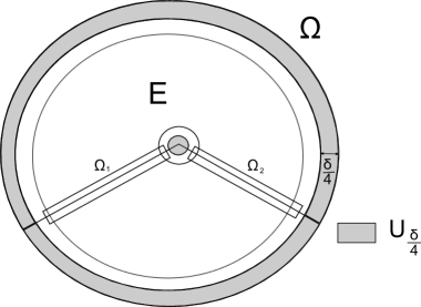
Figure 3: Construction in Step 2.

Step 2. Consider now the case in which

$$v=\chi_{E}-\chi_{\Omega\backslash E},$$

where $\mbox{Per}_{\Omega}(E)<\infty$ and $E$ has the form $E=P\cap\Omega$ with $P$ a polyhedron, i.e., there is $L\in\mathbb{N}$ such that $\partial P=H_{1}\cup H_{2}\cup\dots\cup H_{L}\cup F$ with pairwise disjoint relatively open convex polyhedra $H_{i}$ of dimension $d-1$, $H_{i}\subset\{x\in\mathbb{R}^{d}:\,(x-x_{i})\cdot\nu_{i}=0\}$ for some $x_{i}\in\mathbb{R}^{d}$ and $\nu_{i}\in S^{d-1}$, $i=1,\dots,L$, and $F$ is the union of a finite number of convex polyhedra of dimension $d-2$. Finally, we assume that $E$ meets the boundary of $\Omega$ transversally, more precisely

$$\partial\Omega\cap\partial P\mbox{ is the union of a finite number of $C^{1}$ manifolds of dimension $d-2$}.$$ (6.11)

We extend $v$ to $\mathbb{R}^{d}$ by setting

$$v(x):=\chi_{P}(x)-\chi_{\mathbb{R}^{d}\setminus P}(x),$$

and define

$$\varphi_{n}:=v\ast\Psi_{\varepsilon_{n}}$$ (6.12)

with mollifiers $\Psi_{\varepsilon_{n}}$ (see (4.6)). For fixed (small) $0<\delta<1$ set

$$U_{\delta}:=\left\{x\in\Omega:\,\mbox{dist}(x,\partial\Omega\cup F)\leq\delta\right\}$$

and let $H_{i}^{\prime}$ be relatively open subsets of $H_{i}$ with a $d-2$ dimensional $C^{\infty}$ boundary such that

$$\left\{x\in H_{i}\cap\Omega:\,\mbox{dist}(x,\partial\Omega\cup F)\geq\frac{\delta}{2}\right\}\subset H_{i}^{\prime}\subset\overline{H_{i}^{\prime}}\subset H_{i}\cap\Omega$$

and $\overline{H_{i}^{\prime}}\cap U_{\frac{\delta}{4}}=\emptyset$. Fix $0<\eta<\delta/2$, and set for every $i=1,2,\dots,L$,

$$\Omega_{i}:=\left\{x+t\nu_{i}:\,x\in H_{i}^{\prime},\,|t|<\eta\right\}.$$

Taking $\eta$ sufficiently small we may assume, without loss of generality, that $\Omega_{1},\dots,\Omega_{L}$ are pairwise disjoint and

$$\overline{\Omega_{i}}\cap U_{\frac{\delta}{4}}=\emptyset.$$ (6.13)

We apply Step 1 to every $\Omega_{i}$ to obtain a sequence $\{w_{n}^{i}\}\subset W^{3,2}(\Omega_{i})$ such that $w_{n}^{i}\rightarrow v$ in $L^{2}(\Omega_{i})$, and $\lim_{n\rightarrow\infty}\mathcal{F}_{\varepsilon_{n}}[w_{n}^{i};\Omega_{i}]\leq(m_{d}+\rho)\mathcal{H}^{d-1}(H_{i}\cap\Omega_{i})$. For every $\delta>0$ choose cut-off functions $\eta_{\delta}\in C_{c}^{\infty}(\mathbb{R}^{d};[0,1])$ such that

$$\eta_{\delta}=0\mbox{\ in\ }U_{\delta},\quad\eta_{\delta}=1\mbox{\ in\ }\mathbb{R}^{d}\setminus U_{2\delta},\quad\|\nabla^{k}\eta_{\delta}\|_{L_{\infty}(\mathbb{R}^{d})}\leq C/\delta^{k}\mbox{\ for\ }k=1,2,3.$$ (6.14)

Define $V_{n}$ by

$$V_{n}:=\begin{cases}\eta_{\delta}w_{n}^{i}+(1-\eta_{\delta})\varphi_{n}&\mbox{in\ }\overline{\Omega_{i}},\quad i=1,\dots,L,\\ \eta_{\frac{\delta}{8}}\varphi_{n}&\mbox{in\ }A:=\Omega\setminus(\overline{\Omega_{1}}\cup\dots\cup\overline{\Omega_{L}}).\end{cases}$$ (6.15)

We claim that $V_{n}\in W^{3,2}(\Omega)$ and satisfies Neumann boundary conditions on $\partial\Omega$. Indeed, considering $V_{n}$ in the neighborhood of $\partial A$, we observe that by construction of $w_{n}^{i}$ in Step 1

$$w_{n}^{i}(x)=v(x)\quad\mbox{ for }x\in\overline{\Omega_{i}}\mbox{ and }\mbox{dist}(x,H_{i})\geq\frac{\varepsilon_{n}}{2\varepsilon_{0}}.$$

Hence, from (6.12), for sufficiently large $n$ we have $w_{n}^{i}=\varphi_{n}$ in a neighborhood of $\{x\in\partial\Omega_{i}:\mbox{dist}(x,H_{i})=\eta\}$ (the part of $\partial\Omega_{i}$ parallel to $H_{i}$), and by (6.13) in that region both $\eta_{\delta}w_{n}^{i}+(1-\eta_{\delta})\varphi_{n}$ and $\eta_{\frac{\delta}{8}}\varphi_{n}$ are equal to $\varphi_{n}$. In addition, $\{x\in\partial\Omega_{i}:\mbox{dist}(x,H_{i})<\eta\}$ (the part of $\partial\Omega_{i}$ orthogonal to $H_{i}$) is contained in $U_{\delta}\backslash U_{\delta/4}$ and both $\eta_{\delta}w_{n}^{i}+(1-\eta_{\delta})\varphi_{n}$ and $\eta_{\frac{\delta}{8}}\varphi_{n}$ are equal to $\varphi_{n}$ also in that region. Finally, $V_{n}$ is identically zero in a neighborhood of $U_{\frac{\delta}{8}}$ so the Neumann boundary conditions are satisfied.

Furthermore, $\lim_{n\rightarrow\infty}||V_{n}-v||_{L^{2}(\Omega)}\leq C\delta$, since $w_{n}^{i}\rightarrow v$ in $L^{2}(\Omega_{i})$ and $\varphi_{n}\rightarrow v$ in $L^{2}(\Omega\backslash U_{\frac{\delta}{8}})$. It remains to estimate the energies. By (6.12), $V_{n}$ is possibly different from $\pm 1$ only on $U_{\frac{\delta}{4}}$ and on

$$R_{n}:=\left\{x\in\Omega:\,\mbox{dist}(x,\partial P)\leq\max\{\varepsilon_{n}/(2\varepsilon_{0}),\,\varepsilon_{n}\}\right\}.$$

Using the notation from (6.15), $V_{n}=\eta_{\frac{\delta}{8}}\varphi_{n}$ on $U_{\frac{\delta}{4}}$, $V_{n}=\varphi_{n}$ on $A\backslash U_{\frac{\delta}{4}}$, $A\cap R_{n}\subset U_{\delta}$ and $\mathcal{H}^{d-1}(\partial P\cap U_{\delta})\leq C\delta$. Thus, for $n$ sufficiently large,

$$\mathcal{F}_{\varepsilon_{n}}[V_{n};A] \leq\left|{\mathcal{F}}_{\varepsilon_{n}}[\eta_{\frac{\delta}{8}}\varphi_{n};U_{\frac{\delta}{4}}]\right|+\int_{A\cap R_{n}}\Big{(}\frac{1}{\varepsilon_{n}}W(-\varepsilon_{n}^{2}\Delta\varphi_{n}+\varphi_{n})+\varepsilon_{n}|q||\nabla\varphi_{n}|^{2}+(1-2q)\varepsilon_{n}^{3}|\Delta\varphi_{n}|^{2}$$

$$+(1-q)\varepsilon_{n}^{5}|\nabla\Delta\varphi_{n}|^{2}\Big{)}dx\leq C\delta,$$

where we also used (4.7) and (6.14) to bound the derivatives of $\varphi_{n}$ and $\eta_{\frac{\delta}{8}}$, respectively. Next we estimate the energy in $\Omega_{i}$. In $\Omega_{i}\cap U_{\delta}$, $V_{n}=\varphi_{n}$ and using (4.7) yields

$${\mathcal{F}}_{\varepsilon_{n}}[V_{n};\Omega_{i}\cap U_{\delta}]={\mathcal{F}}_{\varepsilon_{n}}[V_{n};\Omega_{i}\cap U_{\delta}\cap R_{n}]\leq C\delta.$$ (6.16)

To obtain estimates inside $T:=\Omega_{i}\cap(U_{2\delta}\backslash U_{\delta})$ we first observe that

$$\partial_{x_{i}}V_{n}=w_{n}^{i}\partial_{x_{i}}\eta_{\delta}+\eta_{\delta}\partial_{x_{i}}w_{n}^{i}-\varphi_{n}\partial_{x_{i}}\eta_{\delta}+(1-\eta_{\delta})\partial_{x_{i}}\varphi_{n},$$

and arguing as in (6.10),

$$\lim_{n\rightarrow\infty}\varepsilon_{n}^{2k-1}||\nabla^{k}w_{n}^{i}||_{L^{2}(\Omega_{i}\cap U_{2\delta})}^{2}\leq C(\rho)\,\mathcal{H}^{d-1}(H_{i}\cap U_{2\delta})\leq C(\rho)\,\delta\mbox{ for }k=0,\dots 3,$$ (6.17)

where we also used the fact that $w\in W_{loc}^{3,\infty}(\mathbb{R}^{d})$. Combined with the bounds on $\varphi_{n}$ from (4.7), it follows that,

$$\int_{T}\varepsilon_{n}|\nabla V_{n}|^{2}dx =\int_{T\cap R_{n}}\varepsilon_{n}|\nabla V_{n}|^{2}dx\leq C(\rho)\Big{(}\frac{\varepsilon_{n}}{\delta^{2}}||w_{n}^{i}||_{L^{2}(T)}^{2}+\varepsilon_{n}||\nabla w_{n}^{i}||_{L^{2}(T)}^{2}+\frac{\varepsilon_{n}}{\delta^{2}}||\varphi_{n}||_{L^{2}(T)}^{2}+$$

$$+\varepsilon_{n}||\nabla\varphi_{n}||_{L^{2}(T)}^{2}\Big{)}\leq C(\rho)\left(\delta+\frac{\varepsilon_{n}}{\delta^{2}}\right).$$

Analogous calculations for the higher derivatives of $V_{n}$, yield the bound

$${\mathcal{F}}_{\varepsilon_{n}}[V_{n};\Omega_{i}\cap(U_{2\delta}\setminus U_{\delta})]\leq C(\rho)\,\delta$$ (6.18)

for $n$ sufficiently large. Next, by (6.15), (6.17) and (4.7), we have

$$\lim_{n\rightarrow\infty}\int_{\Omega_{i}\cap U_{2\delta}}\varepsilon_{n}|\nabla V_{n}|^{2}\,dx\leq C(\rho)\,\delta,$$

and hence

$$\int_{\Omega_{i}\backslash U_{2\delta}}\left\{\frac{1}{\varepsilon_{n}}W(V_{n})-\varepsilon_{n}q|\nabla V_{n}|^{2}+(1-2q)\varepsilon_{n}^{3}|\Delta V_{n}|^{2}+(1-q)\varepsilon_{n}^{5}|\nabla\Delta V_{n}|^{2}\right\}\,dx$$

$$\leq\int_{\Omega_{i}}\left\{\frac{1}{\varepsilon_{n}}W(V_{n})-\varepsilon_{n}q|\nabla V_{n}|^{2}+(1-2q)\varepsilon_{n}^{3}|\Delta V_{n}|^{2}+(1-q)\varepsilon_{n}^{5}|\nabla\Delta V_{n}|^{2}\right\}\,dx+C(\rho)\,\delta.$$

Combining (6.10), (6.16), (6.18), and (LABEL:eq:K3), we obtain for $\delta$ sufficiently small a sequence $V_{n}\in W^{3,2}(\Omega)$, with Neumann boundary conditions on $\partial\Omega$, satisfying

$$\lim_{n\rightarrow\infty}||V_{n}-v||_{L^{2}(\Omega)}\leq\rho$$

and

$$\limsup_{n\rightarrow\infty}\mathcal{F}_{\varepsilon_{n}}[V_{n}] =\limsup_{n\rightarrow\infty}\mathcal{F}_{\varepsilon_{n}}[V_{n};\Omega]\leq\limsup_{n\rightarrow\infty}\sum_{i=1}^{L}\mathcal{F}_{\varepsilon_{n}}[V_{n};\Omega_{i}]+\limsup_{n\rightarrow\infty}\mathcal{F}_{\varepsilon_{n}}[V_{n};A]$$

$$\leq(m_{d}+\rho)\sum_{i=1}^{L}\mathcal{H}^{d-1}(\Omega_{i}\cap H_{i})+C(\rho)\,\delta$$

$$\leq(m_{d}+\rho)\mathcal{H}^{d-1}(\Omega\cap\partial P)+\rho,$$

and the Limsup Inequality (2.6) follows by a standard diagonalizing argument.

Step 3. Lastly we consider the case in which the target function is

$$v=\chi_{E}-\chi_{\Omega\backslash E},$$

where $E$ is an arbitrary set of finite perimeter in $\Omega$. Since $\Omega$ is bounded and has $C^{2}$ boundary, we can approximate $E$ with smooth sets (see Remark 3.43 in [1]) and then with polyhedral sets. In particular, we may find sets $E_{k}\subset\Omega$ of the form $E_{k}=P_{k}\cap\Omega$, where $P_{k}$ are polyhedral sets satisfying (6.11) such that $\mathcal{H}^{d-1}(\partial E_{k}\cap\partial\Omega)=0$, $\chi_{E_{k}}\rightarrow\chi_{E}$ in $L^{2}(\Omega)$, and $\mbox{Per}_{\Omega}(E_{k})\rightarrow\mbox{Per}_{\Omega}(E)$ as $k\rightarrow+\infty$. We apply Step 2 to each function $v_{k}:=\chi_{E_{k}}-\chi_{\Omega\backslash E_{k}}$ to find a sequence

$$V_{n}^{k}\rightarrow v_{k}$$

satisfying

$$\limsup_{n\rightarrow\infty}{\mathcal{F}}_{\varepsilon_{n}}[V_{n}^{k};\Omega]\leq m_{d}\mathcal{H}^{d-1}(E_{k}\cap\partial P_{k})$$

and

$$\limsup_{k\rightarrow\infty}\limsup_{n\rightarrow\infty}{\mathcal{F}}_{\varepsilon_{n}}[V_{n}^{k}]\leq\limsup_{k\rightarrow\infty}\left(m_{d}\mathcal{H}^{d-1}(E_{k}\cap\partial P_{k})\right)=m_{d}\mbox{Per}_{\Omega}(E).$$

The general result now follows by a diagonalizing argument.

Appendix

We derive the energy functional (1.3) from (1.2). To eliminate the dependence on $h$ we assume that $\phi$ and $h$ satisfy the Euler-Lagrange equation

$$\frac{\delta\mathcal{E}}{\delta h}(\phi,h)=0.$$ (6.20)

After changing variables, $x:=\bar{x}/L$, $u(x):=\phi(\bar{x})$ in (1.2) we have

$$\frac{1}{L^{d}}\mathcal{E}[u,h]=\int_{\Omega}\left(f(u)+\frac{b}{2L^{2}}|\nabla u|^{2}+\frac{\sigma}{2L^{2}}|\nabla h|^{2}+\frac{\kappa}{2L^{4}}[\Delta h]^{2}+\frac{\Lambda}{L^{2}}u\Delta h\right)\,dx,$$ (6.21)

where $\Omega:=\{x/L:x\in D\}$. Assuming natural boundary conditions, the Euler-Lagrange equation (6.20) takes the form

$$\begin{cases}\Delta\left(\frac{\kappa}{L^{4}}\Delta h-\frac{\sigma}{L^{2}}h+\frac{\Lambda}{L^{2}}u\right)=0&\text{ in }\Omega,\\ \frac{\partial h}{\partial n}=0,\frac{\partial\Delta h}{\partial n}=0,\frac{\partial u}{\partial n}=0,\frac{\partial\Delta u}{\partial n}=0&\text{ on }\partial\Omega.\end{cases}$$ (6.22)

Consider the Fourier Series expansions of $h$ and $u$,

$$h=\sum_{i=0}^{\infty}h_{i}\psi_{i},\quad u=\sum_{i=0}^{\infty}u_{i}\psi_{i},$$

where $\psi_{i}$ are the eigenfunctions of $-\Delta$ on $H^{1}(\Omega)$ with Neumann boundary conditions. Denote the corresponding nonnegative eigenvalues by $\lambda_{i}^{2}$. Then, since $\psi_{0}=const$ (due to Neumann boundary conditions), we have

$$\Delta h=-\sum_{i=1}^{\infty}\lambda_{i}^{2}h_{i}\psi_{i},\mbox{\quad and\quad}\Delta^{2}h=\sum_{i=1}^{\infty}\lambda_{i}^{4}h_{i}\psi_{i},$$

and thus by (6.22)

$$\sum_{i=1}^{\infty}\lambda_{i}^{2}\left(\frac{\kappa}{L^{2}}\lambda_{i}^{2}h_{i}+\sigma h_{i}-\Lambda u_{i}\right)\psi_{i}=0.$$

Taking the $L^{2}$ inner product with $\psi_{j}$, and noting that $\left<\psi_{i},\psi_{j}\right>_{L^{2}(\Omega)}=\delta_{ij}$, we obtain

$$\lambda_{j}^{2}\left(\frac{\kappa}{L^{2}}\lambda_{j}^{2}h_{j}+\sigma h_{j}-\Lambda u_{j}\right)=0\mbox{ for }j=1,\dots,\infty.$$

Solving for $h_{j}$ yields

$$h_{j}=\frac{\Lambda u_{j}}{\sigma+(\kappa/L^{2})\lambda_{j}^{2}}\mbox{ for }j=1,\dots,\infty,$$

and

$$h(x)=\sum_{i=0}^{\infty}h_{i}\psi_{i}(x)=const+\sum_{i=1}^{\infty}h_{i}\psi_{i}(x)=const+\sum_{i=1}^{\infty}\frac{\Lambda u_{i}\psi_{i}(x)}{\sigma+(\kappa/L^{2})\lambda_{i}^{2}}.$$

Using this expansion and $\Delta\psi_{i}=-\lambda_{i}^{2}\psi_{i}$ gives

$$-\Delta h(x)=\sum_{i=1}^{\infty}\frac{\Lambda\lambda_{i}^{2}u_{i}\psi_{i}(x)}{\sigma+(\kappa/L^{2})\lambda_{i}^{2}}.$$ (6.23)

In addition, multiplying (6.22) by $h$ and integrating by parts, we obtain

$$\int_{\Omega}\left((\kappa/L^{2})(\Delta h)^{2}+\sigma|\nabla h|^{2}+\Lambda u\Delta h\right)\,dx=0,$$

and consequently

$$\frac{1}{2}\int_{\Omega}\left((\kappa/L^{2})(\Delta h)^{2}+\sigma|\nabla h|^{2}\right)\,dx=-\frac{1}{2}\int_{\Omega}\Lambda u\Delta h\,dx.$$ (6.24)

Substituting (6.24) into (6.21) yields

$$\frac{1}{L^{d}}\mathcal{E}[u,h]=\int_{\Omega}\left(f(u)+\frac{b}{2L^{2}}|\nabla u|^{2}+\frac{\Lambda}{2L^{2}}u\Delta h\right)\,dx.$$ (6.25)

To eliminate the dependence on $h$ observe that since $\langle\psi_{i},\psi_{j}\rangle_{L^{2}(\Omega)}=\delta_{ij}$, (6.23) implies that

$$\int_{\Omega}u\Delta h\,dx=-\int_{\Omega}\left(\sum_{i=0}^{\infty}u_{i}\psi_{i}(x)\right)\left(\sum_{j=1}^{\infty}\frac{\Lambda\lambda_{j}^{2}u_{j}\psi_{j}(x)}{\sigma+(\kappa/L^{2})\lambda_{j}^{2}}\right)dx=-\sum_{i=1}^{\infty}\frac{\Lambda\lambda_{i}^{2}u_{i}^{2}}{\sigma+(\kappa/L^{2})\lambda_{i}^{2}}.$$

Substituting this expression into the energy functional (6.25) yields

$$\frac{1}{L^{d}}\mathcal{E}[u] =\int_{\Omega}\left(f(u)+\frac{b}{2L^{2}}|\nabla u|^{2}\right)\,dx-\frac{1}{2L^{2}}\sum_{i=1}^{\infty}\frac{\Lambda^{2}\lambda_{i}^{2}}{\sigma+(\kappa/L^{2})\lambda_{i}^{2}}u_{i}^{2}$$

$$=\int_{\Omega}\left(f(u)+\frac{b}{2L^{2}}|\nabla u|^{2}\right)\,dx-\frac{\Lambda^{2}}{2\kappa}\sum_{i=1}^{\infty}\left(\frac{(\kappa/L^{2})\lambda_{i}^{2}+\sigma-\sigma}{\sigma+(\kappa/L^{2})\lambda_{i}^{2}}\right)u_{i}^{2}$$

$$=\int_{\Omega}\left(f(u)+\frac{b}{2L^{2}}|\nabla u|^{2}\right)\,dx-\frac{\Lambda^{2}}{2\kappa}\sum_{i=1}^{\infty}u_{i}^{2}+\frac{\Lambda^{2}}{2\kappa}\sum_{i=1}^{\infty}\left(\frac{\sigma}{\sigma+(\kappa/L^{2})\lambda_{i}^{2}}\right)u_{i}^{2}.$$ (6.26)

At this point one can use a long-wavelength approximation as suggested for example in [22] resulting in an approximation energy

$$\frac{1}{L^{d}}\mathcal{E}_{ap}[u] =\int_{\Omega}\left(f(u)+\frac{1}{2L^{2}}\left(b-\frac{\Lambda^{2}}{\sigma}\right)|\nabla u|^{2}+\frac{\Lambda^{2}\kappa}{2L^{4}\sigma^{2}}(\Delta u)^{2}\right)\,dx,$$ (6.27)

which was studied in [7, 8]. Returning to the full energy in (6.26), we have

$$\frac{1}{L^{d}}\mathcal{E}[u] =\int_{\Omega}\left(f(u)+\frac{b}{2L^{2}}|\nabla u|^{2}-\frac{\Lambda^{2}}{2\kappa}u^{2}\right)\,dx+\frac{\Lambda^{2}L^{2}\sigma}{2\kappa^{2}}\sum_{i=1}^{\infty}\frac{1}{\frac{L^{2}\sigma}{\kappa}+\lambda_{i}^{2}}u_{i}^{2}$$

$$=\int_{\Omega}\left(f(u)+\frac{b}{2L^{2}}|\nabla u|^{2}-\frac{\Lambda^{2}}{2\kappa}u^{2}+\frac{\Lambda^{2}L^{2}\sigma}{2\kappa^{2}}u\left(\frac{L^{2}\sigma}{\kappa}-\Delta\right)^{-1}u\right)\,dx$$

$$=\int_{\Omega}\left(f(u)-\frac{\Lambda^{2}}{2\kappa}u^{2}+\frac{b}{2L^{2}}|\nabla u|^{2}+\frac{\Lambda^{2}}{2\kappa}u\left({\bf{1}}-\frac{\kappa}{L^{2}\sigma}\Delta\right)^{-1}u\right)\,dx$$

$$=\frac{\Lambda^{2}}{2\kappa}\int_{\Omega}\left(\frac{2\kappa}{\Lambda^{2}}f(u)-u^{2}+\frac{\kappa b}{L^{2}\Lambda^{2}}|\nabla u|^{2}+u\left({\bf{1}}-\frac{\kappa}{L^{2}\sigma}\Delta\right)^{-1}u\right)\,dx.$$

Setting

$$\varepsilon:=\sqrt{\frac{\kappa}{L^{2}\sigma}},\quad q:=1-\frac{b\sigma}{\Lambda^{2}},\quad W(u):=\frac{2\kappa}{\Lambda^{2}}f(u),\mbox{\quad and\ }{\mathcal{F}}^{\ast}_{\varepsilon}:=\frac{1}{\varepsilon}\frac{2\kappa}{\Lambda^{2}L^{d}}\mathcal{E},$$

yields

$${\mathcal{F}}^{\ast}_{\varepsilon}[u]:=\frac{1}{\varepsilon}\int_{\Omega}\left(W(u)-u^{2}+(1-q)\varepsilon^{2}|\nabla u|^{2}+u\left({\bf 1}-\varepsilon^{2}\Delta\right)^{-1}u\right)\,dx.$$

Compliance with Ethical Standards

Part of this research was carried out at the Center for Nonlinear Analysis. The center is partially supported by NSF Grant No. DMS-0635983 and NSF PIRE Grant No. OISE-0967140. The research of I. Fonseca was partially funded by the National Science Foundation under Grant No. DMS-0905778, DMS-1411646 and that of G. Leoni under Grant No. DMS-1007989, DMS-1412095. B. Zwicknagl acknowledges support by the Deutsche Forschungsgemeinschaft through the Sonderforschungsbereich 1060 The mathematics of emergent effects.

References

[1]
L. Ambrosio, N. Fusco, and D. Pallara.
Functions of bounded variation and free discontinuity problems.
Clarendon Press, Oxford, 2000.
[2]
M. Baía, A. C. Barroso, M. Chermisi, and J. Matias.
Coupled second order singular perturbations for phase transitions.
Nonlinearity, 26(5):1271–1311, 2013.
[3]
D. Bonheure, L. Sanchez, M. Tarallo, and S. Terracini.
Heteroclinic connections between nonconsecutive equilibria of a
fourth order differential equation.
Calc. Var. Partial Differential Equations, 17(4):341–356,
2003.
[4]
A. Braides.
-convergence for beginners.
Oxford University Press, Oxford, 2002.
[5]
D. A. Brown and E. London.
Functions of lipid rafts in biological membranes.
Annual review of cell and developmental biology,
14(1):111–136, 1998.
[6]
P. B. Canham.
The minimum energy of bending as a possible explanation of the
biconcave shape of the human red blood cell.
J. Theor. Biol., 26(1):61–81, 1 1970.
[7]
M. Chermisi, G. Dal Maso, I. Fonseca, and G. Leoni.
Singular perturbation models in phase transitions for second order
materials.
Indiana Univ. Math. J., 60(2):367–410, 2011.
[8]
M. Cicalese, E. Spadaro, and C. Zeppieri.
Asymptotic analysis of a second-order singular perturbation model for
phase transitions.
Calc. Var. Partial Differential Equations, 41(1-2):127–150,
2011.
[9]
B.D. Coleman, M. Marcus, and V.J. Mizel.
On the thermodynamics of periodic phases.
Arch. Rational Mech. Anal., 117(4):321–347, 1992.
[10]
G. Dal Maso.
An Introduction to -convergence.
Progress in Nonlinear Differential Equations and their Applications.
Birkhäuser Boston, Inc., Boston, MA, 1993.
[11]
E. L. Elson, E. Fried, J. E. Dolbow, and G. M. Genin.
Phase separation in biological membranes: integration of theory and
experiment.
Annu. Rev. Biophys., 39:207, 2010.
[12]
I. Fonseca and G. Leoni.
Modern Methods in the Calculus of Variations: Spaces.
Springer Monographs in Mathematics. Springer, New York, 2007.
[13]
I. Fonseca and L. Tartar.
The gradient theory of phase transitions for systems with two
potential wells.
Proc. Roy. Soc. Edinburgh Sect. A, 111(1-2):89–102, 1989.
[14]
E. De Giorgi.
Sulla convergenza di alcune successioni d’integrali del tipo
dell’area.
Rend. Mat., 8(6):277–294, 1975.
[15]
S. Givli, H. Giang, and K. Bhattacharya.
Stability of multicomponent biological membranes.
SIAM J. Appl. Math., 72(2):489–511, 2012.
[16]
P. Grisvard.
Elliptic problems in nonsmooth domains.
Classics in Applied Mathematics. Society for Industrial and Applied
Mathematics, 2011.
[17]
W. Helfrich.
Elastic properties of lipid bilayers: theory and possible
experiments.
Z. Naturforsch. C, 28(11):693–703, 1973.
[18]
D. Hilhorst, L. A. Peletier, and R. Schätzle.
-limit for the extended Fisher-Kolmogorov equation.
Proc. Roy. Soc. Edinburgh, 132(A):141–162, 2002.
[19]
J. Jost.
Partial Differential Equations.
Graduate Texts in Mathematics. Springer, 2007.
[20]
T. Kawakatsu, D. Andelman, K. Kawasaki, and T. Taniguchi.
Phase transitions and shapes of two-component membranes and vesicles
I: strong segregation limit.
J. Phys. II (France), 3(7):971–997, 1993.
[21]
R. V. Kohn and P. Sternberg.
Local minimizers and singular perturbations.
Proc. Roy. Soc. Edinburgh Sect. A, 111(1-2):69–84, 1989.
[22]
S. Komura, N. Shimokawa, and D. Andelman.
Tension-induced morphological transition in mixed lipid bilayers.
Langmuir, 22(16):6771–6774, 2006.
[23]
S. Leibler and D. Andelman.
Ordered and curved meso-structures in membranes and amphiphilic
films.
J. Phys. France, 48(11):2013–2018, 1987.
[24]
M. Leslie.
Do lipid rafts exist?
Science, 334(6059):1046–1047, 2011.
[25]
S. Meinhardt, R. L. C. Vink, and F. Schmid.
Monolayer curvature stabilizes nanoscale raft domains in mixed lipid
bilayers.
Proc. Natl. Acad. Sci. USA, 110(12):4476–81, 3 2013.
[26]
V.J. Mizel, L.A. Peletier, and W.C. Troy.
Periodic phases in second-order materials.
Arch. Rational. Mech. Anal., 145(4):343–382, 1998.
[27]
L. Modica.
The gradient theory of phase transitions and the minimal interface
criterion.
Arch. Rational Mech. Anal., 98(2):123–142, 1987.
[28]
L.A. Peletier and W.C. Troy.
Spatial patterns described by the extended Fisher-Kolmogorov
equation: periodic solutions.
SIAM J. Math. Anal., 28(6):1317–1353, 1997.
[29]
L. Rajendran and K. Simons.
Lipid rafts and membrane dynamics.
J. Cell. Sci., 118(6):1099–1102, 2005.
[30]
X. Ren and J. Wei.
The soliton-stripe pattern in the Seul-Andelman membrane.
Phys. D, 188(3-4):277–291, 2004.
[31]
S. Rozovsky, Y. Kaizuka, and J. T. Groves.
Formation and spatio-temporal evolution of periodic structures in
lipid bilayers.
J. Am. Chem. Soc., 127(1):36–7, 1 2005.
[32]
M. Seul and D. Andelman.
Domain shapes and patterns: the phenomenology of modulated phases.
Science, 267(5197):476–483, 1995.
[33]
K. Simons and E. Ikonen.
Functional rafts in cell membranes.
Nature, 387(6633):569–72, 6 1997.
[34]
T. Taniguchi, K. Kawasaki, D. Andelman, and T. Kawakatsu.
Phase transitions and shapes of two-component membranes and vesicles
II: weak segregation limit.
J. Phys. II (France), 4:1333–1362, 1994.