2MASS photometry and kinematical studies of open cluster NGC 188

Abstract

In this paper, we present our results for the photometric and kinematical studies of old open cluster NGC 188. We determined various astrophysical parameters like limited radius, core and tidal radii, distance, luminosity and mass functions, total mass, relaxation time etc. for the cluster using 2MASS catalog. We obtained the cluster’s distance from the Sun as 1721$\pm$41 pc and log (age)= 9.85$\pm$0.05 at Solar metallicity. The relaxation time of the cluster is smaller than the estimated cluster age which suggests that the cluster is dynamically relaxed. Our results agree with the values mentioned in the literature. We also determined the cluster’s apex coordinates as ($281^{\circ}$.88, $-44^{\circ}$.76) using AD-diagram method. Other kinematical parameters like space velocity components, cluster center and elements of Solar motion etc. have also been computed.

1 Introduction

NGC 188 is one of the oldest known open clusters of the Milky Way belonging to the old Galactic disk population (Platais et al. 2003). The cluster’s spatial location in the Galaxy ($l=122^{\circ}$.8, $b=22^{\circ}$.4) makes it relatively less obscured and poorly contaminated by field stars, hence, being easy to observe (Meibom et al. 2009; Wang et al. 2015; von Hippel & Sarajedini 1998). Thus, NGC 188 has been used extensively as a classical reference to study the evolution of Galactic disk and chemical and dynamical evolution of the Galaxy. A plot of the Galactic orbit of NGC 188 is given by Carraro & Chiosi (1994). One of the reasons behind the survival of NGC 188 to this advance age may be its almost circular, highly inclined external orbit, which avoids the inner disk regions for most of the times (Bonatto et al. 2005). The cluster is known to have approximately Solar metallicity (Friel et al. 2002; Randich et al. 2003; Worthey & Jowett 2003). The color-magnitude diagram of the cluster shows a wide giant branch (Twarog 1997; Norris & Smith 1985), blue stragglers (Leonard & Linnel 1992; Dinescu et al. 1996) and various type of binaries (von Hippel & Sarajedini 1998). Knowledge of accurate fundamental parameters of the open clusters is essential for many astrophysical calibrations (Fornal et al. 2007). The age of NGC 188 remains a crucial factor and surveys like 2MASS (Skrutskie et al. 1997) have enabled such studies in the near-IR bands.

Open clusters are group of stars moving in parallel direction in space on the celestial sphere. The directions of proper motions of the stars of open clusters will converge to a point called vertex ($A_{0},D_{0}$) of the cluster. Proper motions can be used to calculate membership probabilities and taking the most probable cluster members for studying the kinematics of the cluster will provide more precise determination of the vertex.

In light of the above discussion, we studied some of the basic parameters and kinematical properties of the cluster using the 2MASS catalogue in combination with other source of data which include information of proper motion and radial velocities of the cluster members. Conclusively, many parameters like limiting radius, core radius, age, distance, mass function slope and dynamical relaxation time etc. could be estimated. Our kinematical studies of the cluster provided the convergent point of the cluster, cluster’s velocity and the components of space motion of the cluster. We also derived the elements of Solar motion with respect to NGC 188. The kinematical parameters derived by us will help in understanding the motion of the cluster in the Galaxy.

The structure of this article is as follows: in Sect. 2, we describe the data used for the present study. Section 3 explains the photometric study and the results achieved. Section 4 deals with the kinematical analysis of NGC 188. The conclusions of this paper have been given in Sect. 5.

2 Data used and reduction procedures

Due to the unavailability of all the required data in one general catalogue for the present study, we have compiled data from different sources. We have taken photometric data from 2MASS catalogue (Cutri et al. 2003). 2MASS uniformly scanned the entire sky in three near-infrared bands $(J,H,K_{s})$ to detect and characterize point sources brighter than 1 mJy in each band, with signal-to-noise ratio (SNR) greater than 10, using a pixel size of 2^′′.0.

We combined the above photometric data with kinematical data for proper motions and radial velocities. Platais et al. (2003) presented a technique to obtain precise proper motions of stars in the region of NGC 188, using old photographic plates with assorted large aperture reflectors, in combination with recent CCD Mosaic Imager frames. They used their proper motions to determine astrometric membership probabilities down to $V$=21 in the 0.75 $deg^{2}$ area around NGC 188. For our study, we consider stars with membership probabilities higher than 50 % from the catalogue given by Platais et al. (2003), which gives us 562 member stars. Geller et al. (2008) presented the results of ongoing radial velocity (RV) survey for NGC 188 by WIYN. The data set observed by 3.5-m WIYN telescope on Kitt Peak in Arizona spans a time baseline of 11 years, a magnitude range of 12$\leq V\leq$16.5 (1.18-0.94 $M_{\odot}$) and covers an area of one degree diameter on the sky. For the kinematical studies, the values of radial velocity for NGC 188 stars have been taken from Geller et al. (2008).

3 Photometric analysis

3.1 Radial density profile (RDP)

To determine radial extent of the cluster, we extracted $J,H,K_{s}$ magnitudes, positions and radial distance of stars from the cluster centre. This data set of the cluster is taken from the Vizier webpage. The RDP were built by calculating the mean surface density in concentric rings around the cluster center, $(\alpha,\delta)_{J2000}$=(00^h47^m13^s.12, $85^{\circ}$14^′51^′′). We calculated the mean surface density $\rho(r)$ of each ring using King model (King 1966), i.e.:

$\rho(r)=f_{bg}+\frac{f_{0}}{1+(\frac{r}{r_{core}})^{2}}$

where $f_{bg}$ is the background surface density and $r_{core}$ is the core radius of the cluster where the stellar density, $\rho(r)$, becomes half of its central value, $\rho_{0}$.

In addition, we can also define the limited radius of the cluster ($r_{lim}$) which represents the radius which covers the entire cluster area and reaches enough stability with the background field density (Tadross $\&$ Bendary 2014). Mathematically, $r_{lim}$ is defined as:

$r_{lim}=r_{core}\sqrt{\frac{f_{0}}{3\sigma_{bg}}-1}$

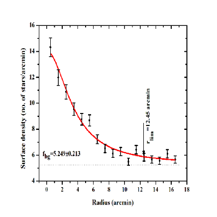
Figure 1: The radial density profile of NGC 188. Solid line denotes the fitted density distribution and the dashed line represents the background density.

Figure 1 represents the RDP of the cluster. The background stellar density is also shown with the dotted line. Solid line represent the fitted profile of the cluster. Different radii of the clusters are derived and values are listed in Table 1. Our derived values are very similar to the values given in the literature.

3.2 Color magnitude diagram (CMD) and isochrone fitting

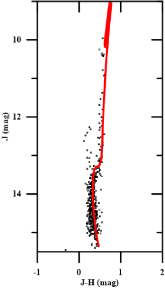
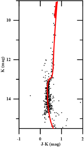
Figure 2: Theoretical Padova isochrones with Z=0.019 and log(age) = 9.85$\pm$0.05 fitted over ($J,J-H$) and ($K,J-K$) isochrones for NGC 188.

Many photometric parameters including reddening and distance modulus can be determined by fitting theoretical isochrones to the observed CMDs. Bonatto et al. (2004) fitted Padova isochrones to CMDs in ($J,J-H$) and ($K,J-K$) bands. We used the equations given by Carpenter (2001) to convert $K_{s}$ magnitudes to $K$ magnitudes. The fitting of isochrones with the observed CMDs are shown in Fig. 2. The visual best fit solar metallicity ($Z$=0.019) isochrones provide the cluster age as log(age) = 9.85.

Reddening of the cluster has been determined using Schlegel et al. (1998) and Schlafly et al. (2011). We have the coefficient ratios $A_{J}/A_{V}$ = 0.276 and $A_{H}/A_{V}$ = 0.176 , which are derived using absorption ratios by Schlegel et al. (1998), while the ratio $A_{K_{s}}/A_{V}$ = 0.118 was derived by Dutra et al. (2002). Here we have the following results for the color excess of 2MASS photometric system by Fiorucci $\&$ Munari (2003): $E_{J-H}/E_{B-V}$ = 0.309$\pm$ 0.130, $E_{J-K}/E_{B-V}$ = 0.485$\pm$ 0.150; where $R_{V}=A_{V}/E_{B-V}$ = 3.1. We used these formulae for the cluster under study to correct CMDs from the effect of reddening, i.e. $A_{K}/E_{B-V}$ = 0.365 and $A_{J}/E_{B-V}$ = 0.879. Conclusively, the distance of the cluster from the Sun can be calculated. We estimated the distance as 1721$\pm$41 pc, which we will use to study the kinematics of the cluster in Sect. 4. This distance can also be used to determine the cluster’s distance to the Galactic center ($R_{gc}$, the projected distance to the Galactic plane ($X_{\odot},Y_{\odot}$) and the distance from the Galactic plane $Z_{\odot}$ (Tadross 2012).

3.3 Luminosity and mass function

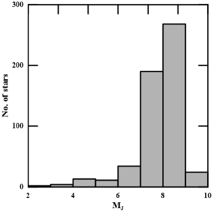
Figure 3: The apparent LF of NGC 188.

One of the main attributes of studying open clusters is to study mass function (MF) and check how it varies with different star forming conditions and stellar evolution. Mass function is derived using luminosity function (LF), which is relative number of stars in certain interval bins of absolute magnitudes. Mass function is related to the LF by a relation called mass-luminosity relation (MLR). LF for NGC188 is plotted in Fig. 3. Scalo (1986) defined the initial mass function as an empirical relation that describes the mass distribution (i.e. histogram of stellar masses) of a population of stars in terms of their theoretical initial mass (the mass they were formed with) which is mathematically defined as:

$\frac{dN}{dM}\propto M^{-{\alpha}}$

where $dN/dM$ represents the number of stars in the mass interval ($M$, $M+DM$) and $\alpha$ is a dimensionless exponent.

Salpeter (1955) established the IMF for massive stars ($>1M_{\odot}$) as $\alpha$=2.35. The steep slope of IMF indicates that during the star formation in the cluster, the number of low-mass stars is greater than high-mass stars. MLR of NGC 188 could be constructed using the adopted isochrones (Bonatto et al. 2004). The relation is a polynomial function of second order, i.e.:

$\frac{M}{M_{\odot}}=1.617385326-0.2204258896M_{K}+0.004586772674{M^{2}_{K}}$

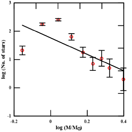
Figure 4: Mass function of open cluster NGC 188. The slope of MF is calculated as -2.90$\pm$0.21.

The MF is shown in Fig. 4 and the MF slope for NGC 188 is determined as 2.90$\pm$0.21, which is in good agreement with the Salpeter value.

3.4 Dynamical relaxation time

The relaxation time $T_{relax}$ is the time-scale on which the cluster will lose all traces of its initial condition (Yadav et al. 2013). Due to internal dynamics of the cluster, the contraction and destruction forces make the cluster approach a Maxwellian equilibrium. Through this time, low mass stars may evaporate with large random velocities trying to occupy a larger volume than the high mass stars do (Mathieu and Latham 1986). Mathematically, relaxation time has the following form (Spitzer and Hart 1971):

$$\hskip 56.9055ptT_{relax}=\frac{8.9\times 10^{5}N^{1/2}R_{h}^{3/2}}{<m>^{1/2}log(0.4N)}$$

where $R$_h is the radius containing half of the cluster mass, $N$ is the number of cluster members and $<m>$ is the average mass of the cluster stars. Using the above formula, we can calculate the dynamical relaxation time for NGC 188. Also, the dynamical evolution parameter $\tau$ can be calculated for the cluster using the formula:

$\tau=\frac{age}{T_{relax}}$.

If $\tau>>$ 1, then the cluster may be called dynamically relaxed and vice versa.

Jeffries et al. (2001) gives equation of tidal radius $r_{t}(pc)$, which depend on the total mass $M_{c}$ of the cluster, i.e.

$r_{t}=1.46\sqrt[3]{M_{c}}$.

Also, Peterson $\&$ King (1975), define the cluster concentration parameter as:

$C=log(\frac{r_{lim}}{r_{core}})$.

Table 1 presents the results of our work devoted to the photometric analysis of NGC 188 and its comparison with other published works.

4 Kinematical analysis

4.1 The vertex ($A_{0},D_{0}$) of a moving cluster

In order to compute the vetrtex using the most probable cluster members selected from Platais et al. (2003), we used apex diagram method (AD-method). This method has been used and explained in detail by Chupina et al. (2001, 2006) and Vereshchagin et al (2014). AD-diagram, plotted using individual apexes of stars represents the distribution of stars in the equatorial coordinate system. The coordinates are obtained from the solution of a geometrical problem in which the coordinates of the points of intersection of the vectors of spatial velocities of stars are displaced observation points with the celestial sphere. Figure 5 shows the AD-diagram of individual apexes of stars in the cluster region.

We followed the computation algorithm explained in Elsanhoury (2015). We present a brief preview of the process here. Let us consider a group of $N_{i}$ cluster stars at a distance $r_{i}$ (pc) with coordinates ($\alpha,\delta$), which are moving with proper motion $\mu$ (mas/yr) and radial velocity $V_{r}$ (km/sec). We used the distance value of the stars in the stellar group (cluster) under consideration as $r_{i}=1721\pm 41pc$, as calculated in Sect. 3.

The velocity components $(V_{x},V_{y},V_{z})$ along $x,y$ and $z$ axes of a coordinate system centered at the Sun can be given by the formulae given by Smart (1958):

$V_{x}=-4.74r_{i}\mu_{\alpha}\cos\delta\sin\alpha-4.74r_{i}\mu_{\delta}\sin\delta\cos\alpha+V_{r}\cos\delta\cos\alpha$

$V_{y}=+4.74r_{i}\mu_{\alpha}\cos\delta\cos\alpha-4.74r_{i}\mu_{\delta}\sin\delta\sin\alpha+V_{r}\cos\delta\sin\alpha$

$V_{z}=+4.74r_{i}\mu_{\delta}\cos\delta+V_{r}\sin\delta$

After averaging the values of $(V_{x},V_{y},V_{z})$ of different stars, we calculate the equatorial coordinates of the convergent point, as discussed in Chupina et al. (2001), i.e.:

$A_{0}=\tan^{-1}(\frac{\overline{V_{y}}}{\overline{V_{x}}})$

$D_{0}=\tan^{-1}(\frac{\overline{V_{z}}}{\sqrt{\overline{V^{2}_{x}}+\overline{V^{2}_{y}}}})$

4.2 The cluster velocity

The velocity of the cluster can be calculated by the following formula:

$V=\frac{\sum_{i=1}^{N}V_{r}^{(i)}\cos\lambda_{i}}{\sum_{i=1}^{N}\cos^{2}\lambda_{i}},$

where $\lambda$ is the angular distance from the star to apex defined as:

$\lambda_{i}=\cos^{-1}[\sin\delta_{i}\sin D_{0}+\cos\delta_{i}\cos D_{0}\cos(A_{0}-\alpha_{i})].$

4.3 The center of the cluster

The center of the cluster can be derived by the simple method of finding the equatorial coordinates of the center of mass for $N_{i}$ number of discrete objects, as following:

$x_{c}=\frac{[\sum_{i=1}^{N}r_{i}\cos\alpha_{i}\cos\delta_{i}]}{N},$

$y_{c}=\frac{[\sum_{i=1}^{N}r_{i}\sin\alpha_{i}\cos\delta_{i}]}{N},$

$z_{c}=\frac{[\sum_{i=1}^{N}r_{i}\sin\delta_{i}]}{N}.$

4.4 The components of space velocity

In order to compute components of space velocity in the Galactic space coordinates $(U,V,W)$, we use the tranformations given by Murray (1989). The formulae are given below:

$U=-0.054875539V_{x}-0.873437105V_{y}-0.483834992V_{z},$

$V=0.494109454V_{x}-0.444829594V_{y}+0.746982249V_{z},$

$W=-0.867666136V_{x}-0.198076390V_{y}+0.455983795V_{z}.$

While the mean velocities are calculates as:

$\overline{U}=\frac{\sum_{i=1}^{N}U_{i}}{N},$

$\overline{V}=\frac{\sum_{i=1}^{N}V_{i}}{N},$

$\overline{W}=\frac{\sum_{i=1}^{N}W_{i}}{N}.$

4.5 Elements of Solar motion

The Solar motion can be defined as the absolute value of the velocity of the Sun relative to the group of stars under consideration, i.e.:

$S_{\odot}=\sqrt{\overline{U}^{2}+\overline{V}^{2}+\overline{W}^{2}}(km/sec).$

The Galactic longitude ($l_{A}$) and Galactic latitude ($b_{A}$) of the Solar apex are determined as:

$l_{A}=\tan^{-1}(\frac{-\overline{V}}{\overline{U}}),$

$b_{A}=\sin^{-1}(\frac{-\overline{W}}{S_{\odot}}).$

The above three parameters $S_{\odot}$, $l_{A}$ and $b_{A}$ are called the elements of Solar motion with respect to the the group of stars under consideration.

Table 2 presents the results of the kinematical studies conducted in this article.

5 Conclusions

In the present study, we extracted photometric ($J,H,K$) data with proper motions and radial velocities from various data sources including 2MASS catalogue. The main conclusions of the present photometric and kinematic study of open cluster NGC 188 can be given as follows:

1. We have drawn the radial density profile of the cluster and determined the limiting radius and core radius according to King (1966) model. We present a CMD using most probable cluster members and determined various fundamental parameters like distance, age and reddening after correcting for interstellar reddening. The cluster’s age was derived as 7.08$\pm$0.04 Gyr using near-IR magnitude data.

2. We plotted the luminosity function and mass function diagrams for NGC 188. LF show a gradual increase towards low luminosity stars from high luminosity ones. The mass function slope, a dimensionless exponent was determined as $\alpha=$ 2.90$\pm$0.21, which is in good agreement with Salpeter’s value. The dynamical evolution parameter was found to be $\tau>>1$, which indicates that the cluster is dynamically relaxed.

3. In the kinematical studies of the cluster, we computed the apex of the cluster by AD-diagram method as $A_{0}=281^{\circ}$.88, $D_{0}=-44^{\circ}$.76. Then, we followed an algorithm to compute velocity, cluster center, space velocity and elements of solar motion for the cluster.

6 Acknowledgments

We are thankful to an anonymous referee for careful reading of the paper and constructive comments. N. V. Chupina and S. V. Vereshchagin are partly supported by the Russian Foundation for Basic Research (RFBR, grant number is 16-52-12027). Devesh P. Sariya and Ing-Guey Jiang acknowledge the grant from Ministry of Science and Technology (MOST), Taiwan. The grant numbers are MOST 103-2112-M-007-020-MY3 and NSC 100-2112-M-007-003-MY3. This publication makes use of data products from the Two Micron All Sky Survey, which is a joint project of the University of Massachusetts and the Infrared Processing and Analysis Center/California Institute of Technology, funded by the National Aeronautics and Space Administration and the National Science Foundation.

Figure 5: The AD-diagram for 562 stars with known radial velocities and having membership probability $>$50%

Table 1: The results of photometric analysis for NGC 188.

Parameters	Value	Reference	Parameters	Value	Reference
Age$(Gyr)$	7.08$\pm$0.04	Present work	$E(J-K)$	0.021	Present work
	7.0$\pm$0.5	Jiaxin et al. (2015)	$E(J-H)$	0.007	Present work
	6	Chumak et al. (2010)		0.0	Bonatto et al. (2005)
	6.2$\pm$0.2	Meibom et al. (2009)	Distance$(pc)$	1721$\pm$41	Present work
	7.0$\pm$0.5	Krusberg & Chaboyer (2006)		1714	Jiaxin et al. (2015)
	7.0$\pm$0.7	Fornal et al. (2007)		1650$\pm$50	Chumak et al. (2010)
	7.0$\pm$1.0	Bonatto et al. (2005)		1770$\pm$75	Meibom et al. (2009)
	6.8$\pm$0.7	VandenBerg & Stetson (2004)		1700$\pm$100	Fornal et al. (2007)
	6.4	Michaud et al. (2004)		1660$\pm$80	Bonatto et al. (2005)
	7.0	Sarajedini (1999)		1900	Sarajedini (1999)
	7.0	von Hippel & Sarajedini (1998)	$f_{0}(pc)$	4.38$\pm$0.19	Present work
No. of members	562	Present work	$r_{lim}(pc)$	6.23$\pm$0.65	Present work
Metallicity $(Z)$	0.019	Present work	$R_{h}(pc)$	3.12$\pm$0.33	Present work
	0.020	Jiaxin et al. (2015)		4.0	Chumak et al. (2010)
	0.015	VandenBerg & Stetson (2004)	$R_{core}(pc)$	1.91	Present work
$(m-M)_{0}$	11.188$\pm$0.06	Present work		1.89	Jiaxin et al. (2015)
	11.17$\pm$0.08	Jiaxin et al. (2015)		1.3$\pm$0.1	Bonatto et al. (2005)
	11.35	Chumak et al. (2010)		2.1	Chumak et al. (2010)
	11.24$\pm$0.09	Meibom et al. (2009)	$C$	0.55	Present work
	11.23$\pm$0.14	Fornal et al. (2007)		1.07	Jiaxin et al. (2015)
	11.1$\pm$0.1	Bonatto et al. (2005)		1.21	Chumak et al. (2010)
	11.44	von Hippel & Sarajedini (1998)		1.2$\pm$0.1	Bonatto et al. (2005)
	11.44	Sarajedini (1999)	$M_{C}(M_{\odot})$	616.5	Present work
$E(B-V)$	0.033$\pm$0.03	Present work	$<m>(M_{\odot})$	1.097	Present work
	0.036$\pm$0.01	Jiaxin et al. (2015)	$r_{t}(pc)$	12.43	Present work
	0.083	Chumak et al. (2010)		22.3	Jiaxin et al. (2015)
	0.087	Meibom et al. (2009)		21$\pm$4	Bonatto et al. (2005)
	0.025$\pm$0.005	Fornal et al. (2007)		34	Chumak et al. (2010)
	0.09	von Hippel$\&$ Sarajedini (1998)	$X_{\odot}(pc)$	$-$863.041	Present work
	0.09	Sarajedini (1999)	$Y_{\odot}(pc)$	1336.97	Present work
	0.0	Bonatto et al. (2005)	$Z_{\odot}(pc)$	655.378	Present work
	0.087	VandenBerg & Stetson (2004)	$\alpha$	2.90$\pm$0.21	Present work
$T_{relax}(Myr)$	47.09	Present work		2.15	Jiaxin et al. (2015)
	64	van den Bergh & Sher (1960)	$R_{gc}(pc)$	8672.48$\pm$74.3	Present work
$\tau$	150.35	Present work		8900$\pm$100	Bonatto et al. (2005)

Table 2: The results of kinematical analysis of NGC 188.

Parameters	Value	Reference
$(\overline{V_{x}},\overline{V_{y}},\overline{V_{z}})(km/sec)$	$(8.93,-42.46,-43.02)$	Present work
$(A_{0},D_{0})$	($281^{\circ}$.88, $-44^{\circ}$.76)	Present work
$V(km/sec)$	$-42.87\pm 0.3$	Present work
	$-42.35\pm 0.05$	Xin-Hua Gao (2014)
	$-42.36\pm 0.04$	Geller et al. (2008)
	$-42.4\pm 0.1$	Chumak et al. (2010)
$(x_{c},y_{c},z_{c})(pc)$	$(139.46,29.3,1715.08)$	Present work
$(\overline{U},\overline{V},\overline{W})(km/sec)$	$(57.41,-8.83,-18.96)$	Present work
$S_{\odot}(km/sec)$	61.1	Present work
$l_{A}$	$8^{\circ}$.745	Present work
$b_{A}$	$18^{\circ}$.08	Present work

References

- [1] Bonatto Ch., Bica E., and Girardi L., 2004, A&A, 415, 571.
- [2] Bonatto C., Bica E., and Santos Jr J. F. C., 2005, A&A, 433, 917.
- [3] Carpenter J. M., 2001, AJ, 121, 2851.
- [4] Carraro, G., and Chiosi, C. 1994, A&A, 288, 751.
- [5] Chumak, Y. O., Platais, I., McLaughlin, D. E., Rastorguev, A. S., and Chumak, O. V., 2010, MNRAS, 402, 1841.
- [6] Chupina N. V., Reva V. G., and Vereshchagin S. V., 2001, A&A, 371, 115.
- [7] Chupina N. V., Reva V. G., and Vereshchagin S. V., 2006, A&A, 451, 909.
- [8] Cutri R. M., Skrutskie M. F., van Dyk S., Beichman C. A., Carpenter J. M., Chester T., Cambresy L., Evans T., Fowler J., Gizis J., Howard E., Huchra J., Jarrett T., Kopan E. L., Kirkpatrick J. D., Light R. M., Marsh K. A., McCallon H., Schneider S., Stiening R., Sykes M., Weinberg M., Wheaton W. A., Wheelock S., and Zacarias N., 2003, VizieR On-line Data Catalog: II/246. Originally published in: 2003yCat.2246.
- [9] Dinescu D. I., Girard T. M., and van Altena W. F., Yang, T.-G., Lee, Y.-W. 1996, AJ, 111, 1205.
- [10] Dutra C. M., Santiago B. X., and Bica E., 2002, A&A, 381, 219.
- [11] Elsanhoury W. H., Astrophysics, 2015, 58, 522.
- [12] Fiorucci M., and Munari U., 2003, A&A 401, 781.
- [13] Fornal B., Tucker D. L., Smith J. A., Allam S. S., Rider C. J., and Sung H., 2007, AJ, 133, 1409.
- [14] Friel E. D., Janes K. A., Tavarez M., Scott J., Katsanis R., Lotz J., Hong L., Miller N., 2002, AJ, 124, 2693.
- [15] Geller A. M., Mathieu R. D., Harris H. C., and McClure R. D., 2008, AJ, 135, 2264.
- [16] Jeffries R. D., Thurston M. R., and Hambly N. C., 2001, A&A, 375, 863.
- [17] Jiaxin W., Jun M., Zhenyu W., Song W., and Xu Z., 2015, AJ, 150, 61.
- [18] King I. R., 1966, AJ, 71, 64.
- [19] Krusberg Z. A. C., and Chaboyer B., 2006, AJ, 131, 1565.
- [20] Leonard, P. J. T., and Linnell, A. P. 1992, AJ, 103, 1928.
- [21] Mathieu R. D., and Latham D. W., 1986, AJ, 92, 1364.
- [22] Meibom S., Grundahl, F., Clausen Jens Viggo et al. 2009, AJ, 137, 5086.
- [23] Michaud G., Richard O., and Richer J., VandenBerg D. A., 2004, ApJ, 606, 452.
- [24] Murray C. A., 1989, A&A, 218, 325.
- [25] Norris, J., and Smith, G. H. 1985, AJ, 90, 2526.
- [26] Peterson C. J., and King I. R., 1975, AJ, 80, 427.
- [27] Platais I., Kozhurina-Platais V., Mathieu R. D., Girard T. M., and van Altena W. F., 2003, AJ, 126, 2922.
- [28] Randich S., Sestito P., and Pallavicini R., 2003, A&A, 399, 133.
- [29] Salpeter E. E., 1955, ApJ, 121, 161.
- [30] Sarajedini A., von Hippel T., Kozhurina-Platais V., and Demarque P., 1999, AJ, 118, 2894.
- [31] Scalo J., 1986, Fundam. Cosm. Phys., 11, 1.
- [32] Schlafly E. F., and Finkbeiner D. P., 2011, ApJ, 737, 103.
- [33] Schlegel D. J., and Finkbeiner D. P., Davis M., 1998, ApJ, 500, 525.
- [34] Skrutskie, M., Schneider, S. E., Stiening, R., et al. 1997, in The Impact of Large Scale Near-IR Sky Surveys, ed. Garzon et al. (Netherlands: Kluwer), 210, 187.
- [35] Smart W. M., Combination of Observations, Cambridge University press, London, 1958.
- [36] Spitzer L., and Hart, M.H., 1971, ApJ., 166, 483.
- [37] Tadross A.L., 2012, RAA, 12, 158.
- [38] Tadross A. L., and Bendary, R. 2014, Journal of the Korean Astronomical Society, 47, 137.
- [39] Twarog B. A., Ashman K. M., and Anthony-Twarog B. J. 1997, AJ, 114, 2556.
- [40] van den Bergh S., Sher D., 1960, PDDO, 2, 203.
- [41] VandenBerg D. A., Stetson P. B., 2004, PASP, 116, 997.
- [42] Vereshchagin S. V., Chupina N. V., Sariya D. P., Yadav R. K. S., and Kumar B., 2014, New Astron., 31, 43.
- [43] von Hippel T., and Sarajedini A., 1998, AJ, 116, 1789.
- [44] Wang J., Ma J.,Wu Z. et al., 2015, AJ, 150, 61.
- [45] Worthey G., and Jowett k. J., 2003, PASP, 115, 96.
- [46] Xin-Hua Gao, 2014, RAA, 14, 159.
- [47] Yadav R. K. S., Sariya D. P., and Sagar, R. 2013, MNRAS, 430, 3350.
- [48]