Stochastic Runge–Kutta Software Package for Stochastic Differential Equations

Abstract

As a result of the application of a technique of multistep processes stochastic models construction the range of models, implemented as a self-consistent differential equations, was obtained. These are partial differential equations (master equation, the Fokker–Planck equation) and stochastic differential equations (Langevin equation). However, analytical methods do not always allow to research these equations adequately. It is proposed to use the combined analytical and numerical approach studying these equations. For this purpose the numerical part is realized within the framework of symbolic computation. It is recommended to apply stochastic Runge–Kutta methods for numerical study of stochastic differential equations in the form of the Langevin. Under this approach, a program complex on the basis of analytical calculations metasystem Sage is developed. For model verification logarithmic walks and Black–Scholes two-dimensional model are used. To illustrate the stochastic ‘‘predator–prey’’ type model is used. The utility of the combined numerical-analytical approach is demonstrated.

I Introduction

The mathematical models adequacy may be largely increased by taking into account stochastic properties of dynamic systems. Stochastic models are widely used in chemical kinetics, hydrodynamics, population dynamics, epidemiology, filtering of signals, economics and financial mathematics as well as different fields of physics Kloeden_Platen . Stochastic differential equations (SDE) are the main mathematical apparatus of such models.

Even for the case of ordinary differential equations (ODE) an analytical solution can be obtained only for a limited class of equations. That’s why a great variety of numerical methods have been developed Butcher_2003 ; Hairer:1::en for applications. In the case of SDE the importance of numerical methods greatly increases, because the exact analytical solutions have been obtained only for a very small number of stochastic models Kloeden_Platen ; Andreas_2003 .

Compared with numerical methods for ODEs, numerical methods for SDEs are much less developed. There are two main reasons for this: a comparative novelty of this field of applied mathematics and much more complicated mathematical apparatus. The development of new numerical methods for stochastic case in many ways is similar to deterministic methods development Burrage_1996 ; Burrage_1997 ; Burrage_1998 ; Burrage_2000 ; Rossler_2010 ; Andreas_2003 . The scheme, that has been proposed by Butcher Butcher_2003 , gives visual representation of three main classes of numerical schemes.

The accuracy of numerical scheme may be improved in the following way: by adding additional steps (multi-step), stages (multi-stage), and the derivatives of drift vector and diffusion matrix (multi-derivative) to the scheme.

Multi-step (Runge–Kutta like) numerical methods are more suitable for the program implementation, because they can be expressed as a sequence of explicit formulas. Thus, it is natural to spread Runge–Kutta methods in the case of stochastic differential equations.

The main goal of this paper is to give a review of stochastic Runge–Kutta methods implementation made by authors for Sage computer algebra system sage . The Python programming language and NumPy and SciPy modules were used for this purpose because Python programming language is an open and powerful framework for scientific calculations.

A few additional algorithms have to be implemented before proceeding to realisation of stochastic Runge-Kutta algorithm. These algorithms are: generation of Wiener process trajectories, approximation of multiple stochastic integrals, n-point distributed random values generation.

The authors have faced the necessity of stochastic numerical methods implementation in the course of work on the method of stochastization of one-step processes kulyabov:2013:conf:mmcp ; kulyabov:2014:icumt-2014:p2p ; ef-kor-gev-kul-sev:vestnik-miph:2014-3 . As The ‘‘predator-prey’’-type model was taken as an example of the methodology application in order to verify the obtained SDE models by numerical experiments. The same problem had aroused when authors developed stochastic models for RED-like queuing disciplines kulyabov:2014:icumt-2014:gns3 .

I.1 Article’s content

In the first part of the article a brief introduction of SDE’s mathematical apparatus is given. The definition of the scalar and multidimensional Wiener process, the definition of the scalar and multidimensional Itō SDEs, strong and weak convergence of the approximating function, matrix formula for double Itō integrals approximation are introduced.

The second part of the article is devoted to the description of stochastic numerical Runge–Kutta schemes with strong and weak orders of convergence for scalar and multi-dimensional Wiener processes.

The third part provides necessary information about library functions for implementation of numerical schemes from the second part of the paper.

In the final section the introduced in previous parts of the article methods are used to derive strong and weak approximations of ‘‘predator-prey’’ stochastic model. Also some conclusions about dissimilarity the stochastic version of ‘‘predator-pray’’ models from deterministic version are made based on numerical results.

The article can be regarded as a practical introduction to the field of stochastic numerical methods. Also it could be useful as guide for the implementation of stochastic numerical schemes in any other programming languages.

I.2 The choice of programming language for implementing stochastic numerical methods

The following requirements to computer algebra system’s programming language were taken into account:

• advanced tools for manipulations with multidimensional arrays (up to four axes) with a large number of element are needed;

• it is critical to be able to implement parallel execution of certain functions and sections of code due to the need of a large number of independent calculations according to Monte-Carlo method;

• functions to generate large arrays of random numbers are needed;

• software should be open and free for non-commercial use.

Computer algebra system Sage generally meets all these requirements. NumPy module is used for array manipulations and SciPy module — for n-point distribution creation.

II Wiener stochastic process

In this section only the most important definitions and notations are introduced. For brief introduction to SDE see Higham_2001 ; Malham_2010 , for more details see Kloeden_Platen ; Platen_Liberati_2010 ; Oksendal::en .

A standard scalar Wiener process $W(t)$, $t\geqslant 0$ is a stochastic process which depends continuously on $t\in[t_{0},T]$ and satisfies the following three conditions:

• $\mathrm{P}\{W(0)=0\}=1$, in other words $W(0)=0$ almost surely;

• $W(t)$ has independent increments i.e. $\{\Delta W_{i}\}^{N-1}_{0}$ — independently distributed random variables; $\Delta W_{i}=W(t_{i+1})-W(t_{i})$ and $0\leqslant t_{0}<t_{1}<t_{2}<\ldots<t_{N}\leqslant T$;

• $\Delta W_{i}=W(t_{i+1})-W(t_{i})\sim\mathcal{N}(0,t_{i+1}-t_{i})$, where $0\leqslant t_{i+1}<t_{i}<T$, $i=0,1,\ldots,N-1$.

Notation $\Delta W_{i}\sim\mathcal{N}(0,\Delta t_{i})$ denotes that $\Delta W_{i}$ is a normally distributed random variable with zero mean $\mathbb{E}[\Delta W_{i}]=\mu=0$ and unit variance $\mathbb{D}[\Delta W_{i}]=\sigma^{2}=\Delta t_{i}$.

Multidimensional Wiener process $W^{\alpha}(t)\colon\Omega\times[t_{0},T]\to\mathbb{R}^{m},\;\forall\alpha=1,\ldots,m$, is consist of independent $W^{1}(t),\ldots,W^{m}(t)$ scalar Wiener processes. The increments $\Delta W^{\alpha}_{i}$ are mutually independent normally distributed random variables with zero mean and unit variance.

II.1 Computer simulation of sample Wiener process paths

In order to construct Wiener process sample path on $[0,T]$ interval divided into $N$ parts with subinterval step $\Delta t_{i}=h=\mathrm{const}$, we need to generate $N$ normally distributed random numbers $\varepsilon_{0},\ldots,\varepsilon_{N-1}\sim\mathcal{N}(0,h)$ and find their cumulative sums $\varepsilon_{0}$, $\varepsilon_{0}+\varepsilon_{1}$, $\varepsilon_{0}+\varepsilon_{1}+\varepsilon_{2}$ and so on. As the result two arrays (each with $N$ elements) will be get. The first array W consist of Wiener sample path points and the second dW is an array of increments. For example of such trajectory see fig. 1.

In case of $m$-dimension process $m$ sequences of $N$ normally distributed random variables should be generated.

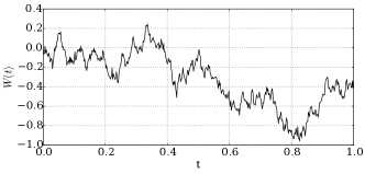
Figure 1: Wiener process path

В описываемой нами библиотеке для генерирования выборочных винеровских траекторий написана функция:

⬇

(dt, t, dW, W) = wiener_process(N, dim=1, interval=(0.0, 1.0))

Обязательны аргумент $N$ — число точек разбиения временного интервала interval (по умолчанию $[0,1]$), а dim — размерность винеровского процесса. Функция возвращает кортеж из четырех элементов, где dt — шаг разбиения ($\Delta t_{i}=h=\mathrm{const}$), t — одномерный numpy массив содержащий значения моментов времени $t_{1},t_{2},\ldots,t_{N}$, dW, W — также numpy массивы размерностью $N\times m$ содержащие приращения $\Delta W^{\alpha}_{i}$ и точки выборочной траектории $W^{\alpha}_{i}$, где $i=1,\ldots,N;\;\alpha=1,\ldots,m$.

II.2 Itô SDE for multidimensional Wiener process

Let’s consider a random process $\mathbf{x}(t)=(x^{1}(t),\ldots,x^{d}(t))^{T}$, where $\mathbf{x}(t)$ belongs to the function space $\mathrm{L}^{2}(\Omega)$ with norm $\|\cdot\|$. We assume that stochastic process $\mathbf{x}(t)$ is a solution of Itō SDE Oksendal::en ; Kloeden_Platen :

$$x^{\alpha}(t)=f^{\alpha}(t,x^{\gamma}(t))\mathrm{d}t+\sum\limits_{\beta=1}^{m}G^{\alpha}_{\beta}(t,x^{\gamma}(t))\mathrm{d}W^{\beta},$$

where $\alpha,\gamma=1,\ldots,d$, $\beta=1,\ldots,m$, vector value function $f^{\alpha}(t,x^{\gamma}(t))=$ $f^{\alpha}(t,x^{1}(t),\ldots,x^{d}(t))$ is a drift vector, and matrix value function $g^{\alpha}_{\beta}(t,x^{\gamma}(t))$ is a diffusion matrix, $W^{\alpha}=(W^{1},\dots,W^{m})^{T}$ is a multidimensional Wiener process, also known as a driver process of SDE.

Let’s introduce the discretization of interval $[t_{0},T]$ by sequence $t_{0}<t_{1}<\ldots<t_{N}=T$ with step $h_{n}=t_{n+1}-t_{n}$, where $n=0,\ldots,N-1$ and $h=\max{\{h_{n-1}\}^{N}_{1}}$ — minimal step. We also consider the step $h_{n}=h$ to be a constant; $\mathbf{x}_{n}$ — mesh function for random process $\mathbf{x}(t)$ approximation, i.e. $\mathbf{x}_{0}=\mathbf{x}(t_{0})$, $\mathbf{x}_{n}\approx\mathbf{x}(t_{n})\;\forall n=1,\ldots,N$.

II.3 Strong and weak convergences of approximation function

It is necessary to define the criterion for measuring the accuracy of process $\mathbf{x}(t)$ approximation by sequences of functions $\{\mathbf{x}_{n}\}^{N}_{1}$. Usually strong and weak Oksendal::en ; Andreas_2003 ; Rossler_2010 criteria are defined.

The sequence of approximating functions $\{\mathbf{x}_{n}\}^{N}_{1}$ converges with order $p$ to exact solution $\mathbf{x}(t)$ of SDE in moment $T$ in strong sense if constant $C>0$ exists and $\delta_{0}>0$, such as $\forall h\in(0,\delta_{0}]$ the condition

$$\mathbb{E}(\|\mathbf{x}(T)-\mathbf{x}_{N}\|)\leqslant Ch^{p}$$

is fulfilled.

The sequence of approximating functions $\{\mathbf{x}_{n}\}^{N}_{1}$ converges with order $p$ to solution $\mathbf{x}(t)$ of SDE in moment $T$ in weak seance if constant $C_{F}>0$ exists and $\delta_{0}>0$, such as $\forall h\in(0,\delta_{0}]$ the condition

$$\left|\mathbb{E}\left[F(\mathbf{x}(T))\right]-\mathbb{E}\left[F(\mathbf{x}_{N})\right]\right|\leqslant C_{F}h^{p}$$

is fulfilled.

$F\in C^{2(p+1)}_{\mathrm{P}}(\mathbb{R},\mathbb{R}^{d})$ is continuously differentiable (including $2(p+1)$-th derivatives) functional with polynomial growth.

If the matrix $\mathbf{G}$ vanishes, the condition of strong convergence is equivalent to the deterministic case convergence condition. In contrast to the deterministic case the order of strong convergence is not necessarily a natural number and may take the rational fractional values.

The convergence type selection depends entirely on the problem being solved. Numerical methods with a strong convergence are the best choice for specific trajectory approximation of a random process $\mathrm{x}(t)$ and therefore the information on the driving Wiener process ia necessary. In practice, this means that the function, that implements the method with strong stochastic convergence, must get two-dimensional array with increments of $\Delta W^{\alpha}_{n}$, where $\alpha=1,\ldots,m;\;n=1,\ldots,N$. This array will be also used for the approximation of multiple stochastic integrals.

Weak numerical methods are suitable for approximation of characteristics of the random process $\mathrm{x}(t)$ probability distribution, because no information about the trajectory driving Wiener process is required, and random values for these methods can be generated on some other probability space, which is easy to implement in software.

II.4 Approximation of Itô multiple stochastic integrals

In general, for the design of numerical schemes with the order of the strong convergence grater than $p=\frac{1}{2}$, it is necessary to include single and double Itô integrals in the these schemes formula:

$$I^{i}(t_{n},t_{n+1})=I^{i}(h_{n})=\int\limits_{t_{n}}^{t_{n+1}}\mathrm{\mathrm{d}}W^{i}(\tau),$$ (1)

$$I^{ij}(t_{n},t_{n+1})=I^{ij}(h_{n})=\int\limits_{t_{n}}^{t_{n+1}}\int\limits_{t_{n}}^{\tau_{1}}\mathrm{d}W^{i}(\tau_{2})\mathrm{d}W^{j}(\tau_{1}),$$ (2)

where $i,j=1\ldots,m$ and $W^{i}$ are components of Wiener process.

So the main task is to express Itô integrals in terms of Wiener process increments $\Delta W^{i}_{n}=W^{i}(t_{n+1})-W^{i}(t_{n})$. In the case of single integral it is possible for any index $i$: $I^{i}(h_{n})=\Delta W^{i}_{n}$. The case of double $I^{ij}(h_{n})$ integral is more complicated and there is an exact formula only for $i=j$ case:

$$I^{ii}(h_{n})=\dfrac{1}{2}\left((\Delta W^{i}_{n})^{2}-\Delta t_{n}\right).$$

In other cases, i.e. $i\neq j$ for $I^{ij}(h_{n})$, the exact expression with increments $\Delta W^{\alpha}_{n}$ and $\Delta t_{n}$ do not exist, so the numerical approximation shell be used.

In paper Wiktorsson_2001 author introduced a matrix form of approximation formulas. Let’s denote as $\mathbf{1}_{m\times m}$ and $\mathbf{0}_{m\times m}$ the unit and zero matrices $m\times m$. Then

$$\mathbf{I}(h_{n})=\dfrac{\Delta\mathbf{W}_{n}\Delta\mathbf{W}_{n}-h_{n}\mathbf{1}_{m\times m}}{2}+\mathbf{A}(h_{n}),$$ (3)

$$\mathbf{A}(h_{n})=\dfrac{h}{2\pi}\sum\limits^{\infty}_{k=1}\dfrac{1}{k}\biggl{(}\mathbf{V}_{k}(\mathbf{U}_{k}+\sqrt{2/h_{n}}\Delta\mathbf{W}_{n})^{T}-(\mathbf{U}_{k}+\sqrt{2/h_{n}}\Delta\mathbf{W}_{n})\mathbf{V}^{T}_{k}\biggr{)},$$ (4)

where $\Delta\mathbf{W}_{n},\mathbf{V}_{k},\mathbf{U}_{k}$ are normally distributed independent multidimensional random values:

$$\Delta\mathbf{W}_{n}=(\Delta W^{1}_{n},\Delta W^{2}_{n},\ldots,\Delta W^{m}_{n})^{T}\sim\mathcal{N}(\mathbf{0}_{m\times m},h_{n}\mathbf{1}_{m\times m}),$$ (5)

$$\mathbf{V}_{k}=(V^{1}_{k},V^{2}_{k},\ldots,V^{m}_{k})^{T}\sim\mathcal{N}(\mathbf{0}_{m\times m},\mathbf{1}_{m\times m}),$$ (6)

$$\mathbf{U}_{k}=(U^{1}_{k},U^{2}_{k},\ldots,U^{m}_{k})^{T}\sim\mathcal{N}(\mathbf{0}_{m\times m},\mathbf{1}_{m\times m}).$$ (7)

II.5 SDEs with exact solutions

For verification of written programs in the case of strong convergence SDEs with a known analytical solution will be used, so it makes possible to compute the error of trajectories approximation.

II.6 Logarithmic walk (one-dimensional Wiener process)

As an example of SDE with known exact solution the logarithmic walk model Platen_Liberati_2010 ; Kloeden_Platen is used:

$$\mathrm{d}x(t)=\mu x(t)\mathrm{d}t+\sigma x(t)\mathrm{d}W(t),\;\;x(0)=x_{0},$$

the exact solution is (Kloeden_Platen, , section 4.4):

$$x(t)=x_{0}\exp{\left((\mu-0.5\sigma^{2})t+\sigma W(t)\right)}.$$

Initial values are $\mu=2,\;\sigma=1$ and $x_{0}=1$.

II.7 Two-dimensional Black–Scholes model

For two dimensional Wiener process the two-dimensional Black–Scholes model Platen_Liberati_2010 is used in following form:

$$\mathbf{x}(t)=\mathrm{A}\mathbf{x}(t)\mathrm{d}t+\sum\limits^{2}_{k=1}\mathrm{B}_{k}\mathbf{x}(t)\mathrm{d}W^{k},$$

all matrices are diagonal: $A=\mathrm{diag}(a^{1},a^{2})$, $B_{1}=\mathrm{diag}(b^{1}_{1},b^{2}_{1})$ and $B_{2}=\mathrm{diag}(b^{1}_{2},b^{2}_{2})$. Drift vector $\mathbf{f}(\mathbf{x})$ and diffusion matrix $\mathrm{G}(\mathbf{x})$ can be written as

$$\mathrm{f}(\mathbf{x})=\begin{bmatrix}a^{1}x^{1}(t)\\ a^{2}x^{2}(t)\end{bmatrix},\;\;\mathrm{G}(\mathbf{x})=\begin{bmatrix}b^{1}_{1}x^{1}(t)&b^{1}_{2}x^{1}(t)\\ b^{2}_{1}x^{2}(t)&b^{2}_{2}x^{2}(t)\end{bmatrix}.$$

The exact analytical solution is given by

$$\mathbf{x}(t)=\mathbf{x}_{0}\exp\left\{\left(\mathrm{A}-\frac{1}{2}\sum\limits^{2}_{k=1}B_{k}^{2}\right)t+\sum\limits^{2}_{k=1}\mathrm{B}_{k}W^{k}(t)\right\}.$$

For calculations we will take matrices: $A=\mathrm{diag}(a_{1},a_{2})$, $B_{1}=\mathrm{diag}(b_{1},b_{2}\rho)$, $B_{2}=\mathrm{diag}(0,b_{2}\sqrt{1-\rho})$, and following values of parameters $x^{1}_{0}=x^{1}_{0}=1.0$, $a_{1}=a_{2}=0.1$, $b_{1}=b_{2}=0.2$, $\rho=0.8$. Then the exact solution of the equation takes the form:

$$x^{1}(t)=x^{1}_{0}\exp\left((a_{1}-0.5b^{2}_{1})t+b_{1}W^{1}(t)\right)$$

$$x^{2}(t)=x^{2}_{0}\exp\left((a_{2}-0.5b^{2}_{2})t+b_{2}\left(\rho W^{1}(t)+\sqrt{1+\rho^{2}}W^{2}(t)\right)\right).$$

III Stochastic Runge-Kutta methods

In this section some of the most effective stochastic numerical Runge–Kutta methods are presented (based on the papers Rossler_2010 ; Andreas_2003 ; Debrabant_2007 ; Debrabant_2013 ; Tocino_2001 ; Soheili_2007 ; Mackevicius_1994 ). We restrict ourselves to the numerical schemes without derivatives of drift vector and diffusion matrix, so the effective Milstein schemes will be neglected Milstein_1974 ; Milstein_1979 ; Milstein_1986 .

In the beginning we will mention some factors that make stochastic Runge–Kutta methods more complicated in comparison to classical methods:

• When selecting a particular method we must take into account what type of convergence is necessary to provide for this specific stochastic model, and also which type of the stochastic equations is to be solved — Itô form or the Stratonovich form. This increases the number of algorithms to be programmed.

• For methods with a strong convergence of $p_{s}>1$ the approximation of double stochastic integrals is required and this is a very expensive computational task.

• In the numerical scheme there are not only matrices and vectors but also tensors (four-dimensional arrays). So convolution operation on several indices is required. Implementation of convolution operation as summation by means of cycles leads to a significant drop of performance.

• In order to use the weak methods, Monte Carlo method should be applied and several series of calculations ($10^{7}$-$10^{8}$ calculations in each series) are required.

The program operation speed depends greatly on the necessity of multidimensional arrays convolution. NumPy module provides very useful function einsum (Einstein summation) which greatly improves the speed of convolution calculation.

It is also important to pay attention to the large number of zeros in generalized Butcher tables. Implementation of a separate function for specific method often helps to get a performance goal in comparison with the function that implements a universal algorithm.

III.1 Euler–Maruyama numerical method

The simplest numerical method for solving both scalar equations and systems of SDEs is Euler-Maruyama method, named in honor of Gishiro Maruyama (Gisiro Maruyama), who extends the classical Euler’s method from ODE to SDE case Maruyama_1955 . The method is easily generalized to the case of multidimensional Wiener process:

$$x^{\alpha}_{0}=x^{\alpha}(t_{0}),$$

$$x^{\alpha}_{n+1}=x^{\alpha}_{n}+f^{\alpha}(t_{n},x^{\alpha}_{n})h_{n}+\sum\limits^{d}_{\gamma=1}G^{\alpha}_{\beta}(t_{n},x^{\gamma}_{n})\Delta W^{\beta}_{n}.$$

As seen from the formulas, on each step only the increment of the driving Wiener process $\Delta W^{\beta}_{n}$ is required. The method has a strong $(p_{d},p_{s})=(1.0,0.5)$ order. The $p_{d}$ value denotes the accuracy order of the deterministic numerical method, i.e. the precision that a numerical method will give being applied to the equation with $G(t,x^{\alpha}(t))\equiv 0$. The $p_{s}$ value denotes the order of approximation of the stochastic part of the equation.

III.2 Strong stochastic Runge–Kutta methods for SDEs with scalar Wiener process

In the case of scalar SDE and Wiener process the following scheme is valid:

$$X^{i}_{0}=x_{n}+\sum\limits^{s}_{j=1}A_{0j}^{i}f(t_{n}+c^{j}_{0}h_{n},X^{j}_{0})h_{n}+\sum\limits^{s}_{j=1}B^{i}_{0j}g(t_{n}+c^{j}_{1}h_{n},X^{j}_{1})\dfrac{I^{10}(h_{n})}{\sqrt{h_{n}}},$$ (8)

$$X^{i}_{1}=x_{n}+\sum\limits^{s}_{j=1}A_{1j}^{i}f(t_{n}+c^{j}_{0}h_{n},X^{j}_{0})h_{n}+\sum\limits^{s}_{j=1}B^{i}_{1j}g(t_{n}+c^{j}_{1}h_{n},X^{j}_{1})\sqrt{h_{n}},$$ (9)

$$x_{n+1}=x_{n}+\sum\limits^{s}_{i=1}a_{i}f(t_{n}+c^{i}h_{n},X^{i}_{0})h_{n}+$$ (10)

$$\qquad+\sum\limits^{s}_{i=1}\left(b^{1}_{i}I^{1}(h_{n})+b^{2}_{i}\dfrac{I^{11}(h_{n})}{\sqrt{h_{n}}}+b^{3}_{i}\dfrac{I^{10}(h_{n})}{h_{n}}+b^{4}_{i}\dfrac{I^{111}(h_{n})}{h_{n}}\right)g(t_{n}+c^{i}_{1},X^{i}_{1}).$$ (11)

The method is characterized by the Butcher table Rossler_2010 :

$${\begin{array}[]{c|c|c|c}c^{i}_{0}&A^{i}_{0j}&B^{i}_{0j}&\\ \hline\cr c^{i}_{1}&A^{i}_{1j}&B^{i}_{1j}&\\ \hline\cr&a_{i}&b^{1}_{i}&b^{2}_{i}\\ \hline\cr&&b^{3}_{i}&b^{4}_{i}\\ \end{array}}.$$

In Rößler preprint Rossler_2010 there are two realisations of this scheme for $s=4$:

$${\begin{array}[]{c|cccc|cccc|cccc}0&0&0&0&0&0&0&0&0&&&\\ \frac{3}{4}&\frac{3}{4}&0&0&0&\frac{3}{2}&0&0&0&&&\\ 0&0&0&0&0&0&0&0&0&&&\\ 0&0&0&0&0&0&0&0&0&&&\\ \hline\cr 0&0&0&0&0&0&0&0&0&&&\\ \frac{1}{4}&\frac{1}{4}&0&0&0&\frac{1}{2}&0&0&0&&&\\ 1&1&0&0&0&-1&0&0&0&&&\\ \frac{1}{4}&0&0&\frac{1}{4}&0&-5&3&\frac{1}{2}&0&&&\\ \hline\cr&\frac{1}{3}&\frac{2}{3}&0&0&-1&\frac{4}{3}&\frac{2}{3}&0&-1&\frac{4}{3}&-\frac{1}{3}&0\\ \hline\cr&&&&&2&-\frac{4}{3}&-\frac{2}{3}&0&-2&\frac{5}{3}&-\frac{2}{3}&1\end{array}}\;\;{\begin{array}[]{c|cccc|cccc|cccc}0&0&0&0&0&0&0&0&0&&&\\ 1&\frac{3}{4}&0&0&0&0&0&0&0&&&\\ \frac{1}{2}&\frac{1}{4}&\frac{1}{4}&0&0&1&\frac{1}{2}&0&0&&&\\ 0&0&0&0&0&0&0&0&0&&&\\ \hline\cr 0&0&0&0&0&0&0&0&0&&&\\ \frac{1}{4}&\frac{1}{4}&0&0&0&-\frac{1}{2}&0&0&0&&&\\ 1&1&0&0&0&1&0&0&0&&&\\ \frac{1}{4}&0&0&\frac{1}{4}&0&2&-1&\frac{1}{2}&0&&&\\ \hline\cr&\frac{1}{6}&\frac{1}{6}&\frac{2}{3}&0&-1&\frac{4}{3}&\frac{2}{3}&0&1&-\frac{4}{3}&\frac{1}{3}&0\\ \hline\cr&&&&&2&-\frac{4}{3}&-\frac{2}{3}&0&-2&\frac{5}{3}&-\frac{2}{3}&1\end{array}}.$$

The first scheme we will denote as SRK1W1, the second — as SRK2W2. The method SRK1W1 has strong order $(p_{d},p_{s})=(2.0,1.5)$, the method SRK2W1 has strong order $(p_{d},p_{s})=(3.0,1.5)$. Another scheme with strong order $p_{s}=1.0$ can be found in Kloeden_Platen . This is the method with following Butcher table:

$$\text{{KlPl}: }{\begin{array}[]{c|cc|cc|cc}0&0&0&0&0&&\\ 0&0&0&0&0&&\\ \hline\cr 0&0&0&0&0&&\\ 0&0&0&0&0&&\\ \hline\cr 0&1&0&1&0&-1&1\\ &&&1&0&0&0\\ \end{array}}$$

On the figure. 2 the local error of approximation of SDE exact solution for logarithmic walk model is presented. The realisation of strong stochastic Runge–Kutta method with order $p_{s}=1.5$ of strong convergence was used. It is interesting to note, that the approximation of deterministic parts of the methods SRK1W1 and SRK2W1 don’t essentially affect the error value.

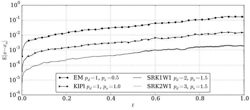
Figure 2: The errors of methods for scalar process $W$ with $h=10^{-3}$

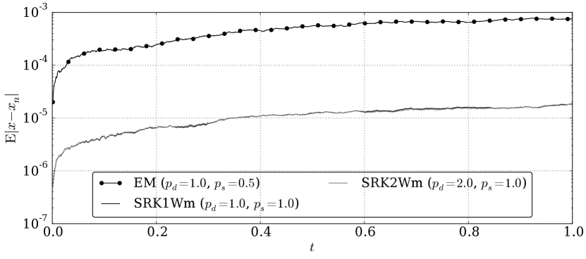
Figure 3: The errors of methods for double process $W^{\alpha}$ with $h=10^{-3}$

III.3 Strong stochastic Runge–Kutta methods for SDE system with multidimensional Wiener process

For Itô SDE system with multidimensional Wiener process the stochastic Runge-Kutta scheme with strong order $p_{s}=1.0$ can be obtained using single and double Itô integrals Rossler_2010 .

$$X^{0i\alpha}=x^{\alpha}_{n}+\sum\limits^{s}_{j=1}A^{i}_{0j}f^{\alpha}(t_{n}+c^{j}_{0}h_{n},X^{0j\beta})h_{n}+\sum\limits_{l=1}^{m}\sum\limits^{s}_{j=1}B^{i}_{0j}G^{\alpha}_{l}(t_{n}+c^{j}_{1}h_{n},X^{lj\beta})I^{l}(h_{n}),$$

$$X^{ki\alpha}=x^{\alpha}_{n}+\sum\limits^{s}_{j=1}A^{i}_{1j}f^{\alpha}(t_{n}+c^{j}_{0}h_{n},X^{0j\beta})h_{n}+\sum\limits_{l=1}^{m}\sum\limits^{s}_{j=1}B^{i}_{1j}G^{\alpha}_{l}(t_{n}+c^{j}_{1}h_{n},X^{lj\beta})\dfrac{I^{lk}(h_{n})}{\sqrt{h_{n}}},$$

$$x^{\alpha}_{n+1}=x^{\alpha}_{n}+\sum\limits^{s}_{i=1}a_{i}f^{\alpha}(t_{n}+c^{i}_{0}h_{n},X^{0i\beta})h_{n}+\sum\limits^{m}_{k=1}\sum\limits^{s}_{i=1}(b^{1}_{i}I^{k}(h_{n})+b^{2}_{i}\sqrt{h_{n}})G^{\alpha}_{k}(t_{n}+c^{i}_{1}h_{n},X^{ki\beta}),$$

where $n=0,1,\ldots,N-1$; $i=1,\ldots,s$; $\beta,k=1,\ldots,m$; $\alpha=1,\ldots,d$.

Butcher table Rossler_2010 has the form:

$${\begin{array}[]{c|c|c|c}c^{i}_{0}&A^{i}_{0j}&B^{i}_{0j}&\\ \hline\cr c^{i}_{1}&A^{i}_{1j}&B^{i}_{1j}&\\ \hline\cr&a_{i}&b^{1}_{i}&b^{2}_{i}\\ \end{array}}.$$

There are two realisations of this scheme for $s=3$ in Rößler preprint Rossler_2010 :

$$\text{{SRK1Wm}: }{\begin{array}[]{c|ccc|ccc|ccc}0&0&0&0&0&0&0&&&\\ 0&0&0&0&0&0&0&&&\\ 0&0&0&0&0&0&0&&&\\ \hline\cr 0&0&0&0&0&0&0&&&\\ 0&0&0&0&1&0&0&&&\\ 0&0&0&0&-1&0&0&&&\\ \hline\cr&1&0&0&1&0&0&0&\frac{1}{2}&\frac{1}{2}\end{array}}\;\;\text{{SRK2Wm}: }{\begin{array}[]{c|ccc|ccc|ccc}0&0&0&0&0&0&0&&&\\ 1&1&0&0&0&0&0&&&\\ 0&0&0&0&0&0&0&&&\\ \hline\cr 0&0&0&0&0&0&0&&&\\ 1&1&0&0&1&0&0&&&\\ 1&1&0&0&-1&0&0&&&\\ \hline\cr&\frac{1}{2}&\frac{1}{2}&0&1&0&0&0&\frac{1}{2}&-\frac{1}{2}\end{array}}$$

The SRK1Wm method has the strong order $(p_{d},p_{s})=(1.0,1.0)$ of convergence and the method SRK2Wm has the strong order $(p_{d},p_{s})=(2.0,1.0)$ of convergence.

On figure 3 the graph of strong convergence local error for Black–Scholes model is presented. It is also important to mention, that the deterministic part of methods SRKp1W1 and SRKp2W1 does not essentially influence the error value.

III.4 Stochastic Runge–Kutta methodes with weak convergence of $p=2.0$ order

Numerical methods with weak convergence are the best for approximation of characteristics of the distribution of the random process $x^{\alpha}(t)$. Weak numerical method does not require information about the exact trajectory of a Wiener process $W^{\alpha}_{n}$, and the random variables for these methods can be generated on another probability space. So we can use distribution which is easily generated on the computer.

For Itô SDE system with multidimensional Wiener process the following stochastic Runge-Kutta scheme with weak order $p_{s}=2.0$ is valid Rossler_2010 .

$$X^{0i\alpha}=x^{\alpha}_{n}+\sum\limits^{s}_{j=1}A_{0j}^{i}f^{\alpha}(t_{n}+c^{j}_{0}h_{n},X^{0j\beta})h_{n}+\sum\limits^{s}_{j=1}\sum\limits^{m}_{l=1}B_{0j}^{i}G^{\alpha}_{l}(t_{n}+c^{j}_{1}h_{n},X^{lj\beta})\hat{I}^{l},$$

$$X^{ki\alpha}=x^{\alpha}_{n}+\sum\limits^{s}_{j=1}A^{i}_{1j}f^{\alpha}(t_{n}+c^{j}_{0}h_{n},X^{0j\beta})h_{n}+\sum\limits^{s}_{j=1}B^{i}_{1j}G^{\alpha}_{k}(t_{n}+c_{1}^{j}h_{n},X^{kj\beta})\sqrt{h_{n}},$$

$$\widehat{X}^{ki\alpha}=x^{\alpha}_{n}+\sum\limits^{s}_{j=1}A^{i}_{2j}f^{\alpha}(t_{n}+c^{j}_{0}h_{n},X^{0j\beta})h_{n}+\sum\limits^{s}_{j=1}\sum\limits^{m}_{l=1,l\neq k}B^{i}_{2j}G^{\alpha}_{l}(t_{n}+c_{1}^{j}h_{n},X^{lj\beta})\frac{\hat{I}^{kl}}{\sqrt{h_{n}}},$$

$$x^{\alpha}_{n+1}=x^{\alpha}_{n}+\sum\limits^{s}_{i=1}a_{i}f^{\alpha}(t_{n}+c^{i}_{1},X^{ki\beta})h_{n}+\sum\limits^{s}_{i=1}\sum\limits^{m}_{k=1}\left(b^{1}_{i}\hat{I}^{k}+b^{2}_{i}\frac{\hat{I}^{kk}}{\sqrt{h_{n}}}\right)G^{\alpha}_{k}(t_{n}+c^{i}_{1}h_{n},X^{ki\beta})+$$

$$+\sum\limits^{s}_{i=1}\sum\limits^{m}_{k=1}\left(b^{3}_{i}\hat{I}^{k}+b^{4}_{i}\sqrt{h_{n}}\right)G^{\alpha}_{k}(t_{n}+c^{i}_{2}h_{n},\widehat{X}^{ki\beta}).$$

Butcher table Rossler_2010 in this case appears as follows:

$${\begin{array}[]{c|c|c|c}c^{i}_{0}&A^{i}_{0j}&B^{i}_{0j}&\\ \hline\cr c^{i}_{1}&A^{i}_{1j}&B^{i}_{1j}&\\ \hline\cr c^{i}_{2}&A^{i}_{2j}&B^{i}_{2j}&\\ \hline\cr&a_{i}&b^{1}_{i}&b^{2}_{i}\\ \hline\cr&&b^{3}_{i}&b^{4}_{i}\\ \end{array}}$$

$${\begin{array}[]{c|ccc|ccc|ccc}0&0&0&0&0&0&0&&&\\ 1&1&0&0&\frac{1}{3}&0&0&&&\\ \frac{5}{12}&\frac{25}{144}&\frac{35}{144}&0&-\frac{5}{6}&0&0&&&\\ \hline\cr 0&0&0&0&0&0&0&&&\\ \frac{1}{4}&\frac{1}{4}&0&0&\frac{1}{2}&0&0&&&\\ \frac{1}{4}&\frac{1}{4}&0&0&-\frac{1}{2}&0&0&&&\\ \hline\cr 0&0&0&0&0&0&0&&&\\ 0&0&0&0&1&0&0&&&\\ 0&0&0&0&-1&0&0&&&\\ \hline\cr&\frac{1}{10}&\frac{3}{14}&\frac{24}{35}&1&-1&-1&0&1&-1\\ \hline\cr&&&&\frac{1}{2}&-\frac{1}{4}&-\frac{1}{4}&0&\frac{1}{2}&-\frac{1}{2}\\ \end{array}}\quad{\begin{array}[]{c|ccc|ccc|ccc}0&0&0&0&0&0&0&&&\\ 1&1&0&0&1&0&0&&&\\ 0&0&0&0&0&0&0&&&\\ \hline\cr 0&0&0&0&0&0&0&&&\\ 1&1&0&0&1&0&0&&&\\ 1&1&0&0&-1&0&0&&&\\ \hline\cr 0&0&0&0&0&0&0&&&\\ 0&0&0&0&1&0&0&&&\\ 0&0&0&0&-1&0&0&&&\\ \hline\cr&\frac{1}{2}&\frac{1}{2}&0&\frac{1}{2}&\frac{1}{4}&\frac{1}{4}&0&\frac{1}{2}&-\frac{1}{2}\\ \hline\cr&&&&-\frac{1}{2}&\frac{1}{4}&\frac{1}{4}&0&\frac{1}{2}&-\frac{1}{2}\\ \end{array}}.$$

In the weak stochastic Runge–Kutta scheme the following random variables are used:

$$\hat{I}^{kl}=\left\{\begin{aligned} &\dfrac{1}{2}(\hat{I}^{k}\hat{I}^{l}-\sqrt{h}_{n}\tilde{I}^{k}),\;k<l,\\ &\dfrac{1}{2}(\hat{I}^{k}\hat{I}^{l}+\sqrt{h}_{n}\tilde{I}^{l}),\;l<k,\\ &\dfrac{1}{2}((\hat{I}^{k})^{2}-h_{n}).\;k=l.\end{aligned}\right.$$

The random variable $\hat{I}^{k}$ has three-points distribution, it can take on three fixed values: $\{-\sqrt{3h_{n}},0,\sqrt{3h_{n}}\}$ with probabilities $1/6$, $2/3$ and $1/6$ respectively. The variable $\tilde{I}^{k}$ has two-points distribution with two values $\{-\sqrt{h_{n}},\sqrt{h_{n}}\}$ and probabilities $1/2$ and $1/2$.

III.5 Strong and weak convergence error

To calculate the strong convergence error we have to generate a single Wiener process trajectory, and then we need to use this trajectory as driving Wiener process in order to calculate the exact solution, as well as approximate solution. After that we can find local $\|\mathbf{x}(t_{n})-\mathbf{x}_{n}\|$, $n=1,\ldots,N$ or global $\|\mathbf{x}(T)-\mathbf{x}_{N}\|$ approximation errors.

Weak error calculation is not such a simple task, because we have to use Monte-Carlo method for it. For the brief reference see Andreas_2003 .

IV Sage sde module reference

Our library is a common python module. To connect it to Sage users simply perform a standard command |import sde|. Fig. 4 shows the Sage notebook in ipython mode (--notebook=ipython command line option)

Figure 4: The usage of sde module in Sage ipython notebook mode

The library contains a number of functions for internal use. The names of these functions begin with the double bottom underscore, as required by the style rules for python code PEP8.

• |(dt, t) = __time(N, interval=(0.0, 1.0))| — function divides the time interval interval into Nsubintervals and returns numpy array t with step dt;

• |(dW, W) = __scalar_wiener_process(N, dt, seed=None)| — function generates a trajectory of a scalar Wiener process W from N subintervals with step dt;

• |(dW, W) = __multidimensional_wiener_process(N, dim, dt, seed=None)| — similar function for generating multidimensional (dim dimensions) Wiener process;

• |(dW, W) = __cov_multidimensional_wiener_process(N, dim, dt, seed=None)| — another function for generating multidimensional (dim dimensions) Wiener process, which uses numpy.multivariate_normal. $W^{1},W^{2},\ldots,W^{m}$ processes;

• |(dt, t, dW, W) = wiener_process(N, dim=1, interval=(0.0, 1.0), seed=None)| — the main function which should be used to generate Wiener process. Positional argument $N$ denotes the number of points on the interval interval (default $[0,1]$). Argument dim defines a dimension of Wiener process. Function returns sequence of four elements dt, t, dW, W, where dt is a step, ($\Delta t_{i}=h=\mathrm{const}$), t is one-dimensional numpy-array of time points $t_{1},t_{2},\ldots,t_{N}$; dW, W are also $N\times m$ dimensional numpy-arrays, consisting of increments $\Delta W^{\alpha}_{i}$ and trajectory points $W^{\alpha}_{i}$, where $i=1,\ldots,N;\;\alpha=1,\ldots,m$.

• |__strong_method_selector(name) __weak_method_selector(name)| — set Butcher table for specific method.

The following set of functions are made for Itô integrals approximation in strong Runge-Kutta schemas. All of them get an array of increments dW as positional argument. Step size h is the second argument. All functions return a list of integral approximations for each point of driving process trajectory. For multiple integrals this list contains arrays.

• |Ito1W1(dW)| — function generates values of single Itô integral for scalar driving Wiener process;

• |Ito2W1(dW, h)| — function generates values of double Itô integral for scalar driving Wiener process;

• |Ito1Wm(dW, h)| — function generates values of single Itô integral for multidimensional driving Wiener process;

• |Ito2Wm(dW, h, n)| — function approximate values of double Itô integral. Function returns a list of arrays $I^{ij}$ for each trajectory step. Argument n denotes the number of terms in infinite series $\mathbf{A}(h)$;

• |Ito3W1(dW, h)| — function generates values of triple Itô integral for scalar driving Wiener process.

Now we will describe core functions that implement numerical methods with strong convergence.

• |EulerMaruyama(f, g, h, x_0, dW) EulerMaruyamaWm(f, g, h, x_0, dW)| — EulerMaruyama method for scalar and multidimensional Wiener processes, where f — a drift vector, g — a diffusion matrix;

• |strongSRKW1(f, g, h, x_0, dW, name=’SRK2W1’)| — function for SDE integration with scalar Wiener process, where f(x) and g(x) are the same as in above functions; h — a step, x_0 — an initial value, dW — an array of Wiener process increments N; argument name can take values ’SRK1W1’ and ’SRK2W2’;

• |oldstrongSRKp1Wm(f, G, h, x_0, dW, name=’SRK1Wm’)| — stochastic Runge–Kutta method with strong convergence order $p=1.0$ for multidimensional Wiener process. This function is left only for performance testing for nested loops realisation of multidimensional arrays convolution ;

• |strongSRKp1Wm(f, G, h, x_0, dW, name=’SRK1Wm’)| — stochastic Runge–Kutta method with strong convergence order $p=1.0$ for multidimensional Wiener process. We use NumPy method numpy.einsum because it gives sufficient performance goal.

The next group of functions implements methods with weak convergence.

• |n_point_distribution(values, probabilities, shape)| — n-points distribution, where |values| — an array of random variable values, |probabilities| — an array of probabilities, |shape| — arrays shape;

• |weakIto(h, dim, N)| — Itô integrals replacement for weak convergence;

• |weakSRKp2Wm(f, G, h, x_0, dW, name=’SRK1Wm’)| — stochastic Runge–Kutta method for multidimensional Wiener process with order $p=2.0$.

As mentioned above, in order to apply stochastic numerical methods with weak convergence we have to use Monte-Carlo method. Thus, we must lunch a series of multiple integration of SDE using weak Runge–Kutta method. This is very expensive computational process, so the parallel computing is needed. We use standard python |multiprocessing| module for this purpose. The module has a set of functions for parallel process creation and task sharing. Since every computation is done completely independent, the processes do not require to share any data with each other.

It is important to mention that |multiprocessing| use |fork| system call to create processes. That’s why all processes inherit the same number generator seed so they create exactly similar Wiener processes trajectories. To overcome this we define optional |seed| parameter for all functions, which use random number generator. It takes integer values and is used for random number generator initialization. During parallel computing a computation sequence number can be utilized as seed|parameter. More details and couple examples are available on repository https://bitbucket.org/mngev/sde-numerical-integrators.

V Stochastic ‘‘predator-pray’’ model

We use our library to calculate the numerical approximation for stochastic ‘‘predators-pray’’ model kulyabov:2013:conf:mmcp ; kulyabov:2014:icumt-2014:p2p ; ef-kor-gev-kul-sev:vestnik-miph:2014-3 .

‘‘Predator-pray’’ model is defined by SDE with the following drift vector $f$ and diffusion matrix $G$

$$f(x,y)=\left(\begin{array}[]{c}k_{1}ax-k_{2}xy\\ k_{2}xy-k_{3}y\end{array}\right)\qquad G(x,y)=\left(\begin{array}[]{cc}k_{1}ax+k_{2}xy&-k_{2}xy\\ -k_{2}xy&k_{2}xy+k_{3}y\end{array}\right)^{\frac{1}{2}},$$ (12)

where $x$, $y$ are prays and predators populations respectively, $a$ denotes prays growth, $k_{1}$ denotes prays competition, $k_{2}$ is a rate of predation, $k_{3}$ is predator’s death rate. We choose parameters values $a,k_{1},k_{2},k_{3}=(0.5,3.0,0.05,2.5)$ and initial point $(x_{0},y_{0})=(50.0,30.0)$ to be closely related to the stationary point.

For stochastic ‘‘predator-pray’’ model the invariant $\mathrm{d}I(x,y)$:

$$\mathrm{d}I(x,y)=\frac{1}{2}\left(\frac{ak_{1}k_{3}}{x}+\frac{k_{2}k_{3}y}{x}+\frac{ak_{1}k_{2}x}{y}+\frac{ak_{1}k_{3}}{y}\right),$$

plays an important role. This invariant characterizes the phase volume of the system and it grows during system evolution kulyabov:2013:conf:mmcp . We use strong and weak methods to check model properties.

We use weak Runge–Kutha method to calculate 500 exact realisations of SDE numerical solutions. Based on this data we find different statistical characteristics, such as median and percentiles. Time evolution of these characteristics illustrates key fiches of stochastic ‘‘predator-pray’’ model. Thus from fig. 8 we can see that the phase volume increases over time, also fig. 9 illustrates the same behaviour of $\mathrm{d}I$ value.

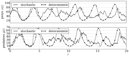
Figure 5: ‘‘Predator-pray’’ model numerical solutions (strong Runge-Kutta method)

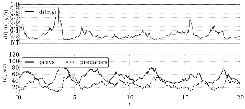
Figure 6: Invariant $\mathrm{d}I$ time evolution for process trajectory

Figure 7: Multiple trajectories (gray), $Q_{1},Q_{0}$ — percentiles and median.

Figure 8: The phase portrait of the sample means of predators and prey quantities, based on 500 trajectories obtained by Runge–Kutta method with weak convergence.

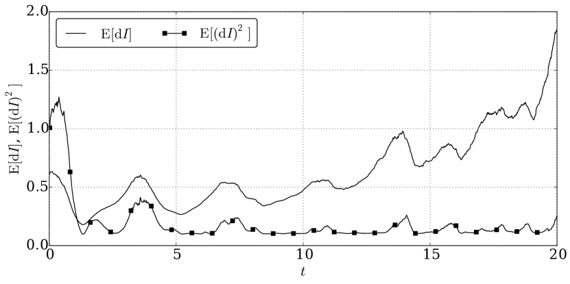
Figure 9: First and second empirical moments $\mathrm{d}I$ based on 500 trajectories obtained by Runge–Kutta method with weak convergence.

Another key difference between deterministic and stochastic models is the tendency of imminent death of population during evolution. On the fig. 7 grey colour denotes all trajectories realisations. It is seen that trajectories intersect the x-axis, thus the population of prays/predators dies. It makes stochastic model more realistic, because in the deterministic case the population death is not possible.

VI Conclusions

Some realizations of stochastic Runge-Kutta methods were considered in this article. The authors gradually developed and refined the library by adding a new functionalities and optimizing existing ones. To date, the library uses numerical methods by the Rößler’s article Rossler_2010 , as the most effective of the currently known to the authors. However, the basic functions strongSRKW1 and weakSRKp2Wm are written in accordance with the general algorithm and can use any Butcher table with appropriate staging. This allows any user of the library to extend functionality by adding new methods.

Additional examples of library usage and of all files source codes are available at https://bitbucket.org/mngev/sde-numerical-integrators. The authors suppose to maintain the library by adding new functions.

- (1) P. E. Kloeden, E. Platen, Numerical Solution of Stochastic Differential Equations, 2nd Edition, Springer, Berlin Heidelberg New York, 1995.
- (2) J. C. Butcher, Numerical Methods for Ordinary Differential Equations, 2nd Edition, Wiley, New Zealand, 2003.
- (3) E. Hairer, S. P. Nørsett, G. Wanner, Solving Ordinary Differential Equations I, 2nd Edition, Springer, Berlin, 2008.
- (4) A. Rößler, Runge-Kutta Methods for the Numerical Solution of Stochastic Differential Equations, Ph.D. thesis, Technischen Universität Darmstadt, Darmstadt (februar 2003).
- (5) K. Burrage, P. M. Burrage, High strong order explicit Runge-Kutta methods for stochastic ordinary differential equations, Appl. Numer. Math. (22) (1996) 81–101.
- (6) K. Burrage, P. M. Burrage, J. A. Belward, A bound on the maximum strong order of stochastic Runge-Kutta methods for stochastic ordinary differential equations., BIT (37) (1997) 771–780.
- (7) K. Burrage, P. M. Burrage, General order conditions for stochastic Runge-Kutta methods for both commuting and non-commuting stochastic ordinary differential equation systems, Appl. Numer. Math. (28) (1998) 161–177.
- (8) K. Burrage, P. M. Burrage, Order conditions of stochastic Runge-Kutta methods by B-series, SIAM J. Numer. Anal. (38) (2000) 1626–1646.
- (9) A. Rößler, Strong and Weak Approximation Methods for Stochastic Differential Equations – Some Recent Developments, http://www.math.uni-hamburg.de/research/papers/prst/prst2010-02.pdf (2010).
- (10) W. Stein, et al., Sage Mathematics Software (Version 6.5), The Sage Development Team, http://www.sagemath.org (2015).
- (11) A. V. Demidova, A. V. Korolkova, D. S. Kulyabov, L. A. Sevastianov, The method of stochastization of one-step processes, in: Mathematical Modeling and Computational Physics, JINR, Dubna, 2013, p. 67.
- (12) A. V. Demidova, A. V. Korolkova, D. S. Kulyabov, L. A. Sevastyanov, The method of constructing models of peer to peer protocols, in: 6th International Congress on Ultra Modern Telecommunications and Control Systems and Workshops (ICUMT), IEEE, 2014, pp. 557–562. arXiv:1504.00576, doi:10.1109/ICUMT.2014.7002162.
- (13) E. G. Eferina, A. V. Korolkova, M. N. Gevorkyan, D. S. Kulyabov, L. A. Sevastyanov, One-Step Stochastic Processes Simulation Software Package, Bulletin of Peoples’ Friendship University of Russia. Series ‘‘Mathematics. Information Sciences. Physics’’ (3) (2014) 46–59. arXiv:1503.07342.
- (14) T. R. Velieva, A. V. Korolkova, D. S. Kulyabov, Designing installations for verification of the model of active queue management discipline RED in the GNS3, in: 6th International Congress on Ultra Modern Telecommunications and Control Systems and Workshops (ICUMT), IEEE, 2014, pp. 570–577. arXiv:1504.02324, doi:10.1109/ICUMT.2014.7002164.
- (15) D. J. Higham, An algorithmic introduction to numerical simulation of stochastic differential equations, SIAM Review 43 (3) (2001) 525–546.
- (16) S. J. A. Malham, A. Wiese, An introduction to SDE simulation (2010). arXiv:1004.0646.
- (17) E. Platen, N. Bruti-Liberati, Numerical Solution of Stochastic Differential Equations with Jumps in Finance, Springer, Heidelberg Dordrecht London New York, 2010.
- (18) B. Øksendal, Stochastic differential equations. An introduction with applications, 6th Edition, Springer, Berlin Heidelberg New York, 2003.
- (19) M. Wiktorsson, Joint characteristic function and simultaneous simulation of iterated Itô integrals for multiple independent Brownian motions, The Annals of Applied Probability 11 (2) (2001) 470–487.
- (20) K. Debrabant, A. Rößler, Continuous weak approximation for stochastic differential equations, Journal of Computational and Applied Mathematics (214) (2008) 259–273.
- (21) K. Debrabant, A. Rößler, Classification of Stochastic Runge–Kutta Methods for the Weak Approximation of Stochastic Differential Equations (2013). arXiv:1303.4510.
- (22) A. Tocino, R. Ardanuy, Runge–Kutta methods for numerical solution of stochastic differential equations, Journal of Computational and Applied Mathematics (138) (2002) 219–241.
- (23) A. R. Soheili, M. Namjoo, Strong approximation of stochastic differential equations with Runge–Kutta methods, World Journal of Modelling and Simulation 4 (2) (2008) 83–93.
- (24) V. Mackevičius, Second-order weak approximations for stratonovich stochastic differential equations, Lithuanian Mathematical Journal 34 (2) (1994) 183–200. doi:10.1007/BF02333416.
- (25) G. N. Milstein, Approximate Integration of Stochastic Differential Equations, Theory Probab. Appl. (19) (1974) 557–562.
- (26) G. N. Milstein, A Method of Second-Order Accuracy Integration of Stochastic Differential Equations, Theory Probab. Appl. (23) (1979) 396–401.
- (27) G. N. Milstein, Weak Approximation of Solutions of Systems of Stochastic Differential Equations, Theory Probab. Appl. (30) (1986) 750–766.
- (28) G. Maruyama, Continuous Markov processes and stochastic equations, Rendiconti del Circolo Matematico (4) (1955) 48–90.