Strict lower bounds with separation of sources of error in non-overlapping domain decomposition methods

Abstract

This article deals with the computation of guaranteed lower bounds of the error in the framework of finite element (FE) and domain decomposition (DD) methods. In addition to a fully parallel computation, the proposed lower bounds separate the algebraic error (due to the use of a DD iterative solver) from the discretization error (due to the FE), which enables the steering of the iterative solver by the discretization error. These lower bounds are also used to improve the goal-oriented error estimation in a substructured context. Assessments on 2D static linear mechanic problems illustrate the relevance of the separation of sources of error and the lower bounds’ independence from the substructuring. We also steer the iterative solver by an objective of precision on a quantity of interest. This strategy consists in a sequence of solvings and takes advantage of adaptive remeshing and recycling of search directions.

Keywords:Verification; Error estimation; Finite element method; Domain decomposition methods; FETI; BDD

1 Introduction

Virtual testing is a useful tool for engineers to certify structures without resorting to experimental tests. However, its massive adaption comes with several challenges. Among others, virtual testing requires the capability to solve large problems (several millions degrees of freedom) and to warrant the quality of the results provided by simulations. To tackle these difficulties, we propose to use domain decomposition methods and verification. On the one hand, non-overlapping domain decomposition methods [11, 16, 7] are well-known techniques that enable the solving of large mechanical problems by exploiting parallel computers’ performance. On the other hand, verification provides tools to estimate the distance between the unknown exact solution and the computed approximated solution. This distance is the approximation error, it can be estimated by a global energy norm or by local quantities of interest (goal-oriented error estimation).

This paper is the continuation of papers connecting domain decomposition methods and verification. In [22], the authors proposed a parallel error estimator based on the error in constitutive relation [14] in a substructured framework. They described a methodology to construct the required admissible fields for error estimation. Those fields were rebuilt using quantities naturally processed during the solving and preconditioning steps of classical domain decomposition algorithms as inputs for classical equilibration techniques used in parallel on each subdomain. In [28], a new parallel error estimator that separates the discretization error (due to the finite element method) from the algebraic error (due to the iterative solver) was proposed. This new estimator enables the definition of a new stopping criterion for the iterative solver, no longer defined regardless the discretization, which avoids over-solving. Finally, in [27], this work was extended to goal-oriented error estimation. The exact value of a linear quantity of interest defined by an extractor [19, 32, 18] was estimated using global error estimation of a forward problem and an adjoint problem. It was shown that these two problems could be solved simultaneously thanks to a block-Krylov algorithm [30] steered by an objective on the error on the quantity of interest.

Upper bounds are the main concern of verification and the literature on lower bounds is scarce. By exploiting the residual equation [24] and constructing a continuous error estimation, a lower bound of the error can be computed. The question of the construction of a continuous error estimation has already been adressed in many papers (for instance [20, 4, 9]) where the authors benefit the computation of an upper bound for the computation of a lower bound.

The objective of this paper is to investigate the computation of a lower bound of the error in a substructured framework. In line with the papers associating domain decomposition methods and verification, the lower bounds are computed in parallel and they separate the two sources of error (discretization error and algebraic error). Based on the results demonstrated in [20], the computation of the lower bound does not involve significant cost since it exploits the fields computed during the reconstruction of a statically admissible stress fields.

The paper is organized as follows. In section 2, we define the reference problem and recall the principle of the error in constitutive relation. We also recall the domain decomposition methods’ principles and highlight the fields built at each iteration. Finally, we recall the parallel error estimators developed in [21, 28] and give a brief state of the art of the computation of continuous fields for lower bounds of the error. In section 3, two theorems providing lower bounds with and without separation of sources of error are demonstrated. The parallel reconstruction of fields required to compute these bounds is detailed. We also show how to benefit from this global information on the error to better the goal-oriented error estimation. In section 4, we apply these lower bounds on two-dimensional mechanical structures. We compare the lower bounds provided by a sequential approach and primal and dual approaches and also study the independence with respect to the substructuring. We illustrate the convergence of the lower bounds during the iterations and illustrate the separation of sources. Finally, in order to reach an objective of precision on a quantity of interest, we apply an auto-adaptive strategy on one of the structures. In this strategy, we use the separation of sources of error to define the stopping criterion for the iterative solver. Benefiting the informations from a first solving, we process adaptive remeshing to better the FE solution and lower the error bounds and we recycle the search directions generated (Krylov subspace recycling, see [25, 10, 29]) to speed up further solvings. Section 5 concludes the paper.

2 Settings

2.1 Reference problem

Let $\mathbb{R}^{d}$ represents the physical space. Let us consider the static equilibrium of a (polyhedral) structure which occupies the open domain $\Omega\subset\mathbb{R}^{d}$ and which is subjected to given body force $\underline{f}\in\mathtt{L}^{2}(\Omega)$ within $\Omega$, to given traction force $\underline{g}\in\mathtt{L}^{2}(\partial_{g}\Omega)$ on $\partial_{g}\Omega$ and to given displacement field $\underline{u}_{d}$ on the complementary part of the boundary (such that $\operatorname{meas}(\partial_{u}\Omega)\neq 0$). We assume that the structure undergoes small perturbations and that the material is linear elastic, characterized by Hooke’s elasticity tensor $\mathbb{H}$. Let $\underline{u}$ be the unknown displacement field, $\underline{\underline{\varepsilon}}\left(\underline{u}\right)$ the symmetric part of the gradient of $\underline{u}$, $\underline{\underline{\sigma}}$ the Cauchy stress tensor. Let $\omega$ be an open subset of $\Omega$.

We introduce two affine subspaces and one positive form:

• Affine subspace of kinematic admissible fields (KA-fields)

  $$\mathrm{KA}(\omega)=\left\{\underline{u}\in\left(\mathtt{H}^{1}(\omega)\right)^{d},\ \underline{u}=\underline{u}_{d}\text{ on }\partial\omega\bigcap\partial_{u}\Omega\right\}$$ (1)

  and we note $\mathrm{KA}^{0}(\omega)$ the following linear subspace:

  $$\mathrm{KA}^{0}(\omega)=\left\{\underline{u}\in\left(\mathtt{H}^{1}(\omega)\right)^{d},\ \underline{u}=0\text{ on }\partial\omega\bigcap\partial_{u}\Omega\right\}$$ (2)

  and $\mathrm{KA}^{00}(\omega)$ the following linear subspace:

  $$\mathrm{KA}^{00}(\omega)=\left\{\underline{u}\in\left(\mathtt{H}^{1}(\omega)\right)^{d},\ \underline{u}=0\text{ on }\partial\omega\setminus\partial_{g}\Omega\right\}$$ (3)

  Remark.

  Note that if $\omega=\Omega$, $\mathrm{KA}^{00}(\omega)$ and $\mathrm{KA}^{0}(\omega)$ are identical.

• Affine subspace of statically admissible fields (SA-fields)

  $$\mathrm{SA}(\omega)=\Bigg{\{}\underline{\underline{\tau}}\in\left(\mathtt{L}^{2}(\omega)\right)^{d\times d}_{\text{sym}};\ \forall\underline{v}\in\mathrm{KA}^{00}(\omega),\ \\ \int\limits_{\omega}\underline{\underline{\tau}}:\underline{\underline{\varepsilon}}\left(\underline{v}\right)d\Omega=\int\limits_{\omega}\underline{f}\cdot\underline{v}d\Omega+\int\limits_{\partial\omega\bigcap\partial_{g}\Omega}\underline{g}\cdot\underline{v}dS\Bigg{\}}$$ (4)

• Error in constitutive relation [14]

  $${e_{CR_{\omega}}(\underline{u},\underline{\underline{\sigma}})}=\|\underline{\underline{\sigma}}-\mathbb{H}:\underline{\underline{\varepsilon}}\left(\underline{u}\right)\|_{\mathbb{H}^{-1},\omega}$$ (5)

  where ${\|\underline{\underline{x}}\|_{\mathbb{H}^{-1},\omega}}=\displaystyle\sqrt{\int_{\omega}\left(\underline{\underline{x}}:{\mathbb{H}}^{-1}:\underline{\underline{x}}\right)d\Omega}$

The mechanical problem set on $\Omega$ can be formulated as:

$$\text{Find }\left(\underline{u}_{ex},\underline{\underline{\sigma}}_{ex}\right)\in\mathrm{KA}(\Omega)\times\mathrm{SA}(\Omega)\text{ such that }{e_{CR_{\Omega}}(\underline{u}_{ex},\underline{\underline{\sigma}}_{ex})}=0$$ (6)

The solution to this problem, named “exact” solution, exists and is unique.

Remark.

The formulation (6) is equivalent to the classical following formulation:

$$\text{Find }\underline{u}\in\mathrm{KA}(\Omega)\text{ such that }\forall\underline{v}\in\mathrm{KA}^{00}(\Omega)\text{, }a(\underline{u},\underline{v})=L(\underline{v})$$ (7)

with

$$a(\underline{u},\underline{v})=\int\limits_{\Omega}\underline{\underline{\varepsilon}}\left(\underline{u}\right):\mathbb{H}:\underline{\underline{\varepsilon}}\left(\underline{v}\right)d\Omega$$ (8)

and

$$L(\underline{v})=\int\limits_{\Omega}\underline{f}\cdot\underline{v}d\Omega+\int\limits_{\partial_{g}\Omega\bigcap\partial\Omega}\underline{g}\cdot\underline{v}dS$$ (9)

2.1.1 Finite element approximation

Let us consider a mesh of ${\Omega}$ to which we associate the finite-dimensional subspace $\mathrm{KA}_{H}(\Omega)$ of $\mathrm{KA}(\Omega)$. $\mathcal{T}$ is the set of elements of the mesh and $\mathcal{V}$ is the set of vertexes. The classical finite element displacement approximation consists in searching:

$$\underline{u}_{H} \in\mathrm{KA}_{H}(\Omega)$$ (10)

$$\underline{\underline{\sigma}}_{H} =\mathbb{H}:\underline{\underline{\varepsilon}}\left(\underline{u}_{H}\right)$$

$$\int_{\Omega}\underline{\underline{\sigma}}_{H}:\underline{\underline{\varepsilon}}\left(\underline{v}_{H}\right)d\Omega =\int_{\Omega}\underline{f}\cdot\underline{v}_{H}d\Omega+\int_{\partial_{g}\Omega}\underline{g}\cdot\underline{v}_{H}dS,\qquad\forall\underline{v}_{H}\in\mathrm{KA}^{0}_{H}(\Omega)$$

Of course the approximation is due to the fact that in most cases $\underline{\underline{\sigma}}_{H}\notin\mathrm{SA}(\Omega)$.

After introducing the matrix $\underline{\bm{\varphi}}_{H}$ of shape functions which form a basis of $\mathrm{KA}_{H}(\Omega)$ (extended to Dirichlet degrees of freedom) and the vector of nodal unknowns $\mathbf{u}$ so that $\underline{u}_{H}=\underline{\bm{\varphi}}_{H}\mathbf{u}$, the classical finite element method leads to the linear system:

$$\begin{pmatrix}\mathbf{K}_{rr}&\mathbf{K}_{rd}\\ \mathbf{K}_{dr}&\mathbf{K}_{dd}\end{pmatrix}\begin{pmatrix}\mathbf{u}_{r}\\ \mathbf{u}_{d}\end{pmatrix}=\begin{pmatrix}\mathbf{f}_{r}\\ \mathbf{f}_{d}\end{pmatrix}+\begin{pmatrix}0\\ \bm{\lambda}_{d}\end{pmatrix}$$ (11)

where $\mathbf{K}$ is the (symmetric semi positive definite) stiffness matrix and $\mathbf{f}$ is the vector of generalized forces; Subscript $d$ stands for Dirichlet degrees of freedom (where displacements are prescribed) and Subscript $r$ represents the remaining degrees of freedom so that unknowns are $\mathbf{u}_{r}$ and $\bm{\lambda}_{d}$ where Vector $\bm{\lambda}_{d}$ represents the nodal reactions:

$$\bm{\lambda}_{d}^{T}=\int_{\Omega}\underline{\underline{\sigma}}_{H}:\underline{\underline{\varepsilon}}\left({\underline{\bm{\varphi}}_{H}}_{d}\right)d\Omega-\int_{\Omega}\underline{f}\cdot{\underline{\bm{\varphi}}_{H}}_{d}d\Omega-\int_{\partial_{g}\Omega}\underline{g}\cdot{\underline{\bm{\varphi}}_{H}}_{d}dS$$ (12)

where ${\underline{\bm{\varphi}}_{H}}_{d}$ is the matrix of shape functions restricted to the Dirichlet nodes and $\underline{n}$ the outer normal vector.

2.1.2 A posteriori error estimation

Upper bound of the discretization error

The estimator we choose is based on the error in constitutive relation, which gives a guaranteed estimator for the discretization error.

The fundamental relation is the following (Prager-Synge theorem, see for instance [15]):

$$\begin{split}&\forall(\hat{\underline{u}},\hat{\underline{\underline{\sigma}}})\in\mathrm{KA}(\Omega)\times\mathrm{SA}(\Omega),\\ &\left\|\underline{\underline{\varepsilon}}\left(\underline{u}_{ex}\right)-\underline{\underline{\varepsilon}}\left(\hat{\underline{u}}\right)\right\|_{\mathbb{H},\Omega}^{2}+\left\|\underline{\underline{\sigma}}_{ex}-\hat{\underline{\underline{\sigma}}}\right\|_{\mathbb{H}^{-1},\Omega}^{2}={e^{2}_{CR_{\Omega}}(\hat{\underline{u}},\hat{\underline{\underline{\sigma}}})}\end{split}$$ (13)

We note $\vvvert\underline{v}\vvvert_{\Omega}=\left\|\underline{\underline{\varepsilon}}\left(\underline{v}\right)\right\|_{\mathbb{H},\Omega}$ the energy norm of the displacement, and since we can choose $\hat{\underline{u}}=\underline{u}_{H}\in\mathrm{KA}(\Omega)$, we retain the following upper bound for the error $\underline{{e}}_{discr}=\underline{u}_{ex}-\underline{u}_{{H}}$:

$$e_{discr}:=\vvvert\underline{{e}}_{discr}\vvvert_{\Omega}\leqslant{e_{CR_{\Omega}}({\underline{u}}_{H},\hat{\underline{\underline{\sigma}}})}$$ (14)

The construction of $\hat{\underline{\underline{\sigma}}}\in\mathrm{SA}(\Omega)$ is a complex problem solved by various approaches [14, 20, 23, 26].

The techniques [14, 23, 26] are two-steps procedures. The first step consist in building a set of equilibrated tractions or works along the edges of the elements of the mesh. Each method proposes its own strategy to reconstruct such tractions. The second step, common to all methods, is the solving of Neumann problems on each element using the equilibrated tractions as Neumann conditions.

The technique developed in [20] does not require equilibrated fluxes but only the solving local problems on star-patches (a star patch, denoted by $\omega_{i}$, is composed of the elements sharing the vertex $i$ and corresponds to the support of the shape function associated to the vertex $i$). This is the reason why the technique is sometimes called the flux-free technique.

Local problems (on element or star-patch) are usually solved on a space of finite dimension which is richer than the finite element space restrained to the support of the local problem. The space is enriched either thanks to higher degree polynomial shape functions or thanks to mesh refinement (each element being divided into several smaller elements).

Lower bound of the discretization error

A lower bound of the true error can be obtained using Cauchy-Schwarz inequality in the following residual equation:

$$\forall\underline{w}\in\mathrm{KA}^{0}(\Omega)$$ (15)

$$\int_{\Omega}\underline{\underline{\varepsilon}}\left(\underline{u}_{ex}-\underline{u}_{H}\right):\mathbb{H}:\underline{\underline{\varepsilon}}\left(\underline{w}\right)d\Omega =\int\limits_{\Omega}\underline{f}\cdot\underline{w}d\Omega+\int\limits_{\partial_{g}\Omega\bigcap\partial\Omega}\underline{g}\cdot\underline{w}dS-\int_{\Omega}\underline{\underline{\sigma}}_{H}:\underline{\underline{\varepsilon}}\left(\underline{w}\right)d\Omega$$

$$:=R_{H}(\underline{w})$$

Therefore, every displacement field $\underline{w}\in\mathrm{KA}^{0}(\Omega)\setminus\{\underline{0}\}$ can be used to obtain the following strict lower bound [24]:

$$\vvvert\underline{u}_{ex}-\underline{u}_{H}\vvvert_{\Omega}\geq\frac{|R_{H}(\underline{w})|}{\vvvert\underline{w}\vvvert_{\Omega}}$$ (16)

The accuracy of the lower bound depends on the quality of the continuous field $\underline{w}$, which is often called continuous error estimate. Indeed, the lower bound equals the true error for the continuous field $\underline{w}=\underline{u}_{ex}-\underline{u}_{H}$. The construction of $\underline{w}$ was mainly studied in [4, 20, 9] of which we recall the main results.

In [4], the error is estimated thanks to an implicit residual-based error estimator with local solvings on elements. A continuous field $\underline{w}\in\mathrm{KA}^{0}(\Omega)\setminus\{\underline{0}\}$ is constructed from the element estimators by averaging on the edges.

In [20], local problems on star-patches are solved to compute an upper bound of the error :

$$\text{Find }\underline{e}^{i}\in\mathrm{KA}^{0}(\omega_{i})\text{ such that }\forall\underline{v}\in\mathrm{KA}^{0}(\omega_{i})$$ (17)

$$a(\underline{e}^{i},\underline{v})=R_{H}(\varphi_{H}^{i}\underline{v})$$

where $\varphi_{H}^{i}$ is the shape function associated to the central node i of the star-patch. The previous problem is solved on a space $\mathrm{KA}^{0}_{h}(\omega_{i})$ richer than $\mathrm{KA}^{0}_{H}(\omega_{i})$.

The proposed continuous displacement field is:

$$\underline{w}=\Pi_{h}(\sum_{i\in\mathcal{V}}\varphi_{H}^{i}\underline{e}^{i})$$ (18)

where $\Pi_{h}$ is the projector on the space $\mathrm{KA}^{0}_{h}(\omega_{i})$. Discontinuities between star-patches vanish thanks to the multiplication by $\varphi_{H}^{i}$. The projector eases the computation of $R_{H}(\underline{w})$.

Note that in the same article, an enhanced estimate is proposed to better the lower bound :

$$\vvvert\underline{u}_{ex}-\underline{u}_{H}\vvvert^{2}_{\Omega}\geq\frac{R_{H}(\underline{w})^{2}}{\vvvert\underline{w}\vvvert^{2}_{\Omega}-\vvvert\underline{e}_{G}\vvvert^{2}_{\Omega}}$$ (19)

where $\underline{e}_{G}$ is the solution of the following global problem:

$$\text{Find }\underline{e}_{G}\in\mathrm{KA}^{0}_{H}(\Omega)\text{ such that }\forall\underline{v}\in\mathrm{KA}^{0}_{h}(\omega_{i})$$ (20)

$$a(\underline{e}_{G},\underline{v})=-a(\underline{w},\underline{v})$$

In [9], the statically admissible stress field is built from a displacement field which is the sum of the solutions of local problems on star-patches with homogeneous boundary Dirichlet conditions:

$$\text{Find }\underline{w}^{i}\in\mathrm{KA}^{0,\omega_{i}}(\omega_{i})\text{ such that }\forall\underline{v}\in\mathrm{KA}^{0,\omega_{i}}(\omega_{i})$$ (21)

$$\int_{\omega_{i}}\underline{\underline{\varepsilon}}\left(\underline{w}^{i}\right):\mathbb{H}:\underline{\underline{\varepsilon}}\left(\underline{v}\right)d\Omega=\int_{\omega_{i}}(\varphi_{i}\underline{f}-\underline{\underline{\sigma}}_{H}\underline{\operatorname{grad}}(\varphi_{i}))\underline{v}d\Omega-\int_{\omega_{i}}\varphi_{i}\underline{\underline{\sigma}}_{H}:\underline{\underline{\varepsilon}}\left(\underline{v}\right)d\Omega$$

where $\mathrm{KA}^{0,\omega_{i}}$ is the space of continuous displacement fields that equal to zero on the boundary of the star-patch $\omega_{i}$. The continuous field $\underline{w}\in\mathrm{KA}^{0}(\Omega)$ is the sum of the solutions of the previous problem:

$$\underline{w}=\sum_{i\in\mathcal{V}}\underline{w}^{i}$$ (22)

To conclude this brief review, there exist various techniques to construct $\underline{w}$. They always take advantage of the field computed during the estimation of an upper bound so that the extra-cost is very limited.

2.1.3 Substructured formulation

Let us consider a decomposition of domain $\Omega$ in $N_{sd}$ regular open subsets $(\Omega^{(s)})_{s}$ such that $\Omega^{(s)}\bigcap\Omega^{(s^{\prime})}=\emptyset$ for $s\neq s^{\prime}$ and $\bar{\Omega}=\bigcup_{s}\bar{\Omega}^{(s)}$. We note $\partial_{g}\Omega^{(s)}=\partial\Omega^{(s)}\bigcap\partial_{g}\Omega$ the Neumann border of subdomains.

The mechanical problem on the substructured configuration writes :

$$\forall s\left\{\begin{aligned} &\underline{u}^{(s)}\in\mathrm{KA}(\Omega^{(s)})\\ &\underline{\underline{\sigma}}^{(s)}\in\mathrm{SA}(\Omega^{(s)})\\ &{e_{CR_{\Omega^{(s)}}}(\underline{u}^{(s)},\underline{\underline{\sigma}}^{(s)})}=0\end{aligned}\right.$$ (23)

and

$${\forall(s,s^{\prime})\text{ such that }\Omega^{(s)}\text{ and }\Omega^{(s^{\prime})}\text{ are adjacent }}\left\{\begin{aligned} &\operatorname{tr}(\underline{u}^{(s)})=\operatorname{tr}(\underline{u}^{(s^{\prime})})\text{ on }\Gamma^{(s,s^{\prime})}\\ &\underline{\underline{\sigma}}^{(s)}\cdot\underline{n}^{(s)}+\underline{\underline{\sigma}}^{(s^{\prime})}\cdot\underline{n}^{(s^{\prime})}=\underline{0}\text{ on }\Gamma^{(s,s^{\prime})}\end{aligned}\right.$$ (24)

The set of fields $\underline{u}$ defined on $\Omega$ such that $\underline{u}_{|\Omega^{(s)}}\in\mathrm{KA}(\Omega^{(s)})$ without interface continuity is a broken space which we note $\mathrm{KA}(\bigcup\Omega^{(s)})$.

2.1.4 Finite element approximation for the substructured problem

We assume that the mesh of $\bar{\Omega}$ and the substructuring are conforming. This hypothesis implies that each element only belongs to one subdomain and nodes are matching on the interfaces. For each subdomain, let us denote by the subscript b the degrees of freedom on the boundary of the subdomain and by the subscript i the degrees of fredom inside the subdomain.

Let $\mathbf{t}^{(s)}$ be the discrete trace operator on the interface. $\mathbf{t}^{(s)}$ enables to cast degrees of freedom from a complete subdomain to its interface. Using an adapted ordering, we have

$$\mathbf{t}^{(s)}=\begin{pmatrix}\mathbf{{I}}_{bb}&\mathbf{0}_{bi}\end{pmatrix}$$ (25)

Therefore ${\mathbf{t}^{(s)}}^{T}$ is the extension by zero operator: it extends data supported by the boundary to the whole subdomain.

Let us introduce the unknown nodal reaction on the interface $\bm{\lambda}^{(s)}$, the equilibrium of each subdomain writes:

$$\mathbf{K}^{(s)}\mathbf{u}^{(s)}=\mathbf{f}^{(s)}+{\mathbf{t}^{(s)}}^{T}\bm{\lambda}^{(s)}$$ (26)

Let $(\mathbf{A}^{(s)})$ and $(\mathbf{B}^{(s)})$ be the primal and dual assembly operator. Those operators are signed boolean operators. The dual operator $(\mathbf{B}^{(s)})$ enables to express the continuity of displacements and the primal operator $(\mathbf{A}^{(s)})$ enables to express the mechanical equilibrium of interface. Their number of columns is equal to the number of boundary degrees of freedom. $\mathbf{A}^{(s)}$ injects the boundary degrees of freedom of $\Omega^{(s)}$ in the global interface. Thus the number of rows of $\mathbf{A}^{(s)}$ is equal to the number of degrees of freedom on the global interface. The number of rows of $\mathbf{B}^{(s)}$ is equal to the number of connections between pairs of neighboring degrees of freedom.

In the case of two subdomains, we have $\sum_{s}\mathbf{B}^{(s)}\mathbf{t}^{(s)}\mathbf{u}^{(s)}=\mathbf{t}^{(1)}\mathbf{u}^{(1)}-\mathbf{t}^{(2)}\mathbf{u}^{(2)}$ and $\sum_{s}\mathbf{A}^{(s)}\bm{\lambda}^{(s)}~{}=~{}\bm{\lambda}^{(1)}+\bm{\lambda}^{(2)}$. For more details on the assembly operators, the reader can refer to [11].

The discrete counterpart of the interface admissibility equations is:

$$\left\{\begin{aligned} \sum_{s}\mathbf{B}^{(s)}\mathbf{t}^{(s)}\mathbf{u}^{(s)}&=0\\ \sum_{s}\mathbf{A}^{(s)}\bm{\lambda}^{(s)}&=0\\ \end{aligned}\right.$$ (27)

Equations (26) and (27) form the discrete substructured system, which is equivalent to the global problem (11).

2.1.5 Domain decomposition solvers and admissible fields

Domain decomposition solvers are well described in many papers (see for instance [11] and the associated bibliography). The principle is to condense the global problem on the interface to create a smaller problem. In classical algorithms such as BDD [16] and FETI [7], this new interface problem is solved iteratively thanks to a projected preconditioned conjugate gradient. Each iteration implies two parallel solvings on subdomains with two dual operators (one for the preconditioning step, one for the direct step) so that local problems with Neumann boundary conditions and local problems with Dirichlet boundary conditions are alternatively solved. In [22] it was proved that the following fields could be processed at no extra cost:

• $(\underline{u}_{D}^{(s)})_{s}\in\mathrm{KA}(\Omega)$: displacement field which results from a Dirichlet problem and which is thus globally admissible

• $(\bm{\lambda}_{N}^{(s)})_{s}$ : nodal reactions which are balanced at the interface.

• $(\underline{u}_{N}^{(s)})_{s}\in\mathrm{KA}(\bigcup\Omega^{(s)})$: displacement field which results from a Neumann problem and which is not globally admissible

• $\underline{\underline{\sigma}}_{N}^{(s)}$: the stress field associated to $\underline{u}_{N}^{(s)}$ ($\underline{\underline{\sigma}}_{N}^{(s)}=\mathbb{H}:\underline{\underline{\varepsilon}}\left(\underline{u}_{N}^{(s)}\right)$). It can be used (with additional input $\bm{\lambda}_{N}^{(s)}$) to build in parallel stress fields $\hat{\underline{\underline{\sigma}}}_{N}^{(s)}$ which are statically admissible $\hat{\underline{\underline{\sigma}}}_{N}=(\hat{\underline{\underline{\sigma}}}_{N}^{(s)})_{s}\in\mathrm{SA}(\Omega)$ using dedicated methods such as [14, 20, 23, 26].

In [28] we proved the following result where $\alpha$ (denoted $\sqrt{\mathbf{r}^{T}\mathbf{z}}$ in [28]) is the preconditioner-norm of the residual, a quantity that is actually computed by the solver:

$$\alpha:=\lVert\underline{u}_{N}-\underline{u}_{D}\rVert_{\mathbb{H},\Omega}=\sqrt{\mathbf{r}^{T}\mathbf{z}}$$ (28)

2.2 A posteriori upper bound of the error in substructured context

In [22], a first parallel error estimator in substructured context was introduced. It is based on the error in constitutive relation and reads :

$$\vvvert\underline{u}_{ex}-\underline{u}_{D}\vvvert_{\Omega}=\sqrt{\sum_{s}\vvvert\underline{u}_{ex}^{(s)}-\underline{u}_{D}^{(s)}\vvvert_{\Omega^{(s)}}^{2}}\leqslant\sqrt{\sum_{s}{e^{2}_{CR_{\Omega^{(s)}}}(\underline{u}_{D}^{(s)},\hat{\underline{\underline{\sigma}}}_{N}^{(s)})}}$$ (29)

In [28], we showed that this estimator mixes two different sources of error : the discretization error which is inherent to the use of the finite element method and the algebraic error which is due to the use of an iterative solver which would not exist for a direct solver. The algebraic error monitors the convergence of the solver and can be made as small as wished. Therefore, a second parallel error estimator was proposed in [28]:

$$\vvvert\underline{u}_{ex}-\underline{u}_{N}\vvvert_{\Omega}\leq\alpha+\sqrt{\sum_{s}{e^{2}_{CR_{\Omega^{(s)}}}(\underline{u}_{N}^{(s)},\hat{\underline{\underline{\sigma}}}_{N}^{(s)})}}$$ (30)

$$\vvvert\underline{u}_{ex}-\underline{u}_{D}\vvvert_{\Omega}\leq\alpha+\sqrt{\sum_{s}{e^{2}_{CR_{\Omega^{(s)}}}(\underline{u}_{N}^{(s)},\hat{\underline{\underline{\sigma}}}_{N}^{(s)})}}$$ (31)

This estimator separates the two sources of error. When the solver has converged the two displacements fields $\underline{u}_{N}$ and $\underline{u}_{D}$ are identical and equal to $\underline{u}_{H}$ (the algebraic error $\alpha$ is very close to zero). $\sqrt{\sum_{s}{e^{2}_{CR_{\Omega^{(s)}}}(\underline{u}_{N}^{(s)},\hat{\underline{\underline{\sigma}}}_{N}^{(s)})}}$ is the estimation of the discretization error. As a consequence, at convergence, the estimators (29), (30) and (31) are identical.

3 Lower bound of the error in substructured context

In this section, we extend sequential results to demonstrate guaranteed lower bounds of the error in substructured context. Moreover, we prove a theorem that enables the separation of sources of error in the lower bound. We also develop the methodology to build a continuous error estimate from parallel error estimation procedure. Finally, we extend those results to goal-oriented error estimation.

3.1 A first lower bound of the error

Theorem 1.

Let $\underline{u}_{ex}\in\mathrm{KA}(\Omega)$ be the exact solution, $(\underline{u}_{D}^{(s)})_{s}\in\mathrm{KA}(\Omega)$ the displacement field defined in 2.1.5 and $\underline{w}\in\mathrm{KA}^{0}(\Omega)\setminus\{\underline{0}\}$ then

$$\vvvert\underline{u}_{ex}-\underline{u}_{D}\vvvert_{\Omega}\geq\frac{|{R}_{D}(\underline{w})|}{\sqrt{\sum_{s}\vvvert\underline{w}^{(s)}\vvvert_{\Omega^{(s)}}^{2}}}$$ (32)

with

$${R}_{D}(\underline{w}) =\sum_{s}R_{D}^{(s)}(\underline{w}^{(s)})$$ (33)

$${R}_{D}^{(s)}(\underline{w}^{(s)}) :=\int\limits_{\Omega^{(s)}}\underline{f}\cdot\underline{w}^{(s)}d\Omega+\int\limits_{\partial_{g}\Omega^{(s)}}\underline{g}\cdot\underline{w}^{(s)}dS-\int\limits_{\Omega^{(s)}}\underline{\underline{\varepsilon}}\left(\underline{u}_{D}^{(s)}\right):\mathbb{H}:\underline{\underline{\varepsilon}}\left(\underline{w}^{(s)}\right)d{\Omega^{(s)}}$$ (34)

Proof.

This property is the direct application of (16) where we replace the displacement field $\underline{u}_{H}\in\mathrm{KA}(\Omega)$ by $(\underline{u}_{D}^{(s)})_{s}\in\mathrm{KA}(\Omega)$. The residual $R_{D}(\underline{w})$ can be rewritten:

$$R_{D}(\underline{w}) =\sum_{s}R_{D}^{(s)}(\underline{w}^{(s)})$$ (35)

$$=\sum_{s}\left(\int\limits_{\Omega^{(s)}}\underline{f}\cdot\underline{w}^{(s)}d\Omega+\int\limits_{\partial_{g}\Omega^{(s)}}\underline{g}\cdot\underline{w}^{(s)}dS-\int\limits_{\Omega^{(s)}}\underline{\underline{\varepsilon}}\left(\underline{u}_{D}^{(s)}\right):\mathbb{H}:\underline{\underline{\varepsilon}}\left(\underline{w}^{(s)}\right)d{\Omega^{(s)}}\right)$$

$$=L(\underline{w})-a(\underline{u}_{D},\underline{w})$$

∎

In practice, we choose $\underline{w}^{(s)}\in\mathrm{KA}^{00}(\Omega^{(s)})\setminus\{\underline{0}\}\subset\mathrm{KA}^{0}(\Omega)\setminus\{\underline{0}\}$, which corresponds to imposing the nullity along the interface and which is inexpensive since it does not imply exchanges between subdomains. In subsection 3.3, we will give details about the computation of $\underline{w}$. Therefore the computation of a lower bound is as parallel as for the upper bound. In the assessments in section 4, we will verify that this lower bound is as accurate as the one obtained in the sequential context and that the quality neither depends on the approach (primal or dual) nor on the substructuring. Moreover, this lower bound is computable whatever the state of the iterative solver (converged or not).

3.2 Lower bound with separation of sources of error

Continuing the philosophy of separating the sources of error as detailed in [28], we propose a second lower bound :

Theorem 2.

Let $\underline{u}_{ex}\in\mathrm{KA}(\Omega)$ be the exact solution, $(\underline{u}_{D}^{(s)})_{s}\in\mathrm{KA}(\Omega)$ and $(\underline{u}_{N}^{(s)})_{s}\in\mathrm{KA}(\bigcup\Omega^{(s)})$ the displacement fields defined in 2.1.5 and $\underline{w}\in\mathrm{KA}^{0}(\Omega)\setminus\{\underline{0}\}$ , then

$$\vvvert\underline{u}_{ex}-\underline{u}_{D}\vvvert_{\Omega}\geq\left|\frac{|{R}_{N}(\underline{w})|}{\sqrt{\sum_{s}\vvvert\underline{w}^{(s)}\vvvert_{\Omega^{(s)}}^{2}}}-\frac{|a(\underline{u}_{D}-\underline{u}_{N},\underline{w})|}{\sqrt{\sum_{s}\vvvert\underline{w}^{(s)}\vvvert_{\Omega^{(s)}}^{2}}}\right|$$ (36)

which leads to the coarser bound

$$\vvvert\underline{u}_{ex}-\underline{u}_{D}\vvvert_{\Omega}\geq\frac{|R_{N}(\underline{w})|}{\sqrt{\sum_{s}\vvvert\underline{w}^{(s)}\vvvert_{\Omega^{(s)}}^{2}}}-\alpha$$ (37)

with

$${R}_{N}(\underline{w}) =\sum_{s}R_{N}^{(s)}(\underline{w}^{(s)})$$ (38)

$${R}_{N}^{(s)}(\underline{w}^{(s)}) :=\int\limits_{\Omega^{(s)}}\underline{f}\cdot\underline{w}^{(s)}d\Omega+\int\limits_{\partial_{g}\Omega^{(s)}}\underline{g}\cdot\underline{w}^{(s)}dS-\int\limits_{\Omega^{(s)}}\underline{\underline{\varepsilon}}\left(\underline{u}_{N}^{(s)}\right):\mathbb{H}:\underline{\underline{\varepsilon}}\left(\underline{w}^{(s)}\right)d{\Omega^{(s)}}$$ (39)

Proof.

The proof of the first inequality is based on theorem 1 and on the triangle inequality :

$$\vvvert\underline{u}_{ex}-\underline{u}_{D}\vvvert_{\Omega} \geq\frac{|{R}_{D}(\underline{w})|}{\sqrt{\sum_{s}\vvvert\underline{w}^{(s)}\vvvert_{\Omega^{(s)}}^{2}}}$$ (40)

$$\vvvert\underline{u}_{ex}-\underline{u}_{D}\vvvert_{\Omega} \geq\frac{|L(\underline{w})-a(\underline{u}_{D},\underline{w})|}{\sqrt{\sum_{s}\vvvert\underline{w}^{(s)}\vvvert_{\Omega^{(s)}}^{2}}}$$

$$\geq\frac{|L(\underline{w})-a(\underline{u}_{N},\underline{w})-a(\underline{u}_{D}-\underline{u}_{N},\underline{w})|}{\sqrt{\sum_{s}\vvvert\underline{w}^{(s)}\vvvert_{\Omega^{(s)}}^{2}}}$$

$$\geq\left|\frac{|{R}_{N}(\underline{w})|}{\sqrt{\sum_{s}\vvvert\underline{w}^{(s)}\vvvert_{\Omega^{(s)}}^{2}}}-\frac{|a(\underline{u}_{D}-\underline{u}_{N},\underline{w})|}{\sqrt{\sum_{s}\vvvert\underline{w}^{(s)}\vvvert_{\Omega^{(s)}}^{2}}}\right|$$

which proves (36). (37) is simply based on the remark that

$$\left|\frac{|R_{N}(\underline{w})|}{\sqrt{\sum_{s}\vvvert\underline{w}^{(s)}\vvvert_{\Omega^{(s)}}^{2}}}-\frac{|a(\underline{u}_{D}-\underline{u}_{N},\underline{w})|}{\sqrt{\sum_{s}\vvvert\underline{w}^{(s)}\vvvert_{\Omega^{(s)}}^{2}}}\right|\geq\frac{|R_{N}(\underline{w})|}{\sqrt{\sum_{s}\vvvert\underline{w}^{(s)}\vvvert_{\Omega^{(s)}}^{2}}}-\frac{|a(\underline{u}_{D}-\underline{u}_{N},\underline{w})|}{\sqrt{\sum_{s}\vvvert\underline{w}^{(s)}\vvvert_{\Omega^{(s)}}^{2}}}$$ (41)

and using twice the Cauchy-Schwarz inequality, we have :

$$|a(\underline{u}_{D}-\underline{u}_{N},\underline{w})| =|\sum_{s}\int_{\Omega^{(s)}}\underline{\underline{\varepsilon}}\left(\underline{u}_{D}^{(s)}-\underline{u}_{N}^{(s)}\right):\mathbb{H}:\underline{\underline{\varepsilon}}\left(\underline{w}^{(s)}\right)|$$ (42)

$$\leq\sum_{s}\vvvert\underline{u}_{N}^{(s)}-\underline{u}_{D}^{(s)}\vvvert_{\Omega^{(s)}}\vvvert\underline{w}^{(s)}\vvvert_{\Omega^{(s)}}$$

$$\leq\sqrt{\sum_{s}\vvvert\underline{u}_{N}^{(s)}-\underline{u}_{D}^{(s)}\vvvert^{2}_{\Omega^{(s)}}}\sqrt{\sum_{s}\vvvert\underline{w}^{(s)}\vvvert^{2}_{\Omega^{(s)}}}$$

Finally, using the equality (28):

$$\vvvert\underline{u}_{ex}-\underline{u}_{D}\vvvert_{\Omega}\geq\frac{|R_{N}(\underline{w})|}{\sqrt{\sum_{s}\vvvert\underline{w}^{(s)}\vvvert_{\Omega^{(s)}}^{2}}}-\alpha$$ (43)

∎

As said earlier, the term $\alpha$ is a measure of the residual so it is purely algebraic whereas the first term of the inequality is mainly driven by the discretization error. During the first iterations, the second lower bound is not accurate because the algebraic error prevails so that $\frac{|L(\underline{w})-a(\underline{u}_{N},\underline{w})|}{\sqrt{\sum_{s}\vvvert\underline{w}^{(s)}\vvvert_{\Omega^{(s)}}^{2}}}-\alpha$ is negative and it is a trivial lower bound of the positive true error $\vvvert\underline{u}_{ex}-\underline{u}_{D}\vvvert_{\Omega}$. When the solver reaches convergence, the three lower bounds in theorems 1 and 2 are identical.

3.3 Reconstruction of admissible field $\underline{w}$

The upper bounds of the error (30) or (31) require the construction of a statically admissible field $(\hat{\underline{\underline{\sigma}}}_{N}^{(s)})_{s}$. In case the flux-free technique is chosen, it is possible to construct a continuous field $\underline{w}^{(s)}\in\mathrm{KA}^{00}(\Omega^{(s)})$ using the methodology developed in [20] for each subdomain in parallel. As a consequence,

$$\left((\Pi_{h}(\sum_{i\in\mathcal{V}}\phi_{H}^{i}\underline{e}^{i}))^{(s)}\right)_{s}\in\mathrm{KA}(\bigcup\Omega^{(s)})$$ (44)

In order to have $\underline{w}^{(s)}\in\mathrm{KA}^{00}(\Omega^{(s)})$, we choose not to sum the contributions from the nodes located on the interface of the subdomain $(s)$. They will be denoted as $\mathcal{V}_{\Gamma}$. $\underline{w}^{(s)}$ is defined by :

$$\underline{w}^{(s)}=(\Pi_{h}(\sum_{i\in\mathcal{V}\setminus\mathcal{V}_{\Gamma}}\varphi_{H}^{i}\underline{e}^{i}))^{(s)}$$ (45)

Therefore $\underline{w}^{(s)}\in\mathrm{KA}^{00}(\Omega^{(s)})$ and $\underline{w}=(\underline{w}^{(s)})_{s}\in\mathrm{KA}^{0}(\Omega)$.

Remark.

Using the subtle trick in [20], the computation of the discretized fields is eased. Indeed:

$$\mathbf{w}^{(s)}=\sum_{i\in\mathcal{V}\setminus\mathcal{V}_{\Gamma}}{\mathbf{\bm{\varphi}_{H}^{i}}}\odot\mathbf{{e}^{i}}^{(s)}$$ (46)

and

$$\mathbf{R_{D}}^{(s)}(\mathbf{w}^{(s)})\\ =\sum_{i\in\mathcal{V}-\mathcal{V}_{\Gamma}}{\mathbf{\bm{\varphi}_{H}^{i}}}\odot\mathbf{R_{D}}^{(s)}(\mathbf{{e}^{i}}^{(s)})$$ (47)

where $\mathbf{\bm{\varphi}_{H}^{i}}$ gathers the nodal values of the shape function $\varphi_{H}^{i}$ projected on the richer space used to solve the star-patch problem whose $\mathbf{{e}^{i}}^{(s)}$ is the discretized solution and where $\odot$ represents the term by term multiplication.

Remark.

If the method chosen to construct the admissible field is based on elements problems [4], it is always possible to construct a displacement field $\underline{w}^{(s)}\in\mathrm{KA}^{00}(\Omega^{(s)})$ by computing the mean value along the edges inside the subdomains and imposing zero along the interfaces between subdomains.

3.4 Goal-oriented error estimation

Goal-oriented error estimation offers the possibility to have upper and lower bounds of the unknown exact value of a quantity of interest. Among various techniques, extractors (see [1] for instance) are the most common tools to define linear quantities of interest. They lead to the definition and the solving of an adjoint problem.

3.4.1 Definition of the linear quantity of interest and of the adjoint problem

Let $\widetilde{L}$ be the linear functional defining the quantity of interest $I$:

$$I=\widetilde{L}(\underline{u})=\int_{\Omega}(\underline{\underline{\sigma}}_{\Sigma}:\underline{\underline{\varepsilon}}\left(\underline{u}\right)+\underline{f}_{\Sigma}\underline{u})d\Omega$$ (48)

where $\underline{\underline{\sigma}}_{\Sigma}$ and $\underline{f}_{\Sigma}$ are extractors.

We introduce the affine subspace of statically admissible fields (adjoint SA-fields) for the adjoint problem:

$$\widetilde{\mathrm{SA}}(\omega)=\Bigg{\{}\underline{\underline{\tau}}\in\left(\mathtt{L}^{2}(\omega)\right)^{d\times d}_{\text{sym}};\ \forall\underline{v}\in\mathrm{KA}^{00}(\omega),\ \int\limits_{\omega}\underline{\underline{\tau}}:\underline{\underline{\varepsilon}}\left(\underline{v}\right)d\omega=\tilde{L}(\underline{v})\Bigg{\}}$$ (49)

The adjoint problem set on $\Omega$ can be formulated as:

$$\text{Find }\left(\underline{\widetilde{u}}_{ex},\underline{\underline{\widetilde{\sigma}}}_{ex}\right)\in\mathrm{KA}^{0}(\Omega)\times\widetilde{\mathrm{SA}}(\Omega)\text{ such that }{e_{CR_{\Omega}}(\underline{\widetilde{u}}_{ex},\underline{\underline{\widetilde{\sigma}}}_{ex})}=0$$ (50)

The solution to this problem, named exact solution, exists and is unique.

Remark.

The formulation (50) is equivalent to the classical following formulation:

$$\text{Find }\underline{\widetilde{u}}_{ex}\in\mathrm{KA}^{0}(\Omega)\text{ such that }\forall\underline{v}\in\mathrm{KA}^{0}(\Omega)\text{, }a(\underline{\widetilde{u}}_{ex},\underline{v})=\widetilde{L}(\underline{v})$$ (51)

where a is the classical bilinear form (8).

The adjoint problem is usually solved with the finite element method. The mesh can differ from the one used for the forward problem. The approximated adjoint displacement is ${\underline{\widetilde{u}}}_{\widetilde{H}}$.

The discretization error for the adjoint problem is

$$e_{discr}=\vvvert\underline{\widetilde{e}}_{discr}\vvvert_{\Omega}=\vvvert\underline{\widetilde{u}}_{ex}-\underline{\widetilde{u}}_{\widetilde{H}}\vvvert_{\Omega}$$ (52)

3.4.2 Error estimation of quantities of interest

As said earlier the adjoint problem is meant to extract one quantity of interest in the forward problem. Let $I_{ex}=\tilde{L}(\underline{u}_{ex})$ be the unknown exact value of the quantity of interest. $I_{H}=\tilde{L}({\underline{u}}_{D})$ is an approximation of this quantity of interest.

A bounding of the exact value of the quantity of interest $I_{ex}$ is [12, 13]:

$$\arrowvert I_{ex}-I_{H}-I_{HH2}\arrowvert\leq\frac{1}{2}{e_{CR_{\Omega}}(\underline{u}_{H},\hat{\underline{\underline{\sigma}}}_{H})}{e_{CR_{\Omega}}({\underline{\widetilde{u}}}_{\widetilde{H}},\hat{\underline{\underline{\widetilde{\sigma}}}}_{\widetilde{H}})}$$ (53)

where

$$I_{HH2}=\int\limits_{\Omega}\frac{1}{2}(\hat{\underline{\underline{\widetilde{\sigma}}}}_{\widetilde{H}}+\mathbb{H}:\underline{\underline{\varepsilon}}\left(\underline{\widetilde{u}}_{\widetilde{H}}\right)):\mathbb{H}^{-1}:(\hat{\underline{\underline{\sigma}}}_{H}-\mathbb{H}:\underline{\underline{\varepsilon}}\left(\underline{u}_{H}\right))d\Omega$$ (54)

and where $\hat{\underline{\underline{\widetilde{\sigma}}}}_{\widetilde{H}}\in\widetilde{\mathrm{SA}}_{H}(\Omega)$.

The error on the quantity of interest can also be estimated using the parallelogram identity [24]:

$$\left\{\begin{aligned} I_{ex}-I_{H}=\widetilde{L}(\underline{e}_{discr})&=a(\underline{e}_{discr},\underline{\widetilde{e}}_{discr})\\ &=a(\kappa\underline{e}_{discr},\frac{1}{\kappa}\underline{\widetilde{e}}_{discr})\\ &=\frac{1}{4}[\vvvert{{\kappa\underline{e}_{discr}+\frac{1}{\kappa}\underline{\widetilde{e}}_{discr}}}\vvvert^{2}_{\Omega}-\vvvert{\kappa\underline{e}_{discr}-\frac{1}{\kappa}\underline{\widetilde{e}}_{discr}}\vvvert^{2}_{\Omega}]\\ \end{aligned}\right.$$ (55)

where $\kappa$ is a scalar parameter whose optimal value is:

$$\kappa=\frac{{e_{CR_{\Omega}}({\underline{\widetilde{u}}}_{H},\hat{\underline{\underline{\widetilde{\sigma}}}}_{H})}}{{e_{CR_{\Omega}}(\underline{u}_{H},\hat{\underline{\underline{\sigma}}}_{H})}}$$ (56)

This optimal value minimizes the difference and thus improves the quality of the bounding. Introducing upper and lower bounds:

$$\beta^{+}_{inf} \leq\vvvert\kappa\underline{e}_{discr}+\frac{1}{\kappa}\underline{\widetilde{e}}_{discr}\vvvert_{\Omega}^{2}\leq\beta^{+}_{sup}$$ (57)

$$\beta^{-}_{inf} \leq\vvvert\kappa\underline{e}_{discr}-\frac{1}{\kappa}\underline{\widetilde{e}}_{discr}\vvvert_{\Omega}^{2}\leq\beta^{-}_{sup}$$

it is possible to obtain lower and upper bounds of the error on the quantity of interest :

$$\frac{1}{4}\beta^{+}_{inf}-\frac{1}{4}\beta^{-}_{sup}\leq I_{ex}-I_{H}\leq\frac{1}{4}\beta^{+}_{sup}-\frac{1}{4}\beta^{-}_{inf}$$ (58)

3.4.3 Application to the substructured context

Let us suppose that the forward and adjoint problems are solved on the same mesh and on the same substructuring. Since the two problems share the same stiffness matrices on every subdomain, they can be solved simultaneously using a block algorithm. Following the same methodology described in section 2.1.5, one can compute the following admissible fields for the adjoint problem:

• $(\underline{\widetilde{u}}_{D}^{(s)})_{s}\in\mathrm{KA}^{0}(\Omega)$: displacement field which results from a Dirichlet problem and which is thus globally admissible

• $\widetilde{\bm{\lambda}}_{N}^{(s)}$ : nodal reactions which are balanced at the interface.

• $(\underline{\widetilde{u}}_{N}^{(s)})_{s}\in\mathrm{KA}(\bigcup\Omega^{(s)})$: displacement field which results from a Neumann problem and which is not globally admissible

• $\underline{\underline{\widetilde{\sigma}}}_{N}^{(s)}$: stress field associated to $\underline{\widetilde{u}}_{N}^{(s)}$ ($\underline{\underline{\widetilde{\sigma}}}_{N}^{(s)}=\mathbb{H}:\underline{\underline{\varepsilon}}\left(\underline{\widetilde{u}}_{N}^{(s)}\right)$). It can be used (with additional input $\widetilde{\bm{\lambda}}_{N}^{(s)}$) to build in parallel stress fields $\hat{\underline{\underline{\widetilde{\sigma}}}}_{N}^{(s)}$ which are statically admissible $\hat{\underline{\underline{\widetilde{\sigma}}}}_{N}=(\hat{\underline{\underline{\widetilde{\sigma}}}}_{N}^{(s)})_{s}\in\widetilde{\mathrm{SA}}(\Omega)$.

We also have the equality that expresses the distance between the Neumann and Dirichlet displacement fields in terms of the algebraic residual $\widetilde{\alpha}$ of the adjoint problem :

$$\lVert\underline{\widetilde{u}}_{N}-\underline{\widetilde{u}}_{D}\rVert_{\mathbb{H},\Omega}=\widetilde{\alpha}$$ (59)

For more details about the computation of those fields, the reader can refer to [27].

The upper bounds of the global error presented in section 2.2 and the lower bound in the theorem 1 can be applied on the adjoint problem.

Upper and lower bounds for goal-oriented error estimation

We demonstrate two properties that give upper and lower bounds of the terms in the parallelogram identity. The properties are merely the application of the results on goal-oriented error estimation [12, 13, 20] into a substructured context.

Corollary 1.

Using notations of paragraph 2.1.5 and 3.4.3

$$\beta^{+}_{inf}\leq{\vvvert\kappa\underline{e}_{discr}+\frac{1}{\kappa}\underline{\widetilde{e}}_{discr}\vvvert_{\Omega}}^{2}\leq\beta^{+}_{sup}$$ (60)

$$\beta^{-}_{inf}\leq{\vvvert\kappa\underline{e}_{discr}-\frac{1}{\kappa}\underline{\widetilde{e}}_{discr}\vvvert_{\Omega}}^{2}\leq\beta^{-}_{sup}$$

with

$$\left\{\begin{aligned} \beta^{+}_{sup}&=2\sqrt{\sum_{s}{e_{CR_{\Omega^{(s)}}}(\underline{u}_{D}^{(s)},\hat{\underline{\underline{\sigma}}}_{N}^{(s)})}^{2}}\sqrt{\sum_{s}{e_{CR_{\Omega^{(s)}}}({\underline{\widetilde{u}}}_{D}^{(s)},\hat{\underline{\underline{\widetilde{\sigma}}}}_{N}^{(s)})}^{2}}\\ &+2\sum_{s}\int_{\Omega^{(s)}}(\hat{\underline{\underline{\widetilde{\sigma}}}}^{(s)}_{N}-\mathbb{H}\underline{\underline{\varepsilon}}\left(\underline{\widetilde{u}}^{(s)}_{D}\right)):\mathbb{H}^{-1}:(\hat{\underline{\underline{\sigma}}}^{(s)}_{N}-\mathbb{H}:\underline{\underline{\varepsilon}}\left(\underline{u}_{D}^{(s)}\right))d\Omega\\ \beta^{+}_{inf}&=\frac{(\kappa{R_{D}}(\underline{z}^{+})+\frac{1}{\kappa}\widetilde{{R}}_{D}(\underline{z}^{+}))^{2}}{{\sum_{s}\vvvert(\underline{z}^{+})^{(s)}\vvvert^{2}_{\Omega^{(s)}}}}\\ &\text{ with }(\underline{z}^{+})^{(s)}=\kappa\underline{w}^{(s)}+\frac{1}{\kappa}\underline{\widetilde{w}}^{(s)}\end{aligned}\right.$$ (61)

and

$$\left\{\begin{aligned} \beta^{-}_{sup}&=2\sqrt{\sum_{s}{e_{CR_{\Omega^{(s)}}}(\underline{u}_{D}^{(s)},\hat{\underline{\underline{\sigma}}}_{N}^{(s)})}^{2}}\sqrt{\sum_{s}{e_{CR_{\Omega^{(s)}}}({\underline{\widetilde{u}}}_{D}^{(s)},\hat{\underline{\underline{\widetilde{\sigma}}}}_{N}^{(s)})}^{2}}\\ &-2\sum_{s}\int_{\Omega^{(s)}}(\hat{\underline{\underline{\widetilde{\sigma}}}}^{(s)}_{N}-\mathbb{H}\underline{\underline{\varepsilon}}\left(\underline{\widetilde{u}}^{(s)}_{D}\right)):\mathbb{H}^{-1}:(\hat{\underline{\underline{\sigma}}}^{(s)}_{N}-\mathbb{H}:\underline{\underline{\varepsilon}}\left(\underline{u}_{D}^{(s)}\right))d\Omega\\ \beta^{-}_{inf}&=\frac{(\kappa{R_{D}}(\underline{z}^{-})-\frac{1}{\kappa}\widetilde{{R}}_{D}(\underline{z}^{-}))^{2}}{{\sum_{s}\vvvert(\underline{z}^{-})^{(s)}\vvvert^{2}_{\Omega^{(s)}}}}\\ &\text{ with }(\underline{z}^{-})^{(s)}=\kappa\underline{w}^{(s)}-\frac{1}{\kappa}\underline{\widetilde{w}}^{(s)}\end{aligned}\right.$$ (62)

One has to pay attention to the computation of the parameter $\kappa$ which implies exchanges between subdomains. Indeed, this coefficient is defined by:

$$\kappa=\frac{\sqrt{\sum_{s}{e_{CR_{\Omega^{(s)}}}({\underline{\widetilde{u}}}_{D}^{(s)},\hat{\underline{\underline{\widetilde{\sigma}}}}_{N}^{(s)})}}}{\sqrt{\sum_{s}{e_{CR_{\Omega^{(s)}}}(\underline{u}_{D}^{(s)},\hat{\underline{\underline{\sigma}}}_{N}^{(s)})}}}$$ (63)

Anyhow this exchange between subdomains is already done at the end of the parallel error estimation to obtain global measures.

Despite the possibility to separate contributions in terms $\sqrt{\sum_{s}{e_{CR_{\Omega^{(s)}}}({\underline{\widetilde{u}}}_{D}^{(s)},\hat{\underline{\underline{\widetilde{\sigma}}}}_{N}^{(s)})}}$ and $\sqrt{\sum_{s}{e_{CR_{\Omega^{(s)}}}(\underline{u}_{D}^{(s)},\hat{\underline{\underline{\sigma}}}_{N}^{(s)})}}$, the full separation in the lower bounds $\beta^{-}_{inf}$ and $\beta^{-}_{inf}$ is a complex task since the parameter $\kappa$ is the ratio of errors mixing algebraic and discretization sources.

However, the separation of sources for both global errors enables steering the iterative solver by an objective of precision of the quantity of interest (see [27]). The computation of $\beta^{-}_{inf}$ and $\beta^{-}_{inf}$ after convergence improves the bounding.

4 Numerical assessment

For all numerical examples, the behavior is linear, isotropic and elastic. The Young modulus is 1 Pa and the Poisson coefficient is 0.3.

4.1 Structure with exact solution

Let us consider a square linear elastic structure $\Omega=[-3l;3l]\times[-3l;3l]$ with homogeneous Dirichlet boundary conditions and plane strain hypothesis. The domain is subjected to a polynomial body force such that the exact solution is known:

$$\underline{u}_{ex}=(x+3l)(x-3l)(y+3l)(y-3l)\left((y-3l)^{2}\underline{e}_{x}+(y+3l)\underline{e}_{y}\right)$$

The mesh is made out of first order Lagrange triangles. As shown in Figure 1 the structure is decomposed into 9 regular subdomains.

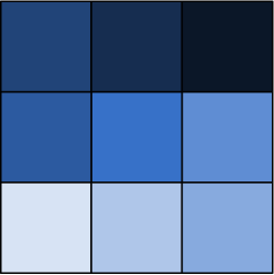
Figure 1: Substructuring

We solve the problem with a BDD solver (primal approach). We use the Flux-free technique [20] to build statically admissible stress fields; each star-patch problem is solved by subdividing each element into 12 elements (h-refinement technique). For the sake of simplicity, we note:

• $\rho=\frac{|L(\underline{w})-a(\underline{u}_{D},\underline{w})|}{\sqrt{\sum_{s}\vvvert\underline{w}^{(s)}\vvvert_{\Omega^{(s)}}^{2}}}$ the lower bound of the error

• $\rho_{discr}=\frac{|L(\underline{w})-a(\underline{u}_{N},\underline{w})|}{\sqrt{\sum_{s}\vvvert\underline{w}^{(s)}\vvvert_{\Omega^{(s)}}^{2}}}$ the discretization part of the lower bound

• $\rho_{alg}=\frac{|a(\underline{u}_{D}-\underline{u}_{N},\underline{w})|}{\sqrt{\sum_{s}\vvvert\underline{w}^{(s)}\vvvert_{\Omega^{(s)}}^{2}}}$ the algebraic part of the lower bound

• $\rho_{bis}=\rho_{discr}-{\alpha}$ the lower bound with separation of sources of error

• $\theta=\sqrt{\sum_{s}{e^{2}_{CR_{\Omega^{(s)}}}(\underline{u}_{D}^{(s)},\hat{\underline{\underline{\sigma}}}_{N}^{(s)})}}$ the upper bound of the error

• $\theta_{discr}=\sqrt{\sum_{s}{e^{2}_{CR_{\Omega^{(s)}}}(\underline{u}_{N}^{(s)},\hat{\underline{\underline{\sigma}}}_{N}^{(s)})}}$ the discretization part of the upper bound

The quantities with the superscript ^seq are computed with a sequential simulation (no substructuring and use of a direct solver).

4.1.1 Effects of the substructuring on the computation of the lower bound at convergence

In this subsection, we compare the lower bound obtained in a sequential simulation with the lower bound obtained in the substructured context when the solver has converged. Since the study is done at convergence, the primal and dual approaches are equivalent.

Figure 2: Evolution of the upper and lower bounds of the error in function of the mesh size h

On figure 2, we observe that the bounds are the same for sequential and substructured computations. We also verify that the exact error is between upper and lower bounds. The convergence is the one expected for such a regular problem (h-slope).

Then, we compare the bounds for several substructuring as illustrated in figure 3. Table 1 gathers the lower bounds for sequential, primal and dual approaches computed at convergence normalized by the bounds for sequential computation. We observe that the substructuring has quasi no influence on the accuracy of the lower bound.

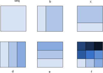
Figure 3: Different substructurings

	seq	b	c	d	e	f
$\frac{\theta}{\theta^{seq}}$	1	1.0002	0.9993	0.9989	1.0004	0.9993
$\frac{\rho}{\rho^{seq}}$	1	0.9981	0.9964	0.9926	0.9958	0.9886

Table 1: Relative upper and lower bounds of the error for various substructuring

4.1.2 Separation of sources of error

In this subsection, we illustrate the separation of sources of error in the lower bound.

On the first graph in figure 4, we give the evolution of the upper and lower bounds and of the true error until the fifth iteration. We observe the fast convergence of those bounds. On the same graph, we also visualize the discretization parts $\theta_{discr}$ and $\rho_{discr}$. The bounding is more precise and enables to define after a few iterations the interval in which the true error is located at convergence. The second graph in figure 4 gives the evolution of the terms in theorem 2. The quantity $\alpha$ scrictly decreases along the iterations, the evolution of the quantity $\rho_{alg}$ is not as smooth.

Figure 4: Separation of sources of error in upper and lower bounds

Figure 5: Evoluation of the two lower bounds during iterations

Figure 5 represents the two lower bounds of theorem 2. As expected, the second lower bound is not precise at the beginning since it gives a negative value. However, the zero of this bound enables to tell the moment when the algebraic error becomes smaller than the discretization error.

4.2 Pre-cracked structure

We now consider a pre-cracked structure decomposed into 16 subdomains as illustrated in Figure 6. The displacements at the base of the structure and on the larger hole are imposed to be zero. The upper-left part and the second hole are subjected to a constant unit pressure. We made the hypothesis of plane stress. The quantity of interest is the mean of the stress component $\sigma_{xx}$ on a region $\omega$ close to the crack. In Figure 6, the loading of the reference problem is in blue and the loading of adjoint problem is in orange. We used the FETI algorithm (dual approach) to solve the interface problem and the statically admissible stress fields are built using the Flux-free technique [3, 20] with h-refinement technique for the solving of local problems on star-patches (each element is divided into 16 elements).

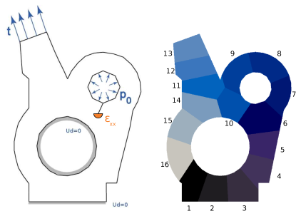
Figure 6: Loading of forward (blue) and adjoint problems (orange), domain decomposition

4.2.1 Separation of sources of error in upper and lower bounds

For this paragraph, we consider only the forward problem. The mesh used for this computation is composed of 4370 degrees of freedom. We compute the global upper and lower bounds during the iterations and the discretization upper and lower bounds along the iterations on the same graph in figure 7.

Figure 7: Pre-cracked structure : Evolution of the upper and lower bounds (global, discretization part, algebraic part) and of the residual during the iterations

As for the previous example, we observe the fast convergence of the upper and lower bounds. This graph also illustrates the separation of sources of error. Finally, we observe that the residual $\alpha$ decreases with the iterations and that, again, the evolution of $\rho_{alg}$ is not as regular.

In figure 8, we give the discretization upper and lower bounds, which define a discretization envelope, for all iterations on the first graph and until the seventh iteration on the second graph.

Figure 8: Pre-cracked structure : Discretization envelope and residual against iterations

The discretization envelope can be used to define the stopping criterion of the solver. In [28], the proposed criterion was to stop when the algebraic error was ten times smaller than the discretization error. On this example, the solver would stop at the sixth iteration. A new stopping criterion could be to stop when the algebraic error is smaller than the discretization part of the lower bound, which would lead to stop to at the fourth iteration.

4.3 Goal-oriented error estimation

In this subsection, we propose an auto-adaptive strategy to steer the iterative solver by an objective of precision on a quantity of interest. In this example, the objective of precision will be five percent. We used the FETI algorithm (dual approach) to solve the interface problem and the statically admissible stress fields are built using the Flux-free technique [20] with h-refinement technique for the solving of local problems on star-patches (each element is divided into 4 elements). Since the forward and adjoint problems are auto-adjoint (due to the symetry of the bilinear form), we solve the two problems simultaneously using a block conjugate gradient (see [27] for more details). The separation of sources of error in the lower bounds of global error on forward and adjoint problem enables the definition of the following criterion : STOP when $\alpha<\rho_{discr}$ and $\widetilde{\alpha}<\widetilde{\rho}_{discr}$ which expresses the fact that the residual is out of the discretization enveloppe so that the algebraic error is negligible in comparaison with the discretization error. Using equation (58), we have the follwing upper and lower bounds on the unknown exact value of the quantity of interest $I_{ex}$:

$$I_{ex}^{-}=I_{H}+\frac{1}{4}\beta^{+}_{inf}-\frac{1}{4}\beta^{-}_{sup}\leq I_{ex}\leq I_{H}+\frac{1}{4}\beta^{+}_{sup}-\frac{1}{4}\beta^{-}_{inf}=I_{ex}^{+}$$ (64)

We will compare the bounds $I_{ex}^{-}$ and $I_{ex}^{+}$ in case the quantities $\beta^{+}_{inf}$ and $\beta^{-}_{inf}$ are computed using expressions in Corollary 1 and in case they are chosen equal to zero ($\beta^{+}_{inf}=\beta^{-}_{inf}=0$), which is equivalent to the bounding in equation (53) with $\underline{u}_{H}=\underline{u}_{D}$, $\underline{\widetilde{u}}_{\widetilde{H}}=\underline{\widetilde{u}}_{D}$, $\hat{\underline{\underline{\sigma}}}_{H}=\hat{\underline{\underline{\sigma}}}_{N}$ and $\hat{\underline{\underline{\widetilde{\sigma}}}}_{\widetilde{H}}=\hat{\underline{\underline{\widetilde{\sigma}}}}_{N}$.

We start with a first mesh which is a little bit refined near the quantity of interest in order to have several elements in the region $\omega$. The discretization error is computed at iteration 1 (which is more relevant than the initilization Iteration 0). The criterion is defined and the solver iterates until the criterion is reached. The error is estimated once again to verify that the discretization error has not changed too much. We give in table 2 the evolution of the residual for forward and adjoint problems and the bounds on the global errors for the two problems.

Iteration	$\theta_{discr}$	$\rho_{discr}$	$\widetilde{\theta}_{discr}$	$\widetilde{\rho}_{discr}$	$\alpha$	$\widetilde{\alpha}$
0					260.07	0.26041
1	11.45	7.0008	0.12867	1.5457 $10^{-3}$	48.339	0.14931
2					35.991	8.5664 $10^{-2}$
3					16.649	4.8205 $10^{-2}$
4					5.5966	1.2462 $10^{-2}$
5					3.5765	8.4996 $10^{-3}$
6	9.9004	6.7105	0.12682	1.5893 $10^{-3}$	0.94805	1.5156 $10^{-3}$

Table 2: Pre-cracked structure: First mesh

Regarding the quantity of interest, at the sixth iteration, we obtain the values presented in table 3.

$I_{H}$	$\beta^{-}_{inf}$	$\beta^{+}_{inf}$	$\frac{1}{4}\beta^{+}_{sup}$	$\frac{1}{4}\beta^{-}_{sup}$
3.1505	1.0087	1.2129	0.68424	0.57132

Table 3: Pre-cracked structure: First mesh : error estimation

In table 4, we give the upper and lower bounds of the unknown exact value $I_{ex}$ of the quantity of interest with and without the use of the lower bounds. We observe that the use of the lower bounds enables to reduce the width by 44 %. At the end of the first solving, the error on the quantity of interest is 22.224 %.

	$I_{ex}^{+}$	$I_{ex}^{-}$	width	precision
With $\beta_{inf}^{+}=\beta_{inf}^{-}=0$	3.8347	2.5791	1.2555	39.852 %
With $\beta_{inf}^{+}$ and $\beta_{inf}^{-}$ from table 3	3.5825	2.8824	0.7001	22.224 %

Table 4: Pre-cracked structure: First mesh : bounds for the exact quantity of interest

We also give, for both problems, the contribution from each subdomain thanks to the following quantities :

$$\eta^{(s)}=\frac{{e_{CR_{\Omega^{(s)}}}(\underline{u}_{N}^{(s)},\hat{\underline{\underline{\sigma}}}_{N}^{(s)})}}{\sqrt{\sum_{s}{e^{2}_{CR_{\Omega^{(s)}}}(\underline{u}_{N}^{(s)},\hat{\underline{\underline{\sigma}}}_{N}^{(s)})}}}\qquad\text{and}\qquad\widetilde{\eta}^{(s)}=\frac{{e_{CR_{\Omega^{(s)}}}(\underline{\widetilde{u}}_{N}^{(s)},\hat{\underline{\underline{\widetilde{\sigma}}}}_{N}^{(s)})}}{\sqrt{\sum_{s}{e^{2}_{CR_{\Omega^{(s)}}}(\underline{\widetilde{u}}_{N}^{(s)},\hat{\underline{\underline{\widetilde{\sigma}}}}_{N}^{(s)})}}}$$ (65)

and plot the contributions on the Figure 9.

Figure 9: First mesh : Distribution of the error estimator within subdomains

As expected, for the adjoint problem, the error is mainly located in the sixth subdomain, which is the subdomain with the load. For the forward problem, the error is more diffuse.

In order to reach the objective of precision, we decide to first improve the quality of the solution of the forward problem. To do so, since the error is not located in few subdomains, we decide to refine the mesh on the whole structure. Of course, we could have used the error map provided by the error estimator and a remeshing criterion to process adaptive remeshing (see for instance [33, 5, 17, 2, 6]). For sake of simplicity, a refinement by splitting is performed. We also reuse the search directions computed during the first solving in order to speed up the next one. The 12 interface vectors (2 interface vectors -one for the forward problem, one for the adjoint problem- computed at each iteration of the first solving that converged in 6 iterations) corresponding to the search directions are projected on the new mesh and used as additional constraints thanks to augmented-Krylov methods [31]. Since the dual approach was chosen, we use a two-level FETI algorithm [8] to take into account the additional constraints. It does not modify the methodology to construct admissible fields nor the error estimator. Recycling search directions leading to a better initilization, we compute the error estimation at iteration 0 and define the stopping criterion. Once the criterion is reached, the error is estimated once again and if the criterion is checked, the solver is stopped. We give in the table 5 the evolution of the residuals and of the bounds on the global errors for the forward and adjoint problems. We can observe that the first residual is comparable to the last residual of the first solving.

Iteration	$\theta_{discr}$	$\rho_{discr}$	$\widetilde{\theta}_{discr}$	$\widetilde{\rho}_{discr}$	$\alpha$	$\widetilde{\alpha}$
0	5.7611	3.8882	7.5633 $10^{-2}$	7.551 $10^{-4}$	5.7017	7.4954 $10^{-3}$
1					3.3265	4.4442 $10^{-3}$
2					1.2869	8.4996 $10^{-4}$
3	5.4304	3.7882	7.5564 $10^{-2}$	7.6332 $10^{-4}$	0.31197	2.4632 $10^{-4}$

Table 5: Pre-cracked structure: Second mesh

Regarding the quantity of interest, we obtain the values presented in table 6.

$I_{H}$	$\beta^{-}_{inf}$	$\beta^{+}_{inf}$	$\frac{1}{4}\beta^{+}_{sup}$	$\frac{1}{4}\beta^{-}_{sup}$
3.2266	0.32673	0.43838	0.23661	0.17372

Table 6: Pre-cracked structure: Second mesh : error estimation

In table 7, we give the upper and lower bounds of the unknown exact value $I_{ex}$ of the quantity of interest with and without the use of the lower bounds. We observe that the use of the lower bounds improves the bounding. At the end of the second solving, the uncertainty on the quantity of interest is 6.7893 %.

	$I_{ex}^{+}$	$I_{ex}^{-}$	width	precision
With $\beta_{inf}^{+}=\beta_{inf}^{-}=0$	3.4632	3.0528	0.41034	12.717 %
With $\beta_{inf}^{+}$ and $\beta_{inf}^{-}$ from table 6	3.3815	3.1624	0.21906	6.7893 %

Table 7: Pre-cracked structure: Second mesh : bounds for the exact quantity of interest

In order to reach the objective of precision, we decide to refine the mesh only for the sixth subdomain to improve the quality of the adjoint solution. Refining this subdomain’s discretization introduces incompatibilities at the interface that can be easily managed thanks to transfer matrix as explained in [27]. This incompatibility does not affect the error estimator since the quantity of interest is located far from the subdomain’s boundary. Once again, we reuse the search directions of the first two solutions to speed up the third solving. As the discretization of the interface is not modified (see [27]), the interface vectors can be directly used as additional constraints.

Iteration	$\theta_{discr}$	$\rho_{discr}$	$\widetilde{\theta}_{discr}$	$\widetilde{\rho}_{discr}$	$\alpha$	$\widetilde{\alpha}$
0	5.1501	3.5841	4.6197 $10^{-2}$	2.9485 $10^{-4}$	0.32764	6.2878 $10^{-4}$
1	5.1267	3.5824	4.619 $10^{-2}$	2.9482 $10^{-4}$	0.10619	1.6588 $10^{-4}$

Table 8: Pre-cracked structure: Third mesh

Regarding the quantity of interest, we obtain the values presented in table 9.

$I_{H}$	$\beta^{-}_{inf}$	$\beta^{+}_{inf}$	$\frac{1}{4}\beta^{+}_{sup}$	$\frac{1}{4}\beta^{-}_{sup}$
3.2625	0.18986	0.25873	0.13618	0.10058

Table 9: Pre-cracked structure: Third mesh : error estimation

In table 10, we give the upper and lower bounds of the unknown exact value $I_{ex}$ of the quantity of interest with and without the use of the lower bounds. We observe that the use of the lower bounds enables to reduce the width by 44 %. At the end of the third solving, the objective of precision is reached and the error on the exact value of the quantity of interest is smaller than 4 %.

	$I_{ex}^{+}$	$I_{ex}^{-}$	width	precision
With $\beta_{inf}^{+}=\beta_{inf}^{-}=0$	3.3986	3.1619	0.2367	7.2574 %
With $\beta_{inf}^{+}$ and $\beta_{inf}^{-}$ from table 9	3.3512	3.2265	0.1247	3.8199%

Table 10: Pre-cracked structure: Third mesh : bounds for the exact quantity of interest

Finally, we give the global errors and residuals against cumulative iteration on Figure 10 and the evolution of the approximated value of the quantity of interest $I_{H}$ and the upper and lower bounds for $I_{ex}$ in Figure 11.

Figure 10: Pre-cracked structure : Discretization envelope and residual against cumulative iterations

Figure 11: Pre-cracked structure : Evolution of the approximated quantity of interest $I_{H}$ and of the bounds of the exact value $I_{ex}$

5 Conclusion

In this paper, we proposed a strict lower bound of the error in a substructured context which can be computed in parallel using the admissible fields built for the computation of the upper bound. Moreover, a theorem gives a second lower bound that separates the algebraic error from the discretization error. As illustrated on mechanical examples, the lower bounds are quasi independent from the substructuring and are as accurate as the sequential lower bound. The examples also show the separation of sources of error for the lower bound. Finally, we proposed an auto-adaptive strategy to steer the iterative solver by an objective of precision on a quantity of interest. Benefiting from the separation of sources of error to avoid oversolving and the recycling of Krylov subspaces, the strategy automatically defines a sequence of optimized solvings.

Acknoledgment

The authour would like to thank Professor Pedro Diez (Universitat Politècnica de Catalunya) for the helpful and fruitful discussions.

References

- [1] R. Becker and R. Rannacher. A feed-back approach to error control in finite element methods: Basic analysis and examples. Journal of Numerical Mathematics, 4:237–264, 1996.
- [2] Emmanuel Bellenger and Patrice Coorevits. Adaptive mesh refinement for the control of cost and quality in finite element analysis. Finite Elements in Analysis and Design, 41(15):1413 – 1440, 2005.
- [3] R. Cottereau, P. Díez, and A. Huerta. Strict error bounds for linear solid mechanics problems using a subdomain-based flux-free method. Computational Mechanics, 44(4):533–547, 2009.
- [4] P. Díez, N. Parés, and A. Huerta. Recovering lower bounds of the error by postprocessing implicit residual a posteriori error estimates. International Journal for Numerical Methods in Engineering, 56(10):1465–1488, 2003.
- [5] Pedro Díez and Antonio Huerta. A unified approach to remeshing strategies for finite element h-adaptivity. Computer Methods in Applied Mechanics and Engineering, 176(1-4):215–229, 1999.
- [6] Pedro Díez, Juan José Ródenas, and Olgierd C. Zienkiewicz. Equilibrated patch recovery error estimates: simple and accurate upper bounds of the error. International Journal for Numerical Methods in Engineering, 69(10):2075–2098, 2007.
- [7] C. Farhat and F. X. Roux. The dual schur complement method with well-posed local neumann problems. Contemporary Mathematics, 157:193–201, 1994.
- [8] Charbel Farhat and Jan Mandel. The two-level FETI method for static and dynamic plate problems part I: An optimal iterative solver for biharmonic systems. Computer Methods in Applied Mechanics and Engineering, 155(1–2):129 – 151, 1998.
- [9] L. Gallimard. A constitutive relation error estimator based on traction-free recovery of the equilibrated stress. International Journal for Numerical Methods in Engineering, 78(4):460–482, 2009.
- [10] P. Gosselet, C. Rey, and J. Pebrel. Total and selective reuse of krylov subspaces for the resolution of sequences of nonlinear structural problems. International Journal for Numerical Methods in Engineering, 94(1):60–83, 2013.
- [11] Pierre Gosselet and Christian Rey. Non-overlapping domain decomposition methods in structural mechanics. Archives of Computational Methods in Engineering, 13(4):515–572, 2006.
- [12] P. Ladevèze. Upper error bounds on calculated outputs of interest for linear and nonlinear structural problems. Comptes Rendus Académie des Sciences - Mécanique, Paris, 334(7):399–407, 2006.
- [13] P. Ladevèze. Strict upper error bounds on computed outputs of interest in computational structural mechanics. Computational Mechanics, 42(2):271–286, 2008.
- [14] P. Ladevèze and D. Leguillon. Error estimate procedure in the finite element method and application. SIAM Journal of Numerical Analysis, 20(3):485–509, 1983.
- [15] P. Ladevèze and J. P. Pelle. Mastering Calculations in Linear and Nonlinear Mechanics. Springer, New York, 2004.
- [16] Patrick Le Tallec. Domain decomposition methods in computational mechanics. Comput. Mech. Adv., 1(2):121–220, 1994.
- [17] J. T. Oden and S. Prudhomme. Goal-oriented error estimation and adaptivity for the finite element method. Computers & Mathematics with Applications, 41(5-6):735–756, 2001.
- [18] S. Ohnimus, E. Stein, and E. Walhorn. Local error estimates of fem for displacements and stresses in linear elasticity by solving local neumann problems. International Journal for Numerical Methods in Engineering, 52(7):727–746, 2001.
- [19] M. Paraschivoiu, J. Peraire, and A. T. Patera. A posteriori finite element bounds for linear-functional outputs of elliptic partial differential equations. Computer Methods in Applied Mechanics and Engineering, 150(1-4):289–312, 1997.
- [20] N. Parés, P. Díez, and A. Huerta. Subdomain-based flux-free a posteriori error estimators. Computer Methods in Applied Mechanics and Engineering, 195(4-6):297–323, 2006.
- [21] N. Parés, H. Santos, and P. Díez. Guaranteed energy error bounds for the poisson equation using a flux-free approach: Solving the local problems in subdomains. International Journal for Numerical Methods in Engineering, 79(10):1203–1244, 2009.
- [22] A. Parret-Fréaud, C. Rey, P. Gosselet, and F. Feyel. Fast estimation of discretization error for fe problems solved by domain decomposition. Computer Methods in Applied Mechanics and Engineering, 199(49-52):3315–3323, 2010.
- [23] F. Pled, L. Chamoin, and P. Ladevèze. On the techniques for constructing admissible stress fields in model verification: Performances on engineering examples. International Journal for Numerical Methods in Engineering, 88(5):409–441, 2011.
- [24] S. Prudhomme and J. T. Oden. On goal-oriented error estimation for elliptic problems: application to the control of pointwise errors. Computer Methods in Applied Mechanics and Engineering, 176(1-4):313–331, 1999.
- [25] Christian Rey and Franck Risler. A rayleigh–ritz preconditioner for the iterative solution to large scale nonlinear problems. Numerical Algorithms, 17(3/4):279–311, 1998.
- [26] V. Rey, P. Gosselet, and C. Rey. Study of the strong prolongation equation for the construction of statically admissible stress fields: Implementation and optimization. Computer Methods in Applied Mechanics and Engineering, 268(0):82 – 104, 2014.
- [27] Valentine Rey, Pierre Gosselet, and Christian Rey. Strict bounding of quantities of interest in computations based on domain decomposition. Computer Methods in Applied Mechanics and Engineering, 287(0):212 – 228, 2015.
- [28] Valentine Rey, Christian Rey, and Pierre Gosselet. A strict error bound with separated contributions of the discretization and of the iterative solver in non-overlapping domain decomposition methods. Computer Methods in Applied Mechanics and Engineering, 270(0):293 – 303, 2014.
- [29] F. Risler and C. Rey. Iterative accelerating algorithms with krylov subspaces for the solution to large-scale non-linear problems. Numerical algorithms, 23:1–30, 2000.
- [30] Y. Saad. Iterative methods for sparse linear systems. Society for Industrial and Applied Mathematics, Philadelphia, 3rd edition edition, 2003.
- [31] Yousef Saad. Analysis of augmented krylov subspace methods. SIAM Journal on Matrix Analysis and Applications, 18(2):435–449, 1997.
- [32] T. Strouboulis, I. Babuška, D. K. Datta, K. Copps, and S. K. Gangaraj. A posteriori estimation and adaptive control of the error in the quantity of interest. part I: A posteriori estimation of the error in the von mises stress and the stress intensity factor. Computer Methods in Applied Mechanics and Engineering, 181(1–3):261–294, 2000.
- [33] R. Verfürth. A Review of A Posteriori Error Estimation and Adaptive Mesh-refinement Techniques. Wiley-Teubner, Stuttgart, 1996.