Cutoff for random walks on graphs with bottlenecks.

Abstract.

We examine the mixing time for random walks on graphs. In particular we are interested on investigating graphs with bottlenecks. Furthermore, the cutoff phenomenon is examined.

1. Introduction.

Assume $X$ is an irreducible aperiodic Markov chain on some finite state space. Consider $P$ to be the transition matrix and $\pi$ the stationary distribution. At first define the total variation distance between two measures $\mu$ and $\nu$ to be

$$||\mu-\nu||=\sup_{A}|\mu(A)-\nu(A)|.$$

Then for every $\epsilon>0$ we define the $\epsilon$-total variation mixing time as

$$t_{mix}(\epsilon)=\min\{t\geq 0:\max_{x}||P^{t}(x,\dot{)}-\pi||\leq\epsilon\}.$$

The purpose of the current paper is to calculate upper and lower bounds for the mixing time of an irreducible Markov chain on graphs with bottlenecks. We aim in extending the example presented by Peres and Sousi in [2] to a general result that will include cases not covered yet. In particular, we are interested in determining conditions under which the upper and lower bounds of the mixing time are asymptotically equal.

Figure 1. Case A.

Furthermore, some outcomes in relation to the cutoff phenomena are obtained.

We say that the sequence of chains $X^{n}$ exhibits total variation cutoff if for every $0<\epsilon<1$

(1.1) $$\lim_{n\rightarrow\infty}\frac{t_{mix}^{n}(\epsilon)}{t_{mix}^{n}(1-\epsilon)}=1.$$

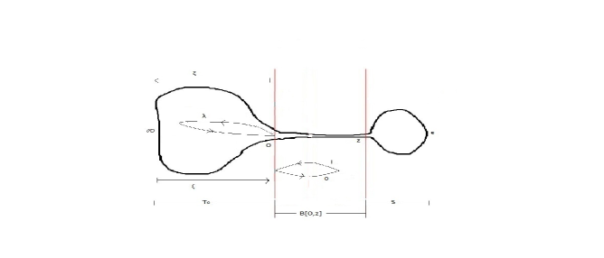
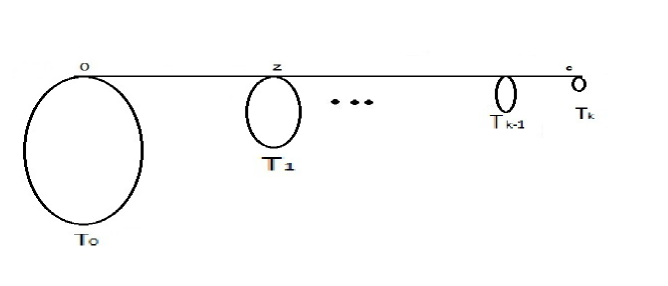
In [2] the first example of a tree was constructed which exhibits total variation cutoff. The construction of the tree was based on placing a binary tree consisting of $N=n_{k}^{3}$ vertices at the origin of a line of $n_{k}$ points, where $n_{k}=2^{2^{k}}$. Then for every $j\in\{[k/2],...,k\}$ a binary tree $T_{j}$ consisting of $N/n_{j}$ vertices was placed at distance $n_{j}$ from the origin. The purpose of the current paper is to generalise this result. We will consider two cases, one general case referred to as Case A (see figure 1) where we will consider two graphs connected with a bottleneck and another one referred to as Case B (see figure 2), where we will substitute the trees $T_{j}$ in [2] by finite graphs $T_{j}$ in such a way that a bottleneck is observed between the $T_{j}$ ’s.

Figure 2. Case B.

We will denote by $B[0,z]$ the bottleneck of the graph, the part of the graph between $0$ and $z$, that is the part of the graph between $T_{0}$ and $S$. All components of the graph, $T_{i},S_{i},B[0,z],S$ increase in size as $k$ increases. We will denote $D=T_{0}\cup B[0,z]$ while the complement of $D$ will be denoted as $S=D^{c}$. Furthermore, we will denote $\partial D$ the points of $T_{0}$ that are further from $0$, i.e. $\partial D:=\left\{x\in T_{0}\text{\ : \ }d(x,0)=\max_{x\in T_{0}}d(x,0)\right\}$, where $d(x,y)$ the graph distance between to points $x,y$ of the graph. In Case A we will denote $c$ the right end point of $S$, while in case B, $c$ will be the connecting point between $T_{k}$ and the rest of the graph. We will consider the size of the bottleneck and $S$ to be relatively small compared with how the size of $T_{0}$ increases, in such a way that

$$(C1)\ \ \ \ \ \ \pi(B[0,z]\cup S)\rightarrow 0\text{ \ as \ }k\rightarrow\infty.$$

We define $q$ to be the probability at every return to $T_{0}$ the random walk to exit $T_{0}$ without hitting $\partial D$. Then, $p=1-q$, is the probability at every return to $T_{0}$, the random walk to hit $\partial D$ of $T_{0}$ before exiting $T_{0}$. For instance, if $T_{0}$ is a binary tree, as is the case examined in [2], $q=1-p\geq\frac{1}{3}$.

By $\tau_{x}$ we define the first time we reach $x$

$$\tau_{x}=inf\{t:x_{t}=x\}.$$

Thus, $\tau_{z}$ denotes the first time we reach the boundary between $S$ and $D$. Furthermore, we define

$$\tau^{*}_{x}=inf\{s\geq\tau_{0}:x_{s}=x\}.$$

Through out this paper we will use the symbol $\prec$ to denote domination, i.e. we will write

$$A\prec B\Leftrightarrow\lim_{k\rightarrow+\infty}\frac{A}{B}=0$$

Furthermore, we will write

$$A\asymp B\Leftrightarrow\ \ni\ \text{constant}\ c\ \text{s.t.}\ A=cB$$

and

$$A\lesssim\ B\Leftrightarrow\ \ni\ \text{constant}\ c\ \text{s.t.}\ A\leq cB.$$

We will now look at the main conditions and results of the paper. We focus on the two distinct conditions (H1) and (H2) that result in the two theorems of the paper. The remaining set of conditions labelled as (H) and (C) is common in the two theorems. The main condition states that for some $\gamma$ and $\delta$ increasing on $k$ the following holds

$$(H1)\ \ \ \ \ \ \mathbb{E}_{c}(\tau_{0})+\frac{\gamma}{2}\sqrt{Var_{c}(\tau_{0})}\geq\mathbb{E}_{\partial D}(\tau_{0})+\delta\ \sqrt{Var_{\partial D}(\tau_{0})}$$

for large $k$, with the growth of $\gamma$ being constrained by

$$(H)(a)\ \ \gamma\sqrt{Var_{c}(\tau_{0})}\prec\mathbb{E}_{c}(\tau_{0}).$$

Then we show that $t_{mix}(\epsilon)\sim\mathbb{E}_{c}(\tau_{0})$. This is the results presented in Theorem 1.1. In this category belongs the example presented in [2], as explained in section 4.1. Then we look on graphs that (H1) does not hold. It appears that with some additional conditions the statement of the theorem derived under (H1) still holds true. Assume that the opposite inequality of (H1) holds, that is:

$$\mathbb{E}_{c}(\tau_{0})+\frac{\gamma}{2}\sqrt{Var_{c}(\tau_{0})}\leq\mathbb{E}_{\partial D}(\tau_{0})+\delta\ \sqrt{Var_{\partial D}(\tau_{0})}$$

for large $k$. We will determine conditions so that an asymptotic estimate of the mixing time can be obtained in this case as well. Denote $t_{S}=\mathbb{E}_{c}(\tau_{0})-\gamma\sqrt{Var_{c}(\tau_{0})}$, and consider some $\epsilon\in(0,1)$. Assume that for $k$ large, $\pi(S)+\sqrt{\Phi}<1-\epsilon$ for $\Phi$ defined as

(1.2) $$\Phi=\sum_{x\in S}\frac{\pi(x)}{\pi(S)}P_{x}(t_{S}>\tau_{0}),$$

a function that decreases to zero as $k\rightarrow\infty$. If in addition $D$ and $S$ are such that the following inequality (H2) holds for large $k$

$$\frac{\mathbb{E}_{c}(\tau_{0})+\frac{\gamma}{2}\sqrt{Var_{c}(\tau_{0})}}{\sqrt{\Phi}}\geq\mathbb{E}_{\partial D}(\tau_{0})+\delta\ \sqrt{Var_{\partial D}(\tau_{0})}\geq\mathbb{E}_{c}(\tau_{0})+\frac{\gamma}{2}\sqrt{Var_{c}(\tau_{0})},$$

then $t_{mix}(\epsilon)\sim\frac{\mathbb{E}_{c}(\tau_{0})}{\sqrt{\Phi}}$. This will be the subject of Theorem 1.3. One should notice that the right inequality of (H2) is nothing else than the inverse of (H1). Furthermore, $\sqrt{\Phi}$ is not a constant but a decreasing function such that $\sqrt{\Phi}\downarrow 0$ as $k\rightarrow\infty$. Specific examples are presented in sections 4.2 and 4.3. In this way we can even consider examples that go far from (H1), such that

$$\frac{\mathbb{E}_{c}(\tau_{0})+\frac{\gamma}{2}\sqrt{Var_{c}(\tau_{0})}}{\mathbb{E}_{\partial D}(\tau_{0})+\delta\ \sqrt{Var_{\partial D}(\tau_{0})}}\rightarrow 0\ \ \ \text{as}\ \ k\rightarrow\infty.$$

For both cases investigated in theorems 1.1 and 1.3 cutoff properties are proven in corollaries 1.2 and 1.4.

Some further assumptions on the graph. In relation to the bottleneck we also define

(1.3) $$L_{z}=\sum_{s=\tau_{0}}^{\tau^{*}_{z}}\mathcal{I}(x_{s-1}\notin T_{0},x_{s}\in T_{0})$$

the number of returns to $T_{0}$ in the time interval $[\tau_{0},\tau^{*}_{z}]$. We also assume that the part of the graph between $0$ and $z$ is such that there exists an increasing function $h$, $\lim_{x\rightarrow\infty}h(x)=\infty$, such that

$$(C2)\ \ \ \ \ \ \ \ \ P(L_{z}\leq z)\leq\frac{1}{h(z)}.$$

For the analogue of the example in [2] where the bottle neck is a line, $h(x)=x$.

We define $(\theta_{i})$ to be iid variables distributed as the length of a random walk on $B[0,z]$ starting from $0$ conditioning not to hit $z$ and $(\lambda_{i,j})$ to be iid random variables distributed as the length of a random walk from $0$ on $T_{0}$ conditioning not to hit $\partial T_{0}$, the edge of $T_{0}$. For $n_{i}$ the point where $T_{i}$ connects with the rest of the graph, we denote for every $i\geq 1$, $\partial T_{i}:=\left\{x\in T_{i}\text{\ : \ }d(x,n_{i})=\max_{x\in T_{i}}d(x,n_{i})\right\}$, that is the points in $T_{i}$ that lie at the biggest distance far from $n_{i}$, and so the rest of the graph $T_{i}^{c}$. We will also assume

$$(C3)\ \ \ \ \ \ \mathbb{E}_{0}(\tau_{\partial D}) \leq\mathbb{E}_{\partial D}(\tau_{0})$$

$$\mathbb{E}_{\partial T_{i}}(n_{i}) \leq\mathbb{E}_{\partial D}(\tau_{0})\ \ \forall i$$

for large $k$. Conditions (C3) are reasonable enough since they roughly state that the time needed to traverse the big set of vertices with the complex structure $T_{0}$ is bigger than the smaller $T_{i}$’s, as well as, that when in $T_{0}$, the random walk moves with bigger probability towards the left end side $\partial D$ than towards the bottleneck. The main theorem about the mixing time follows.

Theorem 1.1.

Assume conditions (C) and that for large $k$ there exist $\gamma$ and $\delta$ such that

$$(H)(a)\ \ \gamma\sqrt{Var_{c}(\tau_{0})}\prec\mathbb{E}_{c}(\tau_{0})\text{ \ and \ }(b)\ \mathbb{E}_{\partial D}(\tau_{0})+\mathbb{E}[L]\mathbb{E}[\lambda_{i,j}+\theta_{i}]\prec\gamma\sqrt{Var_{c}(\tau_{0})}$$

and

$$(H1)\ \ \ \ \ \ \mathbb{E}_{c}(\tau_{0})+\frac{\gamma}{2}\sqrt{Var_{c}(\tau_{0})}\geq\mathbb{E}_{\partial D}(\tau_{0})+\delta\ \sqrt{Var_{\partial D}(\tau_{0})}$$

hold. Then for every $0<\epsilon<1$ the mixing time for the random walk on the graph is

$$t^{k}_{mix}(\epsilon)\sim\mathbb{E}_{c}(\tau_{0})$$

In relation then to the cutoff phenomenon, we obtain the following corollary.

Corollary 1.2.

Under the conditions of Theorem 1.1 the random walk on the graph exhibits variation cutoff, that is for every $0<\epsilon<1$

$$\lim_{k\rightarrow\infty}\frac{t_{mix}^{k}(\epsilon)}{t_{mix}^{k}(1-\epsilon)}=1.$$

For an example that satisfies the conditions of Theorem 1.1 one can look on graphs similar to the one presented in [2] as described in section 4.1.

In the case where condition (H1) is not satisfied then an analogue result still holds as presented on the next theorem. First, recall that because of (C1), $\lim_{k\rightarrow\infty}\pi(S)=0$.

Theorem 1.3.

Assume that $\Phi=\sum_{x\in S}\frac{\pi(x)}{\pi(S)}P_{x}(t_{S}>\tau_{0})\downarrow 0$ as $k\rightarrow\infty$. For $\epsilon\in(0,1)$, assume $k$ large enough so that $\pi(S)+\sqrt{\Phi}<1-\epsilon$. Assume conditions (C) and that for large $k$ there exist $\gamma$ and $\delta$ such that

$$(H)\ (a)\ \ \gamma\sqrt{Var_{c}(\tau_{0})}\prec\mathbb{E}_{c}(\tau_{0})\text{ \ and \ }(b)\ \mathbb{E}_{\partial D}(\tau_{0})+\mathbb{E}[L]\mathbb{E}[\lambda_{i,j}+\theta_{i}])\prec\frac{\gamma\sqrt{Var_{c}(\tau_{0})}}{\sqrt{\Phi}}$$

and

$$(H2)\ \ \ \ \ \ \frac{\mathbb{E}_{c}(\tau_{0})+\frac{\gamma}{2}\sqrt{Var_{c}(\tau_{0})}}{\sqrt{\Phi}}\geq\mathbb{E}_{\partial D}(\tau_{0})+\delta\ \sqrt{Var_{\partial D}(\tau_{0})}\geq\mathbb{E}_{c}(\tau_{0})+\frac{\gamma}{2}\sqrt{Var_{c}(\tau_{0})}.$$

Then,

$$t^{k}_{mix}(\epsilon)\sim\frac{\mathbb{E}_{c}(\tau_{0})}{\sqrt{\Phi}}.$$

In sections 4.2 and 4.3 two examples that satisfy the conditions of Theorem 1.3 are presented. As an outcome of the theorem, we obtain the following corollary about variation cutoff.

Corollary 1.4.

Under the conditions of Theorem 1.3 the random walk $X^{n}$ exhibits variation cutoff, that is, for every $0<\epsilon<1$

$$\lim_{k\rightarrow\infty}\frac{t_{mix}^{k}(\epsilon)}{t_{mix}^{k}(1-\epsilon)}=1.$$

From Theorem 1.3 we can obtain the following weaker version, which will be used to show the examples of section 4.

Theorem 1.5.

Assume that $\Phi=\sum_{x\in S}\frac{\pi(x)}{\pi(S)}P_{x}(t_{S}>\tau_{0})\downarrow 0$ as $k\rightarrow\infty$. For $\epsilon\in(0,1)$, assume $k$ large enough so that $\pi(S)+\sqrt{\Phi}<1-\epsilon$. Assume conditions (C) and that for large $k$ there exist $\gamma$ and $\delta$ such that (H) and

$$\mathbb{E}_{\partial D}(\tau_{0})\prec\delta\ \sqrt{Var_{\partial D}(\tau_{0})}$$

and that for $k$ large

$$\mathbb{E}_{c}(\tau_{0})\leq\delta\ \sqrt{Var_{\partial D}(\tau_{0})}\leq\frac{\mathbb{E}_{c}(\tau_{0})}{\sqrt{\Phi}}.$$

Then

$$t_{mix}(\epsilon)\sim\frac{\mathbb{E}_{c}(\tau_{0})}{\sqrt{\Phi}}.$$

A few words about the proof of the two theorems and the structure of the paper. In order to find the asymptotic limits of the mixing time $t^{k}_{mix}$ we will calculate upper and lower bounds for $t^{k}_{mix}(\epsilon)$. Under the conditions of Theorem 1.1, for $0<\epsilon<1$ we will show that for large $k$

(1.4) $$\mathbb{E}_{c}(\tau_{0})-\gamma\sqrt{Var_{c}(\tau_{0})}\leq t^{k}_{mix}(\epsilon)\leq\mathbb{E}_{c}(\tau_{0})+\gamma\sqrt{Var_{c}(\tau_{0})}.$$

Then the mixing time and the cutoff property follow because of (H)(a).

Under the conditions of Theorem 1.3, we will show that for $k$ large enough so that $\pi(S)+\sqrt{\Phi}\leq 1-\epsilon$

(1.5) $$\frac{\mathbb{E}_{c}(\tau_{0})-\gamma\sqrt{Var_{c}(\tau_{0})}}{\sqrt{\Phi}}\leq t^{k}_{mix}(\epsilon)\leq\frac{\mathbb{E}_{c}(\tau_{0})+\gamma\sqrt{Var_{c}(\tau_{0})}}{\sqrt{\Phi}}$$

when $k$ is large. Then the mixing time and the cutoff property follow again because of (H)(a).

The lower bound of both (1.4) and (1.5) will be shown in Lemma 2.1 and Proposition 2.2 of section 2 respectively. The upper bound of (1.4) and (1.5) follows from Proposition 3.2 for $A=1$ and $A=\sqrt{\Phi}<1$ respectively.

2. Lower bounds.

In this section we present two lower bounds for the mixing time $t^{k}_{mix}$. The first lower bound is presented in Lemma 2.1. Then under the condition $\Phi=\sum_{x\in S}\frac{\pi(x)}{\pi(S)}P_{x}(t_{S}>\tau_{0})<1$ for large $k$, we prove in Proposition 2.2 a sharper lower bound. The first lower bound for the mixing time follows.

Lemma 2.1.

Assume (C) and $\gamma\rightarrow\infty$ as $k\rightarrow\infty$. The following lower bound for the mixing time holds:

$$t_{mix}(\epsilon)\geq\mathbb{E}_{c}(\tau_{0})-\gamma\sqrt{Var_{c}(\tau_{0})}$$

for large $k$.

The proof of Lemma 2.1 is presented in [2] (lower bound of Theorem 1.1 [2]). We will use this bound in order to show a sharper lower bound on the following proposition.

Denote $\pi_{S}$ the restriction of $\pi$ to $S$, $\pi_{S}(A)=\pi(S\cap A)$ and $\mu_{S}(A)=\frac{\pi_{S}(A)}{\pi(S)}$. In order to prove the second sharper lower bound we will use the approach of [1] for graphs with one bottleneck. The main result related to the lower bound of the mixing time follows in the next proposition.

Proposition 2.2.

For $\epsilon\in(0,1)$, assume $k$ large enough so that $\sqrt{\Phi}+\pi(S)<1-\epsilon$. Then for $k$ large

$$t^{k}_{mix}(\epsilon)\geq\frac{\mathbb{E}_{c}(\tau_{0})-\gamma\sqrt{Var_{c}(\tau_{0})}}{\sqrt{\Phi}}.$$

Proof.

Since from Lemma 2.1 we know that for $k$ large $t^{k}_{mix}\geq\mathbb{E}_{c}(\tau_{0})-\gamma\sqrt{Var_{c}(\tau_{0})}=t_{S}$, there exists an $m\geq 1$ such that $t^{k}_{mix(\epsilon)}=mt_{S}$. In order to bound the total variation distance $\parallel\mu_{S}P^{mt_{S}}-\mu_{S}\parallel_{TV}$ we can use the following bound

$$\parallel\mu_{S}P^{t}-\mu_{S}\parallel_{TV}\leq t\Phi(S),\ \ \ t\in\mathbb{N}$$

where $\Phi(S)=\sum_{x\in S}\sum_{y\notin S}\mu_{S}(x)P(x,y),$ (see (7.14)-(7.15) from [1]). We then obtain

(2.1) $$\parallel\mu_{S}P^{t^{k}_{mix}}-\mu_{S}\parallel_{TV}\leq t^{k}_{mix}\Phi(S)=mt_{S}\Phi(S)=m\Phi\$$

where we have denoted $\Phi=t_{S}\Phi(S)$. We have

$$\parallel\mu_{S}-\pi\parallel_{TV}=\max_{A\subset\Omega}\left|\mu_{S}(A)-\pi(A)\right|\geq\left|\mu_{S}(S^{c})-\pi(S^{c})\right|=\pi(S^{c})$$

since $\mu_{S}(S^{c})=0$. So, using the triangular inequality, we can write

$$1-\pi(S)\leq\parallel\mu_{S}-\pi\parallel_{TV}\leq\parallel\mu_{S}P^{t^{k}_{mix}}-\mu_{S}\parallel_{TV}+\parallel\mu_{S}P^{t^{k}_{mix}}-\pi\ \parallel_{TV}$$

which leads to

$$1-\pi(S)\leq\parallel\mu_{S}P^{t_{mix}}-\mu_{S}\parallel_{TV}+\epsilon$$

If we bound the first term on the right hand by (2.1) we then have

(2.2) $$1-\pi(S)\leq m\Phi+\epsilon$$

which after substituting $m=\frac{t^{k}_{mix(\epsilon)}}{t_{S}}$ gives the following lower bound for $t^{k}_{mix(\epsilon)}$

$$t^{k}_{mix(\epsilon)}\geq\frac{t_{S}}{\frac{\Phi}{1-\pi(S)-\epsilon}}.$$

If we choose $k$ large enough so that

$$\sqrt{\Phi}+\pi(S)+\epsilon\leq 1\ \Rightarrow\ \frac{\Phi}{1-\pi(S)-\epsilon}\leq\sqrt{\Phi}$$

we then obtain the desired lower bound

$$t^{k}_{mix(\epsilon)}\geq\frac{t_{S}}{\sqrt{\Phi}}.$$

∎

3. Upper bound for the cutoff case.

In this section we calculate the upper bound for the mixing time. Technics from [2] will be closely followed. We start with a technical lemma.

Lemma 3.1.

Assume (C2) and $\pi(S)+\sqrt{\Phi}<1-\epsilon$ for large $k$. Denote $t^{\prime}=\frac{\mathbb{E}_{c}(\tau_{0})+\frac{\gamma}{2}\sqrt{Var_{c}(\tau_{0})}}{\sqrt{\Phi}}$, and define the set $B=\{\tau_{0}<t^{\prime}\}$. If

$$(\star)\ \ \ \ \ t^{\prime}\geq\mathbb{E}_{\partial D}(\tau_{0})+\delta\sqrt{Var_{\partial D}(\tau_{0})}$$

then

(3.1) $$P_{x}(B^{c})\leq\frac{16}{\gamma^{2}}+\frac{1}{\delta^{2}}+\frac{4\mathbb{E}_{\partial D}(\tau_{0})}{\frac{\gamma\sqrt{Var_{c}(\tau_{0})}}{\sqrt{\Phi}}}.$$

Proof.

We will first consider $x\in S\cup B[0,z]$. To show (3.1) we will distinguish on the two different cases of graphs denoted as Case A and B, shown on figures 1 and 2 respectively.

For the Case A we have

$$P_{x}(B^{c})= P_{x}(\tau_{0}\geq t^{\prime})\leq P_{c}(\tau_{0}\geq t^{\prime})=P_{c}(\tau_{0}\geq\frac{\mathbb{E}_{c}(\tau_{0})+\frac{\gamma}{2}\sqrt{Var_{c}(\tau_{0})}}{\sqrt{\Phi}})$$

(3.2) $$\leq P_{c}(\tau_{0}\geq\mathbb{E}_{c}(\tau_{0})+\frac{\gamma}{2}\sqrt{Var_{c}(\tau_{0})})\leq\frac{4}{\gamma^{2}}$$

where above we used first that for $k$ large $\sqrt{\Phi}\leq 1$ and then Chebyshev’s inequality.

We will show the same for every $x\in S\cup B[0,z]$ for graphs in Case B. Define $\tau_{1}$ the time it gets to hit $[0,c]$ and $\tau_{2}$ the time it takes to hit $0$ starting from $X_{\tau_{1}}$. Then

$$P_{x}(B^{c})= P_{x}(\tau_{0}\geq t^{\prime})=P_{x}(\tau_{0}\geq\frac{\mathbb{E}_{c}(\tau_{0})+\frac{\gamma}{2}\sqrt{Var_{c}(\tau_{0})}}{\sqrt{\Phi}})\leq$$

(3.3) $$\leq P_{x}(\tau_{1}\geq\frac{\gamma}{4}\frac{\sqrt{Var_{c}(\tau_{0})}}{\sqrt{\Phi}})+P_{x}(\tau_{2}\geq\frac{\mathbb{E}_{c}(\tau_{0})+\frac{\gamma}{4}\sqrt{Var_{c}(\tau_{0})}}{\sqrt{\Phi}})$$

For the first term on the right hand side of (3) we can use Markov inequality to get

$$P_{x}(\tau_{1}\geq\frac{\gamma}{4}\frac{\sqrt{Var_{c}(\tau_{0})}}{\sqrt{\Phi}})\leq\frac{4\mathbb{E}_{x}(\tau_{1})}{\frac{\gamma\sqrt{Var_{c}(\tau_{0})}}{\sqrt{\Phi}}}$$

But for any $x\in T_{i}$

$$\mathbb{E}_{x}(\tau_{1})\leq\mathbb{E}_{\partial T_{i}}(n_{i})\leq\mathbb{E}_{\partial D}(\tau_{0})$$

because of (C3). This leads to

(3.4) $$P_{x}(\tau_{1}\geq\frac{\gamma}{4}\frac{\sqrt{Var_{c}(\tau_{0})}}{A})\leq\frac{4\mathbb{E}_{\partial D}(\tau_{0})}{\frac{\gamma\sqrt{Var_{c}(\tau_{0})}}{\sqrt{\Phi}}}$$

For the second term on the right hand side of (3) we have

$$P_{x}(\tau_{2}\geq\frac{\mathbb{E}_{c}(\tau_{0})+\frac{\gamma}{4}\sqrt{Var_{c}(\tau_{0})}}{\sqrt{\Phi}})\leq P_{x}(\tau_{2}\geq\mathbb{E}_{c}(\tau_{0})+\frac{\gamma}{4}\sqrt{Var_{c}(\tau_{0})})$$

(3.5) $$\leq P_{c}(\tau_{0}\geq\mathbb{E}_{c}(\tau_{0})+\frac{\gamma}{4}\sqrt{Var_{c}(\tau_{0})})\leq\frac{16}{\gamma^{2}}$$

above we used that $\sqrt{\Phi}<1$ for large $k$ and applied Chebyshev’´s inequality. Finally, putting (3.4) and (3) in (3) gives that for every $x\in S\cup B[0,z]$

(3.6) $$P_{x}(B^{c})\leq \frac{16}{\gamma^{2}}+\frac{4\mathbb{E}_{\partial D}(\tau_{0})}{\frac{\gamma\sqrt{Var_{c}(\tau_{0})}}{\sqrt{\Phi}}}$$

for graphs as in Case B. From (3) and (3.6) we obtain that in both Cases A and B, for every $x\in S\cup B[0,z]$ one has

(3.7) $$P_{x}(B^{c})\leq \frac{16}{\gamma^{2}}+\frac{4\mathbb{E}_{\partial D}(\tau_{0})}{\frac{\gamma\sqrt{Var_{c}(\tau_{0})}}{\sqrt{\Phi}}}$$

For both Cases A and B, when $x\in T_{0}$ we have

$$P_{x}(B^{c})=P_{x}(\tau_{0}\geq t^{\prime})\leq P_{\partial D}(\tau_{0}\geq t^{\prime})$$

For $k$ large so that ($\star$) holds, we can bound

(3.8) $$P_{x}(B^{c})\leq P_{\partial D}(\tau_{0}\geq\mathbb{E}_{\partial D}(\tau_{0})+\delta\ \sqrt{Var_{\partial D}(\tau_{0})})\leq\frac{1}{\delta^{2}}$$

where above we used Chebyshev’s inequality. From (3.7) and (3.8) we obtain (3.1) for every $x\in D\cup S$. ∎

The main result about the upper bound of the mixing time follows.

Proposition 3.2.

Assume (C) and that for large $k$ (H) and

$$(\star)\ \ \ \ \ \frac{\mathbb{E}_{c}(\tau_{0})+\frac{\gamma}{2}\sqrt{Var_{c}(\tau_{0})}}{A}\geq\mathbb{E}_{\partial D}(\tau_{0})+\delta\sqrt{Var_{\partial D}(\tau_{0})}$$

for some $A\leq 1$. Then

$$t^{k}_{mix}\leq\frac{\mathbb{E}_{c}(\tau_{0})+\gamma\sqrt{Var_{c}(\tau_{0})}}{A}$$

Proof.

Denote $t=\frac{\mathbb{E}_{c}(\tau_{0})+\gamma\sqrt{Var_{c}(\tau_{0})}}{A}$. We will consider the following coupling. Assume $X_{0}=x$ and $Y_{0}\sim\pi$. We let $X$ and $Y$ move independently until the first time $X$ hits $0$. Then they still continue both moving independently until the moment they collide or reach the same level at $T_{0}$. In this case the coupling changes to the following. $X$ keeps moving as an aperiodic random walk while $Y$ moves closer or further from $0$ if $X$ moves closer or further respectively. Define $\tau$ to be the coupling time.

Then define $E$ to be the event that after hitting $0$ for the first time it reaches $\partial D$ of $T_{0}$ before hitting $z$, i.e.

$$E=\{\tau^{*}_{\partial D}<\tau^{*}_{z}\}$$

as well as the the events

$$A_{L_{z}}=\{L_{z}>z\}.$$

If we define

$$S=inf\{s\geq\tau^{*}_{\partial D}:x_{s}=0\}$$

then on the event $E$, the quantity $S-\tau_{0}$ is dominated by

$$\sum_{i=1}^{L_{z}}\theta_{i}+\sum_{i=1}^{L_{z}}\sum_{j=1}^{G_{i}}\lambda_{i,j}+\zeta+\xi$$

(see [2]) where we recall $(\theta_{i})_{i}$ are iid variables distributed as the length of a random walk on $B[0,z]$ starting from $0$ conditioning not to hit $z$ and $(\lambda_{i,j})$ are iid random variables distributed as the length of a random walk from $0$ on $T_{0}$ conditioning not to hit $\partial T_{0}$. $(G_{i})_{i}$ is a random variable with probability of success $\frac{\{\#j:j\sim 0,j\in B[0,z]\}}{\{\#j:j\sim 0\}}$ and $\xi$ is a random variable distributed as the commute time between $\partial T_{0}$ and $0$. If we use Wald’s identity we obtain

(3.9) $$\mathbb{E}[(S-\tau_{0})\mathcal{I}_{E}]\leq \mathbb{E}[L_{z}]\mathbb{E}[\theta_{i}]+\mathbb{E}[L_{z}]\mathbb{E}[G_{i}]\mathbb{E}[\lambda_{i,j}]+\mathbb{E}[\zeta]+\mathbb{E}[\xi]\lesssim$$

$$\lesssim \mathbb{E}_{\partial D}(\tau_{0})+\mathbb{E}[L_{z}]\mathbb{E}[\lambda_{i,j}]+\mathbb{E}[L_{z}]\mathbb{E}[\theta_{i}]$$

where above we used (C3) for $\mathbb{E}[\xi]=\mathbb{E}_{\partial D}(\tau_{0})$ and $\mathbb{E}[\zeta]=\mathbb{E}_{0}(\tau_{\partial D})$.

We compute

$$P(\tau>t)\leq P(\tau>t,A_{L})+\frac{1}{h(z)}\leq P(\tau>t,A_{L_{z}},E)+\frac{1}{h(z)}+p^{z}$$

where in the first inequality we used (C2) and in the second that $P(E^{c}\mid L_{z})\leq p^{L_{z}}$. Then we obtain

$$P(\tau>t) \leq P(\tau>t,A_{L_{z}},E)+\frac{1}{h(z)}+p^{z}$$

If we use Lemma 3.1 the last one can be bounded by

(3.10) $$P(\tau>t) \leq P(\tau>t,A_{L_{z}},E,B)+\frac{16}{\gamma^{2}}+\frac{1}{\delta^{2}}+\frac{4\mathbb{E}_{\partial D}(\tau_{0})}{\frac{\gamma\sqrt{Var_{c}(\tau_{0})}}{A}}+\frac{1}{h(z)}+p^{z}$$

Now define $F=\{S-\tau_{0}>\frac{\frac{\gamma}{2}\sqrt{Var_{c}(\tau_{0})}}{A}\}$ and $M=\{Y_{\tau_{0}}\in D\}$. Then $P(M^{c})=o(1)$ as $k\rightarrow\infty$ since at time $\tau_{0}$ the random walk $Y$ is stationary, and so, because of (C1) we have that the stationary probability of $T_{0}$ is $1-o(1)$. We observe that on the events $E$ and $M$ the two walks $X$ and $Y$ must have coalesced by time $S$. Therefore

$$B\cap F^{c}\subset\{\tau<t\}$$

This implies that

$$P(\tau>t,A_{L_{z}},E,B) \leq P(\tau>t,A_{L_{z}},E,M,B)+o(1)=P(\tau>t,A_{L_{z}},E,M,B,F)+o(1)\leq$$

$$\leq P(E,F)+o(1)=P(E,\{S-\tau_{0}>\frac{\frac{\gamma}{2}\sqrt{Var_{c}(\tau_{0})}}{A}\})+o(1)$$

From Markov inequality

$$P(\tau>t,A_{L_{z}},E,B)\leq\frac{2\mathbb{E}[(S-\tau_{0})\mathcal{I}_{E}]}{\frac{\gamma\sqrt{Var_{c}(\tau_{0})}}{A}}+o(1)$$

If we now use (3.9) we obtain

(3.11) $$P(\tau>t,A_{L_{z}},E,B)\leq 2\frac{\mathbb{E}_{\partial D}(\tau_{0})+\mathbb{E}[L_{z}]\mathbb{E}[\lambda_{i,j}]+\mathbb{E}[L_{z}]\mathbb{E}[\theta_{i}]}{\frac{\gamma\sqrt{Var_{c}(\tau_{0})}}{A}}+o(1)$$

Combining together (3.10) and (3.11) we get

$$P(\tau>t)\leq 2\frac{\mathbb{E}_{\partial D}(\tau_{0})+\mathbb{E}[L_{z}]\mathbb{E}[\lambda_{i,j}]+\mathbb{E}[L_{z}]\mathbb{E}[\theta_{i}]}{\frac{\gamma\sqrt{Var_{c}(\tau_{0})}}{A}}+\frac{16}{\gamma^{2}}+\frac{1}{\delta^{2}}+\frac{4\mathbb{E}_{\partial D}(\tau_{0})}{\frac{\gamma\sqrt{Var_{c}(\tau_{0})}}{A}}+$$

$$+\frac{1}{h(z)}+p^{z}+o(1)$$

If one takes under account that

$$\max_{x}||P^{t}(x,\dot{)}-\pi||\leq P(\tau>t)$$

(see [1]) we eventually obtain

$$\max_{x}||P^{t}(x,\dot{)}-\pi||\leq 2\frac{\mathbb{E}_{\partial D}(\tau_{0})+\mathbb{E}[L_{z}]\mathbb{E}[\lambda_{i,j}]+\mathbb{E}[L_{z}]\mathbb{E}[\theta_{i}]}{\frac{\gamma\sqrt{Var_{c}(\tau_{0})}}{A}}+\frac{16}{\gamma^{2}}+\frac{1}{\delta^{2}}+\frac{4\mathbb{E}_{\partial D}(\tau_{0})}{\frac{\gamma\sqrt{Var_{c}(\tau_{0})}}{A}}+$$

$$+\frac{1}{h(z)}+p^{z}+o(1)$$

Because of (H)(b), the fact that $h(z),z\rightarrow\infty$ as $k\rightarrow\infty$ (recall $p<1$) and that $A<1$ for large $k$, we obtain $t_{mix}\leq\frac{\mathbb{E}_{c}(\tau_{0})+\gamma\sqrt{Var_{c}(\tau_{0})}}{A}$. ∎

4. Paradigms

In this section we present examples for the two main theorems. At first in paradigm 1 an example that satisfies the conditions of Theorem 1.1 is presented. Then in sections 4.2 and 4.3, two examples that satisfy the conditions of Theorem 1.3 are presented. From these last two, at the first one, paradigm 2, we consider a graph with

$$\mathbb{E}_{\partial D}(\tau_{0})\leq\sqrt{Var_{\partial D}(\tau_{0})}$$

while at the second one, paradigm 3, a graph with

$$\mathbb{E}_{\partial D}(\tau_{0})>\sqrt{Var_{\partial D}(\tau_{0})}.$$

For both examples we establish $\sqrt{\Phi}^{-1}\rightarrow\infty$ as $k\rightarrow\infty$.

4.1. Paradigm 1

This is the example presented in [2].

We will show that condition (H1) is satisfied. Since in the graph presented one has

$$\sqrt{Var_{\partial D}(\tau_{0})}\lesssim\ \mathbb{E}_{\partial D}(\tau_{0})\text{ \ and \ }\sqrt{Var_{c}(\tau_{0})}\lesssim\ \mathbb{E}_{c}(\tau_{0})$$

(see [2]) it is sufficient to show that

(4.1) $$\mathbb{E}_{\partial D}(\tau_{0})\lesssim\sqrt{Var_{c}(\tau_{0})}.$$

Since $N$ is the size of binary tree $T_{0}$, one has that $N=\sum_{j=0}^{l}2^{j}$, were $l$ is the number of levels of $T_{0}$, i.e. $l=\log(N-1)-1$. Concerning (4.1), one can think of the random walk from the leafs $\partial T_{0}$ of the binary tree to the origin $0$ as a walk from $0$ to $l$ on $[0,l]\cap\mathbb{Z}$, with a reflective boundary at $0$ and probabilities $\frac{2}{3}$ and $\frac{1}{3}$ towards the left and the right respectively at any other point of the line. Since, for this one dimensional random walk the hitting time satisfies

$$l^{2}\lesssim\mathbb{E}_{0}(\tau_{l})\lesssim l^{3}$$

we obtain for $T_{0}$ that

(4.2) $$l^{2}\asymp(\log(N-1)-1)^{2}\lesssim\mathbb{E}_{\partial D}(\tau_{0})\lesssim(\log(N-1)-1)^{3}\asymp l^{3}.$$

On the other hand we know that (see [2])

(4.3) $$\sqrt{Var_{c}(\tau_{0})}\asymp N\sqrt{k}.$$

From (4.2) and (4.3) inequality (4.1) follows for appropriately large $N=n_{k}^{3}$ so that

$$(\log(N-1)-1)^{3}\lesssim N\sqrt{k}$$

or if we substitute $N=n_{k}^{3}$

$$n_{k}^{3}<e^{n_{k}k^{\frac{1}{6}}+1}$$

which is true for $n_{k}$ sufficiently large. The rest of the conditions are easily verified directly from [2].

4.2. Paradigm 2

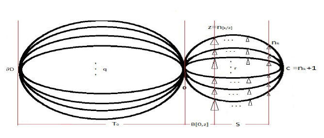
We will construct a graph based partly on the graph $\mathcal{T}$ presented in [2]. Let $n_{k}=2^{2^{k}}$ and consider the line $[0,n_{k}+1]$. Then for all $j\in\{[\frac{k}{2}],...,k\}$ place a binary tree at distance $n_{j}$ from the origin consisting of $\frac{N}{n_{j}}$ vertices. We denote this construction as $G_{0}$. In this way, the part of $G_{0}$ contained between $[0,n_{k}]$, i.e. $G_{0}\smallsetminus\{n_{k}+1\}$, is equal with $\mathcal{T}\smallsetminus T_{0}$ from [2], where $T_{0}$ is the big binary tree at $0$ of $\mathcal{T}$. Then consider $r$ identical copies of $G_{0}$ and glue them together at $0$ and $n_{k}+1$ as shown on figure 3. We also consider $q$ copies of a line $[-m,0]$ and connect them with the previous construction at $0$ and together at $-m$. In this way, we can consider $T_{0}$ to be the part of graph between $[-m,0]$ with $\partial T_{0}=-m$, the bottleneck $B[0,z]$ to be the part of the graph between $0$ and $n_{[\frac{k}{2}]}$, while $S$ is the part between $n_{[\frac{k}{2}]}$ and $n_{k}+1$. In this way $c=n_{k}+1$ and $z=n_{[\frac{n_{k}}{2}]}$.

Figure 3. Paradigm 2

We will determine $m,r,q,\gamma,\delta$ so that the conditions of Theorem 1.5 hold. But first, we will place conditions on the graph so that condition (H1) of Theorem 1.1 is not true. If $X$ is a simple random walk on the interval $[-m,0]$ staring from $-m$, then the mean and the variance of the time it gets to reach $0$ from $m$ for the first time are $\mathbb{E}_{-m}(\tau_{0})=m^{2}$ and $Var_{-m}(\tau_{0})=m^{4}$ respectively. Since $D$ consists of $q$ lines $[-m,0]$ connected on $0$ and $-m$, and when at $-m$ we move at any of the $q$ branches $[-m,0]$ with the same probability $\frac{1}{q}$ we obtain that

$$\mathbb{E}_{\partial D}(\tau_{0})=m^{2}\text{\ \ \ \ and \ \ \ \ }Var_{\partial D}(\tau_{0})=m^{4}.$$

From [2] we know that

$$\sqrt{Var_{c}(\tau_{0})}\asymp N\sqrt{k}\text{ \ \ \ \ \ and \ \ \ \ \ }\mathbb{E}_{c}(\tau_{0})=6Nk+o(N\sqrt{k})\asymp 6Nk.$$

If one chooses

(4.4) $$m^{2}=6Nk$$

then (H1) is not true since $\delta\sqrt{Var_{\partial D}(\tau_{0})}>\mathbb{E}_{c}(\tau_{0})$ for any $\delta=k^{t}$ with $t>0$, and $k$ large. We also notice that for any $\delta=k^{t}$ with $t>0$

$$\mathbb{E}_{\partial D}(\tau_{0})\prec\delta\sqrt{Var_{\partial D}(\tau_{0})}.$$

Furthermore, for any $\gamma=k^{p}$ with $p<\frac{1}{2}$ we get

(4.5) $$\gamma\sqrt{Var_{c}(\tau_{0})}\prec\mathbb{E}_{c}(\tau_{0}).$$

In addition, from (4.5) we get that

(4.6) $$t_{S}=\mathbb{E}_{c}(\tau_{0})-\gamma\sqrt{Var_{c}(\tau_{0})}\prec 6Nk.$$

At first we will show that for appropriate $r>0$ one can obtain $\sqrt{\Phi}<\frac{1}{k^{s}}$ for some $s>0$.

Thus, it suffices to show that $\Phi=t_{S}\sum_{x\in S}\sum_{y\notin S}\mu_{S}(x)P(x,y)<\frac{1}{k^{2s}}$. For that, we compute

(4.7) $$\sum_{x\in S}\sum_{y\notin S}\mu_{S}(x)P(x,y)=\frac{q}{(q+r)\left|S\right|}$$

where the size of $S$ is

(4.8) $$\left|S\right|=r(n_{k}+1+N(\sum_{j\in\{[k/2],...,k\}}\frac{1}{n_{j}}))\asymp rN(\sum_{j\in\{[k/2],...,k\}}\frac{1}{n_{j}}).$$

Combining together (4.6), (4.7) and (4.8) we get

$$\Phi\asymp\frac{6Nkq(\sum_{j\in\{[k/2],...,k\}}\frac{1}{n_{j}})^{-1}}{(q+r)rN}.$$

So, if we choose

(4.9) $$r=12k^{2s+1}(\sum_{j\in\{[k/2],...,k\}}\frac{1}{n_{j}})^{-1}$$

we obtain $\sqrt{\Phi}\downarrow 0$ as $k\rightarrow\infty$. We will now determine parameters so that conditions (C) are satisfied. For (C1) we compute

$$\pi(B[0,z]\cup S)=\frac{\left|S\right|+\left|B[0,z]\right|}{\left|S\right|+\left|B[0,z]\right|+\left|T_{0}\right|}.$$

For this to vanish as $k\rightarrow\infty$ we need

(4.10) $$\left|S\right|+\left|B[0,z]\right|\prec\left|T_{0}\right|.$$

But $\left|S\right|+\left|B[0,z]\right|\asymp rN(\sum_{j\in\{[k/2],...,k\}}\frac{1}{n_{j}})$ and $\left|T_{0}\right|\asymp q(m-2)$. For (C1) to hold true we need $q$ large enough so that

$$\frac{rN}{m-2}(\sum_{j\in\{[k/2],...,k\}}\frac{1}{n_{j}})\prec\ q.$$

If we replace $r$ by (4.9) and $m$ by (4.4) we derive

(4.11) $$\frac{12k^{2s+1}N}{\sqrt{6Nk}-2}\prec\ q.$$

For the condition (C2), we recall that $L_{n_{[k/2]}}=\sum_{s=\tau_{0}}^{\tau^{*}_{n_{[k/2]}}}\mathcal{I}(x_{s-1}\notin T_{0},x_{s}\in T_{0})$. Then, since we move to every branch of the bottleneck with the same probability and the $r$ branches $[0,n_{[k/2]}]$ are identical, $L$ has the geometric distribution with parameter $\frac{1}{n_{[k/2]}}$. This leads to

$$(C2)\ \ \ \ \ \ \ \ \ P(L_{n_{[k/2]}}\leq n_{[k/2]})\leq\frac{1}{n_{[k/2]}}.$$

Concerning (C3), the first assertion $\mathbb{E}_{0}(\tau_{\partial D})\leq\mathbb{E}_{\partial D}(\tau_{0})$ is trivially true with an equality since $T_{0}$ is by construction symmetric. It remains to determine conditions for (H)(b) and the modification of condition (H2) of Theorem 1.5. For (H)(b) we first notice that

(4.12) $$\mathbb{E}[\theta_{i}] \lesssim\ \mathbb{E}[\lambda_{i,j}].$$

Since $(\theta_{i})_{i}$ are distributed as the length of a random walk on $r$ identical lines, with equal probability, of length $z$ conditioning not to hit $z$ and $(\lambda_{i,j}{i,j})$ are iid random variables distributed as the length of a random walk on $q$ identical lines, with equal probability, of length $m$ conditioning not to hit $m$, the last inequality is true if and only if

(4.13) $$m\geq z=n_{[\frac{k}{2}]}$$

which is true from (4.4). Because of (4.12), (H)(b) is reduced to

(4.14) $$\mathbb{E}_{\partial D}(\tau_{0})+\mathbb{E}[L]\mathbb{E}[\lambda_{i,j}]\prec\frac{\gamma\sqrt{Var_{c}(\tau_{0})}}{\sqrt{\Phi}}.$$

We can bound the left hand side by

$$\mathbb{E}_{\partial D}(\tau_{0})+\mathbb{E}[L]\mathbb{E}[\lambda_{i,j}]\asymp m^{2}+mn_{[\frac{k}{2}]}\lesssim m^{2}=6Nk$$

where above we made use of (4.13) and (4.4). So, for (4.14) to be true we need

$$6Nk\prec\frac{\gamma N\sqrt{k}}{\sqrt{\Phi}}.$$

Since $\sqrt{\Phi}\leq\frac{1}{k^{s}}$ the last one is satisfied for every $s$ such that $\frac{1}{2}-p<s$ which is true for every $s\geq 1$. Finally for (H2) we need for large $k$

$$\mathbb{E}_{c}(\tau_{0})\leq\delta\ \sqrt{Var_{\partial D}(\tau_{0})}\leq\frac{\mathbb{E}_{c}(\tau_{0})}{\sqrt{\Phi}}$$

which is trivially true for any $t\leq s$.

4.3. Paradigm 3

Figure 4. Paradigm 3

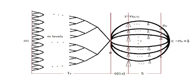
We will construct a graph based again on the example presented in [2]. For $T_{0}$ we will consider a binary tree of size $M$. The remaining part of the graph $B[0,z]\cup S$ will be the same with that of paradigm 2, as shown on figure 4.

We will determine $r,\gamma,\delta,m,M$ so that the conditions of Theorem 1.5 hold. As in the previous example we will start by placing conditions so that (H1) of Theorem 1.1 is not true. Since, in a binary tree

(4.15) $$\sqrt{Var_{\partial D}(\tau_{0})}\prec\mathbb{E}_{\partial D}(\tau_{0})$$

it is sufficient to have

(4.16) $$\mathbb{E}_{\partial D}(\tau_{0})>\mathbb{E}_{c}(\tau_{0})=6Nk.$$

Since from (4.2) we know that

$$m^{2}\lesssim\mathbb{E}_{\partial D}(\tau_{0})$$

we can choose

(4.17) $$m>\sqrt{Nk}.$$

As in paradigm 2, since the part $B[0,z]\cup S$ is common in the two examples, condition (C2) and

$$\gamma\sqrt{Var_{c}(\tau_{0})}\prec\mathbb{E}_{c}(\tau_{0})$$

for $\gamma=k^{p}$ with $p<\frac{1}{2}$ are satisfied. Similarly,

(4.18) $$t_{S}\prec 6Nk.$$

We will determine $s>0$ such that $\sqrt{\Phi}\leqslant n_{k}^{-s}$. Similarly to the previous example, it suffices to show that $\Phi=t_{S}\sum_{x\in S}\sum_{y\notin S}\mu_{S}(x)P(x,y)<n_{k}^{-2s}$. To determine parameters for $\Phi<n_{k}^{-2s}$ we compute

(4.19) $$\sum_{x\in S}\sum_{y\notin S}\mu_{S}(x)P(x,y)=\frac{2}{(2+r)\left|S\right|}$$

where the size of $S$ is

(4.20) $$\left|S\right|\asymp rN(\sum_{j\in\{[k/2],...,k\}}\frac{1}{n_{j}}).$$

Combining together (4.18), (4.19) and (4.20) we get

$$\Phi\asymp\frac{6Nk2(\sum_{j\in\{[k/2],...,k\}}\frac{1}{n_{j}})^{-1}}{(2+r)rN}\leq\frac{6k(\sum_{j\in\{[k/2],...,k\}}\frac{1}{n_{j}})^{-1}}{r}.$$

We can then choose

(4.21) $$r=6kn_{k}^{2s}(\sum_{j\in\{[k/2],...,k\}}\frac{1}{n_{j}})^{-1}.$$

Furthermore, we can request for $s$ to be sufficiently large so that

$$n_{k}^{s}>\frac{m^{3}}{6kN}>\frac{\sqrt{Nk}}{6Nk}=\frac{1}{6}k^{1/2}n_{k}^{1/2}$$

for large $k$. From the last one and the right hand side of (4.2) $\mathbb{E}_{\partial D}(\tau_{0})<m^{3}$, we obtain

(4.22) $$\frac{\mathbb{E}_{c}(\tau_{0})}{\sqrt{\Phi}}>\mathbb{E}_{\partial D}(\tau_{0}).$$

Concerning (C1) we require (4.10): $\left|S\right|+\left|B[0,z]\right|\prec\left|T_{0}\right|$. We have

$$\left|S\right|+\left|B[0,z]\right|\asymp rN(\sum_{j\in\{[k/2],...,k\}}\frac{1}{n_{j}})=6n_{k}^{2s}kN$$

where above we used (4.21). Since the size of he binary tree $T_{0}$ is $|T_{0}|=M$ for (4.10) we need $M\asymp e^{m}$, i.e. $m$, large enough so that

$$n_{k}^{2s}kN\prec M.$$

Concerning (C3), both assertions are trivially true. For inequality (H)(b) we can compute

$$\mathbb{E}_{\partial D}(\tau_{0})+\mathbb{E}[L]\mathbb{E}[\lambda_{i,j}]+\mathbb{E}[L]\mathbb{E}[\theta_{i}]\prec m^{3}$$

and

$$\frac{\gamma\sqrt{Var_{c}(\tau_{0})}}{\sqrt{\Phi}}=n_{k}^{s}k^{p+\frac{1}{2}}N.$$

From the last two we obtain (H)(b) for $s$ large enough such that $m^{3}<n_{k}^{s}k^{p+\frac{1}{2}}N$. It remains to show the following two inequalities.

$$\mathbb{E}_{\partial D}(\tau_{0})\prec\delta\ \sqrt{Var_{\partial D}(\tau_{0})}$$

and

$$\mathbb{E}_{c}(\tau_{0})\leq\delta\ \sqrt{Var_{\partial D}(\tau_{0})}\leq\frac{\mathbb{E}_{c}(\tau_{0})}{\sqrt{\Phi}}.$$

However, since (4.15), (4.16) and (4.22) hold, for the last two inequalities to be true we need to choose $\delta$ in the following range

$$\frac{\mathbb{E}_{\partial D}(\tau_{0})}{\ \sqrt{Var_{\partial D}(\tau_{0})}}<\delta<\frac{\mathbb{E}_{c}(\tau_{0})}{\sqrt{\Phi}\ \sqrt{Var_{\partial D}(\tau_{0})}}.$$

References

- [1] Levin D. A., Peres Y. and Wilmer E. L. (2009) Markov chains and mixing times, American Mathematical Society, Providence, RI.
- [2] Peres,Y. and Sousi P. (2015) Total variation cutoff in a tree. Ann. Fac. Sci. Toulouse Math, 4, 763-779.