Hybrid cluster+RG approach to the theory of phase transitions in strongly coupled Landau-Ginzburg-Wilson model

Abstract

It is argued that cluster methods provide a viable alternative to Wilson’s momentum shell integration technique at the early stage of renormalization in the field-theoretic models with strongly coupled fields because these methods allow for systematic accounting of all interactions in the system irrespective of their strength. These methods, however, are restricted to relatively small spatial scales, so they ought to be supplemented with more conventional renormalization-group (RG) techniques to account for large scale correlations. To fulfill this goal a “layer-cake” renormalization scheme earlier developed for rotationally symmetric Hamiltonians has been generalized to the lattice case. The RG technique can be naturally integrated with an appropriately modified cluster method so that the RG equations were used only in the presence of large scale fluctuations, while in their absence the approach reduced to a conventional cluster method. As an illustrative example the simplest single-site cluster approximation together with the local-potential RG equation are applied to simple cubic Ising model to calculate several non-universal quantities such as the magnetization curve, the critical temperature, and some critical amplitudes. Good agreement with Monte Carlo simulations and series expansion results was found.

I Introduction

Modern theory of critical phenomena in field-theoretic systems is based on the perturbative treatment of the Landau-Ginzburg-Wilson (LGW) model with weakly interacting fluctuating fields.Wilson and Kogut (1974); Le Guillou and Zinn-Justin (1980); Zinn-Justin (2002); Bagnuls and Bervillier (1985); Bagnuls et al. (1987) The theory is adequate in the critical region, at least in the space dimensions sufficiently close to four, where the interactions become weak at the late stages of the renormalization irrespective of whether the initial interactions were weak or strong.Wilson and Kogut (1974) In the latter case, however, the numerical values of the majority of non-universal quantities,—such as the critical temperatures and critical amplitudes,—remain largely unknownBagnuls and Bervillier (1985); Bagnuls et al. (1987) because non-perturbative field-theoretic techniques that are necessary to treat the strong coupling case are much less reliable than the perturbation theory.

There exist, however, strongly-coupled LGW-type models of considerable practical importance. For example, the Ising model that is widely used in the description of alloy thermodynamics (see Ref. Ducastelle, 1991 and references therein) can be cast in the form of strongly coupled LGW model, as will be discussed in Section II below. Therefore, the quantitative theory of critical phenomena in strongly coupled LGW-type models could be used, in particular, in prediction of alloy’s phase diagrams on the basis of ab initio band-structure calculations. Sanchez et al. (1984); Ducastelle (1991); Ducastelle and Gautier (1976); Wolverton et al. (1991); Zunger (1994); Zarkevich and Johnson (2004)

In terms of the RG theory a major obstacle hampering a fully quantitative description of critical phenomena in the strong coupling case lies in the absence of reliable methods of renormalization during the so-called transient regime that takes place at the early stage of the renormalization procedure.Wilson and Kogut (1974) The aim of the present paper is to suggest a technique that would combine two non-perturbative methods, namely, the cluster method of Refs. Tokar, 1983, 1997; Tan and Johnson, 2011 and the “layer-cake” renormalization scheme in the local potential approximation (LPA) Tokar (1984); Bervillier (2013) appropriately modified in such a way that the RG treatment would be invoked only when the system develops long-range correlations while away from the criticality a simpler cluster technique would be sufficient.

The material below is distributed as follows. In the next section the models, basic equations and notation will be introduced; besides, with the help of the field-theoretic diffusion RG equationsHori (1952) qualitative picture of the renormalization in the strong-coupling regime will be discussed. In Section III the cluster plus RG (C+RG) technique will be introduced and the simplest single site cluster approximation (SSA) presented as an input to the “layer-cake” RG approach which is explained in Section IV. Furthermore, in Section IV the LPA RG equation will be derived as a natural complement of the SSA and in Section IV.1 the formulas for some thermodynamic quantities in the SSA+LPA approach will be derived. In Section V the LPA equation derived in the previous section is transformed to the form that facilitates its numerical solution. In Section V.1 the approach will be illustrated by the description in the framework of the SSA+LPA of the ferromagnetic ordering in the simple cubic (SC) Ising model in zero magnetic field. In Section VI brief discussion of the results obtained and some concluding remarks will be given.

II The models and the diffusion RG equations

In this paper we consider the standard LGW model and the Ising model as its concrete realization. The LGW Hamiltonian for the fluctuating field $\phi$ is

$$H[h]=\frac{1}{2}\sum_{i,j}\phi_{i}G^{-1}_{ij}\phi_{j}+U[\phi]-\sum_{i}h_{i}\phi_{i},$$ (1)

where $i,j$ are indexes of the lattice sites and $U$ is the functional describing all interactions that are not written down explicitly in the equation. It also includes an arbitrary term of the form $-\frac{1}{2}\sum_{i,j}\phi_{i}r_{ij}\phi_{j}$ that also enters in the inverse of the pair correlation function (CF) in the first sum in Eq. (1) but with opposite sign, so that $H$ does not depend on $r$. In the quasi-momentum representation the pair CF reads

$$G({\bf k})=\frac{1}{\epsilon({\bf k})+r({\bf k})},$$ (2)

where for convenience the Fourier-transformed “bare” intersite interaction will be chosen in such a way that

$$\epsilon({\bf k})|_{\bf k\to 0}\sim Kk^{2}.$$ (3)

This can always be achieved by adding and subtracting a constant to/from the two terms in the denominator in Eq. (2); $K$ in Eq. (3) is some proportionality constant. In the case of the Ising model with interaction $J$ between nearest-neighbor (NN) spins on the SC lattice that we are going to use in our numerical calculations throughout the paper

$$\epsilon({\bf k})=2K(3-\cos k_{x}-\cos k_{y}-\cos k_{z}),$$ (4)

where

$$K=J/k_{B}T.$$ (5)

Finally, the last term in Eq. (1) describes the interaction with both real and fictitious (“source”) external fields. This slightly differs from the cluster approach of Refs. Tokar, 1983, 1985, 1997; Tan and Johnson, 2011 where the physical field and the source field were treated separately, though formally they are indistinguishable because they enter into the formalism as the sum

$$h_{i}=h_{i}^{ext}+h_{i}^{sorce}.$$ (6)

The reason for this modification of the formalism is that the present paper is devoted mainly to the RG approach though the cluster part will remain practically unchanged. But the magnetization in the RG part will be treated differently from the cluster part, namely, via the Legendre transform for the reasons explained below in section III.1.

To simplify notation, the energy unit will be chosen in such a way that the Boltzmann factor $1/k_{B}T$ were equal to unity. In this case the physical temperature in the system can be controlled by a value of some Hamiltonian parameter. In the calculations below we will use the inverse of the parameter $K$ from Eqs. (3), (4), and (5) as our dimensionless temperature.

In this notation the generating functional of the CFs reads

$$Z[h]=\int\prod_{i}d\phi_{i}e^{-H}.$$ (7)

The partition function is obtained from $Z[h]$ by setting $h$ to be equal to the external field $h^{ext}$. As is seen from Eq. (6), this is equivalent to the conventional route of setting the fictitious source field to zero. Tokar (1985, 1984, 1997).

Now with the use of the standard transformations Tokar (1985, 1984, 1997); Vasiliev (1998); Tan and Johnson (2011) the generating functional can be cast in the form

$$Z[h]=\left(\det G\right)^{1/2}\exp\left(\frac{1}{2}hGh\right)R[Gh],$$ (8)

where the generating functional of the S-matrix isHori (1952)

$$R[\phi]=\exp\left(\frac{1}{2}\frac{\partial}{\partial\phi}G\frac{\partial}{\partial\phi}\right)e^{-U[\phi]}$$ (9)

For simplicity, in Eqs. (8) and (9) and below we omit summations over the site indexes by adopting vector-matrix notation in the $N$-dimensional space ($N$ is the number of lattice sites) by treating fields as vectors and pair CFs as matrices.

As is easily seen from Eqs. (8) and (9), from the assumption that $G$ is the exact correlation function of the system it follows that Tokar (1983, 1985, 1997)

$$\left.\frac{\delta^{2}\ln R[\phi]}{\delta\phi_{i}\delta\phi_{j}}\right|_{\phi=Gh^{ext}}=0.$$ (10)

Similar to the cluster approach of Refs. Tokar, 1983, 1985, 1997; Tan and Johnson, 2011, this equation will constitute the self-consistency condition for the calculation of $r({\bf k})$. In the present paper we restrict ourselves to the smallest one-site “clusters” and to the SSA in the cluster part of the C+RG approach; the RG part will be treated in the LPA—the approximation with quasimomentum-independent vertexes, so $r$ in our explicit calculations will be just some non-negative number.

II.1 Diffusion RG equations

In the functional formalism Hori (1952); Wilson and Kogut (1974); Vasiliev (1998); Tokar (1984) the renormalization (semi)group can be introduced by representing $G$ in Eq. (9) as an integral over some evolution parameter $t$:

$$G=\int_{t_{0}}^{t_{1}}dtG_{t}(t).$$ (11)

(Here and below the subscripts corresponding to continuous variables will denote partial derivatives with respect to these variables.) With the use of the representation Eq. (11) it is easy to see that the functional Eq. (9) can be found as the solution of a Cauchy problem for the evolution equation for the group generator that in our case takes the form of the diffusion equation Hori (1952)

$$R_{t}[\phi,t]=\frac{1}{2}\frac{\delta}{\delta\phi}G_{t}\frac{\delta}{\delta\phi}R[\phi,t]$$ (12)

with the initial value

$$R[\phi,t_{0}]=\exp(-U[\phi]).$$ (13)

In principle, any parametrization satisfying Eq. (11) can be used Eq. (12). For example, in Ref. Hori, 1952 a straightforward parametrization was proposed consisting (in our notation) in multiplication of $G$ by $0\leq t\leq 1$

$$G({\bf k},t)=G({\bf k})t$$ (14)

so that $G_{t}=G$. This time-independence of the “diffusion constant” allows one to represent the solution of the diffusion equation Eq. (12) as the convolution of the initial field distribution Eq. (13) with the fundamental solution

$$P[{\bf\phi-\phi^{\prime}},t]=\prod_{\bf k}\frac{1}{[4\pi tG_{t}({\bf k})]^{N/2}}\exp\left(-\frac{(\phi-\phi^{\prime})_{\bf-k}(\phi-\phi^{\prime})_{\bf k}}{4tG_{t}({\bf k})}\right).$$ (15)

For our purposes it is important to note that in the vicinity of the critical point $G_{t}=G({\bf k})$ at small $|{\bf k}|$ is positive and large. As we know from the properties of the conventional diffusion, even the delta-function-like initial probability density distributions that in our case would describe infinitely strong interactions in Eq. (13) can be strongly smeared, given sufficient time and sufficiently large diffusion constant. In our case this would mean diminishing of the interaction in the renormalized effective interaction $U$ in Eq. (13) to small values. It is to be stressed, however, that the smearing strongly depends on both the time of the diffusion and on the value of the diffusion constant, as can be qualitatively seen from the fundamental solution Eq. (15).

Thus, in order the interactions at a given ${\bf k}$ were small, the effective time–diffusion constant product $tG_{t}({\bf k})$ in Eq. (11) should be large. The success of the RG approach to critical phenomena is essentially based on the fact that this condition is satisfied in the vicinity of the critical point, at least in the systems of dimension close to four.Wilson and Kogut (1974) For example, in Eq. (14) time varies only from 0 to one. But $G_{t}$ along the path leading to the singularity at ${\bf k=0}$ remains very large, in fact, infinite at the criticality. Thus, the product $tG_{t}$ can be very large. However, away from ${\bf k=0}$ and/or away from the criticality the interactions in $U$ in Eq. (13) may turn out to be too large to be smeared by the kernel Eq. (15) to sufficiently broad probability distribution. In this case renormalized interactions will remain strong and non-perturbative techniques are necessary to deal with them.

One may wonder whether the simple parametrization Eq. (14) with all quasimomenta being treated equally is adequate for discussion of renormalization in the critical region where the long-wavelength fluctuations are the most important ones. In Wilson’s original approach the renormalization process proceeds via a different route when the short-wavelength fluctuation are being integrated out completely with the long-wavelength field components left intact.Wilson and Kogut (1974) To see that all renormalization trajectories defined by the parametrization in Eq. (11) are physically equivalent, let us consider a simple case of a smooth cutoff when large-quasimomenta components are integrated out faster than the long wave-length ones, as is done in many renormalization schemes Bogoli︠u︡bov and Shirkov (1959); Wilson and Kogut (1974); Polchinski (1984). For example, the Pauli–Villars regularization Bogoli︠u︡bov and Shirkov (1959) can be obtained within our approach with the use of parametrization

$$G_{t}({\bf k},t)=\frac{1}{[\epsilon({\bf k})+r({\bf k})+t]^{2}}.$$ (16)

Integrating this from $t=0$ to some sufficiently large value of $t$ one gets

$$G({\bf k},t)=\frac{1}{\epsilon({\bf k})+r({\bf k})}-\frac{1}{\epsilon({\bf k})+r({\bf k})+t}$$ (17)

In the critical region and at small ${\bf k}$ the denominator in the first term on the right hand side of Eq. (2) is small at small ${\bf k}$, so in this case $G({\bf k},t)\approx G({\bf k})$. However, as $\epsilon({\bf k})+r({\bf k})$ grows towards and past the value of $t$, $G({\bf k},t)$ becomes small thus effectively cutting off short-wavelength fluctuations in $G({\bf k})$ qualitatively similarly to the Wilson’s method. From the integrated Eq. (16) one sees that in case of finite cutoff in $k$-space large values of $t$ larger than some finite value $t_{1}$ give contribution into Eq. (11) of $O(1/t_{1})$ so for qualitative reasoning they can be neglected. The interval $[0,t_{1}]$ can be mapped onto interval [0,1], so qualitatively the problem reduces to the previously considered case.

This qualitative reasoning was meant to qualitatively substantiate the observation that the structure of strongly coupled LGW models is such that during the renormalization flow the system either enters into critical regime with weak coupling or retains the strong interactions but with only short-range correlations. This dichotomy should justify the need for the hybrid approach when strong coupling short-range behavior is treated within cluster approximations that are known to be well suited to this kind of problems while the critical behavior is dealt with in an RG technique that is the only viable approach to the problem in field-theoretic models.

Of course, not all LGW-type statistical models are strongly coupled but some practically important ones may have effective interactions even of infinite strength. For example, the Ising model can be transformed into a field-theoretic system as follows

$$Z[h]=\mbox{Tr}_{s_{i}=\pm 1}\exp\left(\frac{1}{2}\sum_{ij}s_{i}J_{ij}s_{j}+\sum_{i}h_{i}s_{i}\right)$$

$$=\int\prod_{i}[d\phi_{i}2\delta(\phi_{i}^{2}-1)]\exp\left(\frac{1}{2}\sum_{ij}\phi_{i}J_{ij}\phi_{j}+\sum_{i}h_{i}\phi_{i}\right),$$ (18)

where the interaction can be represented as infinitely strong $\lambda\phi^{4}$ coupling if the delta-functions in Eq. (18) are represented as

$$\delta(\phi_{i}^{2}-1)=\left.C_{\lambda}e^{-\lambda\sum_{i}(\phi_{i}^{2}-1)^{2}}\right|_{\lambda\to\infty},$$ (19)

($C_{\lambda}$ is a normalization constant).

The Ising model is being widely used, inter alia, in the study of alloy thermodynamics. Sanchez et al. (1984); Ducastelle (1991); Ducastelle and Gautier (1976); Wolverton et al. (1991); Zunger (1994); Zarkevich and Johnson (2004) Therefore, the development of efficient techniques of its solution with realistic interatomic/interspin interactions is a problem of considerable practical interest. This problem has been extensively studied in the past decades and sophisticated techniques has been developed that predict non-critical behaviors with high accuracy (see Refs. Ducastelle, 1991; Tokar, 1997; Tan and Johnson, 2011 and references therein). The critical behavior, however, was investigated only in simple model systems Pelissetto and Vicari (2002) while in the theory of alloys the second order phase transitions are usually treated either within the cluster variation method to which the mean-field critical behavior is inherent (see Ref. Ducastelle, 1991 for extensive bibliography) or with the use of the Monte Carlo (MC) simulations.

III C+RG method

In the functional cluster technique of Refs. Tokar, 1983, 1985, 1997; Tan and Johnson, 2011 one can calculate with good accuracy only the critical temperature while the critical behavior in general is described very poorly (see, e. g., Fig. 1). This approach, however, is based on the field-theoretical formalism so in principle should be compatible with Wilson’s RG techniques. The rest of the present paper will be devoted to the realization of this observation in application to the strongly coupled LGW model with the use of the SC Ising model in concrete calculations.

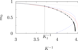
Figure 1: (Color online) Solid line: $K^{-1}$ below $K^{-1}_{1}$—solution of the SSA Eqs. (24) and (25); $K^{-1}$ above $K^{-1}_{1}$—least square fitted cubic splineDierckx (1993) to the black dots obtained from the solutions of the LPA RG Eq. (57); $K^{-1}_{1}$ is the dimensionless temperature where the two solutions matched. Dashed curve: the MC simulation data from Ref. Talapov and Blöte, 1996. Dash-dotted line: solution of the SSA equations. Dotted curve: Two leading terms of the low temperature expansion from Ref. Bhanot et al., 1992.

The cluster approach we will use is a systematic technique to treat lattice field-theoretic models and is well documented in previous publications, so here it will only be mentioned why it is insufficient to the description of the second order phase transitions. The essence of the approach is easier to explain using the coarse-grained version Tan and Johnson (2011) of the cluster method though non-coarse-grained version may be more accurate Tokar (1983, 1997).

In the cluster approach one tries to approximate an infinite system of strongly coupled fields with a finite cluster of size $N_{c}$. The reason is that the calculation of the partition function Eq. (7) can be approximately reduced to $N_{c}$-dimensional integral that can be calculated exactly irrespective of the strength of the interactions. In Fig. 2 is drawn a cross-section of the CF $G({\bf k})$ in the first Brillouin Zone (BZ) of a $d$-dimensional cubic lattice along the $k_{x}$ axis. Let us imagine that the system is divided into clusters of size $N_{c}=4^{d}$ sites. The BZ of such a system will shrink correspondingly (see vertical lines). But because the system remains the same we will keep the initial BZ divided into $4^{d}$ parts to simplify the discussion. In the coarse-grained approximation $G({\bf k})$ is approximated by its average value within each sub-cell (the horizontal lines in Fig. 2) and thus $N$ ${\bf k}$-points in the BZ are replaced by a finite number $N_{c}$ of the points (for the details see Refs. Tan and Johnson (2011); Maier et al. (2005)). The accuracy of the cluster approximation can be estimated by the size of the deviation of the exact $G({\bf k})$ from its average values within the subcells. It is expected that with the growth of $N_{c}$ the cluster approximation will be converging to the exact solution as long as the Riemann sum over subcells will be converging towards the exact integral.

Figure 2: Schematic picture of the separation of $G$ in Eqs. (20) and (21) into $\bar{G}$—thick solid lines below $t_{0}$ plus solid ${G}=t_{0}$ line segment and $\bar{G}$—solid lines above the ${G}=t_{0}$ line. Shown also are the average values of the coarse-grained correlation function (horizontal thin solid lines).Maier et al. (2005); Tan and Johnson (2011) Vertical dashed lines are the boundaries that divide the initial Brillouin zone into smaller parts when the system is divided into clusters having four cells in the $x$-direction.

The Riemann sum, however, does not converge in the case of improper integrals,Weisstein in particular, when the integrand diverges, as is the case with $G({\bf k})$ at the critical point when $G({\bf k\to 0})\to\infty$. In this case for an arbitrarily small integration cell surrounding the point ${\bf k}=0$, the deviation of the exact $G({\bf k})$ from the average CF will be arbitrarily large at a point ${\bf k}$ sufficiently close to zero.

This necessitates introduction in the vicinity of the critical point of some other integration technique. To this end, let us first separate the singular part of $G({\bf k})$ near ${\bf k\approx 0}$ from the nonsingular behavior at other values of ${\bf k}$ as

$$G({\bf k})=\bar{G}({\bf k})+\hat{G}({\bf k}),$$ (20)

where

$$\begin{array}[]{l|c|c}&{G}({\bf k})\leq t_{0}&{G}({\bf k})>t_{0}\\ \hline\cr\bar{G}({\bf k})=&{G}({\bf k})&t_{0}\\ \hline\cr\hat{G}({\bf k})=&0&{G}({\bf k})-t_{0}\end{array}$$ (21)

(see Fig. 2). It is easy to see that by construction the variation of $\bar{G}({\bf k})$ is always bounded so the Riemann sum converge and the problem can be efficiently treated within the cluster approach. It is to be noted that far from criticality $r$ in Eq. (2) can be is large and $G({\bf k})<t_{0}$. In this case the C+RG approach reduces to purely cluster approach of Refs. Tokar, 1983, 1997; Tan and Johnson, 2011. But when the second term in Eq. (20) is non-zero, the cluster solution should be augmented with the RG part. The latter will be considered in the next section while in the rest of this section we will illustrate the cluster part of the technique with the simple example of the Ising model in zero external field in the SSA.

III.1 SSA in application to the Ising model

In the SSA the average over ${\bf k}$ is performed over the whole Brillouin zone and therefore the result is equal to the site-diagonal element of the truncated correlation function:

$$\frac{1}{N}\sum_{\bf k}\bar{G}({\bf k})=\bar{G}_{ii}$$ (22)

In the present paper we will be interested mainly in the second order phase transition from the paramagnetic to ferromagnetic state in the absence of external magnetic fields. The conventional SSA Tokar (1983, 1985, 1997); Tan and Johnson (2011) consists in approximating matrix $G$ in Eq. (9) by its diagonal elements in which case the calculation of $R$ reduces to the calculation of 1D integrals. But before that one shifts the integration variables in Eq. (7) by the (unknown) value of the spontaneous magnetization $m$, so the effective potential in the SSA reads Tokar (1985, 1997); Tan and Johnson (2011)

$$U^{SSA}[\phi,m]=\sum_{i}\left(\bar{G}_{ii}^{-1}\phi_{i}^{2}/2+m\bar{G}_{ii}^{-1}\phi_{i}-\ln\cosh[\bar{G}_{ii}^{-1}\phi_{i}+(\bar{G}_{ii}^{-1}-r)m]\right)+NC,$$ (23)

where $C$ does not depend on field $\phi$ and so its explicit value will not be needed in our present calculations. In case of necessity it can be easily derived or obtained from the formulas of Ref. Tokar, 1997.

In the ordered phase the SSA Eq. (23) is good at low temperatures where the two degenerate ground states with magnetizations $\pm m_{0}$ are energetically well separated, so the state represents a background of spins directed in one directions plus rare and small clusters of oppositely directed spins.

In the critical region, however, the picture is different. Large clusters of spins of both directions are almost equal in size with only slight bias toward one direction.Wilson and Kogut (1974) In this case the description of the system with the use of the average magnetization $m_{0}\approx 0$ does not represents well the physics of the spontaneous symmetry breaking. Therefore, in our RG approach we will use Eq. (23) with $m=0$ both in the symmetric and the ordered phase and calculate the spontaneous magnetization via the Legendre transform.Zia et al. (2009); Vasiliev (1998)

To be more specific, let us assume for the moment that the cut-off $t_{0}$ is infinitely large so the RG part is not necessary. In this case the problem is solved in the SSA as follows.Tokar (1985, 1997) First, equating to zero the first derivative of Eq. (23) with respect to $\phi_{i}$ the SSA equation for the equilibrium magnetization $m_{0}$ is obtained:

$$m_{0}=\tanh\left[\left(G^{-1}_{ii}-r\right)m_{0}\right]$$ (24)

then Eq. (10) for $\phi=0$ gives

$$G_{ii}+m_{0}^{2}=1$$ (25)

and the SSA magnetization is shown in Fig. 1. As can be seen, when close to the saturation value $m=1$, the SSA agrees well with the low-temperature expansion. It can be shown analytically that Eqs. (24)–(25) reproduce exactly its two leading terms.

From Fig. 1 one can see that close to the critical point, however, the SSA solution exhibits behavior that is very far from the correct one as seen, e. g., in the MC simulations.Talapov and Blöte (1996) Therefore, in this region the cluster approximation breaks down and should be replaced with more adequate treatment.

To apply the C+RG approach one has first to decide on the value of the cut-off $t_{0}$ to be used in the calculations. Assuming that SSA gives reasonably accurate solution in the non-critical region, let us use it in assessing the Ginzburg criterion by comparing the square of the long-wavelength fluctuations of the order parameter with the mean order parameter squared asGould and Tobochnik (2010)

$$\mbox{Gi}\sim\frac{(\Delta m)^{2}}{m_{0}^{2}}=\frac{G({\bf k\to 0})}{m_{0}^{2}}=\frac{1}{rm_{0}^{2}}.$$ (26)

Assuming further that the critical region starts at the point where $\mbox{Gi}\approx 1$, one finds with the use of the SSA solution that at this point (marked by the subscript 0) $1/K_{0}\approx 3.9$ and $t_{0}=1/r_{0}=0.65$—the value we will use in calculations throughout the paper. In section V.1 we will show that the results obtained weakly depend on the choice of the parameter.

IV Layer cake renormalization scheme and the LPA

Thus, having assumed that in the critical region the SSA can satisfactorily describe only those fluctuations whose correlation do not exceed some value $t_{0}$, we also have to develop an RG approach that would take into account those fluctuations. Formally we need to calculate an expression similar to Eq. (9) but this time with the effective potential Eq. (23) renormalized by the SSA. To this end it is convenient to rewrite the diffusion RG Eq. (12) through the logarithm of the S-matrixHori (1962) or the effective potential $U[\phi,t]=-\ln R[\phi,t]$ which we assume can be expanded in the functional Taylor series in the field $\phi$ as

$$U=N\sum_{n,\{\mathbf{k}_{j}\}}N^{-n/2}u_{n}(\{\mathbf{k}_{j}\},t)\delta\left(\sum_{j=1}^{n}\mathbf{k}_{j}\right)\prod_{j=1}^{n}\phi_{\mathbf{k}_{j}}.$$ (27)

In terms of $U$ Eq. (12) reads

$$U_{t}[\phi,t]=\frac{1}{2}\sum_{\bf k}G_{t}({\bf k},t)\left(\frac{\partial^{2}U}{\partial\phi_{-\bf k}\partial\phi_{\bf k}}-\frac{\partial U}{\partial\phi_{-\bf k}}\frac{\partial U}{\partial\phi_{\bf k}}\right).$$ (28)

In the layer cake renormalization schemeTokar (1984) the CF $G$ is represented as the sum of infinitesimal layers of thickness $dt$ which when stacked together will form the function under consideration (see, e. g., Fig. 1 in Ref. Tokar, 1984). It is easy to see that this leads to

$$G_{t}({\bf k},t)=\theta\left[G({\bf k},t)-t\right],$$ (29)

where $\theta$-function plays the role of the indicator functionlay (see Appendix A). On substituting this in Eq. (28) together with the expansion Eq. (27) one should note a subtle difference between the two summations over $\mathbf{k}$ present in the equation. The second summation consists of terms proportional to the product of two lattice delta-functions (Kronecker symbols)

$$\sum_{\bf k}\theta\left[G({\bf k},t)-t\right]\delta\left(\sum_{j=1}^{n-1}\mathbf{k}_{j}-\mathbf{k}\right)\delta\left(\mathbf{k}+\sum_{j^{\prime}=1}^{n^{\prime}-1}\mathbf{k^{\prime}}_{j^{\prime}}\right)u_{n}(\{\mathbf{k}_{j}\}_{i},\mathbf{-k},t)u_{n^{\prime}}(\{\mathbf{k}^{\prime}_{j^{\prime}}\}_{i^{\prime}},\mathbf{k},t)$$ (30)

and thus can be performed formally exactly in each term by simply substituting $\mathbf{k}$ by, say, $\sum_{j=1}^{n-1}\mathbf{k}_{j}$ in all factors entering the product. (The subscripts $i,i^{\prime}$ in Eq. (30) means that corresponding quasimomentum in the set is absent because it is set to be equal to $\pm\mathbf{k}$; these same terms reduce by unity the summations over $j,j^{\prime}$ in the arguments of the delta-functions.) The first summation in Eq. (28), however, contains only one delta-function

$$\frac{1}{N}\sum_{\bf k}\theta\left[G({\bf k},t)-t\right]\delta\left(\sum_{j=1}^{n-2}\mathbf{k}_{j}+\!\not{\mathbf{k}}-\!\not{\mathbf{k}}\right)u_{n}(\{\mathbf{k}_{j}\}_{ii^{\prime}},\mathbf{k},\mathbf{-k},t)$$ (31)

so that to carry out the summation one needs to know explicitly the dependences of the vertex functions on quasimomenta.

Thus, Eq. (28) is a complicated nonlinear integro-differential equation with infinite number of variables and its solution presents a formidable task. It can be considerably simplified, however, in the LPA that consists in first setting to zero all $\phi_{\bf k}$ with ${\bf k}\not=0$ outside the contour defined by the level set $G({\bf k})=t$. This is legitimate because in our problem only the homogeneous fields with ${\bf k}=0$ survives after the substitution $\phi=Gh^{ext}$ in Eq. (10). After that we assume that the vertex functions $u_{n}$ are independent of the quasimomenta, so that the functional Eq. (27) can be mapped onto the function Tokar (1984)

$$u(x,t)=\sum_{n}u_{n}(t)x^{n}.$$ (32)

The approximations should be good in the critical region where small quasimomenta dominate so that Eq. (32) approximates Eq. (27) as

$$u_{n}(t)\approx u_{n}(\{\mathbf{k}_{j}\},t)|_{\{\mathbf{k}_{j}\}\to 0}$$ (33)

and

$$x\approx\phi_{\mathbf{k}\to 0}$$ (34)

With these approximations it is easy to see that $\theta[G({\bf k\to 0},t)]=1$ in Eq. (30) and the sum in Eq. (31) can be calculated exactly to give

$$u_{t}=\frac{1}{2}\left[s(t,r)u_{xx}-u_{x}^{2}\right],$$ (35)

where

$$s(t,r)=n_{SC}(t^{-1}-r)$$ (36)

and $n_{SC}(E)$ is the integrated density of states with the dispersion law given by Eq. (4) (see Appendix A).

In Fig. 3 the physical meaning of the function $s$ from Eq. (35) is explained. One can see, in particular, how the present approach differs from the usually studied LPA for RG equations in the scaling form. Tokar (1984); Bervillier (2013); Caillol (2012) The latter is obtained by substituting into Eq. (68) $D(E)\propto\sqrt{E}$ which is the universal behavior for 3D systems (see the square root curve in Fig. 3). Fig. 3 also illustrates why the conventional perturbative RG is insufficient for the calculation of non-universal quantities. While higher powers of $k_{x,y,z}$ can be neglected in the conventional RG approach due to their smallness,Wilson and Kogut (1974) in our case function $s$ contains the van Hove singularities that appear only when all powers of $k_{x,y,z}$ are kept in the expression for $s$ because the NN interaction in Eq. (4) that are analytic in ${\bf k}$ have to be summed to infinite orders to exhibit the singular behavior.

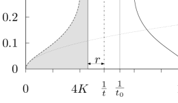
Figure 3: Density of states for the SC lattice. The area of the shaded region is equal to $s(t)$ in Eqs. (35) and (57). The dotted curve corresponds to the universal square-root scaling behavior observed at small $E$ and extended on all region of allowed values of $E$.

Thus, by means of the function $s$ the LPA Eq. (35) is capable of accounting for all pair interactions that are usually considered to be the most important ones in alloys. Sanchez et al. (1984); Ducastelle (1991); Ducastelle and Gautier (1976); Wolverton et al. (1991); Zunger (1994); Barrachin et al. (1994); Zarkevich and Johnson (2004) But the aim of the C+RG is to account for all cluster interactions in the system. The cluster part of the method is well suited for this purpose but the RG part needs some adjustment. It is to be noted that only quasimomentum-dependent part of cluster interactions poses problems because the constant part is accounted for in the $u_{n}(\{\bf k_{j}\to 0\})$ local potential.

A straightforward approach would be to augment the LPA equation Eq. (35) with RG equations for the coefficients of expansion of the vertex functions in powers of the quasimomenta.Wilson and Kogut (1974) The ensuing equations, however, will be rather cumbersome. Wilson and Kogut (1974) So, presumably, it would be easier to push the initial quasimomentum cutoff $k_{0}\sim 1/\sqrt{t_{0}}$ to as small value as possible. This would justify the neglect of the quasimomentum dependence of most of the vertexes with the possible exception of the corrections into the pair ones which are responsible for index $\eta$. There are two ways to diminish $k_{0}$. First, to enlarge the cluster in the first part of the calculation to make the BZ possibly smaller and then to chose maximally large $t_{0}$. Large $t_{0}$ will diminish the error due to the neglect of the ${\bf k}$-dependence of the vertex functions but will enlarge the error in the cluster part because of larger deviation of $G({\bf k})$ from its mean value in the cell. Thus, some optimum choice should exist which will depend on the presence and the size of non-pair effective cluster interactions in the system. In Section V.1 we will show that the choice of $t_{0}$ only weakly influences the results at the SSA+LPA level, so it can be used to improve more advanced calculations with larger clusters and/or better RG equations. As can be seen from Eq. (23) at $m=0$, the interaction terms are even powers of $\phi_{i}/\bar{G}_{ii}$

$$(\phi_{i}/\bar{G}_{ii})^{4}/12-(\phi_{i}/\bar{G}_{ii})^{6}/45+\dots,$$ (37)

so the smaller is the cutoff $t_{0}$, the smaller is $\bar{G}_{ii}$ hence, larger the interaction. For example, the coefficient strength of the $\lambda\phi^{4}$ interaction at the critical point $1/K_{c}=4.44$ and cutoff $t_{0}=0.65$ is

$$\lambda=[12\bar{G}_{ii}^{4}(2K_{c})^{2}]^{-1}\approx 3.2$$ (38)

where $\bar{G}_{ii}|_{t_{0}=0.65}\approx 0.6$ and the $2K_{c}$ comes from the renormalization of the field $\phi$ necessary to bring our quadratic term $Kk^{2}|\phi_{\bf k}|^{2}$ in our Hamiltonian (see Eqs. (1) and (3)) to the canonical form $k^{2}|\phi_{\bf k}|^{2}/2$Wilson and Kogut (1974); Le Guillou and Zinn-Justin (1980). As we see, the coupling in the case $t_{0}=0.65$ is rather strong. This does not matter in the LPA that we use in the present paper because the RG equation was derived without any resort to the smallness of the couplings and thus can be applied to the strong coupling case of Eq. (38). However, the LPA is not easy to improve in the nonperturbative manner to exhibit, for example, more accurate critical behavior with improved indexes.Bervillier (2013) Therefore, it would be more practical to push the cutoff $t_{0}$ higher in which case $\bar{G}_{ii}$ will approach unity (see Eq. (25) with $m_{0}=0$) and the coupling in Eq. (38) will tend to much smaller value $\lambda\approx 0.4$. This should facilitate application of perturbative techniques.Wilson and Kogut (1974); Le Guillou and Zinn-Justin (1980); Zinn-Justin (2002); Bagnuls and Bervillier (1985); Bagnuls et al. (1987)

Of course, the omission of nonlocal contributions even at large $t_{0}$/small $k_{0}$ values will still introduce some errors into the results. But it should be remembered that the cluster part of the calculations will always be of restricted accuracy because the complexity of the calculations grows exponentially with the cluster size, so the size will be bounded by some finite value of the order of those used in the calculations of Ref. Tan and Johnson, 2011. So making the RG part much more accurate does not have much sense.

IV.1 Measurable quantities

With Eq. (35) the field-theoretic problem with infinite number of variables reduced to a Cauchy’s problem for the second-order evolution equation for a function of two variables. From Eqs. (23), (27), and (32) it is easy to derive the initial condition

$$u(x,t_{0})=\bar{G}_{ii}^{-1}x^{2}/2-\ln\cosh(\bar{G}_{ii}^{-1}x)+C$$ (39)

(we remind that in the RG part we set $m=0$ both above and below the critical temperature). The only peculiarity of our Cauchy problem is that it should be solved in a self-consistent manner to satisfy the condition Eq. (10):

$$u_{xx}(x=h/r,t=1/r)=0.$$ (40)

To calculate physical quantities from in the SSA+LPA we first need to find the per-site Gibbs potential

$$g=-\ln Z[h]/N$$ (41)

(we remind that $k_{B}T=1$ in our units). In the LPA the field $h_{i}$, that in principle could be used to calculate via the differentiation of $Z[h]$ all correlation functions, reduces to a single number—the value of the zero-momentum component, i. e., to the homogeneous external magnetic field $h$ (we will denote it by the same letter because from now on it will have only this meaning). So only homogeneous responses can be found within LPA. It is important to point out, however, that in the self-consistent approach the pair correlation function can also be calculated through Eqs. (2) and (40) because the first equation was derived before the local approximation was made.

With the use of Eq. (8) in the SSA+LPA approximation one gets

$$g(h)=-\frac{1}{2N}\ln\det G-\frac{h^{2}}{2r}+u(x=\frac{h}{r},t=\frac{1}{r}),$$ (42)

To find solutions with spontaneously broken symmetry, however, we need the Helmholtz free energy that can be obtained from the Gibbs potential in a standard way via the Legendre transform:Zia et al. (2009); Vasiliev (1998)

$$f(m)=g-hg_{h}=g+hm,$$ (43)

where the dependence of $h$ on magnetization $m$ is found from the definition

$$m=-g_{h}=x-u_{x}/r.$$ (44)

The magnetic susceptibility is

$$\chi=m_{h}=-g_{hh}=r^{-1}-u_{xx}/r^{2}=r^{-1},$$ (45)

where use has been made of the self-consistency condition Eq. (40). We note that in our approximation Eq. (45) agrees with another definition

$$\chi=G({\bf k=0})=1/r$$ (46)

so that at this level of approximation the approach is consistent.

The critical amplitudes $C^{\pm}$ describe the asymptotic behavior of the susceptibility in the vicinity of the critical point $K_{c}$ asLiu and Fisher (1989); Ruge et al. (1994); Pelissetto and Vicari (2002)

$$\chi\simeq C^{\pm}\tau^{-\gamma},$$ (47)

where

$$\tau=|K_{c}/K-1|$$ (48)

$\gamma$ is the critical index, and $\pm$ denotes whether the amplitude is being measured or calculated above (+) or below (-) the critical temperature. Now because $r$ in Eqs. (45) and (46) can be found from the solution of the SSA+LPA equations, the amplitudes in Eq. (47) can be calculated. Similarly, from the Fourier transform of Eq. (2) the correlation length can be found as

$$\xi=\sqrt{K/r}\simeq f^{\pm}\tau^{-\nu},$$ (49)

where $\nu$ is another critical index. From this relation the behavior of $r$ in the critical region can be derived as

$$r=a\tau^{2\nu},$$ (50)

where $a$ is a constant. Comparing this with Eq. (47) one can find $a=1/C^{\pm}$ and the relation between the exponents is

$$\gamma=2\nu.$$ (51)

This relation imply $\eta=0$Pelissetto and Vicari (2002) and is a consequence of the LPA.Tokar (1984)

Finally, the amplitude $B$ and the critical index $\beta$ are defined from the behavior of the spontaneous magnetization near the critical point as

$$m_{0}\sim B\tau^{\beta}.$$ (52)

These five amplitudes ($C^{\pm},f^{\pm}$ and $B$) together with the critical temperature will be the non-universal quantities that we will calculate within the C+RG approach in the present paper.

Eq. (35) is easily solvable numerically in the symmetric phase. So if we were interested only in critical amplitudes, we could solve Eqs. (35) and (40) in this phase to find $C^{+}$ and $f^{+}$ and then utilized known values of the universal ratios to calculate $C^{-}$, $f^{-}$ and even

$$B=\sqrt{Q_{c}C^{+}/f^{+}},$$ (53)

where $Q_{c}$ is a known universal quantity.Pelissetto and Vicari (2002) However, because our aim is to develop a method that would describe thermodynamics also beyond the critical region, we would like to solve the C+RG equations below the critical temperature as well. Unfortunately, Eq. (35) is not easily solvable in the ordered phase. Therefore, numerical calculations were performed with transformed equation that could be solved in both phases as explained below.

V Numerical solution of the LPA equation

Numerical solution of a Cauchy problem for equations similar to Eq. (35) is usually reduced to solution of a set of ordinary differential equations via the method of lines. Hamdi et al. (2007) In the disordered phase Eq. (35) can be quite efficiently solved with the use of this method but in ordered phase it becomes practically intractable, at least at the double precision arithmetics that was used in the calculations. Apparently, the reason for this lies in the RG nature of the equation. As such, Eq. (35) describes the renormalization of all Hamiltonians of the LGW type, in particular, the quadratic Hamiltonian corresponding to the exactly solvable Gaussian model.Wilson and Kogut (1974) In our formalism this shows itself in the existence of an exact solution of Eq. (35) of the form

$$u^{(G)}(x,t)=u_{2}x^{2}+u_{1}x+u_{0}.$$ (54)

As is known, the Gaussian model is pathological in that at negative $u_{2}$ it is not bounded from below and so does not possess an ordered state. So if one attempts integration of Eq. (35) with the initial $u^{(G)}(x,t_{0})$ having negative value of $u_{2}(t_{0})$, than the solution that can be obtained analytically in this case will have the form

$$u_{2}(t)=\frac{1}{2t+c_{0}},$$ (55)

where $c_{0}$ is a negative constant such that $1/(2t_{0}+c_{0})=u_{2}(t_{0})<0$. As we see, at some later time $t=-c_{0}/2$ Eq. (55) develops a non-integrable singularity $u_{2}\to\-\infty$ that cannot be treated within conventional finite-difference schemes. This is what was qualitatively observed in calculations. Obviously that negative $u_{2}(t=t_{0})$ are forbidden in the Gaussian model because the probability distribution became non-normalizable. But negative $u_{2}$ is exactly what drives the ordering in the interacting LGW model. The Hamiltonian is bounded from below due to quartic and higher terms so the initial condition with $u_{2}(t=t_{0})<0$ is what happens in reality. But in numerical calculations due to computational errors and the finite range of variation of $x$ the trajectory leading to unphysical solution is apparently very close to the physical trajectory so that their separation is numerically proved to be impossible.

In Ref. Bervillier, 2013 time-independent analogue of Eq. (35) in the scaling limit ($r=0,t\to\infty$, $s$ corresponding to the square root density of states) in scaling variablesTokar (1984) was studied at the critical point and also was found to be very difficult to deal with numerically. It was found, however, that a change of variables can significantly alleviate the difficulties. It turned out that with necessary modifications this change of variables can be helpful also in our case of time-dependent Eq. (35) in the non-scaling regime. Specifically, by introducing new independent variable $y$ and new function $v(y,t)$ as

$$y(x,t)=x-(t-c)u_{x}(x,t)$$ (56a)

$$v(y,t)=u(x,t)-{(t-c)}u_{x}^{2}/2,$$ (56b)

($c$ is an arbitrary constant) Eq. (35) can be cast in the form (see Appendix B)

$$v_{t}=\frac{s(t,r)v_{yy}}{2[1+(t-c)v_{yy}]}$$ (57)

with the self-consistency condition

$$v_{yy}=0$$ (58)

(see Eq. (71)). From Eq. (57) it is easy to see that the quadratic model of the kind of Eq. (54) but expressed in terms of the new variables does not exhibit any singularities because $\partial v_{2}(t)\partial t=0$ so the initial value of $v_{2}$ remains the same irrespective of its sign. This solves the problem of the singular second derivative and allows for numerical solution in both symmetric and ordered phases.

Equations similar to Eq. (57) were studied previously in LPA-RG approaches (see Refs. Bervillier, 2013; Caillol, 2012 and references therein) with some physical meaning being ascribed to the quantities similar to our $v$ and $y$. In our approach, however, such a meaning is not easily discernible so we will consider these entities as purely auxiliary variables while physical quantities will be calculated with the use of thermodynamic potentials introduced in previous section.

As is easily seen, the arbitrary constant $c$ in Eqs. (56) is convenient to chose to be equal to $t_{0}$. In this case at $t=t_{0}$ $y=x$ and $v=u$, so the initial function $v$ is the same as in Eq. (39) with only $x$ replaced with $y$. Thus, denoting the time span from the start to the end of the integration as

$$\Delta t=(1/r-t_{0})$$ (59)

with the use of Eqs. (42), (44), (45), (56), and Appendix B we can express all physical quantities in terms of the auxiliary variables as

$$x=h/r=y+\Delta tv_{y}$$ (60a)

$$u=v+\Delta tv_{y}^{2}/2$$ (60b)

$$m=y-t_{0}v_{y}$$ (60c)

$$f=g-xg_{x}=u-xu_{x}+rx^{2}/2$$ (60d)

$$\chi^{-1}=f_{mm}=r(1+\Delta tv_{yy})/(1-t_{0}v_{yy})=r,$$ (60e)

where in the last equality use has been made of the self-consistency condition Eq. (58).

V.1 SC Ising model in zero magnetic field

Because our major interest in the present paper is in the second-order phase transitions, we will restrict the solution of the Ising model to the $h=0$ case. In the symmetric phase $v(y,t)$ is a smooth symmetric function and its numerical solution is rather unproblematic. The difficult part of the problem was the self-consistent solution of Eqs. (57) and (58) in the ordered phase where the solution exhibited non-smooth behavior (see Fig. 4). Both the differential equation per se and the self-consistency requirement posed problems. In Ref. Caillol, 2012 the author resorted to quadruple-precision computations to reliably solve equations of this kind with the use of the method of lines. Unfortunately, in the present study such facilities were unavailable, so conventional double-precision arithmetic and the LSODE routine at the highest possible accuracy (the absolute and the relative tolerances set equal to the machine epsilonRadhakrishnan and Hindmarsh (1993)) were used in the calculations. Fortunately, in Ref. Caillol, 2012 it was established that the discretization step in magnetization equal to $2\cdot 10^{-3}$ is already sufficient to obtain the correct solution. This kind of accuracy was accessible to the software used so solutions obtained was in qualitative agreement with previous studies.Parola et al. (1993); Caillol (2012)

Figure 4: Dependence of some thermodynamic quantities on magnetization in the vicinity of the first-order phase transition from the positive to the negative equilibrium magnetization values. For clarity, only small part of the graphs near $m_{0}>0$ is shown. Solid line: the inverse susceptibility $\chi^{-1}$ Eq. (60e); dashed line: external field $h$ Eq. (60b); dashed-dotted line: $f(m)-f(0)$, where $f$ is the free energy density Eq. (60e).

The solution converged to reproducible results with the use of the following parameters. Eq. (57) was divided into 2200 ordinary evolution equations: 2000 covering the range [0,2] along the coordinate $y$ with the step $10^{-3}$ and 200 equations in the range (2,5] with the step 0.015. The difference in the step size was due to different smoothness of $v(y,t)$ in different regions.

The most difficult region of the solution was the jump in the inverse susceptibility that was observed in the data (see Fig. 4). In contrast to Ref. Parola et al., 1993, the naive calculation of $C^{+}/C^{-}$ ratio on the basis of our data from Table 1 gives value 5 in excellent agreement with the best estimates of this universal ratio.Pelissetto and Vicari (2002) This result, however, has to be taken with caution because of the large error in the calculated $C^{-}$ (see Table 1). The reason for this was the self-consistency requirement Eqs. (58) and (60e) according to which $r$ has to have the value equal to the jump in the inverse susceptibility. Geometrically this means that the value of the curve in Fig. 4 at the upper side of the step should be equal to $r$. But in fitting $r$ to fulfill this requirement one meets with the problem that the position $m_{0}$ of the jump could change only in finite steps $\sim 2\cdot 10^{-3}$ (see above). Because of this, it was impossible to make $r(\tau)$ curve in Fig. 5 to be sufficiently smooth to ensure an accurate definition of $C^{-}$.

Table 1: Comparison of the C+RG calculations of several non-universal quantities for the SC Ising model with the series expansions and the MC simulations data of Refs. Liu and Fisher, 1989 and Ruge et al., 1994, respectively

	$K^{-1}_{c}$	$C^{+}$	$f^{+}$	$C^{-}$	$f^{-}$	$B$
SSA+LPA	4.44	1.1	0.50	0.22a	0.22a	1.6
Refs. Liu and Fisher, 1989b and Ruge et al., 1994b,c	4.51	1.1	0.49–0.50	0.21–0.22	0.24–0.25	1.6–1.7

^aThe values are connected with the calculations of $r$ in the ordered phase, so their accuracy is estimated to be $\sim 20\%$ (see the text for details)

^bTo facilitate comparison, the data were rounded to the percieved accuracy of the SSA+LPA

^c Only the data recommended by the authors were used

In this connection a more general question arises about the very existence of the jump. It was found that its presence or absence depends strongly on the renormalization scheme used and on the system’s dimensionality.Parola et al. (1993); Caillol (2012) The calculations presented in Fig. 4 were performed at the largest value of $r=0.68$ in our calculations in order to have the smallest integration time span $\Delta t=1/r-t_{0}\approx 0.82$. But even at such a short integration interval the jump was already sufficiently abrupt to fall within only one $\Delta m$ step. Besides, further properties of the numerical solution obtained were found to be in qualitative agreement with the known properties of the exact solution.Vasiliev (1998); Parola et al. (1993); Caillol (2012) Namely, inside the mixed-phase region where magnetization varied from $-m_{0}$ to $m_{0}$ the free energy $|f|$ varied on less than $3.5\cdot 10^{-7}$, $|h|<7.5\cdot 10^{-7}$, and $|\chi^{-1}|<5.3\cdot 10^{-5}$. The inverse susceptibility variation was quite random and largely due to the computational errors. In the exact theory all these values on the horizontal line in Fig. 4 should be equal to zero.

Of course, in numerical calculations it is impossible to prove, for example, that there is the abrupt jump in the susceptibility and not only very steep region on the curve. But there seems to be no need for this because the calculations anyway are only approximate. So even if there is only very steep curve, it will only be necessary to develop some procedure similar to Maxwell’s construct to calculate the most probable position and the gap size of the jump that is known to take place in the system in reality. Presumably, more rigorous possibility would be to adjust the renormalization scheme to have a real jump. This, however, will not make the calculations more precise and it should be remembered that exact results are renormalization-scheme independent. More thorough investigation of this question is needed to take finite decisions on the subject.

The results of the calculations are presented in Figs. 1, 4, 5, 6 and in Table 1. The critical quantities in the Table were derived from the fit to Eqs. (47), (49), (50), and (52). In all fits except one, both the amplitudes and the critical indexes were fitted to the data. The exception was made for $r$ in the ordered phase where the scatter in the data (see Fig. 5) for the reasons explained above made the two-parameter fit unstable. Therefore, only the amplitude was fitted in Eq. (50) for this case while the critical index was given the known LPA value. In all other cases in sufficiently small region near the critical point (see Fig. 6) the indexes coincided to a good accuracy with the LPA values. The latter were derived from the known $\eta^{LPA}=0$ and $\nu^{LPA}\simeq 0.65$Tokar (1984); Bervillier (2013) and the scaling relations as $\gamma^{LPA}=2\nu^{LPA}$ and $\beta^{LPA}=\nu^{LPA}/2$.

Figure 5: Behavior of $r$ near the critical point in the symmetric (circles) and ordered (triangles) phases for $t_{0}=0.65$; crosses—$r$ in the symmetric phase for $t_{0}=2$. Straight lines are fits to Eq. (50) for the data in the region $\tau<10^{-3}$.

To assess the sensitivity of the results to the choice of large $t_{0}$, the SSA+LPA equations were solved in the disordered phase for $t_{0}=2$. As can be seen from Fig. 5, the dependence $r(\tau)$ (hence, $\chi(\tau)$—see Eq. (45)) remained practically unchanged. The agreement of the calculated critical temperature $K^{-1}_{c}|_{t_{0}=2}=4.26$ with the exact MC value worsened but only on $\sim 4\%$ with respect to the $t_{0}=0.65$ case which is not too drastic a change taking into account that the cutoff $t_{0}$ changed more than three times.

In Fig. 1 the boundary between ordered and disordered phases was drawn according to the SSA solution by starting from low temperatures and according to the LPA solution when starting from the critical region. The curves met at the point $1/K\approx 3.7$. Despite a small cusp, the combined curve agrees well with the exact MC simulations of Ref. Talapov and Blöte, 1996 and with the exact low-temperature asymptotic behavior.Bhanot et al. (1992) As is seen, the critical behavior smoothly passes into the low-temperature regime and no mean-field square-root like behavior can be discerned. Similar absence of the mean-field regime took place in our calculations above the critical temperature (see Fig. 6). It would be interesting to check this predictions with MC simulations or series expansions because it would allow to check the ability of our approach to describe the transient region between the critical point and the far from criticality region also in the symmetric phase.

The largest discrepancy in the SSA+LPA calculations was observed in the calculation of $r$ at temperature $K_{1}^{-1}$ (see Fig. 1). The SSA and LPA solutions differed more than tree times:

$$r_{1}^{SSA}\approx 2.36\;\mbox{ and }r_{1}^{LPA}\approx 0.68.$$ (61)

It is not clear which part of the solution to blame because at their respective temperature regions both solutions agree well with the best known solutions. Further work is needed to clarify this problem.

In connection with Table 1 it should be noted that several other amplitude values can be calculated from the data with the use of the universal amplitude ratios known from the universality studies. Pelissetto and Vicari (2002) This may be useful in practice when only critical amplitudes are of interest but direct derivation of some of them from the C+RG solutions is difficult.

Figure 6: Effective critical exponent $\gamma$ fitted to Eq. (46) for different fitting intervals $\tau$. No region of mean-field behavior with $\gamma=1$ could be discerned.

VI Conclusion

The main result of the present paper is the development of the technique that allows for quantitative description of the second order phase transitions from known microscopic interactions of arbitrary strength. The layer-cake renormalization scheme allowed us to calculate the critical temperature with better than 2% accuracy and several critical amplitudes in good agreement with MC simulations and series expansions. The description of the critical regime in the LPA, however, was not perfect.Tokar (1984) The improvement of the method should apparently lie in going beyond the LPA and accounting for non-local/quasimomentum-dependent contributions. This should also improve the critical indices that are known to be not very good because, for example, $\eta^{LPA}=0$ due to the locality Tokar (1984); Bervillier (2013); Caillol (2012). But more important would be the possibility to account for the non-pair cluster interactions that are inherently nonlocal.

The main domain of application of the technique developed in the present paper is envisaged in the theories of phase transitions based on realistic interactions either calculated ab initio or extracted from experimental data.Sanchez et al. (1984); Ducastelle (1991); Ducastelle and Gautier (1976); Wolverton et al. (1991); Zunger (1994); Barrachin et al. (1994); Zarkevich and Johnson (2004) Such interactions usually do not possess high symmetry and simplicity of theoretical models. Therefore, C+RG was designed to be able to account in a brute force manner for as many various interactions as possible. The cluster methods in principle are well suited to this goal but, unfortunately, they are restricted to rather large quasimomentum cutoffs. For example, the $4^{d}$ hypercubic cluster we used in the discussion is already highly unrealistic in 3D ($\sim 2^{64}$ terms would need be accounted in the cluster equations) though the quasimomentum cut-off provided by it will be only one fourth of the initial (maximum) cut-off. Therefore, some non-negligible nonlocalities may remain and it would be desirable to take them into account at the RG stage of the method. It should be born in mind, however, that due to smaller quasimomenta and smaller renormalized coupling constants, the nonlocality may be strongly suppressed at the RG stage if sufficiently large clusters are used at the cluster stage. So apart from the incorrect critical indexes the technique can be quite accurate for large clusters even in its current form.

As to the critical behavior per se, it seems to be unrealistic to demand from a theory that aims to take into account as many realistic microscopic interactions (cluster, long-range, etc.) as possible, to be equally successful at the other extreme of the essentially macroscopic critical behavior. Presently to describe the critical region oversimplified models are being treated within the most sophisticated and rigorous series expansion techniques, special field-theoretic models are being designed to suppress undesirable contributions that obscure the behavior of interest, and yet disagreements and discrepancies between different studies continue to exist.Pelissetto and Vicari (2002) Therefore, instead of trying to solve some improved LPA equations in the critical region to obtain a priori inferior results, it seems more reasonable to integrate the equations up to some preasymptotic boundary to find the few parameters needed in the quantitative description of the critical behavior in the framework of some sophisticated field-theoretic approach.Bagnuls and Bervillier (1985); Bagnuls et al. (1987)

Further work is necessary to develop practically efficient combination of cluster and RG methods to accurately describe thermodynamics of strongly coupled field-theoretic statistical models. The major conclusion that can be drawn from the results of the present study is that this task is quite feasible.

Appendix A Layer cake renormalization

The layer cake representation lay is, essentially, based on the identity

$$G=\int_{0}^{\infty}\theta(G-t)dt.$$ (62)

valid for positive $G$. To our purposes it is more suitable in differential form

$$dG=\theta(G-t)dt.$$ (63)

Theta-function in its turn can be represented as

$$\theta(G-t)=\int_{t}^{\infty}\delta(G-t^{\prime})dt^{\prime}.$$ (64)

Assuming now that $G$ is a function of $\epsilon$

$$G=\frac{1}{\epsilon+r}$$ (65)

(cf. Eq. (2)) and using the identity

$$\delta\left(f(x)\right)=\frac{1}{|f^{\prime}(x_{0})|}\delta(x-x_{0})$$ (66)

Eq. (64) can be transformed as

$$\theta(G-t)=\int_{t}^{\infty}\frac{dt^{\prime}}{{t^{\prime}}^{2}}\delta\left(\epsilon-\frac{1}{t^{\prime}}+r\right)=\int_{0}^{t^{-1}-r}dE\delta(E-\epsilon),$$ (67)

where $\epsilon$ and $r$ are assumed to be non-negative.

Because in the LPA the vertex functions are ${\bf k}$-independent, the summation over quasimomentum in Eq. (31) can be performed as

$$\frac{1}{N}\sum_{\bf k}\theta\left[G({\bf k},t)-t\right]=\int_{0}^{t^{-1}-r}dE\frac{1}{N}\sum_{\bf k}\delta[E-\epsilon({\bf k})]=\int_{0}^{t^{-1}-r}dED(E),$$ (68)

where $D(E)$ is the density of states in the quasiparticle band with the energy dispersion $\epsilon({\bf k})$ (see Fig. 3 for illustration of Eq. (68) for the case of the SC Ising model).

Appendix B Change of variables

Differentiating Eqs. (56) with respect to $x$ one gets:

$$y_{x}=1-(t-c)u_{xx}$$ (69a)

$$v_{y}y_{x}=u_{x}[1-{(t-c)}u_{xx}]$$ (69b)

which gives, in particular,

$$v_{y}=u_{x}.$$ (70)

Now, taking the first derivative of Eq. (70) with respect to $x$ and using Eq. (69b) one arrives at

$$u_{xx}=\frac{v_{yy}}{1+(t-c)v_{yy}}.$$ (71)

Next, by differentiating Eq. (56) with respect to $t$ one obtains with the use of Eq. (70)

$$u_{t}=v_{t}-u_{x}^{2}/2.$$ (72)

By substituting Eqs. (71) and (72) in Eq. (35) one arrives at Eq. (57).

References

- Wilson and Kogut (1974) K. G. Wilson and J. Kogut, Phys. Rep. 12, 75 (1974).
- Le Guillou and Zinn-Justin (1980) J. C. Le Guillou and J. Zinn-Justin, Phys. Rev. B 21, 3976 (1980).
- Zinn-Justin (2002) J. Zinn-Justin, in New Developments in Quantum Field Theory, edited by P. H. Damgaard and J. Jurkiewicz (Kluwer AP, New York, 2002), vol. 366 of NATO ASI Series B: Physics, pp. 217–232.
- Bagnuls and Bervillier (1985) C. Bagnuls and C. Bervillier, Phys. Rev. B 32, 7209 (1985).
- Bagnuls et al. (1987) C. Bagnuls, C. Bervillier, D. I. Meiron, and B. G. Nickel, Phys. Rev. B 35, 3585 (1987).
- Ducastelle (1991) F. Ducastelle, Order and Phase Stability in Alloys (North-Holland, Amsterdam, 1991).
- Sanchez et al. (1984) J. M. Sanchez, F. Ducastelle, and D. Gratias, Physica 128A, 334 (1984).
- Ducastelle and Gautier (1976) F. Ducastelle and F. Gautier, J. Phys. F 6, 2039 (1976).
- Wolverton et al. (1991) C. Wolverton, M. Asta, H. Dreyssé, and D. de Fontaine, Phys. Rev. B 44, 4914 (1991).
- Zunger (1994) A. Zunger, in Statics and Dynamics of Alloy Phase Transformations, edited by P. E. A. Turchi and A. Gonis (Plenum Press, New York, 1994), vol. 319 of NATO ASI Series B: Physics, pp. 361–419.
- Zarkevich and Johnson (2004) N. A. Zarkevich and D. D. Johnson, Phys. Rev. Lett. 92, 255702 (2004).
- Tokar (1983) V. I. Tokar, unpublished (1983).
- Tokar (1997) V. I. Tokar, Comput. Mater. Sci. 8, 8 (1997).
- Tan and Johnson (2011) T. L. Tan and D. D. Johnson, Physical Review B 83, 144427 (2011).
- Tokar (1984) V. I. Tokar, Phys. Lett. A 104, 135 (1984).
- Bervillier (2013) C. Bervillier, Nucl. Phys. B 876, 587 (2013).
- Hori (1952) S. Hori, Prog. Theor. Phys. 7, 578 (1952).
- Tokar (1985) V. I. Tokar, Phys. Lett. A 110, 453 (1985).
- Vasiliev (1998) A. N. Vasiliev, Functional Methods in Quantum Field Theory and Statistical Physics (Gordon and Breach, Amsterdam, 1998).
- Bogoli︠u︡bov and Shirkov (1959) N. Bogoli︠u︡bov and D. Shirkov, Introduction to the Theory of Quantized Fields, Interscience monographs in physics and astronomy, v.3 (Interscience Publishers, 1959).
- Polchinski (1984) J. Polchinski, Nucl. Phys. B 231, 269 (1984).
- Pelissetto and Vicari (2002) A. Pelissetto and E. Vicari, Physics Reports 368, 549 (2002).
- Dierckx (1993) P. Dierckx, Curve and Surface Fitting with Splines (Oxford University Press, 1993).
- Talapov and Blöte (1996) A. L. Talapov and H. W. J. Blöte, J. Phys. A 29, 5727 (1996).
- Bhanot et al. (1992) G. Bhanot, M. Creutz, and J. Lacki, Phys. Rev. Lett. 69, 1841 (1992).
- Maier et al. (2005) T. Maier, M. Jarrell, T. Pruschke, and M. H. Hettler, Reviews of Modern Physics 77, 1027 (2005).
- (27) E. W. Weisstein, “Riemann Integral”, http://mathworld.wolfram.com/RiemannIntegral.html.
- Zia et al. (2009) R. K. P. Zia, E. F. Redish, and S. R. McKay, American Journal of Physics 77, 614 (2009).
- Gould and Tobochnik (2010) H. Gould and J. Tobochnik, Statistical and Thermal Physics: With Computer Applications (Princeton University Press, 2010).
- Hori (1962) S. Hori, Nuclear Physics 30, 644 (1962).
- (31) “Layer Cake Representation”, https://en.wikipedia.org/wiki/Layer_cake_representation.
- Caillol (2012) J.-M. Caillol, Nuclear Physics B 855, 854 (2012).
- Barrachin et al. (1994) M. Barrachin, A. Finel, R. Caudron, A. Pasturel, and A. Francois, Phys. Rev. B 50, 12980 (1994).
- Liu and Fisher (1989) A. J. Liu and M. E. Fisher, Physica 156A, 35 (1989).
- Ruge et al. (1994) C. Ruge, P. Zhu, and F. Wagner, Physica 209A, 431 (1994).
- Hamdi et al. (2007) S. Hamdi, W. E. Schiesser, and G. W. Griffiths, Scholarpedia 2, 2859 (2007).
- Radhakrishnan and Hindmarsh (1993) K. Radhakrishnan and A. C. Hindmarsh, Tech. Rep. UCRL-ID-113855, LLNL (1993).
- Parola et al. (1993) A. Parola, D. Pini, and L. Reatto, Phys. Rev. E 48, 3321 (1993).