Abstract

In this work a theory is developed for unifying large classes of nonlinear discrete-time dynamical systems obeying a superposition of a weighted maximum or minimum type. The state vectors and input-output signals evolve on nonlinear spaces which we call complete weighted lattices and include as special cases the nonlinear vector spaces of minimax algebra. Their algebraic structure has a polygonal geometry. Some of the special cases unified include max-plus, max-product, and probabilistic dynamical systems. We study problems of representation in state and input-output spaces using lattice monotone operators, state and output responses using nonlinear convolutions, solving nonlinear matrix equations using lattice adjunctions, stability and controllability. We outline applications in state-space modeling of nonlinear filtering; dynamic programming (Viterbi algorithm) and shortest paths (distance maps); fuzzy Markov chains; and tracking audio-visual salient events in multimodal information streams using generalized hidden Markov models with control inputs.

1 Introduction

Linear dynamical systems [Broc70, Brog74, Kail80] can be described in discrete-time by the state space equations

$$\begin{array}[]{rcl}\boldsymbol{x}(t)&=&\boldsymbol{A}\boldsymbol{x}(t-1)+\boldsymbol{B}\boldsymbol{u}(t)\\ \boldsymbol{y}(t)&=&\boldsymbol{C}\boldsymbol{x}(t)+\boldsymbol{D}\boldsymbol{u}(t)\end{array}$$ (1)

where $t\in\mathbb{Z}$ shall denote a discrete time index, $\boldsymbol{x}(t)$ is an evolving state vector, $\boldsymbol{u}(t)$ is the input signal (scalar or vector), and $\boldsymbol{y}(t)$ is an output signal (scalar or vector). $\boldsymbol{A},\boldsymbol{B},\boldsymbol{C},\boldsymbol{D}$ are appropriately sized matrices and all the matrix-vector products are defined in the standard linear way. Linear systems have proven useful for a plethora of problems in communications, control and signal processing. The strongest motivation for using linear systems as models has been the great familiarity of all sciences with linear mathematics, e.g. linear algebra, linear vector spaces, and linear differential equations, as well as the availability of computational tools and algorithms to solve problems with linear systems.

However, in the 1980s and 1990s, several broad classes of nonlinear systems were developed whose state-space dynamics can be described by equations whose structure resembles (1) but has nonlinear operations. These were motivated by a broad spectrum of applications, such as scheduling and synchronization, operations research, dynamic programming, shortest paths on graphs, image processing, and non-Gaussian estimation, for which nonlinear systems were more appropriate. These nonlinearities involve two major elements: 1) a nonlinear superposition of vectors/matrices via pointwise maximum $(\vee)$ or minimum ($\wedge$) which plays the role of a generalized ‘addition’, and 2) a binary operation $\star$ among scalars that plays the role of a generalized ‘multiplication’. Thus, with the above generalized ‘addition’ and ‘multiplication’, the set of scalars has a conceptually similar arithmetic structure as the field of reals with standard addition and multiplication underlying the linear vector spaces over which linear systems act. This alternative arithmetic structure (with operations $\vee,\star$) is minimally an idempotent semiring. Examples of ‘multiplication’ include the sum and the product, but $\star$ may also be only a semigroup operation. The resulting algebras include 1) the max-plus algebra $(\mathbb{R}\cup\{-\infty\},\max,+)$ used in scheduling and operations research [Cuni79], discrete event systems (DES) [BCOQ01, CaLa99, CDQV85, Ho92], automated manufacturing [CDQV85, DoKa95, Kame93], synchronization and transportation networks [BCOQ01, Butk10, HOW06, BoSc12], max-plus control [Butk10, CDQV85, GaKa99, HOW06, BoSc12], optimization [BCOQ01, BeKa61, Butk10, CGQ04, GoMi08, McEn06], geometry [CGQ04, GaKa07], morphological image analysis [Heij94, MaSc90, Serr88, Ster86], and neural nets with max-plus or max-min combinations of inputs [RSD98, RiUr03, ChMa17, YaMa95]; 2) the min-plus algebra or else known as tropical semiring $(\mathbb{R}\cup\{+\infty\},\min,+)$ used in shortest paths on networks [Cuni79] and in speech recognition and natural language processing [MPR02],[HoNa13]; this is a logarithmic version of 3) the underlying max-times semiring $([0,+\infty),\vee,\times)$ used for inference with belief propagation in graphical models [Pear88, Bish06]; 4) the fuzzy logic or probability semiring $([0,1],\vee,T)$ with statistical $T$-norms used in probabilistic automata and fuzzy neural nets [KlYu95],[KaPe00], fuzzy image processing and dynamical systems [BlMa95, Mara05a, MST00], and fuzzy Markov chains [AvSa02]. Max-plus algebra is also a major part of idempotent mathematics [LMS01, Masl87], a vibrant area with contributions to mathematical physics and optimization. Further, in multimodal processing for cognition modeling, several psychophysical and computational experiments indicate that the superposition of sensory signals or cognitive states seems to be better modeled using max or min rules, possibly weighted. Such an example is the work [Eva+13] on attention-based multimodal video summarization where a (possibly weighted) min/max fusion of features from the audio and visual signal channels and of salient events from various modalities seems to outperform linear fusion schemes. Tracking of these salient events was modeled in [MaKo15] using a max-product dynamical system. Finally, the problem of bridging the semantic gap in multimedia requires integration of continuous sensory modalities (like audio and/or vision) with discrete language symbols and semantics extracted from text. Similarly, in control and robotics there are efforts to develop hybrid systems that can model interactions between heterogeneous information streams like continuous inputs and symbolic strings, e.g. motion control with language-driven variables [Broc94]. In both of these applications we need models where the computations among modalities/states can handle both real numbers and Boolean-like variables; this is possible using max/min rules.

Motivated by the above applications, in this work we develop a theory and some tools to unify the representation and analysis of nonlinear systems whose dynamics evolve based on the following max-$\boldsymbol{\star}$ model

$$\begin{array}[]{rcl}\boldsymbol{x}(t)&=&\boldsymbol{A}(t)\ \framebox(0.0,0.0)[bl]{\star}\ \boldsymbol{x}(t-1)\ \vee\ \boldsymbol{B}(t)\ \framebox(0.0,0.0)[bl]{\star}\ \boldsymbol{u}(t)\\ \boldsymbol{y}(t)&=&\boldsymbol{C}(t)\ \framebox(0.0,0.0)[bl]{\star}\ \boldsymbol{x}(t)\ \vee\ \boldsymbol{D}(t)\ \framebox(0.0,0.0)[bl]{\star}\ \boldsymbol{u}(t)\end{array}$$ (2)

where $\boldsymbol{x}=[x_{1},x_{2},...,x_{n}]^{T}\in\mathcal{K}^{n}$ is a $n$-dimensional state vector with elements from the scalars’ set $\mathcal{K}$, which will generally be a subset of the extended reals $\overline{\mathbb{R}}=\mathbb{R}\cup\{-\infty,\infty\}$. The linear matrix product in (1), which is based on a sum of products, is replaced in (2) by a nonlinear matrix product (    ) based on a max of $\star$ operations, where $\star$ shall denote our general scalar operation discussed in Sec. 3.1. The max-$\star$ ‘multiplication’ of a matrix $\boldsymbol{A}=[a_{ij}]\in\mathcal{K}^{m\times n}$ with a vector $\boldsymbol{x}=[x_{i}]\in\mathcal{K}^{n}$ yields a vector $\boldsymbol{b}=[b_{i}]\in\mathcal{K}^{m}$ defined by:

$$\boldsymbol{A}\ \framebox(0.0,0.0)[bl]{\star}\ \boldsymbol{x}=\boldsymbol{b}\;\;\;,\;\;\;b_{i}=\bigvee_{j=1}^{n}a_{ij}\star x_{j}$$ (3)

Further, the pointwise ‘addition’ of vectors (and possibly matrices) of same size in (1) is replaced in (2) by their pointwise $\vee$:

$$\begin{array}[]{rcl}\boldsymbol{x}\vee\boldsymbol{y}&=&[x_{1}\vee y_{1},\dots,x_{n}\vee y_{n}]^{T}\\ \boldsymbol{A}\vee\boldsymbol{B}&=&[a_{ij}\vee b_{ij}]\end{array}$$ (4)

A max-plus $2\times 2$ example of (3) is

$$\left[\begin{array}[]{cc}4&-1\\ 2&-\infty\end{array}\right]\ \framebox(0.0,0.0)[bl]{\star}\ \left[\begin{array}[]{c}x\\ y\end{array}\right]=\left[\begin{array}[]{c}3\\ 1\end{array}\right],\;\begin{array}[]{r}\max(x+4,y-1)=3\\ x+2=1\end{array}$$ (5)

with solution $x=-1$ and $y\leq 4$.

By replacing maximum ($\vee$) with minimum ($\wedge$) and the $\star$ operation with a dual operation $\star^{\prime}$ we obtain a dual model that describes the state-space dynamics of min-$\boldsymbol{\star^{\prime}}$ systems:

$$\begin{array}[]{rcl}\boldsymbol{x}(t)&=&\boldsymbol{A}(t)\ \framebox(0.0,0.0)[bl]{\star}\,^{\prime}\ \boldsymbol{x}(t-1)\ \wedge\ \boldsymbol{B}(t)\ \framebox(0.0,0.0)[bl]{\star}\,^{\prime}\ \boldsymbol{u}(t)\\ \boldsymbol{y}(t)&=&\boldsymbol{C}(t)\ \framebox(0.0,0.0)[bl]{\star}\,^{\prime}\ \boldsymbol{x}(t)\ \wedge\ \boldsymbol{D}(t)\ \framebox(0.0,0.0)[bl]{\star}\,^{\prime}\ \boldsymbol{u}(t)\end{array}$$ (6)

where the min-$\star^{\prime}$ matrix-vector ‘multiplication’ is defined by:

$$\boldsymbol{A}\ \framebox(0.0,0.0)[bl]{\star}\,^{\prime}\ \boldsymbol{x}=\boldsymbol{b}\;\;\;,\;\;\;b_{i}=\bigwedge_{j=1}^{n}a_{ij}\star^{\prime}x_{j}$$ (7)

The state equations (2) and (6) have time-varying coefficients. For constant matrices $\boldsymbol{A},\boldsymbol{B},\boldsymbol{C},\boldsymbol{D}$, we obtain the constant-coefficient case.

By specifying the scalar ‘multiplication’ $\star$ and its dual $\star^{\prime}$, we obtain a large variety of classes of nonlinear dynamical systems that are described by the above unified algebraic models of the max or min type. The most well-known special case is $\star=+$, the principal interpretation of minimax algebra, which has been extensively studied in scheduling, DES, max-plus control and optimization [BCOQ01, Butk10, CDQV85, CGQ04, Cuni79, GaKa99, HOW06, LMS01]. In typical applications of DES in automated manufacturing, the states $x_{i}(t)$ represent starting times of the $t$-th cycle of machine $i$, the input $\boldsymbol{u}$ represents availability times of parts, $\boldsymbol{y}$ represents completion times, and the elements of $\boldsymbol{A},\boldsymbol{B},\boldsymbol{C},\boldsymbol{D}$ represent activity durations. The homogeneous state dynamics of (2) are modeled by max-plus recursive equations:

$$x_{i}(t)=\max_{1\leq j\leq n}a_{ij}+x_{j}(t-1),\quad i=1,...,n$$ (8)

Another special case is $\star=\times$, which is however less frequently related to minimax algebra and rarely viewed as a dynamical system. This is used in communications (e.g. Viterbi algorithm), in probabilistic networks [Pear88, Bish06] as the max-product belief propagation, and in speech recognition and language processing [MPR02, HoNa13]. But both its max-product algebra and its general dynamics with control inputs have not been studied. Other cases are much less studied or relatively unknown.

Our theoretical analysis is based on a relatively new type of nonlinear space we have developed in recent work [Mara13] and further refine herein, which we call complete weighted lattice (CWL). This combines two vector or signal generalized ‘additions’ of the supremum ($\vee$) or the infimum ($\wedge$) type and two generalized scalar multiplications, $\star$ and its dual $\star^{\prime}$, which distribute over $\vee$ and $\wedge$ respectively. The axioms of CWLs bear a remarkable similarity with those of linear spaces, the major difference being the lack of inverses for the sup/inf operations and sometimes for the $\star$ operation too. The present work focuses on analyzing max/min dynamical systems using CWLs, whose advantages over the minimax algebra [Cuni79], which has been so far the main algebraic framework for DES and max-plus control, include the following:
1) We believe that the theory of lattices and lattice-ordered monoids [Birk67] offers a conceptually elegant and compact way to express the combined rich algebraic structure instead of viewing it as a pair of two idempotent ordered semirings of minimax algebra. Although in several previous works the $(\max,+)$ and $(\min,+)$ algebras have been used at the same time, expressing and exploiting the coupling between the two becomes simpler by using the built-in duality of lattices which is at the core of their theoretical foundation.
2) Lattice monotone operators of the dilation ($\delta$) or erosion ($\varepsilon$) type can be defined, as done in morphological image analysis [Heij94, Mara05a, Serr88], which play the role of ‘linear operators’ on CWLs and can represent systems obeying a max-$\star$ or a min-$\star^{\prime}$ superposition respectively. Such operators can represent both state vector transformations by matrix-vector generalized products of the max-$\star$ or min-$\star^{\prime}$ type, as in (3) and (7), as well as input-output signal mappings in the form of nonlinear convolutions of two signals $f$ and $g$: sup-$\star$ convolution

$$(f\hbox{$\,\bigcirc\,$\kern-8.99994pt\hbox{$\star$}$\;\,$}g)(t)\,\triangleq\,\bigvee_{k}f(k)\star g(t-k),$$ (9)

or inf-$\star^{\prime}$ convolution

$$(f\hbox{$\,\bigcirc\,$\kern-8.99994pt\hbox{$\star$}$\;{}^{\prime}\,$}g)(t)\,\triangleq\,\bigwedge_{k}f(k)\star^{\prime}g(t-k)$$ (10)

The only well-known special case $\star=+$ is called supremal or infimal convolution in convex analysis and optimization [BeKa63a, Luce10, Rock70] as well as weighted (Minkowski) signal dilation or erosion in morphological image analysis and vision [Heij94, MaSc90, Serr88, Ster86]. Other cases are much less studied or relatively unknown.
3) Modeling the information flow in these dynamical systems via the above lattice operators is greatly enabled by the concept of adjunction, which is a pair $(\mbox{\large$\varepsilon$},\mbox{\large$\delta$})$ of erosion and dilation operators forming a type of duality expressed by the following

$$\mbox{\large$\delta$}(\boldsymbol{x})\leq\boldsymbol{y}\Longleftrightarrow\boldsymbol{x}\leq\mbox{\large$\varepsilon$}(\boldsymbol{y})$$ (11)

for any vectors or signals $\boldsymbol{x},\boldsymbol{y}$.

From a geometrical viewpoint, we may call the CWLs polygonal spaces because of the geometric shape of the corner-forming piecewise-straight lines $y=\max(a+x,b)$ or $y=\max(ax,b)$ and their duals (by replacing $\max$ with $\min$) which express the basic algebraic superpositions in CWLs, in analogy to the geometry of the straight line $y=ax+b$ which expresses in a simplified way the basic superposition in linear spaces. See Fig. 1 for an example.

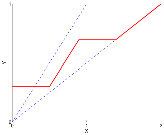
Figure 1: Geometry of basic superposition via a straight line (dashed) in linear spaces versus the polygonal line (solid line) in complete weighted lattices - the polygonal spaces. The polygonal line is $y=\min[\max(x-0.2,0.3),\max(x/2,0.7)]$.

Contributions of our work:
(i) Unify all types of max-$\star$ and min-$\star^{\prime}$ systems under a common theoretical framework of complete weighted lattices (CWLs). Further, while previous work focused mainly on the $(\max,+)$ or $(\min,+)$ formalism, we join both using CWLs and generalize them by replacing $+$ with any operation $\star$ that distributes over $\vee$ and a dual operation $\star^{\prime}$ that distributes over $\wedge$. The corresponding generalized scalar arithmetic is governed by a rich algebraic structure, called clodum, which we developed in previous work [Mara05a, Mara13] and further refine herein. This clodum serves as the ‘field of scalars’ for the CWLs and binds together a pair of dual ‘additions’ with a pair of dual ‘multiplications’; as opposed to max-plus, in some cases the ‘multiplications’ do not have inverses. Two examples different from max-plus, which we analyze in some detail with applications, are the max-product and the max-min cases.

(ii) Analyze the nonlinear system dynamics both in state space using a CWL matrix-vector algebra as well as in the input-output signal space using sup/inf-$\star$ convolutions, represented via lattice monotone operators in adjunction pairs. For the above, we have used the common formalism of CWLs to model both finite- and infinite-dimensional spaces.

(iii) Enable and simplify the analysis and proofs of various results in system representation using lattice adjunctions. Further, use the latter to generate lattice projections that provide optimal solutions for max-$\star$ equations $\boldsymbol{A}\ \framebox(0.0,0.0)[bl]{\star}\ \boldsymbol{x}=\boldsymbol{b}.$ Since the constituent operators of the lattice adjunctions are dilations and erosions which have a geometrical interpretation and have found numerous applications in image analysis, the above perspective to nonlinear system analysis also offers some geometrical insights.

(iv) Study causality, stability, and controllability of max-$\star$ and min-$\star^{\prime}$ systems and link stability with spectral analysis in max-$\star$ algebra and controllability with lattice projections.

(v) Advance the study of special cases employed in many application areas: a) Nonlinear systems represented by max/min-sum ($\star=+$) difference equations, as applied to geometric filtering and shortest path computation. State equations and stability analysis of recursive nonlinear filters. b) Max-product systems ($\star=\times$) that extend the Viterbi algorithm of hidden Markov models to cases with control inputs and can model cognitive processes related to audio-visual attention. c) Probabilistic automata and fuzzy Markov chains governed by max/min rules and with arithmetic based on triangular norms.

Notation:  We think that the currently used notation in max-plus algebra of $\oplus$ and $\otimes$ to denote the maximum $\vee$ (‘addition’) and the $\star$ (‘multiplication’) respectively obscures the lattice operations; in contrast our proposed notation is simpler and more realistic since it uses the well-established symbols $\vee,\wedge$ for sup/inf operations and does not bias the arbitrary scalar binary operation $\star$ with the symbol $\otimes$. Further, the symbol $\oplus$ has been extensively used in signal and image processing for the max-plus signal convolution; herein, we continue this notation. Table 1 summarizes the main symbols of our notation. We use roman letters for functions, signals and their arguments and greek letters for operators. Also, boldface roman letters for vectors (lowcase) and matrices (capital). If $\boldsymbol{M}=[m_{ij}]$ is a matrix, its $(i,j)$th element is also denoted as $\{\boldsymbol{M}\}_{ij}=m_{ij}.$ Similarly, $\boldsymbol{x}=[x_{i}]$ denotes a column vector, whose $i$-th element is denoted as $\{\boldsymbol{x}\}_{i}$ or simply $x_{i}$.

Table 1: Notation for the main algebraic operations

Operation Meaning $\bigvee$ Maximum/Supremum: applies for scalars, vectors and matrices $\bigwedge$ Minimum/Infimum: applies for scalars, vectors and matrices $\ \framebox(0.0,0.0)[bl]{\star}\ \ (\ \framebox(0.0,0.0)[bl]{\star}\,^{\prime}\ )$ General max-$\star$ (min-$\star^{\prime}$) matrix multiplication $\boxplus\ (\boxplus^{\prime})$ Max-sum (min-sum) matrix multiplication $\boxtimes\ (\boxtimes^{\prime})$ Max-product (min-product) matrix multiplication $\hbox{$\,\bigcirc\,$\kern-8.99994pt\hbox{$\star$}$\;\,$}\ (\hbox{$\,\bigcirc\,$\kern-8.99994pt\hbox{$\star$}$\;{}^{\prime}\,$})$ General max-$\star$ (min-$\star^{\prime}$) signal convolution $\oplus\ (\oplus^{\prime})$ Max-sum (min-sum) signal convolution $\otimes\ (\otimes^{\prime})$ Max-product (min-product) signal convolution

2 Lattices and Monotone Operators

Most of the background material in this section follows [Birk67], [Heij94], [HeRo90], [Mara13], and [Serr88].

2.1 Lattices

A partially-ordered set, briefly poset $(\mathcal{P},\leq)$, is a set $\mathcal{P}$ with a binary relation $\leq$ that is a partial ordering, i.e. is reflexive, antisymmetric and transitive. If, in addition, for any two elements $X,Y\in\mathcal{P}$ we have either $X\leq Y$ or $Y\leq X$, then $\mathcal{P}$ is called a chain. To every partial ordering $\leq$ there corresponds a dual partial ordering $\leq^{\prime}$ defined by “$X\leq^{\prime}Y$ iff $X\geq Y$”. Let $\mathcal{S}$ be a subset of $(\mathcal{P},\leq)$; an upper bound of $\mathcal{S}$ is an element $B\in\mathcal{P}$ such that $X\leq B$ for all $X\in\mathcal{S}$. The least upper bound of $\mathcal{S}$ is called its supremum and denoted by $\sup\mathcal{S}$ or $\bigvee\mathcal{S}$. By duality, we define the greatest lower bound of $\mathcal{S}$, called its infimum and denoted by $\inf\mathcal{S}$ or $\bigwedge\mathcal{S}$. If the supremum (resp. infimum) of $\mathcal{S}$ belongs to $\mathcal{S}$, then it is called the greatest element or maximum (resp. least element or minimum) of $\mathcal{S}$. An element $M$ of $\mathcal{S}$ is called maximal (resp. minimal) if there is no other element in $\mathcal{S}$ that is greater (resp. smaller) than $M$.

A lattice is a poset $(\mathcal{L},\leq)$ any two of whose elements have a supremum, denoted by $X\vee Y$, and an infimum, denoted by $X\wedge Y$. We often denote the lattice structure by $(\mathcal{L},\vee,\wedge)$. A lattice $\mathcal{L}$ is complete if each of its subsets (finite or infinite) has a supremum and an infimum in $\mathcal{L}$. Any nonempty complete lattice is universally bounded because it contains its supremum $\top=\bigvee\mathcal{L}$ and infimum $\bot=\bigwedge\mathcal{L}$ which are its greatest (top) and least (bottom) elements, respectively. In any lattice $\mathcal{L}$, by replacing the partial ordering with its dual and by interchanging the roles of the supremum and infimum we obtain a dual lattice $\mathcal{L}^{\prime}$. Duality principle: to every definition, property and statement that applies to $\mathcal{L}$ there corresponds a dual one that applies to $\mathcal{L}^{\prime}$ by interchanging $\leq$ with $\leq^{\prime}$ and $\vee$ with $\wedge$. A bijection between two lattices $\mathcal{L}$ and $\mathcal{M}$ is called an isomorphism (resp. dual isomorphism) if it preserves (resp. reverses) suprema and infima. If $\mathcal{L}=\mathcal{M}$, a (dual-) isomorphism on $\mathcal{L}$ is called (dual-) automorphism.

The lattice operations satisfy many properties, as summarized in Table 3. Conversely, a set $\mathcal{L}$ equipped with two binary operations $\vee$ and $\wedge$ that satisfy properties (L1,L1${}^{\prime}$)–(L5,L5${}^{\prime}$) is a lattice whose supremum is $\vee$, the infimum is $\wedge$, and partial ordering $\leq$ is given by (L6). A lattice $(\mathcal{L},\vee,\wedge)$ contains two weaker substructures: a sup-semilattice $(\mathcal{L},\vee)$ that satisfies properties (L$1-$L4) and an inf-semilattice $(\mathcal{L},\wedge)$ that satisfies properties (L1${}^{\prime}-$L4${}^{\prime}$).

The additional properties (L7,L7${}^{\prime}$) and (L8,L8${}^{\prime}$) in Table 3 hold only if the lattice contains a least and a greatest element, respectively. A lattice $\mathcal{L}$ is called distributive if it satisfies properties (L9,L9${}^{\prime}$); if these also hold over infinite set collections, then the lattice is called infinitely distributive. The rest of the properties of Table 3, labeled as “WL#”, refer to a richer algebra defined as ‘weighted lattices’ in Section 3.2.

Examples 1

(a) Any chain is an infinitely distributive lattice. Thus, the chain $(\mathbb{R},\leq)$ of real numbers equipped with the natural order $\leq$ is a lattice, but not complete. The set of extended real numbers $\overline{\mathbb{R}}=\mathbb{R}\cup\{-\infty,+\infty\}$ is a complete lattice.

(b) The power set $\mathcal{P}(E)=\{X:X\subseteq\,E\}$ of an arbitrary set $E$ equipped with the partial order of set inclusion is an infinitely distributive lattice under the supremum and infimum induced by set inclusion which are the set union and intersection, respectively.

(c) In a lattice $\mathcal{L}$ with universal bounds $\bot$ and $\top$, an element $X\in\mathcal{L}$ is said to have a complement $X^{c}\in\mathcal{L}$ if $X\vee X^{c}=\top$ and $X\wedge X^{c}=\bot$. If all the elements of $\mathcal{L}$ have complements, then $\mathcal{L}$ is called complemented. Any complemented and distributive lattice $\mathcal{B}$ is called a Boolean lattice.

(d) Let $\mathcal{L}^{E}=\mathrm{Fun}(E,\mathcal{L})$ denote the set of all functions $f:E\rightarrow\mathcal{L}$. If $\leq$ is the partial ordering of $\mathcal{L}$, we can equip the function space $\mathcal{L}^{E}$ with the pointwise partial ordering $f\leq g$, which means $f(x)\leq g(x)\;\forall x\in E$, the pointwise supremum $(\bigvee_{i}f_{i})(x)=\bigvee_{i}f_{i}(x)$, and pointwise infimum $(\bigwedge_{i}f_{i})(x)=\bigwedge_{i}f_{i}(x)$. Then, $(\mathcal{L}^{E},\vee,\wedge)$ becomes a function lattice, which retains possible properties of $\mathcal{L}$ of being complete, or (infinitely) distributive, or Boolean.

2.2 Operators on Lattices

Let $\mathcal{O}(\mathcal{L})$ be the set of all operators on a complete lattice $\mathcal{L}$, i.e., mappings from $\mathcal{L}$ to itself. Given two such operators $\psi$ and $\phi$ we can define a partial ordering between them ($\phi\leq\psi$), their supremum ($\psi\vee\phi$) and infimum ($\psi\wedge\phi$) in a pointwise way, as done in Example 1(d). This makes $\mathcal{O}(\mathcal{L})$ a complete function lattice which inherits many of the possible properties of $\mathcal{L}$. Further, we define the composition of two operators as an operator product: $\psi\phi(X)\,\triangleq\,\psi(\phi(X))$; special cases are the operator powers $\psi^{n}=\psi\psi^{n-1}$. Some useful types and properties of lattice operators $\psi$ include the following: (i) identity: $\mathbf{id}(X)=X$ $\;\forall X\in\mathcal{L}$. (ii) extensive: $\psi\geq\mathbf{id}$. (iii) antiextensive: $\psi\leq\mathbf{id}$. (iv) idempotent: $\psi^{2}=\psi$. (v) involution: $\psi^{2}=\mathbf{id}$.

2.2.1 Monotone Operators

Of great interest are the monotone operators, whose collections form sublattices of $\mathcal{O}(\mathcal{L})$. They come in three basic kinds according to which of the following lattice structures they preserve (or map to its dual): (i) partial ordering, (ii) supremum, (iii) infimum.

A lattice operator $\psi$ is called increasing or isotone if it is order-preserving, i.e. $X\leq Y\Longrightarrow\psi(X)\leq\psi(Y)$. A lattice operator $\psi$ is called decreasing or antitone if it is order-inverting, i.e. $X\leq Y\Longrightarrow\psi(X)\geq\psi(Y)$.

Examples of increasing operators are the lattice homomorphisms which preserve suprema and infima over finite collections. If a lattice homomorphism is also a bijection, then it becomes an automorphism. A bijection $\phi$ is an automorphism if both $\phi$ and its inverse $\phi^{-1}$ are increasing.

Four types of increasing operators, fundamental for unifying systems on lattices, are the following:

$$\begin{array}[]{rcl}\mbox{\mbox{\large$\delta$}\ is {dilation}}&\mathrm{iff}&\mbox{\large$\delta$}(\bigvee_{i\in J}X_{i})=\bigvee_{i\in J}\mbox{\large$\delta$}(X_{i})\\ \mbox{\mbox{\large$\varepsilon$}\ is {erosion}}&\mathrm{iff}&\mbox{\large$\varepsilon$}(\bigwedge_{i\in J}X_{i})=\bigwedge_{i\in J}\mbox{\large$\varepsilon$}(X_{i})\\ \mbox{\mbox{\large$\alpha$}\ is {opening}}&\mathrm{iff}&\mbox{increasing, idempotent, antiextensive}\\ \mbox{\mbox{\large$\beta$}\ is {closing}}&\mathrm{iff}&\mbox{increasing, idempotent, extensive}\end{array}$$

Dilations and erosions require arbitrary (possibly infinite) collections $\{X_{i}:i\in J\}$ of lattice elements; hence, they need complete lattices. The special case of an empty collection equips each dilation and erosion with the following necessary properties:

$$\mbox{\large$\delta$}(\bot)=\bot,\quad\mbox{\large$\varepsilon$}(\top)=\top$$ (12)

The four above types of lattice operators were originally defined in [Serr88, Heij94] as generalizations of the corresponding Minkowski-type morphological operators and have been applied in numerous image processing tasks.

Examples of decreasing operators are the dual homomorphisms, which interchange suprema with infima. A lattice dual-automorphism is a bijection $\theta$ that interchanges suprema with infima, or equivalently iff it is a bijection and both $\theta$ and its inverse $\theta^{-1}$ are decreasing. A negation $\nu$ is a dual automorphism that is also involutive; we may write $X^{\neg}=\nu(X)$ for the negative of a lattice element. Given an operator $\psi$ in a lattice equipped with a negation, its corresponding negative (a.k.a. dual) operator is defined as $\psi^{\neg}(X)\,\triangleq\,[\psi(X^{\neg})]^{\neg}$. For example, the most well-known negation on the set lattice $\mathcal{P}(E)$ is the complementation $\nu(X)=X^{c}=E\setminus X$, whereas on the function lattice $\mathrm{Fun}(E,\overline{\mathbb{R}})$ the most well-known negation is $\nu(f)=-f$.

The above definitions allow broad classes of operators on vector or signal spaces to be grouped as parallel or sequential combinations of lattice monotone operators and their common properties to be studied under the unifying lattice framework. In this work we shall find them very useful for representing the state and output responses or for approximating solutions of systems obeying a supremal or infimal superposition.

2.2.2 Order Continuity

Consider an arbitrary sequence $(X_{n})$ of elements in a complete lattice $\mathcal{L}$. The following two limits can be defined using only sup/inf combinations:

$$\limsup X_{n}\,\triangleq\,\bigwedge_{n\geq 1}\bigvee_{k\geq n}X_{k}\;\;,\;\;\liminf X_{n}\,\triangleq\,\bigvee_{n\geq 1}\bigwedge_{k\geq n}X_{k}$$ (13)

In general, $\liminf X_{n}\leq\limsup X_{n}$. A sequence $(X_{n})$ is defined to order converge to a lattice element $X$, written as $X_{n}\,\stackrel{{\scriptstyle\mathrm{ord}}}{{\rightarrow}}\,X$, if $\liminf X_{n}=\limsup X_{n}=X$.

An operator $\psi$ on $\mathcal{L}$ is called $\downarrow$-continuous if $(X_{n})\,\stackrel{{\scriptstyle\mathrm{ord}}}{{\rightarrow}}\,X$ in $\mathcal{L}$ implies that $\limsup\psi(X_{n})\leq\psi(X)$. Dually, $\psi$ is called $\uparrow$-continuous if $(X_{n})\,\stackrel{{\scriptstyle\mathrm{ord}}}{{\rightarrow}}\,X$ implies that $\liminf\psi(X_{n})\geq\psi(X)$. Finally, $\psi$ is called order continuous if it is both $\downarrow$-continuous and $\uparrow$-continuous. On a chain, e.g. $(\overline{\mathbb{R}},\leq)$, the concepts of order convergence and order continuity coincide with their topological counterparts.

There is a stronger form of order convergence applicable to monotone sequences [Heij94]. We write $X_{n}\downarrow X$ to mean a monotonic convergence where $(X_{n})$ is a decreasing sequence ($X_{n+1}\leq X_{n}$) and $X=\bigwedge_{n}X_{n}$. Dually, we write $X_{n}\uparrow X$ to mean that $(X_{n})$ is an increasing sequence ($X_{n+1}\geq X_{n}$) and $X=\bigvee_{n}X_{n}$. This monotonic convergence allows to easily examine the order continuity of increasing operators. Specifically, an increasing operator $\psi$ on a complete lattice $\mathcal{L}$ is $\downarrow$-continuous iff $X_{n}\downarrow X$ implies that $\psi(X_{n})\downarrow\psi(X)$ for any sequence $(X_{n})$. Dually, $\psi$ is $\uparrow$-continuous iff $X_{n}\uparrow X$ implies that $\psi(X_{n})\uparrow\psi(X)$. This result implies that, since dilations (resp. erosions) distribute over arbitrary suprema (resp. infima), dilations are $\uparrow$-continuous, whereas erosions are $\downarrow$-continuous.

2.2.3 Residuation and Adjunctions

An increasing operator $\psi$ on a complete lattice $\mathcal{L}$ is called residuated [Blyt05, BlJa72] if there exists an increasing operator ${\psi}^{\sharp}$ such that

$$\psi{\psi}^{\sharp}\leq\mathbf{id}\leq{\psi}^{\sharp}\psi$$ (14)

${\psi}^{\sharp}$ is called the residual of $\psi$ and is the closest to being an inverse of $\psi$. Specifically, the residuation pair ($\psi,{\psi}^{\sharp})$ can solve inverse problems of the type $\psi(X)=Y$ either exactly since $\hat{X}={\psi}^{\sharp}(Y)$ is the greatest solution of $\psi(X)=Y$ if a solution exists, or approximately since $\hat{X}$ is the greatest subsolution in the sense that $\hat{X}=\bigvee\{X:\psi(X)\leq Y\}$. On complete lattices an increasing operator $\psi$ is residuated (resp. a residual ${\psi}^{\sharp}$) if and only if it is a dilation (resp. erosion). The residuation theory has been used for solving inverse problems in matrix algebra [Cuni79, BCOQ01, CGQ04] over the max-plus or other idempotent semirings.

Dilations and erosions come in pairs as the following concept reveals. The pair $(\mbox{\large$\delta$},\mbox{\large$\varepsilon$})$ of operators on a complete lattice $\mathcal{L}$ is called an adjunction on $\mathcal{L}$ if

$$\mbox{\large$\delta$}(X)\leq Y\Longleftrightarrow X\leq\mbox{\large$\varepsilon$}(Y)\quad\forall X,Y\in\mathcal{L}$$ (15)

In any adjunction, (15) implies that $\delta$ is a dilation and $\varepsilon$ is an erosion. It can be shown that this double inequality is equivalent to the inequality (14) satisfied by a residuation pair of increasing operators if we identify the residuated map $\psi$ with $\delta$ and its residual ${\psi}^{\sharp}$ with $\varepsilon$. To view $(\mbox{\large$\delta$},\mbox{\large$\varepsilon$})$ as an adjunction instead of a residuation pair has the advantage of the additional geometrical intuition and visualization afforded by the dilation and erosion operators, which are well-known in image analysis and can be interpreted as augmentation and shrinkage respectively of input sets or of hypographs of functions.

In any adjunction $(\mbox{\large$\delta$},\mbox{\large$\varepsilon$})$, $\varepsilon$ is called the adjoint erosion of $\delta$, whereas $\delta$ is the adjoint dilation of $\varepsilon$. There is a one-to-one correspondence between the two operators of an adjunction pair, since, given a dilation $\delta$, there is a unique erosion

$$\mbox{\large$\varepsilon$}(Y)=\bigvee\{X\in\mathcal{L}:\mbox{\large$\delta$}(X)\leq Y\}$$ (16)

such that $(\mbox{\large$\delta$},\mbox{\large$\varepsilon$})$ is adjunction. Conversely, given an erosion $\varepsilon$, there is a unique dilation

$$\mbox{\large$\delta$}(X)=\bigwedge\{Y\in\mathcal{L}:\mbox{\large$\varepsilon$}(Y)\geq X\}$$ (17)

such that $(\mbox{\large$\delta$},\mbox{\large$\varepsilon$})$ is adjunction. Adjunctions create operator duality pairs that are different than negation in the sense that one operator is the closest to being the inverse of the other, either from below or above.

2.2.4 Projections on Lattices

A large variety of useful lattice operators share two properties: increasing and idempotent. Such operators were called morphological filters in [Heij94, Serr88]. We shall call them lattice projections of the order type, since they preserve the lattice ordering and are idempotent in analogy with the linear projections that preserve the algebraic structure of linear spaces and are idempotent. Two well-studied special cases of lattice projections are the openings and closings, each of which has an additional property. Specifically, openings are lattice projections that are anti-extensive, whereas closings are extensive projections. Combinations of such generalized filters have proven to be very useful for signal denoising, image enhancement, simplification, segmentation, and object detection. From the composition of the erosion and dilation of any adjunction $(\mbox{\large$\delta$},\mbox{\large$\varepsilon$})$ we can generate a projection $\mbox{\large$\alpha$}=\mbox{\large$\delta$}\mbox{\large$\varepsilon$}$ that is also an opening since $\mbox{\large$\alpha$}(X)\leq X$ and $\mbox{\large$\alpha$}^{2}=\mbox{\large$\alpha$}$. To prove this note that, by (15),

$$\mbox{\large$\delta$}\mbox{\large$\varepsilon$}\leq\mathbf{id}\leq\mbox{\large$\varepsilon$}\mbox{\large$\delta$}$$ (18)

which implies that $\mbox{\large$\delta$}\mbox{\large$\varepsilon$}\mbox{\large$\delta$}\mbox{\large$\varepsilon$}=\mbox{\large$\delta$}\mbox{\large$\varepsilon$}$. Dually, any adjunction can also generate a closing projection $\mbox{\large$\beta$}=\mbox{\large$\varepsilon$}\mbox{\large$\delta$}$, which always satisfies $\mbox{\large$\beta$}(X)\geq X$ and $\mbox{\large$\beta$}^{2}=\mbox{\large$\beta$}$. There are also other types of lattice projections that are studied in [CGQ04].

2.3 Lattice-Ordered Monoids and Clodum

A lattice $(\mathcal{M},\vee,\wedge)$ is often endowed with a third binary operation, called symbolically the ‘multiplication’ $\star$, under which $(\mathcal{M},\star)$ is a group or monoid or just semigroup [Birk67].

Consider now an algebra $(\mathcal{M},\vee,\wedge,\star,\star^{\prime})$ with four binary operations, which we call a lattice-ordered double monoid, where $(\mathcal{M},\vee,\wedge)$ is a lattice, $(\mathcal{M},\star)$ is a monoid whose ‘multiplication’ $\star$ distributes over $\vee$, and $(\mathcal{M},\star^{\prime})$ is a monoid whose ‘multiplication’ $\star^{\prime}$ distributes over $\wedge$. These distributivities imply that both $\star$ and $\star^{\prime}$ are increasing. To the above definitions we add the word complete if $\mathcal{M}$ is a complete lattice and the distributivities involved are infinite. We call the resulting algebra a complete lattice-ordered double monoid, in short clodum [Mara05a, Mara13].

Previous works on minimax or max-plus algebra and their applications have used alternative names for algebraic structures similar to the above definitions which emphasize semigroups and semirings instead of lattices. If $\star=\star^{\prime}$, we have a self-dual ‘multiplication’. This always happens if $(\mathcal{M},\star)$ is a group, i.e. a monoid where each element has an inverse; in this case we obtain a lattice-ordered group, and the group ‘multiplication’ $X\mapsto A\star X$ is a lattice automorphism.

We give a precise definition of a general clodum and some examples since this will be one of the fundamental algebraic structures to build the nonlinear spaces in our work. An algebraic structure $(\mathcal{K},\vee,\wedge,\star,\star^{\prime})$ is called a clodum if:
(C1) $(\mathcal{K},\vee,\wedge)$ is a complete distributive lattice.
(C2) $(\mathcal{K},\star)$ is a monoid whose operation $\star$ is a dilation.
(C3) $(\mathcal{K},\star^{\prime})$ is a monoid whose operation $\star^{\prime}$ is an erosion.

Remarks: (i) As a lattice, $\mathcal{K}$ is not necessarily infinitely distributive, although in this paper all our examples will be such.
(ii) The clodum ‘multiplications’ $\star$ and $\star^{\prime}$ do not have to be commutative.
(iii) The least (greatest) element $\bot$ ($\top$) of $\mathcal{K}$ is both the identity element for $\vee$ ($\wedge$) and an absorbing null for $\star$ ($\star^{\prime}$) due to (12).

If $\star=\star^{\prime}$ over $G=\mathcal{K}\setminus\{\bot,\top\}$ where $(G,\star)$ is a group and $(G,\vee,\wedge)$ a conditionally complete lattice, then the clodum $\mathcal{K}$ becomes a richer structure which we call a complete lattice-ordered group, in short clog. By extending properties of lattice-ordered groups [Birk67] to clogs, we can show that in any clog the distributivity between $\vee$ and $\wedge$ is of the infinite type and the ‘multiplications’ $\star$ and $\star^{\prime}$ are commutative. Thus, a clog has a richer structure than a blog (bounded lattice-ordered group) as defined in [Cuni79], because a clog is a complete and commutative blog.

Examples 2

(a) Our scalar arithmetic in this paper will use a numeric commutative clodum. Two such examples follow:
(a1) Max-plus clog:  $(\overline{\mathbb{R}},\vee,\wedge,+,+^{\prime})$, where $\vee/\wedge$ denote the standard sup/inf on $\overline{\mathbb{R}}$, $+$ is the standard addition on the set $\overline{\mathbb{R}}$ of extended reals playing the role of a ‘multiplication’ $\star$ with $+^{\prime}$ being the ‘dual multiplication’ $\star^{\prime}$; the operations $+$ and $+^{\prime}$ are identical for finite reals, but $a+(-\infty)=-\infty$ and $a+^{\prime}(+\infty)=+\infty$ for all $a\in\overline{\mathbb{R}}$.
(a2) Max-min clodum:  $([0,1],\vee,\wedge,\min,\max)$, where $\star=\min$ and $\star^{\prime}=\max$.
(b) Matrix max-sum clodum: $(\overline{\mathbb{R}}^{n\times n},\vee,\wedge,\boxplus,\boxplus^{\prime})$ where $\overline{\mathbb{R}}^{n\times n}$ is the set of $n\times n$ matrices with entries from $\overline{\mathbb{R}}$, $\vee$ and $\wedge$ denote here element-wise matrix supremum and infimum, and $\boxplus,\boxplus^{\prime}$ denote max-sum and min-sum matrix ‘multiplications’:

$$\boldsymbol{C}=\boldsymbol{A}\boxplus\boldsymbol{B}=[c_{ij}] \;c_{ij}={\displaystyle\bigvee_{k=1}^{n}}a_{ik}+b_{kj}$$ , (19)

$$\boldsymbol{C}=\boldsymbol{A}\boxplus^{\prime}\boldsymbol{B}=[c_{ij}] \;c_{ij}={\displaystyle\bigwedge_{k=1}^{n}}a_{ik}+^{\prime}b_{kj}$$ , (20)

This is a clodum with non-commutative ‘multiplications’.

3 Representations of Vector and Signal Operations on Weighted Lattices

3.1 Algebraic Structures on the Scalars

We assume that all elements of the vectors, matrices, or signals involved in the description of the systems examined herein take their values from a set $\mathcal{K}$ of scalars, which in general will be a subset of $\overline{\mathbb{R}}=\mathbb{R}\cup\{-\infty,\infty\}$ with the natural ordering $\leq$ of extended real numbers. We assume that the chain $(\mathcal{K},\leq)$ is universally bounded, i.e., contains its least $\bot\,\triangleq\,\bigwedge\mathcal{K}$ and greatest element $\top\,\triangleq\,\bigvee\mathcal{K}$. For the weighted lattice model we need to equip $\mathcal{K}$ with four binary operations:

(A). The standard maximum or supremum $\vee$ on $\overline{\mathbb{R}}$, which plays the role of a generalized ‘addition’.

(A${}^{\prime}$). The standard minimum or infimum $\wedge$ on $\overline{\mathbb{R}}$, which plays the role of a generalized ‘dual addition’.

(M). A commutative generalized ‘multiplication’ $\star$ under which: (i) $\mathcal{K}$ is a monoid with (‘unit’) identity element $e$ and (‘zero’) null element $\bot$, i.e.,

$$a\star e=a,\quad a\star\bot=\bot,\quad\forall a\in\mathcal{K},$$ (21)

and (ii) $\star$ is a scalar dilation, i.e., distributes over any supremum:

$$a\star(\bigvee_{i}x_{i})=\bigvee_{i}a\star x_{i}$$ (22)

(M${}^{\prime}$). A commutative ‘dual  multiplication’ $\star^{\prime}$ under which: (i) $\mathcal{K}$ is a monoid with identity $e^{\prime}$ and null element $\top$, i.e.,

$$a\star^{\prime}e^{\prime}=a,\quad a\star^{\prime}\top=\top,\quad\forall a\in\mathcal{K},$$ (23)

and (ii) $\star^{\prime}$ is a scalar erosion, i.e., distributes over any infimum:

$$a\star^{\prime}(\bigwedge_{i}x_{i})=\bigwedge_{i}a\star^{\prime}x_{i}$$ (24)

Under the above assumptions $(\mathcal{K},\vee,\wedge,\star,\star^{\prime})$ becomes a scalar clodum. Note that, in addition to the minimal requirements of a general clodum in Sec. 2.3, we assume commutative operations $\star,\star^{\prime}$. Further, the rich structure of $\overline{\mathbb{R}}$ endows the set $\mathcal{K}$ to be infinitely distributive as a lattice. This will be the most general and minimally required algebraic structure we consider for the set of scalars. We avoid degenerate cases by assuming that $\vee\not=\star$ and $\wedge\not=\star^{\prime}$. However, $\star$ may be the same as $\star^{\prime}$, in which case we have a self-dual ‘multiplication’.

A clodum $\mathcal{K}$ is called self-conjugate if it has a lattice negation (i.e. involutive dual automorphism) that maps each element $a$ to its conjugate ${a}^{\ast}$ such that

$${(\bigvee_{i}a_{i})}^{\ast}=\bigwedge_{i}{a_{i}}^{\ast}\;\;,\;\;{(\bigwedge_{i}b_{i})}^{\ast}=\bigvee_{i}{b_{i}}^{\ast}\;\;,\;\;{(a\star b)}^{\ast}={a}^{\ast}\star^{\prime}{b}^{\ast}$$ (25)

We assume that the suprema and infima in (25) may be over any (possibly infinite) collections.

The set of scalars can be partitioned as $\mathcal{K}=G\cup\{\bot,\top\}$; the members of $G$ are called the finite scalars, borrowing terminology from the case when $\mathcal{K}=\overline{\mathbb{R}}$. This is useful for cases where $(G,\star)$ is a commutative group. Then, for each $a\in G$ there exists its ‘multiplicative inverse’ $a^{-1}$ such that $a\star a^{-1}=e$. Further, the ‘multiplication’ $\star$ and its self-dual $\star^{\prime}$ (which coincide over $G$) can be extended over the whole $\mathcal{K}$ by adding the rules in (21) and (23) involving the null elements. As defined in Sec. 2.3, the resulting richer structure is a clog. Whenever $\mathcal{K}$ is a clog, it becomes self-conjugate by setting

$${a}^{\ast}=\left\{\begin{array}[]{lll}a^{-1}&\mathrm{if}&\bot<a<\top\\ \top&\mathrm{if}&a=\bot\\ \bot&\mathrm{if}&a=\top\end{array}\right.$$ (26)

Next we further elaborate on three main examples used in this paper for a scalar clodum.

Examples 3

(a) Max-plus clog  $(\overline{\mathbb{R}},\vee,\wedge,+,+^{\prime})$: This is the archetypal example of a clog. The identities are $e=e^{\prime}=0$, the nulls are $\bot=-\infty$ and $\top=+\infty$, and the conjugation mapping is ${a}^{\ast}=-a$.
(b) Max-times clog $([0,+\infty],\vee,\wedge,\times,\times^{\prime})$: The identities are $e=e^{\prime}=1$, the nulls are $\bot=0$ and $\top=+\infty$, and the conjugation mapping is ${a}^{\ast}=1/a$.
(c) Max-min clodum  $([0,1],\vee,\wedge,\min,\max)$: As ‘multiplications’ we have $\star=\min$ and $\star^{\prime}=\max$. The identities and nulls are $e^{\prime}=\bot=0$, $e=\top=1$. A possible conjugation mapping is ${a}^{\ast}=1-a$. Additional cloda that are not clogs are discussed in Sec. 9.3 using more general fuzzy intersections and unions.

Table 2: Scalar Arithmetic in a CLOG

$a\in\mathcal{K}$ $b\in\mathcal{K}$ $\vee$ $\wedge$ $\star$ $\star^{\prime}$ $\bot$ $\bot$ $\bot$ $\bot$ $\bot$ $\bot$ $\bot$ $y\in G$ $y$ $\bot$ $\bot$ $\bot$ $\bot$ $\top$ $\top$ $\bot$ $\bot$ $\top$ $x\in G$ $y\in G$ $x\vee y$ $x\wedge y$ $x\star y$ $x\star^{\prime}y$ $\top$ $\bot$ $\top$ $\bot$ $\bot$ $\top$ $\top$ $y\in G$ $\top$ $y$ $\top$ $\top$ $\top$ $\top$ $\top$ $\top$ $\top$ $\top$

Table 2 summarizes the results of all scalar binary operations in a clog. We see that in a clog the $\star$ and $\star^{\prime}$ coincide in all cases with only one exception: the combination of the least and greatest elements. Henceforth when a clodum $\mathcal{K}$ is a clog we can denote the algebra as $(\mathcal{K},\vee,\wedge,\star)$ using only one ‘multiplication’ operation and the case $\bot\star\top$ will have value $\bot$ (resp. $\top$) if it is combined with other terms via a supremum (resp. infimum).

3.2 Complete Weighted Lattices

Consider a nonempty collection $\mathcal{W}$ of mathematical objects, which will be our space; examples of such objects include the vectors in $\overline{\mathbb{R}}^{n}$ or signals in $\mathrm{Fun}(E,\overline{\mathbb{R}})$. Thus, we shall symbolically refer to the space elements as ‘vectors/signals’, although they may be arbitrary objects. Also, consider a clodum $(\mathcal{K},\vee,\wedge,\star,\star^{\prime})$ of ‘scalars’. We define two internal operations among vectors/signals $X,Y$ in $\mathcal{W}$: their supremum $X\vee Y:\mathcal{W}^{2}\rightarrow\mathcal{W}$ and infimum $X\wedge Y:\mathcal{W}^{2}\rightarrow\mathcal{W}$, which we denote using the same supremum symbol ($\vee$) and infimum symbol ($\wedge$) as in the clodum, hoping that the differences will be clear to the reader from the context. Further, we define two external operations among any vector/signal $X$ in $\mathcal{W}$ and any scalar $c$ in $\mathcal{K}$: a ‘scalar multiplication’ $c\star X:(\mathcal{K},\mathcal{W})\rightarrow\mathcal{W}$ and a ‘scalar dual multiplication’ $c\star^{\prime}X:(\mathcal{K},\mathcal{W})\rightarrow\mathcal{W}$, again by using the same symbols as in the clodum. Now, we define $\mathcal{W}$ to be a weighted lattice space over the clodum $\mathcal{K}$ if for all $X,Y,Z\in\mathcal{W}$ and $a,b\in\mathcal{K}$ all the axioms of Table 3 hold. Note that: (a) Under axioms L1-L9 and their duals L1${}^{\prime}$-L9${}^{\prime}$, $\mathcal{W}$ is a distributive lattice with a least element ($O$) and a greatest element ($I$). (b) These axioms bear a striking similarity with those of a linear space. One difference is that the vector/signal addition ($+$) of linear spaces is now replaced by two dual superpositions, the lattice supremum ($\vee$) and infimum ($\wedge$); further, the scalar multiplication ($\times$) of linear spaces is now replaced by two operations $\star$ and $\star^{\prime}$ that are dual to each other. Only one major property of the linear spaces is missing from the weighted lattices: the existence of ‘additive inverses’; i.e., the supremum and infimum operations do not have inverses.

Table 3: Axioms of Weighted Lattices

Sup-Semilattice	Inf-Semilattice	Description
L1. $\;X\vee Y\in\mathcal{W}$	L1${}^{\prime}.\;X\wedge Y\in\mathcal{W}$	Closure of $\vee,\wedge$
L2. $\;X\vee X=X$	L2${}^{\prime}.\;X\wedge X=X$	Idempotence of $\vee,\wedge$
L3. $\;X\vee Y=Y\vee X$	L3${}^{\prime}.\;X\wedge Y=Y\wedge X$	Commutativity of $\vee,\wedge$
L4. $\;X\vee(Y\vee Z)=$	L4${}^{\prime}.\;X\wedge(Y\wedge Z)=$	Associativity of $\vee,\wedge$
$(X\vee Y)\vee Z$	$(X\wedge Y)\wedge Z$
L5. $\;X\vee(X\wedge Y)=X$	L5${}^{\prime}.\;X\wedge(X\vee Y)=X$	Absorption between $\vee,\wedge$
L6. $\;X\leq Y\Longleftrightarrow$	L6${}^{\prime}.\;X\leq^{\prime}Y\Longleftrightarrow$	Consistency of $\vee,\wedge$
$Y=X\vee Y$	$Y=X\wedge Y$	with partial order $\leq$
L7. $\;O\vee X=X$	L7${}^{\prime}.\;I\wedge X=X$	Identities of $\vee,\wedge$
L8. $\;I\vee X=I$	L8${}^{\prime}.\;O\wedge X=O$	Absorbing Nulls of $\vee,\wedge$
L9. $\;X\vee(Y\wedge Z)=$	L9${}^{\prime}.\;X\wedge(Y\vee Z)=$	Distributivity of $\vee,\wedge$
$(X\vee Y)\wedge(X\vee Z)$	$(X\wedge Y)\vee(X\wedge Z)$
WL10. $\;a\star X\in\mathcal{W}$	WL10${}^{\prime}.\;a\star^{\prime}X\in\mathcal{W}$	Closure of $\star,\star^{\prime}$
WL11. $\;a\star(b\star X)=$	WL11${}^{\prime}.\;a\star^{\prime}(b\star^{\prime}X)=$	Associativity of $\star,\star^{\prime}$
$(a\star b)\star X$	$(a\star^{\prime}b)\star^{\prime}X$
WL12. $\;a\star(X\vee Y)=$	WL12${}^{\prime}.\;a\star^{\prime}(X\wedge Y)=$	Distributive scalar-vector
$a\star X\vee a\star Y$	$a\star^{\prime}X\wedge a\star^{\prime}Y$	mult over vector sup/inf
WL13. $\;(a\vee b)\star X=$	WL13${}^{\prime}.\;(a\wedge b)\star^{\prime}X=$	Distributive scalar-vector
$a\star X\vee b\star X$	$a\star^{\prime}X\wedge b\star^{\prime}X$	mult over scalar sup/inf
WL14. $\;e\star X=X$	WL14${}^{\prime}.\;e^{\prime}\star^{\prime}X=X$	Scalar Identities
WL15. $\;\bot\star X=O$	WL15${}^{\prime}.\;\top\star^{\prime}X=I$	Scalar Nulls
WL16. $\;a\star O=O$	WL16${}^{\prime}.\;a\star^{\prime}I=I$	Vector Nulls

We define the weighted lattice $\mathcal{W}$ to be a complete weighted lattice (CWL) space if all the following hold:
(i)  $\mathcal{W}$ is closed under any, possibly infinite, suprema and infima.
(ii) The distributivity laws between the scalar operations $\star$ ($\star^{\prime}$) and the supremum (infimum) are of the infinite type.
Note that, a clodum is by itself a complete weighted lattice over itself.

Consider a subset $\mathcal{A}$ of a complete weighted lattice $\mathcal{W}$ over a clodum $\mathcal{K}$. A space element $F$ is called a sup-$\star$ combination of points in $\mathcal{A}$ if there exists an indexed set of space elements $\{F_{i}\}$ in $\mathcal{A}$ and a corresponding set of scalars $\{a_{i}\}$ in $\mathcal{K}$ such that

$$F=\bigvee_{i}a_{i}\star F_{i},$$ (27)

Dually, we can form an inf-$\star^{\prime}$ combination $G=\bigwedge_{i}b_{i}\star^{\prime}G_{i}$ of points $G_{i}$ in $\mathcal{A}$ with scalars $b_{i}$. The sup-$\star$ span of $\mathcal{A}$, denoted by $\mathrm{span}_{\vee}(\mathcal{A})$, is the set of all sup-$\star$ combinations of elements in $\mathcal{A}$. If $\mathcal{A}=\varnothing$, then $\mathrm{span}_{\vee}(\mathcal{A})=\{O\}$. Dually, the set of all inf-$\star^{\prime}$ combinations of elements in $\mathcal{A}$ is called its inf-$\star^{\prime}$ span, denoted by $\mathrm{span}_{\wedge}(\mathcal{A})$. If $\mathcal{A}=\varnothing$, then $\mathrm{span}_{\wedge}(\mathcal{A})=\{I\}$.

If the above sup-$\star$ and inf-$\star^{\prime}$ combinations are based on a finite set of space elements, we shall call them max-$\star$ and min-$\star^{\prime}$ combination, respectively. A set $\mathcal{S}$ in a complete weighted lattice is called max-$\star$ independent if each point $F\in\mathcal{S}$ is not a max-$\star$ combination of points in $\mathcal{S}\setminus\{F\}$; otherwise, the set is called max-$\star$ dependent. Dually for the min-$\star^{\prime}$ (in)dependence.

A max-$\star$ independent subset $\mathcal{B}$ of a CWL $\mathcal{W}$ is called an upper basis for the space if each space element $F$ can be represented as a sup-$\star$ combination of basis elements:

$$F=\bigvee_{i}c_{i}\star B_{i},\;\;B_{i}\in\mathcal{B}$$ (28)

Dually, a min-$\star^{\prime}$ independent subset $\mathcal{B}^{\prime}$ of $\mathcal{W}$ is called a lower basis if $\mathcal{W}=\mathrm{span}_{\wedge}(\mathcal{B}^{\prime})$. Examples of upper and lower bases are given later for CWLs of functions.

In this paper we shall focus on CWLs whose underlying set is a function space $\mathcal{W}=\mathrm{Fun}(E,\mathcal{K})$ where $E$ is an arbitrary nonempty set serving as the domain of our functions and the values of these functions are from a clodum $(\mathcal{K},\vee,\wedge,\star,\star^{\prime})$ of scalars as described in Sec. 3.1. Then, we extend pointwise the supremum, infimum and scalar multiplications of $\mathcal{K}$ to the functions: for $F,G\in\mathcal{W}$, $a\in\mathcal{K}$ and $x\in E$

$$\begin{array}[]{ccl}(F\vee G)(x)&\,\triangleq&F(x)\vee G(x)\\ (F\wedge G)(x)&\,\triangleq&F(x)\wedge G(x)\\ (a\star F)(x)&\,\triangleq&a\star F(x)\\ (a\star^{\prime}F)(x)&\,\triangleq&a\star^{\prime}F(x)\end{array}$$ (29)

Under the first two operations $\mathcal{W}$ becomes a complete infinitely distributive lattice that inherits many properties from the lattice structure of $\mathcal{K}$. The least ($O$) and greatest ($I$) elements of $\mathcal{W}$ are the constant functions $O(x)=\bot$ and $I(x)=\top$, $x\in E$. Further, the scalar operations $\star$ and $\star^{\prime}$, extended pointwise to functions, distribute over any suprema and infima, respectively. Thus, the function space $\mathrm{Fun}(E,\mathcal{K})$ is by construction a complete weighted lattice of functions over the clodum $\mathcal{K}$. The collection of all its properties creates a rich algebraic structure.

If the clodum $\mathcal{K}$ is self-conjugate, then we can extend the conjugation ${(\cdot)}^{\ast}$ to functions $F$ pointwise: ${F}^{\ast}(x)\,\triangleq\,{(F(x))}^{\ast}$. This obeys the same rules as the scalar conjugation on the clodum. Namely,

$${\left(\bigvee_{i}F_{i}\right)}^{\ast}=\bigwedge_{i}{F_{i}}^{\ast}\;\;,\;\;{\left(\bigwedge_{i}G_{i}\right)}^{\ast}=\bigvee_{i}{G_{i}}^{\ast}\;\;,\;\;{(a\star F)}^{\ast}={a}^{\ast}\star^{\prime}{F}^{\ast}$$ (30)

In such a case we have a self-conjugate complete weighted lattice.

The space of vectors and the space of signals with values from $\mathcal{K}$ are special cases of function lattices. In particular, if $E=\{1,2,...,n\}$, then $\mathcal{W}$ becomes the set of all $n$-dimensional vectors with elements from $\mathcal{K}$. If $E=\mathbb{Z}$, then $\mathcal{W}$ becomes the set of all discrete-time signals with values from $\mathcal{K}$.

Elementary increasing operators on $\mathcal{W}$ are those that act as vertical translations (in short V-translations) of functions. Specifically, pointwise ‘multiplications’ of functions $F\in\mathcal{W}$ by scalars $a\in\mathcal{K}$ yield the V-translations $\mbox{\large$\tau$}_{a}$ and dual V-translations $\mbox{\large$\tau$}^{\prime}_{a}$, defined by

$$[\mbox{\large$\tau$}_{a}(F)](x)\,\triangleq\,a\star F(x),\;\;[\mbox{\large$\tau$}^{\prime}_{a}(F)](x)\,\triangleq\,a\star^{\prime}F(x)$$ (31)

A function operator $\psi$ on $\mathcal{W}$ is called V-translation invariant if it commutes with any V-translation $\tau$, i.e., $\psi\mbox{\large$\tau$}=\mbox{\large$\tau$}\psi.$ Similarly, $\psi$ is called dual V-translation invariant if $\psi\mbox{\large$\tau$}^{\prime}=\mbox{\large$\tau$}^{\prime}\psi$ for any dual V-translation $\mbox{\large$\tau$}^{\prime}$.

The above CWL $\mathcal{W}$ of functions contains an upper basis $\mathcal{B}$ and a lower basis $\mathcal{B}^{\prime}$ which consist of the impulse functions $q$ and the dual impulses $q^{\prime}$, respectively:

$$q_{y}(x)\,\triangleq\,\left\{\begin{array}[]{ll}e,&x=y\\ \bot,&x\not=y\end{array}\right.,\;\;\;q^{\prime}_{y}(x)\,\triangleq\,\left\{\begin{array}[]{ll}e^{\prime},&x=y\\ \top,&x\not=y\end{array}\right.$$ (32)

Then, every function $F(x)$ admits a representation as a supremum of V-translated impulses placed at all points or as infimum of dual V-translated impulses:

$$F(x)=\bigvee_{y\in E}F(y)\star q_{y}(x)=\bigwedge_{y\in E}F(y)\star^{\prime}q^{\prime}_{y}(x)$$ (33)

By using the V-translations and the basis representation of functions with impulses, we can build more complex increasing operators, as explained next.

In general, if the space $\mathcal{W}$ is self-conjugate and has an upper basis $\mathcal{B}$, then it will also possess a lower basis since (28) implies that ${F}^{\ast}=\bigwedge_{i}{c_{i}}^{\ast}\star^{\prime}{B_{i}}^{\ast}.$ Thus, in the case of function CWLs that are self-conjugate, the upper and lower bases have the same cardinality, which is called the dimension of $\mathcal{W}$. If this is finite, the space is called finite-dimensional; otherwise, it is called infinite-dimensional. Specific examples of finite- and infinite-dimensional upper and lower basis are mentioned in Sec. 3.3 and Sec. 3.4 for vector and signal spaces respectively.

Consider systems that are V-translation invariant dilations or erosions over $\mathcal{W}$. This invariance implies that they obey an interesting nonlinear superposition principle which has direct conceptual analogies with the well-known linear superposition. Specifically, we define $\delta$ to be a dilation V-translation invariant (DVI) system iff for any $c_{i}\in\mathcal{K},\;F_{i}\in\mathcal{W}$

$$\mbox{\large$\delta$}(\bigvee_{i\in J}c_{i}\star F_{i})=\bigvee_{i\in J}c_{i}\star\mbox{\large$\delta$}(F_{i}),$$ (34)

for any (finite or infinite) index set $J$. We also define $\varepsilon$ to be an erosion V-translation invariant (EVI) system iff

$$\mbox{\large$\varepsilon$}(\bigwedge_{i\in J}c_{i}\star^{\prime}F_{i})=\bigwedge_{i\in J}c_{i}\star^{\prime}\mbox{\large$\varepsilon$}(F_{i})$$ (35)

Compare the two above nonlinear superpositions with the linear superposition obeyed by a linear system $\Gamma$:

$$\Gamma(\sum_{i\in J}a_{i}\cdot F_{i})=\sum_{i\in J}a_{i}\cdot\Gamma(F_{i})$$ (36)

where $J$ is a finite index set, $a_{i}$ are constants from a field (of real or complex numbers) and $F_{i}$ are field-valued signals from a linear space.

The structure of a DVI or EVI system’s output is simplified if we express it via the system’s impulse responses, defined next. Given a dilation system $\delta$, its impulse response map is the map $H:E\rightarrow\mathrm{Fun}(E,\mathcal{K})$ defined at each $y\in E$ as the output function $H(x,y)$ from $\delta$ when the input is the impulse $q_{y}(x)$. Dually, for an erosion operator $\varepsilon$ we define its dual impulse response map $H^{\prime}$ via its outputs when excited by dual impulses: for $x,y\in E$

$$H(x,y)\,\triangleq\,\mbox{\large$\delta$}(q_{y})(x),\quad H^{\prime}(x,y)\,\triangleq\,\mbox{\large$\varepsilon$}(q^{\prime}_{y})(x)$$ (37)

Applying a DVI operator $\delta$ or an EVI operator $\varepsilon$ to (33) and using the definitions in (37) proves the following unified representation for all V-translation invariant dilation or erosion systems.

Theorem 1

(a) A system $\delta$ on $\mathcal{W}$ is DVI, i.e. obeys the sup-$\star$ superposition of (34), if and only if its output can be expressed as

$$\mbox{\large$\delta$}(F)(x)=\bigvee_{y\in E}H(x,y)\star F(y)$$ (38)

where $H$ is its impulse response map in (37). (b) A system $\varepsilon$ on $\mathcal{W}$ is EVI, i.e. obeys the inf-$\star^{\prime}$ superposition of (35), if and only if its output can be expressed as

$$\mbox{\large$\varepsilon$}(F)(x)=\bigwedge_{y\in E}H^{\prime}(x,y)\star^{\prime}F(y)$$ (39)

where $H^{\prime}$ is its dual impulse response map in (37).

The result (38) for the max-plus dioid is analyzed in [BCOQ01]. In the case of a signal space where $E=\mathbb{Z}$, the operations in (38) and (39) are like time-varying nonlinear convolutions where a dilation (resp. erosion) system’s output is obtained as supremum (resp. infimum) of various impulse response signals produced by exciting the system with impulses at all points and weighted by the input signal values via a $\star$-‘multiplication’.

3.3 Weighted Lattice of Vectors

Consider now the nonlinear vector space $\mathcal{W}=\mathcal{K}^{n}$, equipped with the pointwise partial ordering $\boldsymbol{x}\leq\boldsymbol{y}$, supremum $\boldsymbol{x}\vee\boldsymbol{y}=[x_{i}\vee y_{i}]$ and infimum $\boldsymbol{x}\wedge\boldsymbol{y}=[x_{i}\wedge y_{i}]$ between any vectors $\boldsymbol{x},\boldsymbol{y}\in\mathcal{W}$. Then, $(\mathcal{W},\vee,\wedge,\star,\star^{\prime})$ is a complete weighted lattice. Elementary increasing operators are the vector V-translations $\mbox{\large$\tau$}_{a}(\boldsymbol{x})=a\star\boldsymbol{x}=[a\star x_{i}]$ and their duals $\mbox{\large$\tau$}^{\prime}_{a}(\boldsymbol{x})=a\star^{\prime}\boldsymbol{x}$, which ‘multiply’ a scalar $a$ with a vector $\boldsymbol{x}$ componentwise. A vector transformation on $\mathcal{W}$ is called (dual) V-translation invariant if it commutes with any vector (dual) V-translation.

By defining as ‘impulse functions’ the impulse vectors $\boldsymbol{q}_{j}=[q_{j}(i)]$ and their duals $\boldsymbol{q}^{\prime}_{j}=[q^{\prime}_{j}(i)]$, where the index $j$ signifies the position of the identity, each vector $\boldsymbol{x}=[x_{1},...,x_{n}]^{T}$ has a basis representation as a max of V-translated impulse vectors or as a min of V-translated dual impulse vectors:

$$\boldsymbol{x}=\bigvee_{j=1}^{n}x_{j}\star\boldsymbol{q}_{j}=\bigwedge_{j=1}^{n}x_{j}\star^{\prime}\boldsymbol{q}^{\prime}_{j}$$ (40)

More complex examples of increasing operators on this vector space are the max-$\star$ and the min-$\star^{\prime}$ ‘multiplications’ of a matrix $\boldsymbol{M}$ with an input vector $\boldsymbol{x}$,

$$\mbox{\large$\delta$}_{\boldsymbol{M}}(\boldsymbol{x})\,\triangleq\,\boldsymbol{M}\ \framebox(0.0,0.0)[bl]{\star}\ \boldsymbol{x},\;\;\;\mbox{\large$\varepsilon$}_{\boldsymbol{M}}(\boldsymbol{x})\,\triangleq\,\boldsymbol{M}\ \framebox(0.0,0.0)[bl]{\star}\,^{\prime}\ \boldsymbol{x}$$ (41)

which are, respectively, a vector dilation and a vector erosion. These two nonlinear matrix-vector ‘products’ are the prototypes of any vector transformation that obeys a sup-$\star$ or an inf-$\star^{\prime}$ superposition, as proven next.

Theorem 2

(a) Any vector transformation on the complete weighted lattice $\mathcal{W}=\mathcal{K}^{n}$ is DVI, i.e. obeys the sup-$\star$ superposition of (34), iff it can be represented as a matrix-vector max-$\star$ product $\mbox{\large$\delta$}_{\boldsymbol{M}}(\boldsymbol{x})=\boldsymbol{M}\ \framebox(0.0,0.0)[bl]{\star}\ \boldsymbol{x}$ where $\boldsymbol{M}=[m_{ij}]$ with $m_{ij}=\{\mbox{\large$\delta$}(\boldsymbol{q}_{j})\}_{i}$.
(b) Any vector transformation on $\mathcal{K}^{n}$ is EVI, i.e. obeys the inf-$\star^{\prime}$ superposition of (35), iff it can be represented as a matrix-vector min-$\star^{\prime}$ product $\mbox{\large$\varepsilon$}_{\boldsymbol{M}}(\boldsymbol{x})=\boldsymbol{M}\ \framebox(0.0,0.0)[bl]{\star}\,^{\prime}\ \boldsymbol{x}$ where $\boldsymbol{M}=[m_{ij}]$ with $m_{ij}=\{\mbox{\large$\varepsilon$}(\boldsymbol{q}^{\prime}_{j})\}_{i}$.

Proof: This is a special case of Theorem 1 where the domain points $x,y\in E$ become indices $i,j\in\{1,...,n\}$ and the impulse response values $H(x,y)$ become matrix elements $m_{ij}$. Thus, the operations (38) and (39) become the max-$\star$ and min-$\star^{\prime}$ products (41) of input vectors with the matrix $\boldsymbol{M}=[m_{ij}]$. Q.E.D.

Given a vector dilation $\mbox{\large$\delta$}(\boldsymbol{x})=\boldsymbol{M}\ \framebox(0.0,0.0)[bl]{\star}\ \boldsymbol{x}$ with matrix $\boldsymbol{M}=[m_{ij}]$, there corresponds a unique adjoint vector erosion $\varepsilon$ so that $(\mbox{\large$\delta$},\mbox{\large$\varepsilon$})$ is a vector adjunction on $\mathcal{W}$, i.e.

$$\mbox{\large$\delta$}(\boldsymbol{x})\leq\boldsymbol{y}\Longleftrightarrow\boldsymbol{x}\leq\mbox{\large$\varepsilon$}(\boldsymbol{y})$$ (42)

(We seek adjunctions because they can easily generate projections.) We can find the adjoint vector erosion by decomposing both vector operators based on scalar operators $(\eta,\zeta)$ that form a scalar adjunction on $\mathcal{K}$:

$$\eta(a,v)\leq w\Longleftrightarrow v\leq\zeta(a,w)$$ (43)

If we use as scalar ‘multiplication’ a commutative binary operation $\eta(a,v)=a\star v$ that is a dilation on $\mathcal{K}$, its scalar adjoint erosion becomes

$$\zeta(a,w)=\sup\{v\in\mathcal{K}:a\star v\leq w\}$$ (44)

which is a (possibly non-commutative) binary operation on $\mathcal{K}$. Then, the original vector dilation $\mbox{\large$\delta$}(\boldsymbol{x})=\boldsymbol{M}\ \framebox(0.0,0.0)[bl]{\star}\ \boldsymbol{x}$ is decomposed as

$$\{\mbox{\large$\delta$}(\boldsymbol{x})\}_{i}=\bigvee_{j}\eta(m_{ij},x_{j})=m_{ij}\star x_{j},\quad i=1,...,n$$ (45)

whereas its adjoint vector erosion is decomposed as

$$\{\mbox{\large$\varepsilon$}(\boldsymbol{y})\}_{j}=\bigwedge_{i}\zeta(m_{ji},y_{i}),\quad j=1,...,n$$ (46)

The latter can be written as a min-$\zeta$ matrix-vector multiplication

$$\mbox{\large$\varepsilon$}(\boldsymbol{y})=\boldsymbol{M}^{T}\Box^{\prime}_{\zeta}\boldsymbol{y}$$ (47)

where the symbol $\Box^{\prime}_{\zeta}$ denotes the following nonlinear product of a matrix $\boldsymbol{A}=[a_{ij}]$ with a matrix $\boldsymbol{B}=[b_{ij}]$:

$$\{\boldsymbol{A}\Box^{\prime}_{\zeta}\boldsymbol{B}\}_{ij}\,\triangleq\,\bigwedge_{k}\zeta(a_{ik},b_{kj})$$

Further, if $\mathcal{K}$ is a clog, it can be shown that $\zeta(a,w)={a}^{\ast}\star^{\prime}w$ and hence

$$\mbox{\large$\varepsilon$}(\boldsymbol{y})={\boldsymbol{M}}^{\ast}\ \framebox(0.0,0.0)[bl]{\star}\,^{\prime}\ \boldsymbol{y},$$ (48)

where ${\boldsymbol{M}}^{\ast}$ is the adjoint (i.e. conjugate transpose) of $\boldsymbol{M}=[m_{ij}]$:

$${\boldsymbol{M}}^{\ast}\,\triangleq\,[{m_{ji}}^{\ast}]$$ (49)

Examples 4

(a) In the max-plus clog $(\overline{\mathbb{R}},\vee,\wedge,+)$, consider the max-sum product (19) of a matrix $\boldsymbol{M}$ and a vector $\boldsymbol{x}$:

$$\boldsymbol{M}=\left[\begin{array}[]{ccc}1&0.4&0\\ 0.3&1&0.5\\ 0.7&0.2&1\end{array}\right],\;\;\boldsymbol{x}=\left[\begin{array}[]{c}-0.2\\ -0.6\\ -0.3\end{array}\right]\Longrightarrow\mbox{\large$\delta$}_{s}(\boldsymbol{x})=\boldsymbol{M}\boxplus\boldsymbol{x}=\left[\begin{array}[]{c}0.8\\ 0.4\\ 0.7\end{array}\right]=\boldsymbol{y}$$ (50)

Let us apply to the result $\boldsymbol{y}$ the adjoint erosion. By (48) and (20),

$${\boldsymbol{M}}^{\ast}=\left[\begin{array}[]{ccc}-1&-0.3&-0.7\\ -0.4&-1&-0.2\\ 0&-0.5&-1\end{array}\right]\Longrightarrow\mbox{\large$\varepsilon$}_{s}(\boldsymbol{y})={\boldsymbol{M}}^{\ast}\boxplus^{\prime}\boldsymbol{y}=\boldsymbol{x}$$ (51)

Thus, in this example we have $\mbox{\large$\varepsilon$}_{s}\mbox{\large$\delta$}_{s}=\mathbf{id}$.
(b) In the clodum $([0,1],\vee,\wedge,\min,\max)$, let us use a vector dilation $\mbox{\large$\delta$}_{f}$ as in (45) with max-min arithmetic (common in fuzzy systems), i.e. with $\eta(a,v)=a\star v=\min(a,v)$, to multiply the same matrix $\boldsymbol{M}=[m_{ij}]$ as above with a different vector $\boldsymbol{z}$ so as to reach the same result $\boldsymbol{y}$:

$$\boldsymbol{z}=\left[\begin{array}[]{c}0.8\\ 0.4\\ 0.4\end{array}\right]\Longrightarrow[\mbox{\large$\delta$}_{f}(\boldsymbol{z})_{i}]=[\bigvee_{j}\min(m_{ij},z_{j})]=\boldsymbol{y}$$ (52)

To apply now the adjoint vector erosion (46), we need first to find the adjoint scalar erosion:

$$\zeta(a,w)=\sup\{v\in[0,1]:\min(a,v)\leq w\}=\left\{\begin{array}[]{ll}w,&w<a\\ 1,&w\geq a\end{array}\right.$$ (53)

Then, by (46) we can construct the adjoint vector erosion $\mbox{\large$\varepsilon$}_{f}$, from which we obtain $\mbox{\large$\varepsilon$}_{f}(\boldsymbol{y})=\boldsymbol{z}$; i.e., again the adjoint vector erosion happened to be the inverse of the vector dilation.

Dually, given a vector erosion $\mbox{\large$\varepsilon$}^{\prime}(\boldsymbol{y})=\boldsymbol{M}\ \framebox(0.0,0.0)[bl]{\star}\,^{\prime}\ \boldsymbol{y}$ we can obtain its adjoint vector dilation $\mbox{\large$\delta$}^{\prime}$ by starting from the ‘dual multiplication’ $\zeta(a,w)=a\star^{\prime}w$ as a scalar erosion and finding its adjoint scalar dilation

$$\eta(a,v)=\inf\{w:a\star^{\prime}w\geq v\}$$ (54)

Then the min-$\zeta$ matrix-vector multiplication $\mbox{\large$\varepsilon$}^{\prime}(\boldsymbol{y})=\boldsymbol{M}\ \framebox(0.0,0.0)[bl]{\star}\,^{\prime}\ \boldsymbol{y}$ with

$$\{\mbox{\large$\varepsilon$}^{\prime}(\boldsymbol{y})\}_{i}=\bigwedge_{j}\zeta(m_{ij},y_{j})=m_{ij}\star^{\prime}y_{j},\quad i=1,...,n$$ (55)

has as adjoint a max-$\eta$ matrix-vector multiplication $\mbox{\large$\delta$}^{\prime}(\boldsymbol{x})$ with

$$\{\mbox{\large$\delta$}^{\prime}(\boldsymbol{x})\}_{j}\,\triangleq\,\bigvee_{i}\eta(m_{ji},x_{i}),\quad j=1,...,n$$ (56)

We can write this as a max-$\eta$ matrix-vector multiplication

$$\mbox{\large$\delta$}^{\prime}(\boldsymbol{x})=\boldsymbol{M}^{T}\Box_{\eta}\boldsymbol{x}$$ (57)

where the symbol $\Box_{\eta}$ denotes the following nonlinear product of a matrix $\boldsymbol{A}=[a_{ij}]$ with a matrix $\boldsymbol{B}=[b_{ij}]$:

$$\{\boldsymbol{A}\Box_{\eta}\boldsymbol{B}\}_{ij}\,\triangleq\,\bigvee_{k}\eta(a_{ik},b_{kj})$$

Further, if $\mathcal{K}$ is a clog, it can be shown that $\eta(a,v)={a}^{\ast}\star v$ and hence

$$\mbox{\large$\delta$}^{\prime}(\boldsymbol{x})={\boldsymbol{M}}^{\ast}\ \framebox(0.0,0.0)[bl]{\star}\ \boldsymbol{x}$$ (58)

3.4 Weighted Lattice of Signals

Consider the set $\mathcal{W}=\mathrm{Fun}(\mathbb{Z},\mathcal{K})$ of all discrete-time signals $f:\mathbb{Z}\rightarrow\mathcal{K}$ with values from $\mathcal{K}$. Equipped with pointwise supremum $\vee$ and infimum $\wedge$, and two pointwise scalar multiplications ($\star$ and $\star^{\prime}$), this becomes a complete weighted lattice $\mathcal{W}$ with partial order the pointwise signal relation $\leq$. The signal translations are the operators $\mbox{\large$\tau$}_{k,v}(f)(t)=f(t-k)\star v$, where $(k,v)\in\mathbb{Z}\times\mathcal{K}$ and $f(t)$ is an arbitrary input signal. Similarly, we define dual signal translations $\mbox{\large$\tau$}^{\prime}_{k,v}(f)(t)=f(t-k)\star^{\prime}v$. A signal operator on $\mathcal{W}$ is called (dual) translation invariant iff it commutes with any such (dual) translation. Note that, the above translation-invariance contains both a vertical translation and a horizontal translation; the horizontal part is the well-known time-invariance. Consider two elementary signals, called the impulse $q$ and the dual impulse $q^{\prime}$:

$$q(t)\,\triangleq\,\left\{\begin{array}[]{ll}e,&t=0\\ \bot,&t\not=0\end{array}\right.,\;\;\;q^{\prime}(t)\,\triangleq\,\left\{\begin{array}[]{ll}e^{\prime},&t=0\\ \top,&t\not=0\end{array}\right.$$

Then every signal $f$ has a basis representation as a supremum of translated impulses or as infimum of dual translated impulses:

$$f(t)=\bigvee_{k}f(k)\star q(t-k)=\bigwedge_{k}f(k)\star^{\prime}q^{\prime}(t-k)$$ (59)

Consider now operators $\Delta$ on $\mathcal{W}$ that are dilations and translation-invariant. Then $\Delta$ is both DVI in the sense of (34) and time-invariant. We call such operators dilation translation-invariant (DTI) systems. Applying $\Delta$ to an input signal $f$ decomposed as in (59) yields its output as the sup-$\star$ convolution $\,\bigcirc\,$$\star$   of the input with the system’s impulse response $h=\Delta(q)$:

$$\Delta(f)(t)=(f\hbox{$\,\bigcirc\,$\kern-8.99994pt\hbox{$\star$}$\;\,$}h)(t)=\bigvee_{k\in\mathbb{Z}}f(k)\star h(t-k)$$ (60)

Conversely, every sup-$\star$ convolution is a DTI system. As done for the vector operators, we can also build signal operator pairs $(\Delta,\mathcal{E})$ that form adjunctions:

$$\Delta(f)\leq g\Longleftrightarrow f\leq\mathcal{E}(g)$$ (61)

Given $\Delta$ we can find its adjoint $\mathcal{E}$ from scalar adjunctions $(\eta,\zeta)$. Thus, by (43) and (44), if $\eta(h,f)=h\star f$, the adjoint signal erosion becomes

$$\mathcal{E}(g)(t)=\bigwedge_{\ell\in\mathbb{Z}}\zeta[h(\ell-t),g(\ell)]$$ (62)

Further, if $\mathcal{K}$ is a clog, then

$$\mathcal{E}(g)(t)=\bigwedge_{\ell\in\mathbb{Z}}g(\ell)\star^{\prime}{h}^{\ast}(\ell-t)$$ (63)

Dually, if we start from an operator $\mathcal{E}$ on $\mathcal{W}$ that is erosion and translation-invariant, then $\mathcal{E}$ is both EVI in the sense of (35) and time-invariant. We call such operators erosion translation-invariant (ETI) systems. Applying $\mathcal{E}$ to an input signal $g$ decomposed as in (59) yields the output as the inf-$\star^{\prime}$ convolution $\,\bigcirc\,$$\star$$\;{}^{\prime}\,$ of the input with the system’s dual impulse response $h^{\prime}=\mathcal{E}(q^{\prime})$:

$$\mathcal{E}(g)(t)=(g\hbox{$\,\bigcirc\,$\kern-8.99994pt\hbox{$\star$}$\;{}^{\prime}\,$}h^{\prime})(t)=\bigwedge_{k\in\mathbb{Z}}g(k)\star^{\prime}h^{\prime}(t-k)$$ (64)

Setting $\zeta(h^{\prime},g)=h^{\prime}\star^{\prime}g$ and using (43),(54) yields the adjoint signal dilation

$$\Delta(f)(t)=\bigvee_{\ell\in\mathbb{Z}}\eta[h^{\prime}(\ell-t),f(\ell)]$$ (65)

which, if $\mathcal{K}$ is a clog, becomes

$$\Delta(f)(t)=\bigvee_{\ell\in\mathbb{Z}}f(\ell)\star{h^{\prime}}^{\ast}(\ell-t)$$ (66)

An outcome of the previous discussion is:

Theorem 3

(a) An operator $\Delta$ on a CWL $\mathcal{W}$ of signals is a dilation translation invariant (DTI) system iff it can be represented as the sup-$\star$ convolution of the input signal with the system’s impulse response $h=\Delta(q)$. (b) An operator $\mathcal{E}$ on $\mathcal{W}$ is an erosion dual-translation invariant (ETI) system iff it can be represented as the inf-$\star^{\prime}$ convolution of the input signal with the system’s dual impulse response $h^{\prime}=\mathcal{E}(q^{\prime})$.

The above result for the max-plus clog was obtained in [Mara94a].

4 State and Output Responses

Based on the state-space model of a max-$\star$ dynamical system (2), we can compute its state response and output response if we know its transition matrix:

$$\boldsymbol{\Phi}(t_{2},t_{1})\,\triangleq\,\left\{\begin{array}[]{lll}\boldsymbol{A}(t_{2})\ \framebox(0.0,0.0)[bl]{\star}\ \cdots\ \framebox(0.0,0.0)[bl]{\star}\ \boldsymbol{A}(t_{1}+1)&\mathrm{if}&t_{2}>t_{1}\\ \boldsymbol{I}_{n}&\mathrm{if}&t_{2}=t_{1}\end{array}\right.$$ (67)

for $t_{2}\geq t_{1}$, where $\boldsymbol{I}_{n}$ is the $n\times n$ identity matrix in max-$\star$ matrix algebra that has values equal to the identity element $e$ on its diagonal and least element (null) $\bot$ off-diagonally. The importance of $\boldsymbol{\Phi}$ is obvious by noticing that for a null input, the solution of the homogeneous state equation

$$\boldsymbol{x}(t)=\boldsymbol{A}(t)\ \framebox(0.0,0.0)[bl]{\star}\ \boldsymbol{x}(t-1)$$ (68)

equals

$$\boldsymbol{x}(t)=\boldsymbol{\Phi}(t,0)\ \framebox(0.0,0.0)[bl]{\star}\ \boldsymbol{x}(0)$$ (69)

The transition matrix obeys a semigroup property:

$$\boldsymbol{\Phi}(t_{2},t_{1})\ \framebox(0.0,0.0)[bl]{\star}\ \boldsymbol{\Phi}(t_{1},t_{0})=\boldsymbol{\Phi}(t_{2},t_{0}),\quad t_{0}\leq t_{1}\leq t_{2}$$ (70)

4.1 Time-Varying Systems

By using induction on (2) we can find the state and output responses of the general time-varying causal system; for $t=0,1,2,...$,

$$\begin{array}[]{l}\boldsymbol{x}(t)=\boldsymbol{\Phi}(t,0)\ \framebox(0.0,0.0)[bl]{\star}\ \boldsymbol{x}(0)\vee\left({\displaystyle\bigvee_{k=0}^{t}}\boldsymbol{\Phi}(t,k)\ \framebox(0.0,0.0)[bl]{\star}\ \boldsymbol{B}(k)\ \framebox(0.0,0.0)[bl]{\star}\ \boldsymbol{u}(k)\right)\\ \boldsymbol{y}(t)=\underbrace{\boldsymbol{C}(t)\ \framebox(0.0,0.0)[bl]{\star}\ \boldsymbol{\Phi}(t,0)\ \framebox(0.0,0.0)[bl]{\star}\ \boldsymbol{x}(0)}_{\mbox{\rm$\boldsymbol{y}_{ni}(t)$$\,\triangleq\,$`null'-input resp.}}\ \vee\\ \underbrace{\left(\bigvee_{k=0}^{t}\boldsymbol{C}(t)\ \framebox(0.0,0.0)[bl]{\star}\ \boldsymbol{\Phi}(t,k)\ \framebox(0.0,0.0)[bl]{\star}\ \boldsymbol{B}(k)\ \framebox(0.0,0.0)[bl]{\star}\ \boldsymbol{u}(k)\right)\vee\boldsymbol{D}(t)\ \framebox(0.0,0.0)[bl]{\star}\ \boldsymbol{u}(t)}_{\mbox{\rm$\boldsymbol{y}_{ns}(t)$$\,\triangleq\,$`null'-state resp.}}\end{array}$$ (71)

where the supremum $\bigvee_{k=0}^{t}$ is null if $t<0$. Henceforth, without loss of generality in (71), we shall assume that in practice $\boldsymbol{u}(0)$ is null (i.e. the input starts being active from $t\geq 1$) and use $\boldsymbol{x}(0)$ as the system’s effective initial condition. (Otherwise, we use $\boldsymbol{x}(-1)$ as initial condition.) Thus, the output response is found to consist of two parts: (i) the ‘null’-input response which is due only to the initial conditions $\boldsymbol{x}(0)$ and assumes a null input, i.e. equal to $\boldsymbol{u}(t)=\bot$, and (ii) the ‘null’-state response which is due only to the input $\boldsymbol{u}(t)$ and assumes null initial conditions, i.e. $\boldsymbol{x}(0)=\bot$.

We observe that the ‘null’-state response is essentially a time-varying sup-$\star$ matrix convolution

$$\boldsymbol{y}_{ns}(t)=\bigvee_{k=0}^{t}\boldsymbol{H}(t,k)\ \framebox(0.0,0.0)[bl]{\star}\ \boldsymbol{u}(k)$$ (72)

of the input with a weight matrix

$$\boldsymbol{H}(t,k)\,\triangleq\,\boldsymbol{C}(t)\ \framebox(0.0,0.0)[bl]{\star}\ \boldsymbol{\Phi}(t,k)\ \framebox(0.0,0.0)[bl]{\star}\ \boldsymbol{B}(k)\vee q(t-k)\star\boldsymbol{D}(k)$$

The response (72) is a matrix version of the scalar time-varying sup-$\star$ convolution in (38).

The representation of the responses of time-varying max-$\star$ systems over idempotent dioids via the transition matrix has been developed in [LBH04].

4.2 Time-Invariant Systems

Most of the results in this section are well-known for time-invariant max-$\star$ systems over idempotent dioids, especially in the max-plus case [BCOQ01]. We present them using monotone operators over weighted lattices.

Let the matrices $\boldsymbol{A},\boldsymbol{B},\boldsymbol{C},\boldsymbol{D}$ be constant. Then, the max-$\star$ state equations become:

$$\begin{array}[]{rcl}\boldsymbol{x}(t)&=&\boldsymbol{A}\ \framebox(0.0,0.0)[bl]{\star}\ \boldsymbol{x}(t-1)\ \vee\ \boldsymbol{B}\ \framebox(0.0,0.0)[bl]{\star}\ \boldsymbol{u}(t)\\ \boldsymbol{y}(t)&=&\boldsymbol{C}\ \framebox(0.0,0.0)[bl]{\star}\ \boldsymbol{x}(t)\ \vee\ \boldsymbol{D}\ \framebox(0.0,0.0)[bl]{\star}\ \boldsymbol{u}(t)\end{array}$$ (73)

Since the transition matrix simplifies to

$$\boldsymbol{\Phi}(t_{2},t_{1})=\boldsymbol{A}^{(t_{2}-t_{1})}$$ (74)

where $A^{(t)}$ denotes the $t$-fold max-$\star$ matrix product of $\boldsymbol{A}$ with itself for $t\geq 1$ and $\boldsymbol{A}^{(0)}=\boldsymbol{I}_{n}$, the solutions of the constant-matrix state equations become

$$\boldsymbol{x}(t)= \boldsymbol{A}^{(t)}\ \framebox(0.0,0.0)[bl]{\star}\ \boldsymbol{x}(0)\vee\left(\bigvee_{k=0}^{t}\boldsymbol{A}^{(t-k)}\ \framebox(0.0,0.0)[bl]{\star}\ \boldsymbol{B}\ \framebox(0.0,0.0)[bl]{\star}\ \boldsymbol{u}(k)\right)$$

$$\boldsymbol{y}(t)= \underbrace{\boldsymbol{C}\ \framebox(0.0,0.0)[bl]{\star}\ \boldsymbol{A}^{(t)}\ \framebox(0.0,0.0)[bl]{\star}\ \boldsymbol{x}(0)}_{\mbox{\rm$\boldsymbol{y}_{ni}(t)$=`null'-input resp.}}\ \vee\$$

$$\underbrace{\boldsymbol{C}\ \framebox(0.0,0.0)[bl]{\star}\ \left(\bigvee_{k=0}^{t}\boldsymbol{A}^{(t-k)}\ \framebox(0.0,0.0)[bl]{\star}\ \boldsymbol{B}\ \framebox(0.0,0.0)[bl]{\star}\ \boldsymbol{u}(k)\right)\vee\boldsymbol{D}\ \framebox(0.0,0.0)[bl]{\star}\ \boldsymbol{u}(t)}_{\mbox{\rm$\boldsymbol{y}_{ns}(t)$=`null'-state resp.}}$$

By representing the matrix-vector $\star$-product as a dilation operator $\boldsymbol{x}\mapsto\mbox{\large$\delta$}_{\boldsymbol{A}}(\boldsymbol{x})=\boldsymbol{A}\ \framebox(0.0,0.0)[bl]{\star}\ \boldsymbol{x}$, we can express the state equations (73) with vector operators:

$$\begin{array}[]{rcl}\boldsymbol{x}(t)&=&\mbox{\large$\delta$}_{\boldsymbol{A}}[\boldsymbol{x}(t-1)]\ \vee\ \mbox{\large$\delta$}_{\boldsymbol{B}}[\boldsymbol{u}(t)]\\ \boldsymbol{y}(t)&=&\mbox{\large$\delta$}_{\boldsymbol{C}}[\boldsymbol{x}(t)]\ \vee\ \mbox{\large$\delta$}_{\boldsymbol{D}}[\boldsymbol{u}(t)]\end{array}$$ (76)

and the state and output responses (4.2) in operator form:

$$\begin{array}[]{l}\boldsymbol{x}(t)=\mbox{\large$\delta$}_{\boldsymbol{A}}^{t}[\boldsymbol{x}(0)]\ \vee\ \left({\displaystyle\bigvee}_{k=0}^{t}\mbox{\large$\delta$}_{\boldsymbol{A}}^{t-k}\mbox{\large$\delta$}_{\boldsymbol{B}}[\boldsymbol{u}(k)]\right)\\ \boldsymbol{y}(t)=\mbox{\large$\delta$}_{\boldsymbol{C}}\mbox{\large$\delta$}_{\boldsymbol{A}}^{t}[\boldsymbol{x}(0)]\vee\mbox{\large$\delta$}_{\boldsymbol{C}}\left({\displaystyle\bigvee_{k=0}^{t}}\mbox{\large$\delta$}_{\boldsymbol{A}}^{t-k}\mbox{\large$\delta$}_{\boldsymbol{B}}[\boldsymbol{u}(k)]\right)\vee\mbox{\large$\delta$}_{\boldsymbol{D}}[\boldsymbol{u}(t)]\end{array}$$ (77)

For single-input single-output (SISO) systems the mapping $u(t)\mapsto y_{ns}(t)$ can be viewed as a causal translation-invariant dilation system $\Delta$. Hence, the ‘null’-state response can be found as the sup-$\star$ convolution of the input with the system’s impulse response $h=\Delta(q)$:

$$y_{ns}(t)=\Delta(u)(t)=(u\hbox{$\,\bigcirc\,$\kern-8.99994pt\hbox{$\star$}$\;\,$}h)(t)=\bigvee_{k=0}^{t}h(t-k)\star u(k)$$ (78)

The impulse response can be found from (4.2) by setting initial conditions equal to null and the input $u(t)=q(t)$:

$$h(t)=\left\{\begin{array}[]{ll}\bot,&t<0\\ (\boldsymbol{C}\ \framebox(0.0,0.0)[bl]{\star}\ \boldsymbol{B})\vee D,&t=0\\ \boldsymbol{C}\ \framebox(0.0,0.0)[bl]{\star}\ \boldsymbol{A}^{(t)}\ \framebox(0.0,0.0)[bl]{\star}\ \boldsymbol{B},&t>0\end{array}\right.$$ (79)

where in this case $D$ is a scalar, $\boldsymbol{C}$ is a row vector and $\boldsymbol{B}$ a column vector. The last two results can be easily extended to multi-input multi-output (MIMO) systems by using an impulse response matrix as in (72).

5 Solving Max-$\boldsymbol{\star}$ Equations

Consider a scalar clodum $(\mathcal{K},\vee,\wedge,\star,\star^{\prime})$, a matrix $\boldsymbol{A}\in\mathcal{K}^{m\times n}$ and a vector $\boldsymbol{b}\in\mathcal{K}^{m}$. The set of solutions of the max-$\star$ equation

$$\boldsymbol{A}\ \framebox(0.0,0.0)[bl]{\star}\ \boldsymbol{x}=\boldsymbol{b}$$ (80)

over $\mathcal{K}$ is either empty or forms a sup-semillatice. In [Cuni79] necessary and sufficient conditions are given for the existence and properties of such solutions in the max-plus case. A related problem in applications of max-plus algebra to scheduling is when a vector $\boldsymbol{x}$ represents start times, a vector $\boldsymbol{b}$ represents finish times and the matrix $\boldsymbol{A}$ represents processing delays. Then, if $\boldsymbol{A}\ \framebox(0.0,0.0)[bl]{\star}\ \boldsymbol{x}=\boldsymbol{b}$ does not have an exact solution, it is possible to find the optimum $\boldsymbol{x}$ such that we minimize a norm of the earliness subject to zero lateness. We generalize this problem from max-plus to max-$\star$ algebra. The optimum will be the solution of the following constrained minimization problem:

$$\mathrm{Minimize}\;\|\boldsymbol{A}\ \framebox(0.0,0.0)[bl]{\star}\ \boldsymbol{x}-\boldsymbol{b}\|\;\;\mathrm{s.t.}\;\;\boldsymbol{A}\ \framebox(0.0,0.0)[bl]{\star}\ \boldsymbol{x}\leq\boldsymbol{b}$$ (81)

where the norm $||\cdot||$ is either the $\ell_{\infty}$ or the $\ell_{1}$ norm. While the two above problems have been solved in [Cuni79] by using minimax algebra over the max-plus $(\overline{\mathbb{R}},\vee,\wedge,+)$ or other clogs, we provide next an alternative and shorter proof of both results using adjunctions and for the general case when $\mathcal{K}$ may not be a clog.

Theorem 4

Consider a vector dilation $\mbox{\large$\delta$}(\boldsymbol{x})=\boldsymbol{A}\ \framebox(0.0,0.0)[bl]{\star}\ \boldsymbol{x}$ over a scalar clodum $\mathcal{K}$ and let $\varepsilon$ be its adjoint vector erosion. (a) If Eq. (80) has a solution, then

$$\hat{\boldsymbol{x}}=\boldsymbol{A}^{T}\Box^{\prime}_{\zeta}\boldsymbol{b}=[\bigwedge_{i}\zeta(a_{ji},b_{i})]$$ (82)

is its greatest solution, where $\zeta$ is the scalar adjoint erosion (44) of $\star$.
(b) If $\mathcal{K}$ is a clog, the solution (82) becomes

$$\hat{\boldsymbol{x}}={\boldsymbol{A}}^{\ast}\ \framebox(0.0,0.0)[bl]{\star}\,^{\prime}\ \boldsymbol{b}$$ (83)

(c) The solution to the minimization problem (81) is generally (82), or (83) in the special case of a clog.

Proof:  (a),(c): We showed in (46),(47) that the adjoint vector erosion of $\mbox{\large$\delta$}(\boldsymbol{x})=\boldsymbol{A}\ \framebox(0.0,0.0)[bl]{\star}\ \boldsymbol{x}$ is generally equal to $\mbox{\large$\varepsilon$}(\boldsymbol{y})=\boldsymbol{A}^{T}\Box^{\prime}_{\zeta}\boldsymbol{y}$. Thus, the solution (82) has the form of an erosion, which by (16) has the property

$$\mbox{\large$\varepsilon$}(\boldsymbol{b})=\bigvee\{\boldsymbol{x}:\mbox{\large$\delta$}(\boldsymbol{x})\leq\boldsymbol{b}\}$$

This implies that

$$\mbox{\large$\delta$}(\mbox{\large$\varepsilon$}(\boldsymbol{b}))=\bigvee\{\mbox{\large$\delta$}(\boldsymbol{x}):\mbox{\large$\delta$}(\boldsymbol{x})\leq\boldsymbol{b}\}$$

The above immediately suggests that if $\mbox{\large$\varepsilon$}(\boldsymbol{b})$ is a solution, then it is the greatest solution. If not, then the difference $\boldsymbol{b}-\mbox{\large$\delta$}(\mbox{\large$\varepsilon$}(\boldsymbol{b}))$ is nonnegative and has the smallest $\ell_{\infty}$ or $\ell_{1}$ norm. (b) For a clog, the scalar adjoint erosion of $\star$ is $\zeta(a,w)={a}^{\ast}\star^{\prime}w$ which gives (82) the simpler expression (83). Q.E.D.

A main idea behind the method for solving (81) is to consider vectors $\boldsymbol{x}$ that are subsolutions in the sense that $A\ \framebox(0.0,0.0)[bl]{\star}\ \boldsymbol{x}\leq\boldsymbol{b}$ and find the greatest such subsolution. The set of subsolutions forms a sup-semilattice whose supremum equals $\hat{\boldsymbol{x}}$, which yields either the greatest exact solution of (80) or an optimum approximate solution in the sense of (81). Another attractive aspect of the adjunction-based solution is that it creates a lattice projection onto the max-$\star$ span of the columns of $\boldsymbol{A}$ via the opening $\mbox{\large$\delta$}(\mbox{\large$\varepsilon$}(\boldsymbol{b}))\leq\boldsymbol{b}$ that best approximates $\boldsymbol{b}$ from below.

Examples 5

(a) Consider solving $\mbox{\large$\delta$}_{s}(\boldsymbol{x})=\boldsymbol{A}\ \framebox(0.0,0.0)[bl]{\star}\ \boldsymbol{x}=\boldsymbol{b}$ in the max-plus clog $(\overline{\mathbb{R}},\vee,\wedge,+)$ with

$$\boldsymbol{A}=\left[\begin{array}[]{ccc}1&0.4&0\\ 0.3&1&0.5\\ 0.7&0.2&1\end{array}\right],\;\;\boldsymbol{b}=\left[\begin{array}[]{c}0.8\\ 0.4\\ 0.9\end{array}\right]$$ (84)

The algorithm (83) yields the greatest solution

$$\hat{\boldsymbol{x}}_{s}=\mbox{\large$\varepsilon$}_{s}(\boldsymbol{b})={\boldsymbol{A}}^{\ast}\ \framebox(0.0,0.0)[bl]{\star}\,^{\prime}\ \boldsymbol{b}=[-0.2,-0.6,-0.1]^{T}$$ (85)

among all exact solutions, which have the form $\boldsymbol{x}=[-0.2,c,-0.1]^{T}$ with $c\leq-0.6$. Note that in Example 4(a) we had the same matrix but a different $\boldsymbol{b}=[0.8,0.4,0.7]^{T}$ which gave a unique solution.
(b) Let us now try to solve $\mbox{\large$\delta$}_{f}(\boldsymbol{x})=\boldsymbol{A}\ \framebox(0.0,0.0)[bl]{\star}\ \boldsymbol{x}=\boldsymbol{b}$ in the max-min clodum $([0,1],\vee,\wedge,\min,\max)$ with the same $\boldsymbol{A},\boldsymbol{b}$ as above. Then, by working as in Example 4(b) to construct the adjoint vector erosion, (82) yields

$$\hat{\boldsymbol{x}}_{f}=\mbox{\large$\varepsilon$}_{f}(\boldsymbol{b})=\boldsymbol{A}^{T}\Box^{\prime}_{\zeta}\boldsymbol{b}=[0.8,0.4,0.4]^{T}$$ (86)

where the specific $\zeta$, i.e. the scalar adjoint erosion of $a\star v=\min(a,v)$, is given by (53). In this case, the algorithm gave an approximate solution since $\boldsymbol{A}\ \framebox(0.0,0.0)[bl]{\star}\ \hat{\boldsymbol{x}}_{f}=[0.8,0.4,0.7]^{T}\leq\boldsymbol{b}$. However, it is the greatest subsolution. Note that the same matrix but with a different $\boldsymbol{b}$ gave an exact solution in Example 4(b).

Further, by using adjunctions and duality, the CWL framework allows us to easily formulate and solve a dual problem of solving the min-$\star^{\prime}$ equation

$$\boldsymbol{A}\ \framebox(0.0,0.0)[bl]{\star}\,^{\prime}\ \boldsymbol{y}=\boldsymbol{b}$$ (87)

either exactly if it has a solution, or by finding supersolutions $\boldsymbol{y}$ in the sense that $A\ \framebox(0.0,0.0)[bl]{\star}\,^{\prime}\ \boldsymbol{y}\geq\boldsymbol{b}$ and picking the smallest such supersolution. Approximate solutions of (87) can always be found by solving the following problem

$$\mathrm{Minimize}\;\|\boldsymbol{A}\ \framebox(0.0,0.0)[bl]{\star}\,^{\prime}\ \boldsymbol{y}-\boldsymbol{b}\|\;\;\mathrm{s.t.}\;\;\boldsymbol{A}\ \framebox(0.0,0.0)[bl]{\star}\,^{\prime}\ \boldsymbol{y}\geq\boldsymbol{b}$$ (88)

where the norm $||\cdot||$ is either the $\ell_{\infty}$ or the $\ell_{1}$ norm. The set of supersolutions forms a semigroup under vector $\wedge$ whose infimum yields either the smallest exact solution of (87) if it exists or an optimum approximate solution in the sense of (88); this infimum is

$$\hat{\boldsymbol{y}}=\boldsymbol{A}^{T}\Box_{\eta}\boldsymbol{b}$$ (89)

where $\eta$ is the scalar adjoint dilation (54) of $\star^{\prime}$. For a clog this becomes

$$\hat{\boldsymbol{y}}={\boldsymbol{A}}^{\ast}\ \framebox(0.0,0.0)[bl]{\star}\ \boldsymbol{b}$$ (90)

By viewing $\mbox{\large$\varepsilon$}(\boldsymbol{y})=A\ \framebox(0.0,0.0)[bl]{\star}\,^{\prime}\ \boldsymbol{y}$ as a vector erosion, the operation in (89) or (90) is its corresponding adjoint vector dilation $\delta$. This adjunction yields as best approximation the closing $\mbox{\large$\varepsilon$}(\mbox{\large$\delta$}(\boldsymbol{b}))\geq\boldsymbol{b}$ which is a lattice projection that comes optimally close to $\boldsymbol{b}$ from above.

Solving the one-sided equation (80) has direct applications in providing the system reachability and observability problems with exact or approximate solutions, as shown in Sec. 8. There are also double-sided max-$\star$ equations of the type

$$\boldsymbol{A}\ \framebox(0.0,0.0)[bl]{\star}\ \boldsymbol{x}=\boldsymbol{B}\ \framebox(0.0,0.0)[bl]{\star}\ \boldsymbol{y}$$ (91)

which model synchronization problems and can be solved by iterating the method (83) between left and right side, as shown in [CuBu03]. This has been extended in [HCLC09, LiSo01] to one- and two-sided equations whose matrix elements are intervals representing numerical uncertainties.

6 Spectral Analysis in Max-$\star$ Algebra

There has been significant progress on eigenvalue analysis for the max-plus semiring $(\mathbb{R}\cup\{-\infty\},\vee,+)$; see [Cuni79, Butk10] and the references therein. Herein, we extend some of the main results to any scalar clodum $\mathcal{K}$ even in cases where the ‘multiplications’ do not have inverses. The only constraint on the clodum $\mathcal{K}$ is to be radicable w.r.t. operations $\star,\star^{\prime}$: namely, for each $a\in\mathcal{K}$ and integer $p\geq 2$ there is some $x\in\mathcal{K}$ such that its $p$-fold $\star$-multiplication with itself equals $a$, i.e. $x^{\star p}\,\triangleq\,x\star x\star\cdots\star x=a$. Note that both the max-plus clog and the max-min clodum are radicable.

Consider a $n\times n$ matrix $\boldsymbol{A}=[a_{ij}]$, $n>1$. This can be represented by a directed weighted graph ${\rm Gr}({\boldsymbol{A}})$ that has $n$ nodes and arcs connecting pairs of nodes $(i,j)$ if the corresponding weights $a_{ij}>\bot$. If ${\rm Gr}({\boldsymbol{A}})$ is strongly connected, i.e. if there is a path from every node to every other node, then $\boldsymbol{A}$ is called irreducible. Consider a path on the graph, i.e. a sequence of nodes $\boldsymbol{\pi}=(i_{0},i_{1},...,i_{t})$ with length $\ell(\boldsymbol{\pi})=t$; its weight is defined by $w(\boldsymbol{\pi})\,\triangleq\,a_{i_{0}i_{1}}\star...\star a_{i_{t-1}i_{t}}$. A path $\boldsymbol{\sigma}$ is called a cycle if $i_{0}=i_{t}$; the cycle is elementary if the nodes $i_{0},...,i_{t-1}$ are distinct. For any cycle $\boldsymbol{\sigma}$ we define its cycle mean by $w(\boldsymbol{\sigma})^{\star(1/\ell(\boldsymbol{\sigma}))}$. Let

$$\lambda(\boldsymbol{A})\,\triangleq\,\bigvee_{\mbox{\rm all cycles $\boldsymbol{\sigma}$ of $\boldsymbol{A}$}}w(\boldsymbol{\sigma})^{\star(1/\ell(\boldsymbol{\sigma}))}$$ (92)

be the maximum cycle mean in ${\rm Gr}({\boldsymbol{A}})$. Since ${\rm Gr}({\boldsymbol{A}})$ has $n$ nodes, only elementary cycles with length $\leq n$ need be considered in (92). There is also at least one cycle whose average weight coincides with the maximum value (92); such a cycle is called critical. The existence of $\lambda(\boldsymbol{A})$ is guaranteed if $(\mathcal{K},\star)$ is radicable.

The max-$\star$ eigenproblem for the matrix $\boldsymbol{A}$ consists of finding its eigenvalues $\lambda$ and eigenvectors $\boldsymbol{v}\neq\bot$ such that

$$\boldsymbol{A}\ \framebox(0.0,0.0)[bl]{\star}\ \boldsymbol{v}=\lambda\star\boldsymbol{v}$$ (93)

The maximum cycle mean $\lambda(\boldsymbol{A})$ plays a fundamental role in this eigenproblem for many reasons [Cuni79, Butk10]: It is the largest eigenvalue of $\boldsymbol{A}$ and the only eigenvalue whose corresponding eigenvectors may be finite. Thus, $\lambda(\boldsymbol{A})$ is called the principal eigenvalue of $\boldsymbol{A}$. Some further properties include the following. Define the metric matrix generated by $\boldsymbol{A}$ as the series

$$\boldsymbol{\Gamma}({\boldsymbol{A}})\,\triangleq\,\bigvee_{k=1}^{\infty}\boldsymbol{A}^{(k)}$$ (94)

If it converges, it conveys very useful information since its elements equal the weights of the heaviest paths of any length for all pairs of nodes (like a graph of longest distances), and its columns can provide eigenvectors [Cuni79, Butk10]. However, its existence is controlled by $\lambda(\boldsymbol{A})$ as explained by

Theorem 5

Assume a $n\times n$ matrix $\boldsymbol{A}=[a_{ij}]$ with elements from a radicable clodum $\mathcal{K}$. (a) The infinite series (94) converges in finite time to a matrix $\boldsymbol{\Gamma}({\boldsymbol{A}})=[\gamma_{ij}]$ if $\lambda(\boldsymbol{A})\leq e$, in which case for all $t\geq 1$

$$\boldsymbol{A}^{(t)}\leq\boldsymbol{\Gamma}({\boldsymbol{A}})=\boldsymbol{A}\vee\boldsymbol{A}^{(2)}\vee\cdots\vee\boldsymbol{A}^{(n)}$$ (95)

(b) If all $a_{ij}<\top$, then both (95) holds and all $\gamma_{ij}<\top$ if and only if $\lambda(\boldsymbol{A})\leq e$.
(c) If $\lambda(\boldsymbol{A})\leq e$ and $\boldsymbol{A}$ is irreducible, then all $\gamma_{ij}>\bot$.

Proof: We extend the results of [Cuni79, Butk10] to a general radicable clodum. (a) If $\lambda(\boldsymbol{A})\leq e$, then a path $\boldsymbol{\pi}$ between any nodes $i,j$ of length $>n$ contains cycles, all whose weights $\leq e$. By deleting these cycles we can create only heavier subpaths $\boldsymbol{\pi}^{\prime}$ of length $\leq n$, i.e. $w(\boldsymbol{\pi}^{\prime})\geq w(\boldsymbol{\pi})$. Given the finite only number of paths (without cycles) between any nodes $i,j$, if a path exists, then a heaviest such path also exists with length $\leq n$ and weight $\gamma_{ij}$; if no path exists, then $\gamma_{ij}=\bot$. (b) If $\lambda(\boldsymbol{A})\leq e$, then in part (a) we proved convergence in finite time. Further, since all elements of $\boldsymbol{A}$ are $<\top$, the finite-length heaviest path between any nodes $i,j$ will have weight $\gamma_{ij}<\top$. If $\lambda(\boldsymbol{A})>e$, then there exists a cycle with weight $>e$ which will drive at least one element in $\boldsymbol{A}^{(t)}$ unbounded (i.e. $\top$) as $t\rightarrow\infty$ and hence there is no finite convergence. Thus, (95) holds iff $\lambda(\boldsymbol{A})\leq e$. (c) If $\boldsymbol{A}$ is also irreducible, i.e. ${\rm Gr}({\boldsymbol{A}})$ is strongly connected, then a path exists between any nodes $i,j$ and hence each $\gamma_{ij}>\bot$. The above results also cover the case of cloda with $e=\top$ (like the max-min clodum) because then the condition $\lambda(\boldsymbol{A})\leq e$ always holds. Q.E.D.

By using duality between the max-$\star$ and min-$\star^{\prime}$ matrix subalgebras over a radicable scalar clodum we can also solve the dual eigenproblem

$$\boldsymbol{A}\ \framebox(0.0,0.0)[bl]{\star}\,^{\prime}\ \boldsymbol{v}^{\prime}=\lambda^{\prime}\star^{\prime}\boldsymbol{v}^{\prime}$$ (96)

The dual principal eigenvalue, denoted by $\lambda^{\prime}(\boldsymbol{A})$, is the smallest of all dual eigenvalues and can be found as the minimum cycle mean of $\boldsymbol{A}$.

7 Causality, Stability

Assume for brievity SISO systems. (Our results can be easily extended for MIMO systems.) Assume also that systems’ matrices are constant. A useful bound for signals $f(t)$ processed by max-$\star$ systems is their supremal value $\bigvee_{t}f(t)$. We call max-$\star$ systems upper-stable if an upper bounded input and initial condition yields an upper bounded output, i.e. if

$$\boldsymbol{x}(0)<\top\;\mathrm{and}\;\bigvee_{t}u(t)<\top\Longrightarrow\bigvee_{t}y(t)<\top$$ (97)

If initial conditions are null and (97) is satisfied, we call the system bounded-input bounded-output (BIBO) upper-stable. Dually, min-$\star^{\prime}$ systems are called lower-stable if a lower bounded input and initial condition yields a lower bounded output, i.e. if

$$\boldsymbol{x}(0)>\bot\;\mathrm{and}\;\bigwedge_{t}u(t)>\bot\Longrightarrow\bigwedge_{t}y(t)>\bot$$ (98)

A max-$\star$ (min-$\star^{\prime}$) dynamical system with null initial conditions can be viewed as a DTI (ETI) system mapping the input $u$ to the output which is the sup-$\star$ (inf-$\star^{\prime}$) convolution $y=u\hbox{$\,\bigcirc\,$\kern-8.99994pt\hbox{$\star$}$\;\,$}h$ ($y=u\hbox{$\,\bigcirc\,$\kern-8.99994pt\hbox{$\star$}$\;{}^{\prime}\,$}h^{\prime}$) of the input with the (dual) impulse response $h$ ($h^{\prime}$). The following theorem provides us with simple algebraic criteria for checking the causality and stability of DTI and ETI systems based on their impulse response.

Theorem 6

(a1) Consider a DTI system $\Delta$ and let $h=\Delta(q)$ be its impulse response. Then: (a1) The system is causal iff $h(t)=\bot$ for all $t<0$. (a2) The system is BIBO upper-stable iff $\bigvee_{t}h(t)<\top$.
(b) Consider an ETI system $\mathcal{E}$ and let $h^{\prime}=\mathcal{E}(q^{\prime})$ be its dual impulse response. Then: (b1) The system is causal iff $h^{\prime}(t)=\top$ for all $t<0$. (b2) The system is BIBO lower-stable iff $\bigwedge_{t}h^{\prime}(t)>\bot$.

Proof: Part (a): (a1) follows from the definition of causality since the output can be written as $\Delta(u)(t)=\bigvee_{k}u(t-k)\star h(k)$. (a2) Sufficiency: If $u$ and $h$ have suprema $<\top$, then their dilation $y=u\hbox{$\,\bigcirc\,$\kern-8.99994pt\hbox{$\star$}$\;\,$}h$ also has a supremum $<\top$ because

$$y(t)\leq\bigvee_{k}u(k)\star\bigvee_{k}h(k),\quad\forall t$$

Necessity: Assume now that $\Delta$ is upper-stable. Then $\bigvee_{t}h(t)$ must be $<\top$, because otherwise we can find a bounded input yielding an unbounded output. For example, the input $u(t)=q(t)$ yields as output $y(t)=h(t)$. Obviously, this $u$ is bounded, but if $\bigvee_{t}h(t)=\top$ we get an unbounded output. Part (b) follows by duality. Q.E.D.

The stability of a linear dynamical system can be expressed via the eigenvalues of its state transition matrix $\boldsymbol{A}$. For max-$\star$ (min-$\star^{\prime}$) systems we derive below a conceptually similar result that links the upper (lower) stability of the system with the (dual) principal eigenvalue of $\boldsymbol{A}$.

Theorem 7

(a) Consider a max-$\star$ system whose matrices do not contain any $\top$ elements. If $\lambda(\boldsymbol{A})\leq e$, the system is upper-stable. (b) If a min-$\star^{\prime}$ system has matrices without any $\bot$ elements and $\lambda^{\prime}(\boldsymbol{A})\geq e^{\prime}$, then the system is lower-stable.

Proof: (a) By (79), if $\boldsymbol{C}=[c_{i}]^{T}$ and $\boldsymbol{B}=[b_{j}]$,

$$h(t)=\max_{i}\max_{j}c_{i}\star a_{ij}^{(t)}\star b_{j}$$ (99)

where $a_{ij}^{(t)}$ is the $(i,j)$ element of matrix $\boldsymbol{A}^{(t)}$. By Theorem 5, we have $\boldsymbol{A}^{(t)}\leq\boldsymbol{\Gamma}({\boldsymbol{A}})=[\gamma_{ij}]$, and equivalently $a_{ij}^{(t)}\leq\gamma_{ij}<\top$ for all $i,j,t\geq 1$. Thus,

$$\bigvee_{t}h(t)\leq\max_{i,j}\gamma_{ij}\star\max_{i}c_{i}\star\max_{j}b_{j}<\top$$ (100)

Hence, by Theorem 6 the system is BIBO upper-stable. This upper bounds the null-state response $y_{ns}(t)$ of the output. Now if $\boldsymbol{x}(0)\neq\bot$, the null-input response $y_{ni}(t)=\boldsymbol{C}\ \framebox(0.0,0.0)[bl]{\star}\ \boldsymbol{A}^{(t)}\ \framebox(0.0,0.0)[bl]{\star}\ \boldsymbol{x}(0)$ will also be upper bounded via a similar proof as above. Thus, the system is upper-stable. Part (b) follows by duality. Q.E.D.

From another viewpoint, the useful information in a signal $f$ analyzed by a DTI system exists only at times where $f(t)$ is not null. Thus, its support (or effective domain) is defined by $\mathrm{Spt}_{\vee}(f)\,\triangleq\,\{t:f(t)>\bot\}$. An alternative useful bound for signals $f(t)$ processed by such systems is their supremal ‘absolute value’ over their support:

$$M_{f}\,\triangleq\,\bigvee_{t\in\mathrm{Spt}_{\vee}(f)}\mu(f(t))$$ (101)

where $\mu(a)\,\triangleq\,a\vee{a}^{\ast}$ is called the absolute value seminorm in [Cuni79] and is ‘sublinear’ over a self-conjugate clodum in the sense that $\mu(a\vee b)\leq\mu(a)\vee\mu(b)$. We call max-$\star$ systems BIBO absolutely stable iff a bounded input yields a bounded output in the following sense:

$$M_{u}<\top\Longrightarrow M_{y}<\top$$ (102)

This is controlled by the system’s impulse response as shown next.

Theorem 8

Consider a DTI system $\Delta$ over a self-conjugate clodum whose matrices do not contain any $\top$ elements. Let $h=\Delta(q)$ be its impulse response. Then, the system is BIBO absolutely stable iff $M_{h}<\top$.

Proof: Sufficiency: If $u$ and $h$ have finite bounds $M_{u}$ and $M_{h}$ within their supports $U$ and $H$ respectively, then their sup-$\star$ convolution $y=u\hbox{$\,\bigcirc\,$\kern-8.99994pt\hbox{$\star$}$\;\,$}h$ is also absolutely bounded because

$$\mu(y(t))\leq\bigvee_{k\in U\cap{({H}^{s})}_{+t}}\mu[u(k)\star h(t-k)]\leq M_{u}\star M_{h}$$

for all $t$ in the Minkowski set addition $U\oplus H=\{k+\ell:k\in U,\ell\in H\}$ of the two supports, where ${({H}^{s})}_{+t}=\{t-k:k\in H\}$ denotes the reflected $H$ translated by $t$. Necessity: Assume that $\Delta$ is stable. Then $M_{h}$ must be finite, because otherwise we can find a bounded input yielding an unbounded output. For example, the bounded input $u(t)=q(t)$ yields the output $y(t)=h(t)$ which is unbounded if $M_{h}=\top$. Q.E.D.

The next theorem links absolute stability with the principal eigenvalue of the system.

Theorem 9

Consider a max-$\star$ system over a clog whose matrices do not contain any $\top$ elements. For matrix $\boldsymbol{A}=[a_{ij}]$ assume that it is irreducible, $a_{ii}>\bot$ for some $i$, and there is a unique critical cycle of length $d$ corresponding to its finite principal eigenvalue $\lambda(\boldsymbol{A})$. Then: (a) If $\lambda(\boldsymbol{A})=e$, the impulse response of the system is eventually periodic with period $d$. (b) The system is BIBO absolutely stable iff $\lambda(\boldsymbol{A})=e$.

Proof: (a) As shown for the max-plus case in [CDQV85] under the above hypotheses for $\boldsymbol{A}$, if $\lambda(\boldsymbol{A})=0$, then $\boldsymbol{A}$ is order-$d$-periodical, i.e. there is an integer $k_{0}$ such that $\boldsymbol{A}^{(k+d)}=\boldsymbol{A}^{(k)}$ $\forall k\geq k_{0}$. The proof of the above in [CDQV85] can be extended to general clogs. Hence, by (79), there exists $k_{0}$ such that $h(k+d)=h(k)$ for all $k\geq k_{0}$. (b) Let $\lambda=\lambda(\boldsymbol{A})$. Then ${\lambda}^{\ast}\star\boldsymbol{A}$ is order-$d$-periodical and hence $\boldsymbol{A}^{(k+d)}=\lambda^{\star d}\star\boldsymbol{A}^{(k)}$ for all $k\geq k_{0}$. Hence,

$$h(k+d)=\lambda^{\star d}\star h(k),\;\;\;\forall k\geq k_{0}$$ (103)

Further, the absence of $\top$ values in the system’s matrices guarantees that $h(k)$ does not have any such values. Now, if $\lambda=e$, then $h(k+d)=h(k)$ $\forall k\geq k_{0}$ and hence $M_{h}<\top$. In contrast, if $\lambda\not=e$, then (103) will drive asymptotically (as $k\rightarrow\infty$) the values of $\mu(h(k))$ unbounded, and hence $M_{h}=\top$. Q.E.D.

8 Reachability, Observability

Assume single-input single-output systems with constant matrices described by (4.2), acting on a CWL over a clodum $\mathcal{K}$. A max-$\star$ system is called reachable in $k$-steps if the following system of nonlinear equations can be solved and provide the control input sequence $\boldsymbol{u}_{k}=[u(1),...,u(k)]^{T}$ required to drive the system from the initial state $\boldsymbol{x}(0)$ to any desired state $\boldsymbol{x}(k)$ in $k$ steps:

$$\boldsymbol{x}(k)=\boldsymbol{A}^{(k)}\ \framebox(0.0,0.0)[bl]{\star}\ \boldsymbol{x}(0)\ \vee\mathcal{C}_{k}\ \framebox(0.0,0.0)[bl]{\star}\ \boldsymbol{u}_{k}$$ (104)

where $\mathcal{C}_{k}=[\boldsymbol{A}^{(k-1)}\ \framebox(0.0,0.0)[bl]{\star}\ \boldsymbol{B},\cdots,\boldsymbol{A}\ \framebox(0.0,0.0)[bl]{\star}\ \boldsymbol{B},\boldsymbol{B}]$ is called the controllability matrix. This system of max-$\star$ equations can be solved using the methods of Sec. 5. However, we can simplify it first by assuming that the input is dominating the initial conditions (e.g. by assuming inputs with sufficiently large values); then, the second term is greater than the first term of the right hand side, and we can rewrite (104) as

$$\mathcal{C}_{k}\ \framebox(0.0,0.0)[bl]{\star}\ \boldsymbol{u}_{k}=\boldsymbol{x}(k)$$ (105)

If there is an exact solution to (105), the system is called weakly-reachable [GaKa99]. Because of some dimensional anomalies in minimax algebra [Cuni79], there is no guarantee of exact solution even when $\mathcal{C}_{k}$ has adequate column rank (i.e. $n$ max-$\star$ independent columns) because the max-$\star$ span of its columns may be only a subset of $\mathcal{K}^{n}$, unlike the linear system case where full rank of $\mathcal{C}_{k}$ makes the system reachable in at most $k=n$ steps. Another difference with linear systems is that the max-$\star$ column rank may not be the same with the row rank. Thus, by using $k>n$ one may obtain a matrix $\mathcal{C}_{k}$ that will give an exact solution. By Theorem 4, if there exists an exact solution, the greatest solution is the lattice erosion

$$\hat{\boldsymbol{u}}_{k}=\mbox{\large$\varepsilon$}(\boldsymbol{x}(k))=\mathcal{C}_{k}^{T}\Box^{\prime}_{\zeta}\boldsymbol{x}(k)$$ (106)

where $\varepsilon$ is the adjoint erosion of the dilation $\mbox{\large$\delta$}(\boldsymbol{y})=\mathcal{C}_{k}\ \framebox(0.0,0.0)[bl]{\star}\ \boldsymbol{y}$. (See Sec.3.3.) If $\mathcal{K}$ is a clog, the solution (106) becomes

$$\hat{\boldsymbol{u}}_{k}={\mathcal{C}}^{\ast}_{k}\ \framebox(0.0,0.0)[bl]{\star}\,^{\prime}\ \boldsymbol{x}(k)$$ (107)

However, in certain applications Eq. (105) may be too strong of a condition and it may be sufficient to solve an approximate reachability problem that has some optimality aspects. Specifically, consider finding an optimal control input sequence $\boldsymbol{u}_{k}$ as solution to the following constrained optimization problem:

$${\rm Min}\;\;\|\mathcal{C}_{k}\ \framebox(0.0,0.0)[bl]{\star}\ \boldsymbol{u}_{k}-\boldsymbol{x}(k)\|\;\;\mbox{\rm s.t.}\;\;\mathcal{C}_{k}\ \framebox(0.0,0.0)[bl]{\star}\ \boldsymbol{u}_{k}\leq\boldsymbol{x}(k)$$ (108)

where the norm $\|\cdot\|$ is either the $\ell_{\infty}$ or the $\ell_{1}$ norm. Then the optimal solution is (106) or (107).

Examples 6

Consider a max-sum system over the max-plus clog with

$$\boldsymbol{A}=\left[\begin{array}[]{rrr}-4&-1&-3\\ -4&-3&0\\ 1&-2&-1\end{array}\right],\quad\boldsymbol{B}=\left[\begin{array}[]{r}-1\\ 2\\ -1\end{array}\right]$$ (109)

The controllability matrix for $k=5$ steps (shown below) has full column rank ($5$ and larger than the row rank):

$$\mathcal{C}_{5}=\left[\begin{array}[]{rrrrr}-1&1&-2&-1&1\\ 2&-1&0&2&1\\ -1&0&2&1&0\end{array}\right]$$ (110)

(a) If $\boldsymbol{x}(5)=[1,1,1]^{T}$ is the desired state, then this vector belongs to the max-plus span of the columns of $\mathcal{C}_{5}$ since

$$\mathcal{C}_{5}\boxplus\left[\begin{array}[]{r}-1\\ 0\\ -1\\ -1\\ 0\end{array}\right]=\left[\begin{array}[]{c}1\\ 1\\ 1\end{array}\right]$$ (111)

Thus, $\hat{\boldsymbol{u}}=[-1,0,-1,-1,0]^{T}$ is the greatest solution among all possible 5-step control sequences that can reach the same state, which have values $[a,b,-1,d,0]^{T}$ with $a\leq-1,\ b\leq 0,\ d\leq-1$.
(b) However, if the desired state is $\boldsymbol{x}(5)=[-3,3,0]^{T}$ then this vector does not belong to the column span of $\mathcal{C}_{5}$. Indeed, (107) yields $\hat{\boldsymbol{u}}=[-2,-4,-2,-2,-4]^{T}$ which is only a greatest subsolution of (105) since it can only reach $[-3,0,0]^{T}$ which is a lower state than desired.

The above ideas can also be applied to the observability problem. A max-$\star$ system is observable if we can estimate the initial state by observing a sequence of output values. By (4.2), this can be done if the following system of nonlinear equations can be solved:

$$\left[\begin{array}[]{c}y(1)\\ \vdots\\ y(k)\end{array}\right]=\underbrace{\left[\begin{array}[]{c}\boldsymbol{C}\ \framebox(0.0,0.0)[bl]{\star}\ \boldsymbol{A}\\ \vdots\\ \boldsymbol{C}\ \framebox(0.0,0.0)[bl]{\star}\ \boldsymbol{A}^{(k)}\end{array}\right]}_{\displaystyle\mathcal{O}_{k}}\ \framebox(0.0,0.0)[bl]{\star}\ \boldsymbol{x}(0)\ \vee\ \left[\begin{array}[]{c}y_{ns}(1)\\ \vdots\\ y_{ns}(k)\end{array}\right]$$ (112)

Assuming that the first term of the right hand side containing the initial state dominates the second term that contains the input (e.g. by assuming inputs with sufficiently small values), we can rewrite the above as

$$\mathcal{O}_{k}\ \framebox(0.0,0.0)[bl]{\star}\ \boldsymbol{x}(0)=\boldsymbol{y}_{k}=[y(1),...,y(k)]^{T}$$ (113)

This equation can be solved exactly or approximately by using the same methods as for the reachability equation. Thus, if $\mathcal{K}$ is a clog, the general solution is

$$\hat{\boldsymbol{x}}(0)={\mathcal{O}_{k}}^{\ast}\ \framebox(0.0,0.0)[bl]{\star}\,^{\prime}\ \boldsymbol{y}_{k}$$ (114)

and has the property that it is the largest solution with $\mathcal{O}_{k}\ \framebox(0.0,0.0)[bl]{\star}\ \hat{\boldsymbol{x}}(0)\leq\boldsymbol{y}_{k}$.

9 Applications, Special Cases

9.1 Max-Sum systems

One broad class of nonlinear dynamical systems is described by (2) or (6) by using the max-plus clog $(\overline{\mathbb{R}},\vee,\wedge,+)$ for scalar arithmetic and the max-sum $\boxplus$ and min-sum $\boxplus^{\prime}$ matrix products (19),(20), which are the basis of minimax algebra [Cuni79]. Special cases of max-sum or min-sum dynamical systems have been used for modeling, control and optimization in (i) discrete event dynamical systems (DES) for applications including scheduling, manufacturing and transportation, (ii) shortest path and related dynamic programming problems, and (iii) operations research; see [BCOQ01, Butk10, CaLa99, CDQV85, CGQ04, DoKa95, GaKa99, HOW06, Kame93, KaDo94] and the references therein.

Next, we examine state-space formulations and stability issues for two classes of max-sum or min-sum dynamical systems modeling recursive nonlinear filtering and shortest path computation, which can be described by generalized versions of the max-sum recursion (8) or its dual.

9.1.1 State-Space Models of Recursive Nonlinear Filters

A very large class of discrete linear time-invariant systems used in control and signal processing [Brog74, OpSc89] is modeled via the following class of linear difference equations:

$$y(t)=\sum_{i=1}^{n}a_{i}y(t-i)+\sum_{j=0}^{m}b_{j}u(t-j)$$ (115)

Replacing sum with maximum and multiplication with addition gives us the following nonlinear max-sum difference equation [Mara94a]

$$y(t)=\left(\bigvee_{i=1}^{n}a_{i}+y(t-i)\right)\vee\left(\bigvee_{j=0}^{m}b_{j}+u(t-j)\right)$$ (116)

The signal values and all coefficients $a_{i},b_{j}$ are from the max-plus clog. If some $a_{i}=-\infty$, the term with $y(t-i)$ is not used in the equation. Special (mainly non-recursive) cases of such nonlinear difference equations have found many applications in morphological signal and image processing [Heij94, MaSc90, Serr88, Ster86], convex analysis [Luce10, Rock70], and optimization [BeKa61, BeKa63a].

The max-plus version of the general state equations (2) can model the dynamics of recursive discrete-time filters described by the above max-sum difference equation. Specifically, if $m=0$, setting $x_{i}(t)=y(t-n+i-1)$, $i=1,...,n$, and choosing matrices

$$\boldsymbol{A} = \left[\begin{array}[]{ccccc}-\infty&0&-\infty&\ldots&-\infty\\ -\infty&-\infty&0&\ldots&-\infty\\ \vdots&\vdots&&&\vdots\\ -\infty&-\infty&-\infty&\ldots&0\\ a_{n}&a_{n-1}&a_{n-2}&\ldots&a_{1}\end{array}\right]\;,\;B=[b_{0}]$$ (122)

$$\boldsymbol{C} = [a_{n},\ldots,a_{1}]\;,\quad D=[b_{0}]$$ (123)

models (116) as a max-sum special case of (2).

Consider now the following min-sum difference equation, which describes a dual system to that of (116):

$$y(t)=\left(\bigwedge_{i=1}^{n}a_{i}+y(t-i)\right)\wedge\left(\bigwedge_{j=0}^{m}b_{j}+u(t-j)\right)$$ (124)

Its dynamics can be modeled by the min-sum version of the general state equations (6). For $m=0$, it admits a state space model as in (123), the only difference being that the null elements in the system matrices should be $+\infty$.

The system described by (116) or (123) is a dilation time-invariant (DTI) system iff all its initial conditions are null $(-\infty)$ and is initially at rest, i.e. if $u(t)=-\infty$ for $t\leq t_{0}$ then $y(t)=-\infty$ for $t\leq t_{0}$. Similar conditions apply for (124) to make it correspond to an erosion time-invariant (ETI) system.

Theorem 10

The max-plus principal eigenvalue of the matrix $\boldsymbol{A}$ in (123) is equal to $\lambda({\boldsymbol{A}})=\bigvee_{k=1}^{n}a_{k}/k$.

Proof:  The directed weighted graph of $\boldsymbol{A}$ has $n$ nodes and $n$ elementary cycles $(j,j+1,...,n,j)$ for $j=1,...,n$, each with average weight $a_{n-j+1}/(n-j+1)$. Hence, $\lambda({\boldsymbol{A}})=\bigvee_{k=1}^{n}a_{k}/k$. Q.E.D.
Thus, the max-sum system corresponding to the recursive nonlinear filter described by (116) is upper stable iff all the coefficients $a_{k}$ are non-positive and absolutely stable if additionally at least one of them is zero. Such a numerical example is shown in Fig. 2(a), where Theorem 9 also applies and predicts a periodic impulse response. Further, responses from stable and unstable DTI and ETI systems are shown in Fig. 2. The stable outputs of Figs. 2(c,d) illustrate the applicability of recursive DTI (ETI) for upper (lower) envelope detection, as explored in [Mara94a].

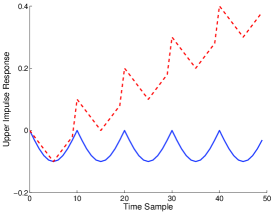
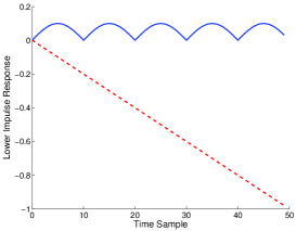
(a)                                            (b)

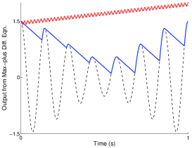
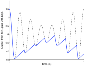
(c)                                            (d)

Figure 2: Responses of DTI or ETI systems described by the recursive max-sum equation (116) or its min-sum version (124); in all cases $m=0$, $b_{0}=0$. (a) Impulse response (first 50 samples) of a $n=11^{th}$-order DTI system for two coefficient sequences $\{a_{k}\}$: in solid line $a_{k}=-\sin(\pi(k-1)/10)/10$ for $k=1,..,10$ and $a_{11}=0$, whereas in dash line $a_{k}^{\prime}=(|k-6|-5)/50$ for $k=1,..,10$ and $a_{11}^{\prime}=0.1$. (b) Dual impulse response (first 50 samples) of a $11^{th}$-order recursive ETI system for two coefficient sequences: in solid line $a_{k}=\sin(\pi(k-1)/10)/10$ for $k=1,..,10$ and $a_{11}=0$, whereas in dash line $a_{k}^{\prime}=(|k-6|-5)/50$ for $k=1,..,11$. (c) Output signals from two DTI systems whose input (dashed line) is an amplitude-modulated sine. The first output (solid blue line) is from the stable system $y(t)=\max[y(t-1)+a_{1},u(t)]$ with $a_{1}=-0.008$. The second output (dotted red line) is from the unstable system that generated the unstable impulse response of (a). (d) Input signal as in (c) and output from the min-sum system $y(t)=\min[y(t-1)-a_{1},u(t)]$.

9.1.2 Dynamic Programming

The max-sum or min-sum recursive equations can also express various forms of dynamic programming, either of maximizing some gain or minimizing some cost or distance [Bert12, BCOQ01]. For example consider (8) and assume that $a_{ij}$ is the transition gain from state $i$ to state $j$ between two consecutive time instants and that $x_{i}(t)$ represents the maximum possible gain to reach state $i$ in $t$ steps starting from some initial state at $t=0$. Then (8) with a transposed transition matrix, i.e. the max-sum system

$$\boldsymbol{x}(t)=\boldsymbol{A}^{T}\boxplus\boldsymbol{x}(t-1),\quad\boldsymbol{x}(0)=[0,-\infty,...,-\infty]^{T},$$ (125)

models a dynamic programming algorithm where, starting from state 1 with zero gain, we move from state to state aiming at solving the above optimization problem by sequentially maximizing the gain. The optimum path can be found by backtracking.

Instead of max-sum, there is also a max-product example of dynamic programming presented in Sec. 9.2.1. Other abstract models of dynamic programming have been studied in [VePo87].

9.1.3 Distance maps and min-plus recursions

The min-sum version of (8) models shortest path problems. Given a 2D rectangular field $f:\mathcal{V}\rightarrow\mathbb{R}$ on a grid $\mathcal{V}$ of $M\times N$ pixels, its weighted distance transform is defined by

$$D_{f}(i,j)=\bigwedge_{(k,\ell)\in\mathcal{V}}d(i-k,j-\ell)+f(k,\ell)$$ (126)

where $d(\cdot)$ is the Euclidean distance. For various cases of $f$, the above distance computation problem is at the heart of several well-known optimization problems [FeHu04a],[Tsit95]. If $D_{f}$ is available, we can solve the shortest path problem from any point by following the gradient of the distance map. If $f$ equals $q^{\prime}_{S}$, which is the lower indicator function of a set $S\subseteq\,\mathcal{V}$ with values 0 on $S$ and $+\infty$ on $\mathcal{V}\setminus S$, then $D_{f}$ becomes the distance transform of the set $S$:

$$D_{S}(i,j)=\min_{(k,\ell)\in S}\|i-k,j-\ell\|$$ (127)

which measures distances from $S$ out into its containing field. Consider indexing rowwise the 2D rectangular grid $\mathcal{V}$ of $M\times N$ pixels $(i,j)$ as a 1D sequence of points $t=N(i-1)+j$, $i=1,...,M,j=1,...,N$. A good approximation to the Euclidean distance function $D_{S}(t)$ is to compute the chamfer distance [Borg84] by propagating a $3\times 3$ mask (8-pixel neighborhood) of local distance steps $(a,b)$. A serial implementation is an iterative algorithm where the 8-pixel neighborhood is partitioned into two 4-pixel subneighborhoods, and each new array of results sequentially passes through recursive infimal convolutions $y_{i}(t)$, $i=1,2,3,...$, which for odd $i$ are a forward pass with the submask of Fig. 3(a) scanning rowwise the 2D field from top to bottom and for even $i$ are a backward pass with the reflected submask in the reverse scanning order. The $i$-th forward pass is described by the min-sum difference equation

$$y_{i}(t)=[\bigwedge_{k=1}^{N+1}w_{k}+y_{i}(t-N+k-2)]\wedge u_{i-1}(t)$$ (128)

where $w_{1}=b,w_{2}=a,w_{3}=b,w_{N+1}=a$ and all other $w_{k}$ are $+\infty$, $u_{0}=q^{\prime}_{S}$ and $u_{i}=y_{i}$ for $i\geq 1$. Its dynamics can be modeled by the min-sum version of the general state equations (6). It admits a state space model as in (123) with $n=N+1$ states $x_{k}(t)=y(t-N+k-2)$, the only differences being that the null elements ($-\infty$) in the sparse system matrices should be replaced with $+\infty$, and all elements in the last row of $\boldsymbol{A}$ and in $\boldsymbol{C}$ are $+\infty$ except at four positions ($k=1,2,3,N+1$) where they are equal to the corresponding local distances. The source set $S$ could be a small region from which we propagate distances; see Fig. 3(b,c). If the field contains impenetrable obstacles (like ‘walls’) $W$, distance maps can be produced that account for this impenetrability, and then shortest paths can be found that avoid collision with the walls, which is useful in robotics [VDVG86]. This can be done by imposing in each iteration values $+\infty$ at all points of the wall $W$. The algorithm (128) generally converges to $D_{S}(t)=\lim y_{i}(t)$, and the number of required passes is two if there are no obstacles; see Fig. 3(d). For a 1D sequence $S$ of points, we need only two passes as the following example illustrates with recursions $y_{1}(t)=\min[y_{1}(t-1)+1,u_{0}(t)]$ and $y_{2}(t)=\min[y_{2}(t+1)+1,y_{1}(t)]$:

$$\begin{array}[]{|c|c|c|c|c|c|c|c|c|c|c|c|c|}\hline\cr u_{0}&\infty&0&\infty&\infty&\infty&0&\infty&\infty&\infty&\infty&\infty&0\\ \hline\cr y_{1}&\infty&0&1&2&3&0&1&2&3&4&5&0\\ \hline\cr y_{2}&1&0&1&2&1&0&1&2&3&2&1&0\\ \hline\cr\end{array}$$

Note that both recursive equations are stable min-plus systems.

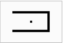
(a)    (b)

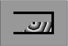
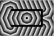
(c) (d)

Figure 3: (a) Coefficient submask for forward pass of sequential distance transform. (b) Source set $S$ and the obstacle wall set $W$. (c) First (forward) pass of constrained distance transform with steps $(a,b)=(24,34)/25$. (d) Fourth (backward) pass and final result, shown with gray values modulo a constant.

9.2 Max-Product systems

Another class of nonlinear dynamical systems is obtained by using the nonnegative numbers $\mathcal{K}=[0,+\infty]$ as scalars, the standard product ($\times$) as scalar ‘multiplication’, and the following max-product $\boxtimes$ and its dual $\boxtimes^{\prime}$ as generalized matrix ‘multiplications’ in (2) and (6):

$$\boldsymbol{C}=\boldsymbol{A}\boxtimes\boldsymbol{B}=[c_{ij}] c_{ij}={\displaystyle\bigvee_{k=1}^{n}}a_{ik}\times b_{kj}$$ , (129)

$$\boldsymbol{C}=\boldsymbol{A}\boxtimes^{\prime}\boldsymbol{B}=[c_{ij}] c_{ij}={\displaystyle\bigwedge_{k=1}^{n}}a_{ik}\times^{\prime}b_{kj}$$ , (130)

The scalar multiplications $\times$ and $\times^{\prime}$ coincide over $(0,+\infty)$, but $a\times 0=0$ and $a\times^{\prime}(+\infty)=+\infty$ for all $a\in[0,+\infty]$. Henceforth, we shall use the same symbol $\times$ for both scalar operations. Here the scalar arithmetic is based on the max-times clog $([0,\infty],\vee,\wedge,\times)$. This max-product formalism can model dynamical systems whose inputs, states, and outputs are constrained to be nonnegative. Note that there is an isomorphism between the max-sum and the max-product systems because, if we have the following max-product state equations

$$\boldsymbol{x}(t)=\boldsymbol{A}\boxtimes\boldsymbol{x}(t-1)\vee\boldsymbol{B}\boxtimes\boldsymbol{u}(t)$$ (131)

and take logarithms of both sides element-wise, we obtain the max-sum equations

$$\log\boldsymbol{x}(t)=\log\boldsymbol{A}\boxplus\log\boldsymbol{x}(t-1)\vee\log\boldsymbol{B}\boxplus\log\boldsymbol{u}(t)$$ (132)

Such systems have found applications in speech recognition and other natural language processing tasks using finite-state automata [MPR02, HoNa13], in computer vision [FeHu04a], the max-product algorithm in belief propagation [Pear88] and related probabilistic graphical models used in machine learning [Bish06].

9.2.1 Viterbi Algorithm and HMMs

Given a time sequence of observations (feature vectors) $\boldsymbol{O}=(\boldsymbol{o}_{t})_{t=0}^{T}$, a fundamental problem in their statistical modeling using hidden Markov models (HMMs) [RaJu93] with $n$ discrete states $\{1,...,n\}$ is to find the best sequence of states $\hat{\boldsymbol{s}}=(s_{0},s_{1},...,s_{T})$ that maximizes the probability $\mathrm{Pr}(\boldsymbol{O},\boldsymbol{s}|\boldsymbol{\theta})$, where $\boldsymbol{\theta}=([\pi_{i}],[a_{ij}],[p_{i}])$ are the HMM parameters: $\pi_{i}$ are the initial state probabilities at $t=0$, $a_{ij}=\mathrm{Pr}(s_{t}=j|s_{t-1}=i)$ are state transition probabilities, and $p_{i}(t)$ are the state-conditional observation probabilities $p(\boldsymbol{o}_{t}|s_{t}=i)$ often modeled by Gaussian Mixture models (GMMs). Consider the highest probability of a single partial state sequence ending at state $i$ at time $t$ and accounting for the first $t+1$ observations:

$$x_{i}(t)=\max_{s_{0},...,s_{t-1}}\mathrm{Pr}[s_{0},...,s_{t-1},s_{t}=i,\boldsymbol{o}_{0},...,\boldsymbol{o}_{t}|\boldsymbol{\theta}]$$ (133)

One solution is to use the Viterbi algorithm to find the max global score

$$\hat{P}=\mathrm{Pr}(\boldsymbol{O},\hat{\boldsymbol{s}}|\boldsymbol{\theta})=\max_{i}x_{i}(T)$$ (134)

and then find the optimal state sequence via backtracking. This is essentially dynamic programming and amounts to evolving the following system, for $t=1,...,T$,

$$\begin{array}[]{rcl}x_{i}(t)&=&\left(\bigvee_{j=1}^{n}a_{ji}x_{j}(t-1)\right)\cdot p_{i}(t)\\ y(t)&=&\bigvee_{i=1}^{n}x_{i}(t)\end{array}$$ (135)

with $x_{i}(0)=\pi_{i}p_{i}(0)$. Then, this is a max-product system with matrices $\boldsymbol{A}(t)=[a_{ji}]p_{i}(t)$, $\boldsymbol{C}=[1,1,...,1]$ and zero input. The Viterbi score is given by the final output $\hat{P}=y(T)$.

9.2.2 Attention Control and Multimodal Saliencies

Assume a video sequence of audio-visual (AV) events each to be scored with some degree of saliency in $[0,1]$ where ‘saliency’ is some bottom-up low-level sensory form of attention by a human watching this video. The states $x_{1},x_{2},x_{3},x_{4}$ represent time-evolving mono- or multi-modal saliencies, where 1=audio, 2=visual, 3=audiovisual, and 4=non-salient. Peaks in these saliency trajectories signify important events, which can be automatically detected and produce video summaries that agree well with human attention [Eva+13]. The following state equations are a possible max-product dynamical model we have proposed for the evolution of these saliency states [MaKo15]:

$$x_{i}(t)=\left(\bigvee_{j=1}^{4}a_{ji}x_{j}(t-1)\right)\star p_{i}(t)\vee\left(\bigvee_{j=1}^{4}b_{ij}u_{j}(t)\right)$$ (136)

for state $i=1,2,3,4$. The constants $a_{ij}$ represent state transitions probabilities and $p_{i}(t)=p(\boldsymbol{o}_{t}|s_{t}=i)$ denote the probabilities of observed low-level feature vectors $\boldsymbol{o}_{t}$ while being at the $i$-th saliency state. We assume that the parameters $a_{ij},\ b_{ij}$ and $p_{i}(t)$ are given.

Given a time sequence of such observations $(\boldsymbol{o}_{t})$ one can fit HMMs to these data using maximum likelihood. Then, the first term in the RHS of (136) models the evolution of the Viterbi dynamic programming algorithm (135) used in HMMs. For example, if the inputs $u_{i}(t)$ are all null, then the single output $y(t)=\bigvee_{i}x_{i}(t)$ computes the Viterbi score (134). One main difference of our system (136) with the Viterbi algorithm (135) is that we have the probability-like signals $u_{i}(t)$ which can act as control inputs coming possibly from previous human attention states or higher-level events; e.g. detected human faces, voice activity, or text semantics. Another difference is that the outputs of the dynamical system can be various min-max combinations of the saliency states of various modalities; e.g. the single output

$$y(t)=c_{1}x_{1}(t)\vee c_{2}x_{2}(t)\vee d_{1}u_{1}(t)\vee d_{2}u_{2}(t)$$ (137)

forms a weighted max-product fusion of the audio and visual saliencies as well as the two corresponding inputs. In such modality and input combinations, the max rule can be replaced by min too. A third difference is that the data-controlled probabilities $p_{i}(t)$ can enter not only via multiplication but also via any commutative binary operation $\star$ that distributes over maximum. If $\star=\max$, then the $p_{i}(t)$ can be viewed as control inputs. Finally, our CWL theoretical formulation allows us to also compute analytically the responses of such max-product dynamical systems; see Sec. 4.

In our experiments [MaKo15] we estimated the state transition probabilities $a_{ij}$ using the EM algorithm on some training data from movie videos. For estimating the observation data probabilities $p_{i}(t)$ we fitted GMMs to audio and visual feature vectors extracted from the video data at each frame $t$. Figure 4 shows the results (on testing data from the same movie videos) of various approaches we have initiated to track the joint audio-visual (AV) saliency state and compare it (i) with human annotations, i.e. binary AV saliency manually annotated by a human who observed these movie videos, and (ii) with an AV saliency automatically computed in [Eva+13] by fusing saliencies of the audio and visual streams measured from monomodal cues. Our ongoing research goal here is to develop a computational model that can track human attention in the form of audio-visual saliency states based on multimodal sensory inputs. As shown in Fig. 4 and explained numerically in [MaKo15], our results using the max-product dynamical system are encouraging; they can track audio-visual saliencies with smaller error than bottom-up feature-based local measurements and can improve with higher-level control input.

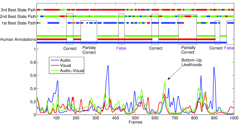
Figure 4: Evolution of audio (blue), visual (red) and audio-visual (green) bottom-up likelihoods computed from observed features. We also see the human annotations and the 3-Best state paths using the max-product dynamical system (136) with $\star$ being product operation and two control inputs $u_{1}(t)$ and $u_{2}(t)$ providing binary information from voice and face detection respectively. (This figure is best viewed in color.)

9.3 Max-$T$norm systems and Fuzzy Markov Chains

There are many types of nonlinear dynamical systems where the elements of the state, input and output vectors represent probabilities or memberships. Examples include probabilistic or fuzzy control systems [AvSa02, KlYu95, MST00], fuzzy image convolutions [BlMa95, Mara05a], as well as certain types of neural nets with max-min combinations of inputs [KlYu95, YaMa95]. The dynamics of large classes of such systems can be described by the general model if we restrict the set of scalars to be $\mathcal{K}=[0,1]$ and use as scalar ‘multiplication’ $a\star b=T(a,b)$ a fuzzy intersection norm [KlYu95], i.e., a binary operation $T:[0,1]^{2}\rightarrow[0,1]$ that is i) commutative, ii) associative, iii) increasing and iv) satisfies the boundary condition $T(a,1)=a$ for all $a\in[0,1]$. This is also known as ‘triangular norm’ (t-norm) in statistics. We also require that $T$ is continuous, which makes it a scalar dilation [MST00]. As dual ‘scalar multiplication’, we use a continuous binary operation $U(a,b)=a\star^{\prime}b$ that satisfies (i)-(iii) and the dual boundary condition $U(a,0)=a$. This is a fuzzy union norm [KlYu95], also known as ‘t-conorm’, and is a scalar erosion on $[0,1]$. Choosing in the general lattice dynamical model the above set of scalars and ‘multiplications’ among them creates the case of max-$T$norm and min-$U$norm systems, obtained by replacing in (2) and (6) the general max-$\star$ matrix multiplication and its dual with the following versions:

$$\boldsymbol{C}=\boldsymbol{A}\ \framebox(0.0,0.0)[bl]{\star}\ \boldsymbol{B}=[c_{ij}] c_{ij}={\displaystyle\bigvee_{k=1}^{n}}T(a_{ik},b_{kj})$$ , (138)

$$\boldsymbol{C}=\boldsymbol{A}\ \framebox(0.0,0.0)[bl]{\star}\,^{\prime}\ \boldsymbol{B}=[c_{ij}] c_{ij}={\displaystyle\bigwedge_{k=1}^{n}}U(a_{ik},b_{kj})$$ , (139)

Usually we select $U(a,b)=a\star^{\prime}b=T^{\ast}(a,b)$ where $T^{\ast}$ is the conjugate norm obtained via fuzzy complementation:

$$T^{\ast}(a,b)=1-T(1-a,1-b)$$ (140)

then $(T,T^{\ast})$ form a negation duality, but not an adjunction. The most well-studied choice for the $T$ norm and its dual norm $T^{\ast}$ are the min and max operations, respectively. Another known case is for $T$ to equal the product operation. Table 4 shows these cases and their adjoints so that $(T,\zeta)$ and $(\eta,T^{\ast})$ are scalar adjunctions. There are also numerous other choices.

Table 4: T-norms, Conorms and their Adjoints

t-norm adjoint t-norm t-conorm adjoint t-conorm $T(a,v)$ $\zeta(a,w)$ $U={T}^{\ast}(a,w)$ $\eta(a,v)$ $\min(a,v)$ $\max([w\geq a],w)^{\dagger}$ $\max(a,w)$ $\min([v>a],v)$ $a\cdot v$ $\min(w/a,1)$ $a+w-a\cdot w$ $\max(\frac{v-a}{1-a},0)$

 
${}^{\dagger}\ [P]$ is the Iverson bracket with value 1 (0) if $P$ is true (false).

An application of the above ideas to state-space description and control of fuzzy dynamical systems is presented in [MST00]. Further, dynamical systems with states $\boldsymbol{x}(t)\in[0,1]^{n}$ and transition rule based on the max-min matrix ‘multiplication’ ($\star=\min$)

$$𝒙(t+1)=𝑨\text{<svg version="1.1" width="" height="" overflow="visible" id="S9.E141.m1.1.1a" xref="S9.E141.m1.1.1e.cmml"><g transform="translate(0,0) scale(1,-1)" id="S9.E141.m1.1.1b" xref="S9.E141.m1.1.1e.cmml"><rect fill="none" height="4.7pt" stroke="\#000000" stroke-width="0.4" width="5.0pt" x="0" y="0" id="S9.E141.m1.1.1c" xref="S9.E141.m1.1.1e.cmml"></rect><g class="makebox" transform="translate(0,0)" id="S9.E141.m1.1.1d" xref="S9.E141.m1.1.1e.cmml"></g></g></svg>}$$ (141)