An integral equation formulation for rigid bodies in Stokes flow in three dimensions

Abstract

We present a new derivation of a boundary integral equation (BIE) for simulating the three-dimensional dynamics of arbitrarily-shaped rigid particles of genus zero immersed in a Stokes fluid, on which are prescribed forces and torques. Our method is based on a single-layer representation and leads to a simple second-kind integral equation. It avoids the use of auxiliary sources within each particle that play a role in some classical formulations. We use a spectrally accurate quadrature scheme to evaluate the corresponding layer potentials, so that only a small number of spatial discretization points per particle are required. The resulting discrete sums are computed in $\mathcal{O}(n)$ time, where $n$ denotes the number of particles, using the fast multipole method (FMM). The particle positions and orientations are updated by a high-order time-stepping scheme. We illustrate the accuracy, conditioning and scaling of our solvers with several numerical examples.

1 Introduction

In viscous flows, the mobility problem consists of computing the translational and rotational velocities $(\boldsymbol{[}v]_{i},\boldsymbol{[}\omega]_{i})$ induced on a collection of $n$ rigid bodies when prescribed forces and torques $(\boldsymbol{[}F]_{i},\boldsymbol{[}T]_{i})$ are specified on each one. The Stokes equations, which are linear, govern the ambient viscous fluid at vanishing Reynolds number limit. Thereby, there exists a well-defined mobility matrix denoted by $M$ such that

$$\boldsymbol{[}V]=M\boldsymbol{[}F]\,,$$ (1.1)

where $\boldsymbol{[}V]=(\boldsymbol{[}v]_{1},\boldsymbol{[}\omega]_{1},\dots,\boldsymbol{[}v]_{n},\boldsymbol{[}\omega]_{n})$ and $\boldsymbol{[}F]=(\boldsymbol{[}F]_{1},\boldsymbol{[}T]_{1},\dots,\boldsymbol{[}F]_{n},\boldsymbol{[}T]_{n})$.

Reformulating the problem as an integral equation has several advantages over direct discretization of the governing partial differential equations themselves. First, integral equation methods require discretization of the particle boundaries alone, which leads to an immediate reduction in the size of the discretized linear system. Equally important, carefully chosen integral representations result in well-conditioned linear systems, while discretizing the Stokes equations directly leads to highly ill-conditioned systems. Moreover, the integral representation can be chosen to satisfy the far field boundary conditions necessary to model an open system, thereby eliminating the need for artificial truncation of the computational domain. Lastly, combining high-order quadrature methods and suitable fast algorithms, boundary integral equations for complex geometries can be solved to high accuracy in optimal or near optimal time [15, 6, 25, 30, 42].

A variety of integral representations for the mobility problem have been introduced, often in the form of first kind integral equations [9] or second kind integral equations with $n$ additional unknowns and an equal number of additional constraints [24]. While these have been shown to be very effective, it is advantageous (when $n$ is large and the rigid bodies have complicated shape) to work with well-conditioned second kind boundary integral formulations which are free of additional constraints. Such schemes have been developed earlier [18], using the Lorentz reciprocal identity. The equation which we derive below in Section 2 is essentially the same, but obtained using a different principle - namely that the interior of a rigid body must be stress free. The mobility problem can also be solved using a double layer representation that doesn’t involve additional unknowns. For a detailed discussion of the latter approach, we refer the reader to [33, 1]. Our formulation has the advantage that certain derivative quantities, such as fluid stresses, can be computed using integral operators with weakly singular kernels instead of hypersingular ones, simplifying the quadrature issues.

Based on this formulation, we present a numerical algorithm in Section 3 to solve the mobility problem and evolve the position and orientation of the rigid bodies. In Section 4, we discuss several applications and present results from our numerical experiments (a sample simulation with large $n$ is depicted in Figure 1).

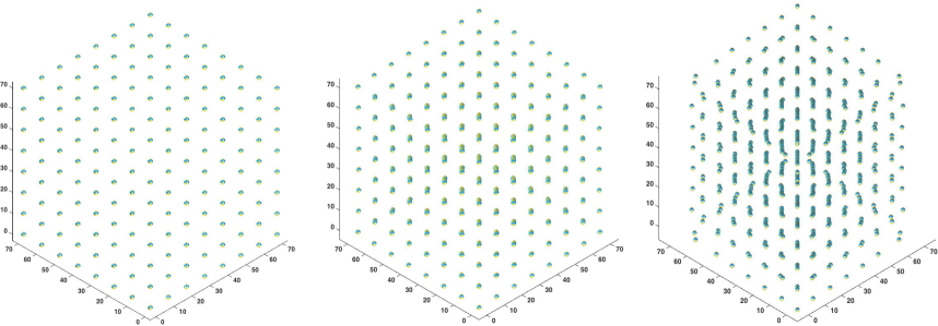
Figure 1: Self-assembly of chains in a magnetorheological fluid. Snapshots from a simulation of a cubic lattice of $512$ paramagnetic spheres subjected to a uniform magnetic field $\boldsymbol{[}H]_{0}$ in a Stokesian flow. We use spherical harmonic expansions of degree $p=8$ to represent functions on each sphere, requiring a total of $294912$ degrees-of-freedom per time-step to compute hydrodynamic and magnetic interactions. At each time-step, a magnetostatic problem is solved for the current particle configuration; the Maxwell stresses thus obtained at the particle boundaries give rise to a mobility poblem (details in Section 4). Our BIE formulations for both the fluid velocity and magnetic potential problems lead to well-conditioned linear systems. Summation of far-field interactions is accelerated via Stokes and Laplace FMMs [12]. On an average, this simulation took $5$ minutes per time-step on a single node with Intel Xeon E–$2690$ v$2$($3.0$ GHz) processor and $24$ GB of RAM.

2 The mobility problem

Let $\{D_{i}\}_{i=1}^{n}$ be a set of $n$ disjoint rigid bodies in $\mathbb{R}^{3}$ with boundaries $\Gamma_{i}$. Let $\boldsymbol{[}F]_{i},\boldsymbol{[}T]_{i}$ denote the force and torque exerted on $D_{i}$, and let $\boldsymbol{[}v]_{i},\boldsymbol{[}\omega]_{i}$ denote the translational and rotational velocity of $D_{i}$. Let $E$ be the domain exterior to all of the rigid bodies $\{D_{i}\}$, and assume that the fluid in $E$ is governed by Stokes flow with viscosity $\mu=1$. For a given velocity field $\boldsymbol{[}u](\boldsymbol{[}x])\in\mathbb{R}^{3}$ at a point $\boldsymbol{[}x]\in E$, we denote the corresponding fluid pressure, strain and stress tensors by $p$, $e\left(\boldsymbol{[}u]\right)$ and $\sigma$, respectively. On the surface of the rigid bodies, $\boldsymbol{[}f]=\sigma\cdot\boldsymbol{[}n]$ denotes the surface force or surface traction exerted by the fluid on the rigid body $D_{i}$. For the sake of simplicity, we assume there are no volume forces. The governing equations for the mobility problem are then given by:

$$-\Delta\boldsymbol{[}u]+\boldsymbol{[}\nabla]p=\boldsymbol{[}0],\ \ \ \ \boldsymbol{[}\nabla]\cdot\boldsymbol{[}u]=0\ \ \forall\boldsymbol{[}x]\in E,$$ (2.1)

$$\boldsymbol{[}u](\boldsymbol{[}x])=\boldsymbol{[}v]_{i}+\boldsymbol{[}\omega]_{i}\times(\boldsymbol{[}x]-\boldsymbol{[}x]^{c}_{i})\ \ \forall\boldsymbol{[}x]\in\Gamma_{i},$$ (2.2)

$$\int_{\Gamma_{i}}\boldsymbol{[}f]\,dS_{y}=\int_{\Gamma_{i}}\sigma\cdot\boldsymbol{[}n]\,dS_{y}=-\boldsymbol{[}F]_{i},\ \ \ \int_{\Gamma_{i}}(\boldsymbol{[}x]-\boldsymbol{[}x]^{c}_{i})\times\boldsymbol{[}f]\,dS_{y}=-\boldsymbol{[}T]_{i},$$ (2.3)

$$\boldsymbol{[}u](\boldsymbol{[}x])\rightarrow\boldsymbol{[}0]\ \ \mathrm{as}\ \ |\boldsymbol{[}x]|\rightarrow\infty.$$ (2.4)

It should be noted that the forces and torques, $\boldsymbol{[}F]_{i}$, and $\boldsymbol{[}T]_{i}$ are known and the translational and rotational velocities $\boldsymbol{[}v]_{i}$, and $\boldsymbol{[}\omega]_{i}$ are unknown.

Before turning to the integral equation, however, we state and prove a simple uniqueness result. To prove uniqueness, we need the following lemma contained in [33]

Lemma 1.

Let $\boldsymbol{[}u]$ solve Stokes equation in the exterior domain $E\subseteq\mathbb{R}^{3}$ defined above, satisfying the condition (2.4). Let $B_{R}\left(0\right)$ be the ball of radius $R$ centered at the origin and let $\partial B_{R}\left(0\right)$ be its boundary. Then, there exist $M,R_{0}$ such that $\sup_{\partial B_{R}\left(0\right)}\left|\boldsymbol{[}u]\right|\leq\frac{M}{R}$ and $\sup_{\partial B_{R}\left(0\right)}\left|\sigma\right|\leq\frac{M}{R^{2}}$ for all $R\geq R_{0}$. From these decay conditions at $\infty$ it also follows that

$$\lim_{R\to\infty}\int_{\partial B_{R}\left(0\right)}\left(\boldsymbol{[}u],\boldsymbol{[}f]\right)\,dS_{y}\to 0\,.$$ (2.5)

Lemma 2.

If $\boldsymbol{[}u]$ satisfies equations (2.2), and (2.3) with $\boldsymbol{[}F]_{i}=\mathbf{0}$ and $\boldsymbol{[}T]_{i}=\mathbf{0}$ then

$$\int_{\Gamma_{i}}\left(\boldsymbol{[}u],\boldsymbol{[}f]\right)\,dS_{y}=0\,.$$ (2.6)

Proof.

$$\int_{\Gamma_{i}}\left(\boldsymbol{[}u],\boldsymbol{[}f]\right)\,dS_{y}=\int_{\Gamma_{i}}\left(\boldsymbol{[}v]_{i}+\boldsymbol{\omega}_{i}\times\left(\boldsymbol{[}x]-\boldsymbol{[}x]^{c}_{i}\right),\boldsymbol{[}f]\right)\,dS_{y}=-\left(\boldsymbol{[}u]_{i},\boldsymbol{[}F]_{i}\right)-\left(\boldsymbol{[}\omega]_{i},\boldsymbol{[}T]_{i}\right)=0\,.$$ (2.7)

∎

Lemma 3.

If $\boldsymbol{[}u](\boldsymbol{[}x])$ satisifies equations (2.1), (2.2), (2.3) and (2.4) with $\boldsymbol{[}F]=\mathbf{0}$, then $\boldsymbol{[}u](\boldsymbol{[}x])\equiv\mathbf{0}$ in $E$.

Proof.

Let $\left\langle\cdot,\cdot\right\rangle:\mathbb{R}^{3\times 3}\times\mathbb{R}^{3\times 3}$ be the Frobenius inner product. For large enough $R$,

$$\int_{E\cap B_{R}\left(0\right)}\left\langle e\left(\boldsymbol{[}u]\right),e\left(\boldsymbol{[}u]\right)\right\rangle dV =\int_{E\cap B_{R}\left(0\right)}\left\langle D\boldsymbol{[}u],e\left(\boldsymbol{[}u]\right)\right\rangle dV$$

$$=\int_{\partial(E\cap B_{R}\left(0\right))}\left(\boldsymbol{[}u],e\left(\boldsymbol{[}u]\right)\cdot\mathbf{n}\right)\,dS_{y}-\frac{1}{2}\int_{E\cap B_{R}\left(0\right)}\left(\boldsymbol{[}u],\Delta\boldsymbol{[}u]\right)dV$$

$$=\int_{\partial(E\cap B_{R}\left(0\right))}\left(\boldsymbol{[}u],e\left(\boldsymbol{[}u]\right)\cdot\mathbf{n}\right)\,dS_{y}-\frac{1}{2}\int_{E\cap B_{R}\left(0\right)}\left(\boldsymbol{[}u],\nabla p\right)dV$$

$$=\frac{1}{2}\int_{\partial\left(E\cap B_{R}\left(0\right)\right)}\left(\boldsymbol{[}u],\left(-p\left[\begin{array}[]{cc}1&0\\ 0&1\end{array}\right]+2e\left(\boldsymbol{[}u]\right)\right).\mathbf{n}\right)\,dS_{y}\quad$$

$$=-\frac{1}{2}\sum_{i=1}^{N}\int_{\Gamma_{i}}\left(\boldsymbol{[}u],\boldsymbol{[}f]\right)\,dS_{y}+\frac{1}{2}\int_{\partial B_{R}\left(0\right)}\left(\boldsymbol{[}u],\boldsymbol{[}f]\right)\,dS_{y}$$

$$=\frac{1}{2}\int_{\partial B_{R}\left(0\right)}\left(\boldsymbol{[}u],\boldsymbol{[}f]\right)\,.$$

using (2.1) and Lemma 2. Taking the limit as $R\to\infty$ in the above expression and using equation (2.5), we get

$$e\left(\boldsymbol{[}u]\right)\equiv\left[\begin{array}[]{cc}0&0\\ 0&0\end{array}\right]\quad\boldsymbol{[}x]\in E\,.$$ (2.8)

Thus, $\boldsymbol{[}u]$ is a rigid body motion. Since $\boldsymbol{[}u](\boldsymbol{[}x])\to\mathbf{0}$ as $\left|\boldsymbol{[}x]\right|\to\infty$, we conclude that $\boldsymbol{[}u]\equiv\mathbf{0}$. ∎

Our integral equation is based on representing the solution $\boldsymbol{[}u]$ as the sum of two fields: an incident field $\boldsymbol{[}u]_{inc}$ that accounts for the net force and torque conditions in Eq. (2.3), and a scattered field $\boldsymbol{[}u]_{sc}$ with zero net forces and torques that enforces that $\boldsymbol{[}u]$ is a rigid body motion at each boundary (Eq. (2.2)). As noted in [36, 37], if the incident field is defined by uniformly distributed forces and torques, then determination of the scattered field can be interpreted as redistributing those uniformly placed surface forces so as to eliminate any interior stress.

2.1 Notation and preliminaries

Let $\Gamma$ be a smooth surface in $\mathbb{R}^{3}$, $D^{\mp}$ denote the domains inside and outside $\Gamma$, and $\boldsymbol{[}n]\left(\boldsymbol{[}x]\right)$ the unit outward normal vector at $\boldsymbol{[}x]\in\Gamma$. Let $G_{i,j}(\boldsymbol{[}x],\boldsymbol{[}y])$ be the Stokeslet, that is, the fundamental solution to the Stokes equations in free space in $\mathbb{R}^{3}$, given by:

$$G_{i,j}(\boldsymbol{[}x],\boldsymbol{[}y])=\frac{1}{8\pi}\left(\frac{\delta_{i,j}}{|\boldsymbol{[}x]-\boldsymbol{[}y]|}+\frac{(x_{i}-y_{i})(x_{j}-y_{j})}{|\boldsymbol{[}x]-\boldsymbol{[}y]|^{3}}\right)\,.$$ (2.9)

Then the single layer potential operator for the Stokes equation $\mathcal{[}S]_{\Gamma}$ is given by

$$\mathcal{[}S]_{\Gamma}[\boldsymbol{[}\mu]](\boldsymbol{[}x])_{i}=\int_{\Gamma}G_{i,j}(\boldsymbol{[}x],\boldsymbol{[}y])\mu_{j}(\boldsymbol{[}y])\,dS_{y}\,.$$ (2.10)

If we let $\boldsymbol{[}f]$ denote the surface traction corresponding to $\boldsymbol{[}u]=\mathcal{[}S]_{\Gamma}[\boldsymbol{[}\mu]]$, then from standard jump relations for the single layer potential, we have:

$$f^{\pm}_{i}(\boldsymbol{[}x])=\mp\frac{1}{2}\mu_{i}(\boldsymbol{[}x])+n_{k}(\boldsymbol{[}x])\mathchoice{{\vbox{\hbox{$\textstyle-$}}\kern-4.86108pt}}{{\vbox{\hbox{$\scriptstyle-$}}\kern-3.25pt}}{{\vbox{\hbox{$\scriptscriptstyle-$}}\kern-2.29166pt}}{{\vbox{\hbox{$\scriptscriptstyle-$}}\kern-1.875pt}}\!\int_{\Gamma}T_{i,j,k}(\boldsymbol{[}x],\boldsymbol{[}y])\mu_{j}(\boldsymbol{[}y])\,dS_{y}\,,$$ (2.11)

where $\mathchoice{{\vbox{\hbox{$\textstyle-$}}\kern-4.86108pt}}{{\vbox{\hbox{$\scriptstyle-$}}\kern-3.25pt}}{{\vbox{\hbox{$\scriptscriptstyle-$}}\kern-2.29166pt}}{{\vbox{\hbox{$\scriptscriptstyle-$}}\kern-1.875pt}}\!\int$ is the principal value integral, and $T_{i,j,k}$ is the traction kernel given by:

$$T_{i,j,k}(\boldsymbol{[}x],\boldsymbol{[}y])=-\frac{3}{4\pi}\frac{(x_{i}-y_{i})(x_{j}-y_{j})(x_{k}-y_{k})}{|\boldsymbol{[}x]-\boldsymbol{[}y]|^{5}}$$ (2.12)

The interior forces and torques are zero, while the exterior ones are equal to the corresponding moments for $\boldsymbol{[}\mu]$:

$$\int_{\Gamma_{i}}\boldsymbol{[}f]^{-}(\boldsymbol{[}y])\,dS_{y}=0\ \ \ \int_{\Gamma_{i}}(\boldsymbol{[}y]-\boldsymbol{[}x]^{c}_{i})\times\boldsymbol{[}f]^{-}(\boldsymbol{[}y])\,dS_{y}=0$$ (2.13)

$$\int_{\Gamma_{i}}\boldsymbol{[}f]^{+}(\boldsymbol{[}y])\,dS_{y}=-\int_{\Gamma}\boldsymbol{[}\mu](\boldsymbol{[}y])\,dS_{y}\ \ \ \int_{\Gamma_{i}}(\boldsymbol{[}y]-\boldsymbol{[}x]^{c}_{i})\times\boldsymbol{[}f]^{+}(\boldsymbol{[}y])\,dS_{y}=-\int_{\Gamma_{i}}(\boldsymbol{[}y]-\boldsymbol{[}x]^{c}_{i})\times\boldsymbol{[}\mu](\boldsymbol{[}y])\,dS_{y}\,.$$ (2.14)

Finally,

$$\left|\mathcal{[}S]_{\Gamma}[\boldsymbol{[}\mu]](\boldsymbol{[}x])\right|\to 0\ \ \ \text{as}\ \left|\boldsymbol{[}x]\right|\to\infty\,.$$ (2.15)

2.2 The “incident” and “scattered” fields

We first define an incident field $\boldsymbol{[}u]_{inc}$ which is a solution to the Stokes equations in $E$ (Equations (2.1),(2.4)) and satisfies the specified net forces and torques on each boundary $\Gamma_{i}$ (Eq. (2.3)). Given a force density $\boldsymbol{[}\rho](\boldsymbol{[}x])$ in $\Gamma=\cup_{i=1}^{n}\Gamma_{i}$, with $\boldsymbol{[}\rho]_{i}=\boldsymbol{[}\rho]|_{\Gamma_{i}}$, we let $\boldsymbol{[}u]_{inc}=\mathcal{[}S]_{\Gamma}[\boldsymbol{[}\rho]]$. Since the Stokes equations and conditions at infinity are immediately satisfied, according to Eq. (2.14), we only need to choose a $\boldsymbol{[}\rho]$ such that

$$\boldsymbol{[}F]_{i}=\int_{\Gamma_{i}}\boldsymbol{[}\rho]_{i}(\boldsymbol{[}y])\,\ dS_{y}\ \,\ \boldsymbol{[}T]_{i}=\int_{\Gamma_{i}}(\boldsymbol{[}y]-\boldsymbol{[}x]^{c}_{i})\times\boldsymbol{[}\rho]_{i}(\boldsymbol{[}y])\,dS_{y}\,.$$ (2.16)

Letting $|\Gamma_{i}|=\int_{\Gamma_{i}}dS_{y}$ denote the area of the $i$th boundary, it is easy to check that $\boldsymbol{[}\rho]_{i}=\boldsymbol{[}F]_{i}/|\Gamma_{i}|$ produces a net force of $\boldsymbol{[}F]_{i}$ on $\Gamma_{i}$ with zero torque. Likewise, letting $\boldsymbol{[}\rho]_{i}=\boldsymbol{[}\tau]_{i}^{-1}{\boldsymbol{[}T]_{i}}\times(\boldsymbol{[}x]-\boldsymbol{[}x]^{c}_{i})$ produces zero net forces on each boundary but net torque of $\boldsymbol{[}T]_{i}$ on $\Gamma_{i}$ assuming $\boldsymbol{[}\tau]_{i}$ is the moment of inertia tensor:

$${\footnotesize\boldsymbol{[}\tau]_{i}=\begin{bmatrix}\int_{\Gamma_{i}}\left(x_{2}-x^{c}_{i,2}\right)^{2}+\left(x_{3}-x^{c}_{i,3}\right)^{2}dS&-\int_{\Gamma_{i}}\left(x_{1}-x^{c}_{i,1}\right)\left(x_{2}-x^{c}_{i,2}\right)dS&-\int_{\Gamma_{i}}\left(x_{1}-x^{c}_{i,1}\right)\left(x_{3}-x^{c}_{i,3}\right)dS\\ -\int_{\Gamma_{i}}\left(x_{1}-x^{c}_{i,1}\right)\left(x_{2}-x^{c}_{i,2}\right)dS&\int_{\Gamma_{i}}\left(x_{1}-x^{c}_{i,1}\right)^{2}+\left(x_{3}-x^{c}_{i,3}\right)^{2}dS&-\int_{\Gamma_{i}}\left(x_{2}-x^{c}_{i,2}\right)\left(x_{3}-x^{c}_{i,3}\right)dS\\ -\int_{\Gamma_{i}}\left(x_{1}-x^{c}_{i,1}\right)\left(x_{3}-x^{c}_{i,3}\right)dS&-\int_{\Gamma_{i}}\left(x_{2}-x^{c}_{i,2}\right)\left(x_{3}-x^{c}_{i,3}\right)dS&\int_{\Gamma_{i}}\left(x_{1}-x^{c}_{i,1}\right)^{2}+\left(x_{2}-x^{c}_{i,2}\right)^{2}dS\\ \end{bmatrix}}\,,$$ (2.17)

where $\boldsymbol{[}x]=\left(x_{1},x_{2},x_{3}\right)$ and $\boldsymbol{[}x]^{c}_{i}=\left(x^{c}_{i,1},x^{c}_{i,2},x^{c}_{i,3}\right)$. Thus,

$$\boldsymbol{[}\rho]_{i}=\frac{\boldsymbol{[}F]_{i}}{|\Gamma_{i}|}+\boldsymbol{[}\tau]_{i}^{-1}\boldsymbol{[}T]_{i}\times(\boldsymbol{[}x]-\boldsymbol{[}x]^{c}_{i})$$ (2.18)

is a force density that satisfies both conditions.

We must now find a field $\boldsymbol{[}u]_{sc}$ that, while producing zero net forces and torques, enforces that the total velocity $\boldsymbol{[}u]=\boldsymbol{[}u]_{inc}+\boldsymbol{[}u]_{sc}$ is a rigid body motion on each surface $\Gamma_{i}$. If we define $\boldsymbol{[}u]_{sc}=\mathcal{[}S]_{\Gamma}[\boldsymbol{[}\mu]]$, we must ensure that:

$$\boldsymbol{[}0]=\int_{\Gamma_{i}}\boldsymbol{[}\mu]_{i}(\boldsymbol{[}y])\,dS_{y}\,,\ \ \boldsymbol{[}0]=\int_{\Gamma_{i}}(\boldsymbol{[}y]-\boldsymbol{[}x]^{c}_{i})\times\boldsymbol{[}\mu]_{i}(\boldsymbol{[}y])\,dS_{y}\,,$$ (2.19)

where $\boldsymbol{[}\mu]_{i}=\boldsymbol{[}\mu]|_{\Gamma_{i}}$.

2.3 Formulation as a fluid stress problem

In order to ensure that $\boldsymbol{[}u]$ is a rigid body motion, we use the fact that rigid bodies cannot have internal stresses, meaning that traction forces from the interior must be identically equal to zero. This sets the interior boundary value problem for the Stokes equation to be $\boldsymbol{[}f]^{-}\equiv 0$ on $\Gamma$. Then, applying the jump relations in Eq. (2.11) to $\boldsymbol{[}u]=\mathcal{[}S]_{\Gamma}[\boldsymbol{[}\rho]+\boldsymbol{[}\mu]]$, we obtain

$$\left(\frac{1}{2}\mathcal{[}I]+\mathcal{[}K]\right)[\boldsymbol{[}\mu]](\boldsymbol{[}x])=-\left(\frac{1}{2}\mathcal{[}I]+\mathcal{[}K]\right)[\boldsymbol{[}\rho]](\boldsymbol{[}x])\ \ \forall\boldsymbol{[}x]\in\Gamma\,,$$ (2.20)

a Fredholm equation of the second kind for the unknown density $\boldsymbol{[}\mu]$, where

$$\mathcal{[}I]=\left(\begin{array}[]{cccc}\mathcal{[}I]_{1}\\ &\mathcal{[}I]_{2}\\ &&\ddots\\ &&&\mathcal{[}I]_{N}\end{array}\right)\,,\ \ \mathcal{[}K]=\left(\begin{array}[]{cccc}\mathcal{[}K]_{1,1}&\mathcal{[}K]_{1,2}&\ldots&\mathcal{[}K]_{1,N}\\ \mathcal{[}K]_{2,1}&\mathcal{[}K]_{2,2}&\ldots&\mathcal{[}K]_{2,N}\\ \vdots&\vdots&\ddots&\vdots\\ \mathcal{[}K]_{N,1}&\mathcal{[}K]_{N,2}&&\mathcal{[}K]_{N,N}\end{array}\right).$$

Here, $\mathcal{[}I]_{i}:\mathcal{[}X]_{i}\to\mathcal{[}X]_{i}$ is the identity map, and $\mathcal{[}K]_{i,j}:\mathcal{[}X]_{j}\to\mathcal{[}X]_{i}$ is the operator given by

$$\left(\mathcal{[}K]_{i,j}\boldsymbol{[}\rho]\right)_{k}=n_{l}(\boldsymbol{[}x])\int_{\Gamma_{i}}T_{k,l,m}(\boldsymbol{[}x],\boldsymbol{[}y])\rho_{m}(\boldsymbol{[}y])\,dS_{y}\quad\boldsymbol{[}x]\in\Gamma_{i}$$ (2.21)

for $i\neq j$ and

$$\left(\mathcal{[}K]_{i,i}\boldsymbol{[}\rho]\right)_{k}=n_{l}(\boldsymbol{[}x])\mathchoice{{\vbox{\hbox{$\textstyle-$}}\kern-4.86108pt}}{{\vbox{\hbox{$\scriptstyle-$}}\kern-3.25pt}}{{\vbox{\hbox{$\scriptscriptstyle-$}}\kern-2.29166pt}}{{\vbox{\hbox{$\scriptscriptstyle-$}}\kern-1.875pt}}\!\int_{\Gamma_{i}}T_{k,l,m}(\boldsymbol{[}x],\boldsymbol{[}y])\rho_{m}(\boldsymbol{[}y])\,dS_{y}\quad\boldsymbol{[}x]\in\Gamma_{i}\,.$$ (2.22)

and $\mathcal{[}X]_{i}=C^{0,\alpha}\left(\Gamma_{i}\right)\times C^{0,\alpha}\left(\Gamma_{i}\right)\times C^{0,\alpha}\left(\Gamma_{i}\right)$, where $C^{0,\alpha}\left(\Gamma_{i}\right)$ is the Hölder space with exponent $\alpha>0$. The operator $\frac{1}{2}\mathcal{[}I]+\mathcal{[}K]$ has a $6n$ dimensional nullspace in 3 dimensions, corresponding precisely to rotations and translations. The integral constraints in Eq. (2.19) determine the unique solution such that the scattered field does not add net forces or torques.

Theorem 1.

If $\boldsymbol{[}\mu]\left(\boldsymbol{[}x]\right)$ solves equation (2.20), together with the constraints (2.19) then $\boldsymbol{[}u]\left(\boldsymbol{[}x]\right)=\mathcal{[}S]_{\Gamma}[\boldsymbol{[}\rho]+\boldsymbol{[}\mu]]$ solves the mobility problem.

Proof.

$\boldsymbol{[}u]\left(\boldsymbol{[}x]\right)$ clearly satisfies the Stokes equations in $E$ by construction. Using equations (2.13) and (2.14), the choice of $\boldsymbol{[}\rho]$ in equation (2.18), and the constraints (2.19), we see that $\boldsymbol{[}u]\left(\boldsymbol{[}x]\right)$ satisfies the net force and torque conditions (2.3). Furthermore, from (2.15), it follows that $\left|\boldsymbol{[}u]\left(\boldsymbol{[}x]\right)\right|\to 0$ as $\left|\boldsymbol{[}x]\right|\to\infty$. Since $\boldsymbol{[}u]\left(\boldsymbol{[}x]\right)$ solves the Stokes equations in $D_{i}$ and satisfies $\boldsymbol{[}f]^{-}\equiv 0$ on $\Gamma_{i}$, $\boldsymbol{[}u]$ must be a rigid body motion. By the continuity of the single layer potential, $\boldsymbol{[}u]$ must define a rigid body motion from the exterior as well. ∎

A standard approach to find $\boldsymbol{[}\mu]$ would be to discretize this equation as well as the integral constraints, and solve the resulting rectangular linear system. This can be avoided by carefully adding the constraints to the integral equation, as we now show. That is, instead of (2.20), we consider the equation

$$\frac{1}{2}\boldsymbol{[}\mu](\boldsymbol{[}x])+\mathcal{[}K][\boldsymbol{[}\mu]](\boldsymbol{[}x])+\int_{\Gamma_{i}}\boldsymbol{[}\mu](\boldsymbol{[}y])dS_{y}+\left(\int_{\Gamma_{i}}(\boldsymbol{[}y]-\boldsymbol{[}x]^{c}_{i})\times\boldsymbol{[}\mu](\boldsymbol{[}y])dS_{y}\right)\times(\boldsymbol{[}x]-\boldsymbol{[}x]^{c}_{i})=-\frac{1}{2}\boldsymbol{[}\rho](\boldsymbol{[}x])-\mathcal{[}K][\boldsymbol{[}\rho]](\boldsymbol{[}x])\ \ \forall\boldsymbol{[}x]\in\Gamma_{i}$$ (2.23)

or

$$\left(\frac{1}{2}\mathcal{[}I]+\mathcal{[}K+L]\right)\boldsymbol{[}\mu]=-\left(\frac{1}{2}\mathcal{[}I]+\mathcal{[}K]\right)\boldsymbol{[}\rho]$$ (2.24)

where

$$\mathcal{[}L]=\left(\begin{array}[]{cccc}\mathcal{[}L]_{1}\\ &\mathcal{[}L]_{2}\\ &&\ddots\\ &&&\mathcal{[}L]_{N}\end{array}\right)\,,$$ (2.25)

with $\mathcal{[}L]_{i}[\boldsymbol{[}\mu]_{i}](\boldsymbol{[}x])=\int_{\Gamma_{i}}\boldsymbol{[}\mu]_{i}(\boldsymbol{[}y])\ dS_{y}+\left(\int_{\Gamma_{i}}(\boldsymbol{[}y]-\boldsymbol{[}x]^{c}_{i})\times\boldsymbol{[}\mu]_{i}(\boldsymbol{[}y])dS_{y}\right)\times(\boldsymbol{[}x]-\boldsymbol{[}x]^{c}_{i})$.

The following lemma shows that solving (2.24) is equivalent to solving (2.20) with the constraints (2.19).

Lemma 4.

If $\boldsymbol{[}\mu]$ solves (2.24), then it solves (2.20) and (2.19).

Proof.

We notice $\mathcal{[}L]_{i}$ can be written as the product of two operators $\mathcal{[}L]_{i}=\mathcal{[}B]_{i}\mathcal{[}G]_{i}$, where $(\boldsymbol{[}F],\boldsymbol{[}T])=\mathcal{[}G]_{i}[\boldsymbol{[}\mu]_{i}]$ computes net force and torque associated with $\mathcal{[}S]_{\Gamma_{i}}[\boldsymbol{[}\mu]_{i}]$, and $\mathcal{[}B]_{i}(\boldsymbol{[}F],\boldsymbol{[}T])$ is the function $\boldsymbol{[}F]+\boldsymbol{[}T]\times(\boldsymbol{[}x]-\boldsymbol{[}x]^{c}_{i})$ on $\Gamma_{i}$. Let $\mathcal{[}G]:\prod_{i}^{n}\mathcal{[}X]_{i}\to\mathbb{R}^{6n}$ be the operator given by $\mathcal{[}G]\boldsymbol{[}\mu]=\left(\mathcal{[}G]_{1}\boldsymbol{[}\mu]_{1},\ldots,\mathcal{[}G]_{n}\boldsymbol{[}\mu]_{n}\right)$. Using properties of the traction kernel, one can show that $\mathcal{[}G](\frac{1}{2}\mathcal{[}I]+\mathcal{[}K])=0$. This means, applying $\mathcal{[}G]$ on both sides of Eq. (2.24)

$$\mathcal{[}G]\mathcal{[}L]\boldsymbol{[}\mu]=0$$ (2.26)

By the same reasoning we used to construct the incident field (Eq. (2.18)), $\boldsymbol{[}\rho]=\mathcal{[}L]\boldsymbol{[}\mu]$ is a density such that $\mathcal{[}S]\boldsymbol{[}\rho]$ has net force $|\Gamma_{i}|\int_{\Gamma_{i}}\boldsymbol{[}\mu]_{i}(\boldsymbol{[}y])dS_{y}$ and net torque $\boldsymbol{[}\tau]_{i}\int_{\Gamma_{i}}(\boldsymbol{[}y]-\boldsymbol{[}x]^{c}_{i})\times\boldsymbol{[}\mu]_{i}(\boldsymbol{[}y])dS_{y}$ on $\Gamma_{i}$. Thus,

$$\mathcal{[}G]\mathcal{[}L]\boldsymbol{[}\mu]=\left(|\Gamma_{1}|\int_{\Gamma_{1}}\boldsymbol{[}\mu]_{1}(\boldsymbol{[}y])dS_{y},\boldsymbol{[}\tau]_{1}\int_{\Gamma_{1}}(\boldsymbol{[}y]-\boldsymbol{[}x]^{c}_{1})\times\boldsymbol{[}\mu]_{1}(\boldsymbol{[}y])dS_{y}\ldots,|\Gamma_{n}|\int_{\Gamma_{n}}\boldsymbol{[}\mu]_{n}(\boldsymbol{[}y])dS_{y},\boldsymbol{[}\tau]_{n}\int_{\Gamma_{n}}(\boldsymbol{[}y]-\boldsymbol{[}x]^{c}_{n})\times\boldsymbol{[}\mu]_{n}(\boldsymbol{[}y])dS_{y}\right)$$ (2.27)

Hence, this means $\mathcal{[}G]_{i}\boldsymbol{[}\mu]_{i}=0$ (the integral constraints are satisfied), and $\mathcal{[}L]\boldsymbol{[}\mu]=0$, which implies Eq. (2.20) is satisfied. ∎

The following lemma shows that the operator $\frac{1}{2}\mathcal{[}I]+\mathcal{[}K]+\mathcal{[}L]$ has no null space.

Lemma 5.

The operator $\frac{1}{2}\mathcal{[}I]+\mathcal{[}K]+\mathcal{[}L]$ is injective.

Proof.

Let $\boldsymbol{[}\mu]\in\mathcal{N}\left(\frac{1}{2}\mathcal{[}I]+\mathcal{[}K]+\mathcal{[}L]\right)$, i.e. it solves $\left(\frac{1}{2}\mathcal{[}I]+\mathcal{[}K]+\mathcal{[}L]\right)\boldsymbol{[}\mu]=0$. Following the reasoning above, we conclude that $\boldsymbol{[}\mu]$ satisfies the force and torque constraints given by equation (2.3). Thus $\mathcal{[}L]\boldsymbol{[}\mu]=0$ and $\left(\frac{1}{2}\mathcal{[}I]+\mathcal{[}K]\right)\boldsymbol{[}\mu]=0$. Let $\boldsymbol{[}u]=\mathcal{[}S]_{\Gamma}[\boldsymbol{[}\mu]](\boldsymbol{[}x])$. Let $\boldsymbol{[}f]^{-}$ and $\boldsymbol{[}f]^{+}$ denote the interior and exterior limits of the surface traction corresponding to the velocity field $\boldsymbol{[}u]$, respectively. From the properties of the Stokes single layer potential

$$\boldsymbol{[}f]^{-}=\left(\frac{1}{2}\mathcal{[}I]+\mathcal{[}K]\right)\boldsymbol{[}\mu]=0\,.$$ (2.28)

By uniqueness of solutions to interior surface traction problem, we conclude that $\boldsymbol{[}u]$ is a rigid body motion on each boundary component. Thus, $\boldsymbol{[}u]$ solves the mobility problem with $\boldsymbol{[}F]_{i}=\mathbf{0}$ and $\boldsymbol{[}T]_{i}=0$. By uniqueness of solutions to the mobility problem, we conclude that $\boldsymbol{[}u]\equiv\mathbf{0}$ in $E$. Hence, $\boldsymbol{[}f]^{+}=0$. From the properties of the Stokes single layer,

$$\boldsymbol{[}\mu]=\boldsymbol{[}f]^{-}-\boldsymbol{[}f]^{+}=\mathbf{0}\,.$$ (2.29)

Therefore, $\mathcal{N}\left(\frac{1}{2}\mathcal{[}I]+\mathcal{[}K]+\mathcal{[}L]\right)=\left\{0\right\}$. ∎

By the Fredholm alternative, therefore, (2.24) has a unique solution $\boldsymbol{[}\mu]$.

3 Numerical method

Given $\{\Gamma_{i},\boldsymbol{[}F]_{i},\boldsymbol{[}T]_{i}\}_{i=1}^{n}$, a set of particle boundaries, external forces and torques acting on them respectively, our integral equation formulation to compute the resultant velocity field at any point in the fluid domain or on the particle boundaries can be summarized from the previous section as:

1. Evaluate the densities $\{\rho_{i}\}_{i=1}^{n}$ using (2.18),

2. Solve the system of integral equations (2.24) for the unknown densities $\{\mu_{i}\}_{i=1}^{n}$.

3. At any $\boldsymbol{[}x]\in\Gamma\cup E$, evaluate the velocity as $\boldsymbol{[}u](\boldsymbol{[}x])=\mathcal{[}S]_{\Gamma}[\boldsymbol{[}\rho]+\boldsymbol{[}\mu]](\boldsymbol{[}x])$.

We describe our numerical method for discretizing the integral operators and evolving the boundary positions in this section.

We use spherical harmonic approximations [5] to represent the particle boundaries and the force densities defined on them. The coordinate functions $\boldsymbol{[}x](\theta,\phi)$—where $\theta$ is the polar angle and $\phi$ is the azimuthal angle—of a particle boundary, for instance, are approximated by their truncated spherical harmonic expansion of degree $p$:

$$\boldsymbol{[}x](\theta,\phi)=\sum_{n=0}^{p}\sum_{m=-n}^{n}\boldsymbol{[}x]_{n}^{m}\,Y_{n}^{m}(\theta,\phi),\quad\theta\in[0,\pi],\quad\phi\in[0,2\pi].$$ (3.1)

Here, $Y_{n}^{m}$ is a spherical harmonic of degree $n$ and order $m$ defined in terms of the associated Legendre functions $P_{n}^{m}$ by

$$Y_{n}^{m}(\theta,\phi)=\sqrt{\frac{2n+1}{4\pi}}\,\sqrt{\frac{(n-|m|)!}{(n+|m|)!}}\,P_{n}^{|m|}(\cos\theta)\,e^{im\phi},$$ (3.2)

and each $\boldsymbol{[}x]_{n}^{m}$, a $3\times 1$ vector, is a spherical harmonic coefficient of $\boldsymbol{[}x]$. The finite-term spherical harmonic approximations, such as (3.1), are spectrally convergent with $p$ for smooth functions [32]. The forward and inverse spherical harmonic transforms [28] can be used to switch from physical to spectral domain and vice-versa. A standard choice for the numerical integration scheme required for computing these transforms is to use the trapezoidal rule in the azimuthal direction and the Gauss-Legendre quadrature in the polar direction. The resulting grid points in the parametric domain are given by

$$\left\{\theta_{j}=\cos^{-1}(t_{j}),\,j=0,\ldots p\right\},\quad\text{and}\quad\left\{\phi_{k}=\frac{2\pi k}{2p+2},\,k=0,\ldots,2p+1\right\},$$ (3.3)

where $t_{j}$’s are the nodes of the $(p+1)$-point Gauss-Legendre quadrature on $[-1,1]$. Then, the following quadrature rule for smooth integrands is spectrally convergent (as shown in [41]):

$$\int_{\Gamma_{i}}\boldsymbol{[}\mu](\boldsymbol{[}y])dS_{y} =\int_{0}^{2\pi}\int_{0}^{\pi}\boldsymbol{[}\mu](\boldsymbol{[}y](\theta,\phi))W(\theta,\phi)\,d\theta d\phi,$$ (3.4)

$$=\sum_{j=0}^{p}\sum_{k=0}^{2p+1}\frac{2\pi\lambda_{j}}{(2p+2)\sin\theta_{j}}\boldsymbol{[}\mu](\boldsymbol{[}y](\theta_{j},\phi_{k}))W(\theta_{j},\phi_{k}),$$ (3.5)

where $\lambda_{j}$’s are the Gauss-Legendre quadrature weights. The area element $W$ is calculated using the standard formula

$$W=\sqrt{(\boldsymbol{[}x]_{\theta}\cdot\boldsymbol{[}x]_{\theta})(\boldsymbol{[}x]_{\phi}\cdot\boldsymbol{[}x]_{\phi})-(\boldsymbol{[}x]_{\theta}\cdot\boldsymbol{[}x]_{\phi})^{2}},$$ (3.6)

and the derivatives of the coordinate functions $\boldsymbol{[}x]$ are computed via spectral differentiation, that is,

$$\boldsymbol{[}x]_{\theta}(\theta_{j},\phi_{k})=\sum_{n=0}^{p}\sum_{m=-n}^{n}\boldsymbol{[}x]_{n}^{m}\,(Y_{n}^{m}(\theta_{j},\phi_{k}))_{\theta},\quad\boldsymbol{[}x]_{\phi}(\theta_{j},\phi_{k})=\sum_{n=0}^{p}\sum_{m=-n}^{n}\boldsymbol{[}x]_{n}^{m}\,(Y_{n}^{m}(\theta_{j},\phi_{k}))_{\phi}.$$ (3.7)

The off-boundary evaluation of all the layer potentials is computed using this smooth quadrature rule. If a target point lies close to the boundary, the layer potentials become nearly-singular and specialized quadrature rules are required to attain uniform convergence. While several recent works devised high-order schemes for near singular integrals in two dimensions [3, 34, 16, 31, 2, 22], limited work exists for three-dimensional problems [43, 1, 39]. In this work, we simply upsample the boundary data to evaluate layer potentials at targets that are close.

Lastly, the fast spherical grid rotation algorithm introduced in [13] is used to compute the weakly-singular integral operators, such as $\mathcal{[}K]_{i,i}[\cdot]$. We refer to Theorem 1 of [13] for the quadrature rule, which is based on the idea that if the spherical grid is rotated so that the target point becomes the north (or south) pole, the integrand transforms into a smooth function. This scheme is spectrally accurate and has a compulational complexity of $\mathcal{O}(p^{4}\log p)$.

3.1 Fast evaluation of integral operators

The two integral kernels we must evaluate at each step are $\mathcal{[}S]_{\Gamma}$ and $\mathcal{[}K]_{\Gamma}$. After discretizing them, their block-diagonal components involve singular integrals in each $\Gamma_{i}$, which we can compute using the method of [13]. However, instead of computing them at every time step, we notice that both kernels are translation invariant, and that although not rotation invariant, for both it is true that if $\Gamma=R\Gamma^{0}$, where $R$ is a rotation, then

$$\mathcal{[}S]_{\Gamma}\boldsymbol{[}\mu]=R\mathcal{[}S]_{\Gamma^{0}}R^{*}\boldsymbol{[}\mu].$$ (3.8)

It is thus possible to compute diagonal blocks using the fast singular quadrature only once, and update them at each time step using the corresponding rotation matrices $R_{i}(t)$.

Interactions between different surfaces must of course be evaluated at each time step. When the system size $N=6p(p+1)n$ is large, we use the Stokes 3D FMM library, STKFMMLIB3D [12], to accelerate this evaluation. In order to compute the traction kernel $\mathcal{[}K]_{\Gamma}$, we turn on the ifgrad flag in the Stokes particle FMM routine of this library to compute both the pressure $p$ and the gradient of the single layer potential, $\boldsymbol{[}u]=\mathcal{[}S]_{\Gamma}\boldsymbol{[}\rho]$. The application of the traction kernel is then computed at target points as

$$\mathcal{[}K]_{\Gamma}\boldsymbol{[}\rho]=[-pI+\nabla\boldsymbol{[}u]+\nabla\boldsymbol{[}u]^{T}]\boldsymbol{[}n].$$ (3.9)

3.2 Fast solution of integral equations

For large system size $N$, we employ the fast evaluation scheme and the Krylov subspace iterative method GMRES [38] to solve for the scattered field force density $\boldsymbol{[}\mu]$ in (2.24). This system of integral equations is of second kind, and as such is generally well-conditioned. The number of GMRES iterations is dependent on the system matrix eigenspectrum, and as shown in Section 4, this number typically varies with geometric complexity of $\Gamma$ and the distance between surfaces (increases as surfaces come close to touching).

For the examples presented in this work, we accelerate this iterative method by using a simple block-diagonal preconditioner, corresponding to the inverse of self-interactions for each surface $\Gamma_{i}$. The block-diagonal components for the preconditioner are also computed only once, and updated using the corresponding rotation matrices $R(t)$. For cases in which a more robust preconditioner is warranted, sparse approximate inverse (SPAI) [40] or multi-level hierarchical factorization methods [4, 35, 17, 10, 7, 8] are recommended.

3.3 Time-stepping scheme

Since $\Gamma_{i}$ is rigid, we can represent the position of a point $\boldsymbol{[}X](t)\in\Gamma_{i}^{t}$ at time $t$ as

$$\boldsymbol{[}X](t)=\boldsymbol{[}X]^{c}_{i}(t)+R_{i}(t)(\boldsymbol{[}X](0)-\boldsymbol{[}X]^{c}_{i}(0)),$$ (3.10)

where $\boldsymbol{[}X]^{c}_{i}(t)$ is the centroid of $\Gamma_{i}^{t}$ and $R_{i}(t)$ is a rotation matrix. Although it is possible to use $\boldsymbol{[}u]$ to evolve $\boldsymbol{[}X]$ directly, we want to avoid any distortion of the shape of $\Gamma_{i}$. Instead, we compute $\boldsymbol{[}v]_{i}$ and $\boldsymbol{[}\omega]_{i}$, and evolve $\boldsymbol{[}X]^{c}_{i}(t)$ and $R_{i}(t)$.

To find $\boldsymbol{[}v]_{i}$, we compute the average of $\boldsymbol{[}u]$ on $\Gamma_{i}$:

$$\boldsymbol{[}v]_{i}=\frac{1}{|\Gamma_{i}|}\int_{\Gamma_{i}}\boldsymbol{[}u](y)dS_{y}.$$ (3.11)

We then set $\boldsymbol{[}\omega]_{i}\times(\boldsymbol{[}x]-\boldsymbol{[}x]^{c}_{i})=\boldsymbol{[}u]-\boldsymbol{[}v]_{i}$ and solve for $\boldsymbol{[}\omega]_{i}$ as

$$\boldsymbol{[}\omega]_{i}=\boldsymbol{[}\tau]_{i}^{-1}\int_{\Gamma_{i}}(\boldsymbol{[}y]-\boldsymbol{[}x]_{i}^{c})\times\boldsymbol{[}u](\boldsymbol{[}y])dS_{y}\,.$$ (3.12)

The centroid positions and the rotation matrices are then evolved using the equations

$$\boldsymbol{[}\dot{X}]^{c}_{i}(t)=\boldsymbol{[}v]_{i}(t,\boldsymbol{[}X](t))\ \ \ \ \ \dot{R}_{i}(t)\boldsymbol{[}z]=\boldsymbol{[}\omega]_{i}(t,\boldsymbol{[}X](t))\times\boldsymbol{[}z]=M({\boldsymbol{[}\omega]_{i}(t,\boldsymbol{[}X](t))})\boldsymbol{[}z],$$ (3.13)

$$\text{where}\qquad M(\boldsymbol{[}\omega]_{i})=\begin{bmatrix}0&-\omega_{3}&\omega_{2}\\ \omega_{3}&0&-\omega_{1}\\ -\omega_{2}&\omega_{1}&0\end{bmatrix}.$$

For constant $\boldsymbol{[}\omega]$, the solution to the rotation matrix in Eq. (3.13) is $R(t)=e^{Mt}$, which we can evaluate as $I+\sin tM+(1-\cos t)M^{2}$ using the Rodrigues rotation formula. In general, the solution can be written as $R(t)=\mathrm{exp}(\int_{0}^{t}M(\boldsymbol{[}\omega](t))dt)$. We then discretize the system (3.13) in time using an explicit Runge-Kutta method and evolve centroids and rotation matrices accordingly. We note that, in order to preserve orthogonality over time, it is sometimes desirable to implement an equivalent integration for the rotation matrix $R(t)$ using a corresponding unit quaternion $q(t)$.

3.4 Contact force algorithm

In the evolution of rigid bodies in fluid flow, it is crucial to avoid collisions and overlap between surfaces. We employ the contact algorithm described in [11]: for each pair of surfaces $\Gamma_{1},\Gamma_{2}$ touching at a point $x^{*}$, we introduce contact forces $\boldsymbol{[}F]_{1},\boldsymbol{[}F]_{2}$ such that $\boldsymbol{[}F]_{1}=-\boldsymbol{[}F]_{2}$ and the corresponding velocities satisfy a no-slip condition at $x^{*}$:

$$\boldsymbol{[}v]_{1}+\boldsymbol{[}\omega]_{1}\times(x^{*}-x_{1}^{c})=\boldsymbol{[}v]_{2}+\boldsymbol{[}\omega]_{2}\times(x^{*}-x_{2}^{c}).$$ (3.14)

Let $\boldsymbol{[}F]_{c}$ be an array containing the $n_{c}$ contact forces (only one force per pair is needed, since forces applied to each surface are opposite). Given a configuration of rigid bodies with $n_{c}$ pairs in contact, let $C$ be the sparse, $N\times 3n_{c}$ array such that the corresponding array of forces and torques applied to $\Gamma$ is $\boldsymbol{[}F]=C\boldsymbol{[}F]_{c}$. Let $D$ then be the $3n_{c}\times N$ array such that, given translational and rotational velocities in $\boldsymbol{[}V]$, $D\boldsymbol{[}V]$ computes the array of differences between velocities at contact points.

Given an initial set of rigid body velocities $\boldsymbol{[}V]_{0}$, the additional contact forces needed to enforce no-slip conditions at contact points satisfy

$$(DMC)\boldsymbol{[}F]_{c}=-D\boldsymbol{[}V]_{0},$$ (3.15)

where $M$ is the mobility matrix. Our contact algorithm proceeds by constructing the matrix $DMC$ (corresponding to solving $3n_{c}$ instances of the mobility problem) and solving for $\boldsymbol{[}F]_{c}$. The corresponding updates incorporating the effect of contact forces on $\boldsymbol{[}\mu]$, $\boldsymbol{[}\sigma]$, $\boldsymbol{[}u]$ and $\boldsymbol{[}V]$ are then computed.

3.5 Summary of the method

Given an initial configuration $\Gamma^{0}$ and prescribed forces and torques $\boldsymbol{[}F]_{i}(t)$, $\boldsymbol{[}T]_{i}(t)$, we want to find $\boldsymbol{[}\rho](\boldsymbol{[}x],t)$, $\boldsymbol{[}\mu](\boldsymbol{[}x],t)$, the centroids $\boldsymbol{[}X]^{c}_{i}(t)$ and rotation matrices $R_{i}(t)$ at times $t_{k}=k\Delta t$ for $k=1,\dots,m$.

1:  Evaluate single layer $\mathcal{[}S]_{\Gamma^{0}}$ and traction $\mathcal{[}K]_{\Gamma^{0}}$ kernels.

2:  for  $k=0:m$ do

3:     Compute incident field density: 

$$\boldsymbol{[}\rho]^{k}_{i}(\boldsymbol{[}x])=\frac{\boldsymbol{[}F]_{i}(t_{k})}{|\Gamma_{i}|}+\boldsymbol{[}\tau]_{i}^{-1}\boldsymbol{[}T]_{i}(t_{k})\times(\boldsymbol{[}x]-\boldsymbol{[}x]^{c}_{i})$$

4:     Solve for scattered field density  (2.24):

$$\left(\frac{1}{2}\mathcal{[}I]+\mathcal{[}K]+\mathcal{[}L]\right)\boldsymbol{[}\mu]^{k}=-\left(\frac{1}{2}\mathcal{[}I]+\mathcal{[}K]\right)\boldsymbol{[}\rho]^{k}$$

5:     Evaluate $\boldsymbol{[}u]=\mathcal{[}S]_{\Gamma^{k}}[\boldsymbol{[}\rho]^{k}+\boldsymbol{[}\mu]^{k}]$ and compute rigid body velocities $(\boldsymbol{[}v]_{i}(t),\boldsymbol{[}\omega]_{i}(t))$. 

6:     if Contact occurs then

7:        Compute contact force $\boldsymbol{[}F]_{c}$ satisfying (3.15). 

8:        Update $\boldsymbol{[}\rho]^{k}$ and $\boldsymbol{[}\mu]^{k}$, evaluate $\boldsymbol{[}u]$ and update $(\boldsymbol{[}v]_{i}(t),\boldsymbol{[}\omega]_{i}(t))$

9:     end if

10:     Evolve centroids and rotation matrices to obtain $\boldsymbol{[}X]^{c}_{i}(t_{k+1})$, $R_{i}(t_{k+1})$

11:     Update diagonal blocks of $\mathcal{[}S]_{\Gamma^{k}}$ and $\mathcal{[}K]$. 

12:     Evaluate off-diagonal interactions. 

13:  end for

Algorithm 1 Rigid body Stokes evolution

4 Numerical experiments

We present three representative applications of our boundary integral equation method, specifying in each case the context for the mobility problem formulation. Forces and torques applied to each particle surface $\Gamma_{i}$ are introduced via the incident surface force density $\rho_{i}$. We then perform a series of experiments to test performance and scaling of the proposed solver.

4.1 Experimental setup

4.1.1 Sedimentation of particles under gravity

Suspension of rigid particles sedimenting under the action of gravity in viscous flows are commonly observed in many natural and engineering systems. The particle dynamics can be significantly complex even for simpler problem setups, especially for non-spherical particles (see [1] and references therein). This problem can simply be viewed as an instance of the mobility problem with external forces and torques given by,

$$\boldsymbol{[}F]_{i}=\Delta m_{i}\boldsymbol{[}g],\quad\boldsymbol{[}T]_{i}=\boldsymbol{[}0],\quad i=1,\ldots,n,$$ (4.1)

where $\boldsymbol{[}g]$ is the gravity vector and $\Delta m_{i}$ is the difference between the mass of the $i^{\text{th}}$ particle and the surrounding fluid of same volume. Therefore, we can use the formulation developed in this work and, from (4.1), evaluate the scattered and incident field densities. Using the numerical algorithm discussed in Section 3, we solved for the evolution of various particle configurations under gravity; Figure 2 shows two examples.

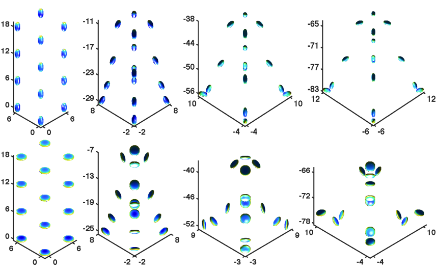
Figure 2: Sedimentation flow - regular lattice. Simulation of sedimentation for two lattices of ellipsoidal objects of equal weight. Color scheme corresponds to the magnitude of the total force field $||\rho_{i}+\mu_{i}||$. Top: snapshots for sedimentation of prolate ellipsoids, with semi-axes $(\frac{1}{2},\frac{1}{2},1)$. Bottom: snapshots for sedimentation of oblate ellipsoids, with semi-axes $(1,1,\frac{1}{3})$.

4.1.2 Low-Re swimmer models

One of the archetypal physical models to study swimming at low Reynolds numbers is the Najafi-Golestanian model [29], comprised of three aligned spheres connected by two arms. Because of the time-reversal symmetry of the Stokes equations, these arms must undergo a series of deformations asymmetric in time in order for the swimmer to locomote. The study and design of swimmers at small scales thus often relies on models that prescribe a series of strokes (displacements) for each arm between linked objects.

Alternatively, exploiting the linearity of the mobility problem (1.1), we opt for a model with periodic force and torque prescription for illustration purposes. The simplest instance consists of three aligned spheres with prescribed periodic, oscillating forces that sum to zero and no external torques:

$$\boldsymbol{[}F]_{1}(t)=(2\cos t+\sin t)\boldsymbol{[}e_{1}],\,\boldsymbol{[}F]_{2}(t)=(\sin t-\cos t)\boldsymbol{[}e_{1}],\ \boldsymbol{[}F]_{3}(t)=(-\cos t-2\sin t)\boldsymbol{[}e_{1}],\quad\left\{\boldsymbol{[}T]_{i}\right\}_{i=1}^{3}=\boldsymbol{[}0].$$ (4.2)

Due to the break in symmetry between the net forces for the two consecutive pairs of spheres, this arrangement has a net positive displacement on each time period $t\in[2\pi k,2\pi(k+1)]$. Since forces and torques are prescribed, setting up the BIE formulation and its numerical solution proceeds the same way as in Algorithm 1. We depict the self-locomotion of this 3-sphere swimmer in Figure 3. In addition, we use this model to test the convergence properties of our numerical algorithm in Section 4.3.

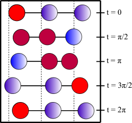
Figure 3: Force based 3-sphere swimmer. Motion of the 3-sphere swimmer with prescribed forces and torques given in (4.2). Spheres are colored on a linear gradient according to the force applied, with $F=2$ in red and $F=-2$ in blue. At the end of each cycle, the swimmer has a positive net displacement.

4.1.3 Magnetorheological fluid flows

A range of problems of interest in smart material design feature the study of colloidal suspensions which, when subjected to uniform magnetic fields [19] (or electric fields [11]), change their apparent viscosity and thus, their response to stress. These fluids are used in smart damping technology, with industrial, military and biomedical applications.

In order to study the rheology of these suspensions, especially at high concentration, a coupled system of evolution equations need to be solved to capture magnetic and hydrodynamic interactions. We assume the fluid to have zero susceptibility, and an absence of free currents. This allows us to represent the corresponding field as the negative gradient of a scalar potential $\phi$ and reduces the static Maxwell equations to a Laplace equation for $\phi$ with prescribed jump conditions at the particle boundaries. For example, for the magnetostatic case, the potential must satisfy the following equations:

$$\Delta\phi(\boldsymbol{[}x])=0\ \ \ \forall\,\boldsymbol{[}x]\notin\Gamma,$$ (4.3)

$$[[\phi]]_{\Gamma}=0,\ \ \ \left[\left[\mu\frac{\partial\phi}{\partial\boldsymbol{[}r]}\right]\right]_{\Gamma}=0,$$ (4.4)

$$\phi\rightarrow-\boldsymbol{[}H_{0}]\cdot\boldsymbol{[}r]\ \ \mathrm{as}\ \ |\boldsymbol{[}x]|\rightarrow\infty,$$ (4.5)

where $\mu$ is the magnetic permeability and $\boldsymbol{[}H]_{0}$ is the imposed magnetic field. We note that standard second-kind integral equation formulations exist for this problem [26]. If we represent $\phi=-\boldsymbol{[}H]_{0}\cdot\boldsymbol{[}x]+\mathcal{[}S]^{L}[q](\boldsymbol{[}x])$, where $\mathcal{[}S]^{L}$ is the Laplace single layer potential, $\mathcal{[}K]^{L}$ its normal derivative and $\eta=\frac{\mu-\mu_{0}}{\mu+\mu_{0}}$, enforcing the standard jump conditions [23] leads to the equation:

$$\left(\frac{1}{2}I+\eta\mathcal{[}K]^{L}_{\Gamma}\right)[q](x)=\eta\boldsymbol{[}H]_{0}\cdot\boldsymbol{[}n].$$ (4.6)

In order to couple Eq. (4.6) with our integral equation method for the fluid velocity, we recall that since the fluid medium is assumed to be insusceptible, the only interaction between them occurs through the traction force applied to the particle surfaces. For a given configuration of rigid bodies, we obtain the corresponding scalar potential $\phi$, and set the incident force field density $\rho_{i}$ to be the corresponding traction on surface $\Gamma_{i}$, which is computed using the Maxwell stress tensor.

We present a few characteristic examples of magnetorheological flow of suspensions of paramagnetic beads, following [19]. For two spherical beads, subjecting them to a uniform magnetic field $\boldsymbol{[}H]_{0}$ produces repulsive forces if $\boldsymbol{[}H]_{0}$ is perpendicular to the line that crosses their centers (see Fig. 4), and attractive forces if it is parallel. In the general case, it has been observed that particles tend to align, forming chains along the lines of magnetic field flux, as in Figures 1, 5 and 6.

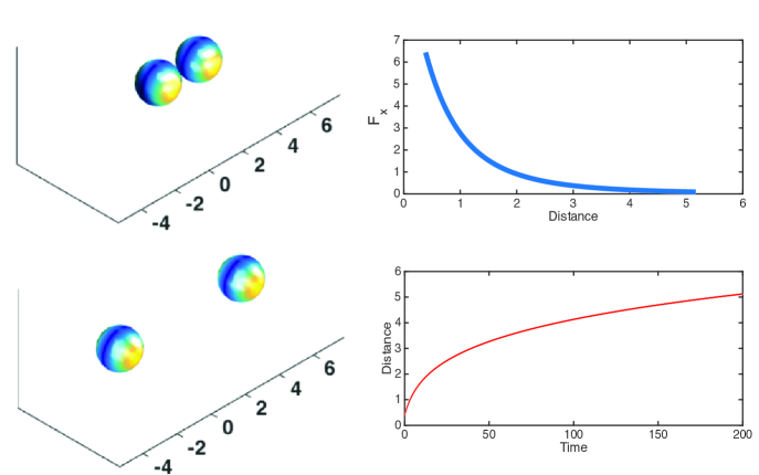
Figure 4: MHD flow - two sphere repulsion. Simulation of two spheres of radius $1$ in the x-axis, subjected to the uniform field $\boldsymbol{[}H]_{0}=(0,10,0)$, with $\mu/\mu_{0}=2$. Left: snapshots of simulation at $t=0$ and $t=200$. Color scheme is proportional to magnitude of incident force density $||\rho_{i}(x)||$. Top right: repulsion force magnitude as a function of sphere separation. Bottom right: separation as a function of time for $t\in[0,200]$.

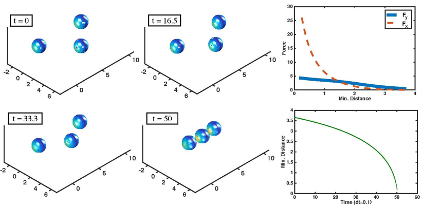
Figure 5: MHD flow - triangular configuration. Simulation of a triangular array of spheres of radius $1$, with centers $(0,0,0)$,$(0,8,0)$ and $(4,4,0)$ subjected to the uniform field $\boldsymbol{[}H]_{0}=(0,10,0)$, with $\mu/\mu_{0}=2$. Top: snapshots at $t=0,16.5,33.3$ and $t=50$. Spheres are colored according to the magnitude of incident force density $||\rho_{i}(x)||$. Bottom left: attractive force magnitude in $x$ and $y$ as a function of minimum sphere separation. Bottom right: separation as a function of time $t\in[0,50]$.

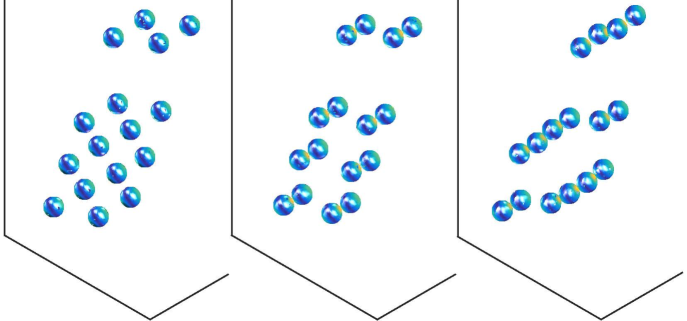
Figure 6: MHD flow - chain formation. Simulation of spheres of radius $1$ with centers on a perturbed lattice, subjected to the uniform field $\boldsymbol{[}H]_{0}=\frac{10}{\sqrt{3}}(1,-1,-1)$, with $\mu/\mu_{0}=2$. Spheres are colored according to the magnitude of incident force density $||\rho_{i}(x)||$. Left: initial configuration. Middle: pairs form among closest spheres. Right: pairs begin to coalesce into larger chains, aligned with the magnetic field.

4.2 Scaling tests

In order to test experimental scaling for the computational costs of our method, we set a sedimentation simulation with an initial configuration of $2\times 2\times n_{z}$ spheres of radius $1$ on a regular lattice with center spacing equal to $5$. We then evolve the system for $100$ timesteps and record the average time our solver takes per timestep. We test scaling with respect to the number of objects $n=4n_{z}$ for $n=\{32,64,128\}$ as well as the order $p$ of spherical harmonic approximations by comparing results for $p=8$ and $p=16$. All tests are performed serially on Intel Xeon E–$2690$ v$2$($3.0$ GHz) nodes with $24$ GB of memory.

$n$	$p=8$		$p=16$
	$\centering N\@add@centering$	Time (sec)	$\centering N\@add@centering$	Time (sec)
$\centering 32\@add@centering$	$\centering 13824\@add@centering$	$\centering 12.88\@add@centering$	$\centering 52224\@add@centering$	$\centering 132.3\@add@centering$
$\centering 64\@add@centering$	$\centering 27648\@add@centering$	$\centering 24.97\@add@centering$	$\centering 104448\@add@centering$	$\centering 272.4\@add@centering$
$\centering 128\@add@centering$	$\centering 55296\@add@centering$	$\centering 49.49\@add@centering$	$\centering 208896\@add@centering$	$\centering 544.2\@add@centering$

Table 1: Sphere lattice total per timestep. Average timings (in seconds) per timestep for the evolution under gravity of a $2\times 2\times n_{z}$ regular lattice of spheres of radius $1$ and spacing $5$.

Theoretical scaling for the matrix apply is $\mathscr{O}\left(n(p^{4}+p^{2})\right)$, since it involves the computation of self-interactions (dense apply of $n$ matrices of size $6p(p+1)\times 6p(p+1)$) and one particle Stokes FMM, which is $\mathscr{O}\left(N\right)=\mathscr{O}\left(p^{2}n\right)$. As we observe in our profiling, computational cost per timestep is largely dominated by the solution of the integral equation for the scattered field density (using GMRES). Hence, the experimental scaling observed matches that of the fast matrix apply: we observe linear scaling with respect to $n$, and doubling $p$ increases the cost by a factor of $11$ for the cases observed.

Profiling

For each of the experiments described above, we measure average timings for the steps in Algorithm 1: incident field density computation (line 3), scattered field density solve (line 4), rigid body velocity evaluation (line 5), collision detection (line 7), and operator update (line 11 - 12).

We observe that computational cost is largely dominated by the solve, taking up about $80\%$ of the total time per timestep. It takes $4$-$5$ iterations for the preconditioned GMRES to reach target accuracy, which we set at $10^{-6}$. We note that iteration counts and average solve times, while largely independent of $n$ and $p$, tend to increase in cases where surfaces come close to contact. This may be addressed by the use of more adequate preconditioners (such as sparse approximate inverse (SPAI), multilgrid or low accuracy direct solvers).

In the operator update stage, we update self-interaction matrices as well as the block-diagonal preconditioner to match the new center positions and rotation matrices. This stage takes up $10$-$15\%$ of the total time. The cost of evaluating $\boldsymbol{[}u]$ and computing rigid body velocities is essentially that of a fast matrix-vector apply, accounts for most of the remaining timings observed.

$n$	$p=8$					$p=16$
	$\centering N\@add@centering$	Apply (sec)	Solve (sec)	Update (sec)		$\centering N\@add@centering$	Apply (sec)	Solve (sec)	Update (sec)
$\centering 32\@add@centering$	$\centering 13824\@add@centering$	$\centering 1.09\@add@centering$	$\centering 10.25\@add@centering$	$\centering 1.53\@add@centering$		$\centering 52224\@add@centering$	$\centering 10.7\@add@centering$	$\centering 108.9\@add@centering$	$\centering 12.65\@add@centering$
$\centering 64\@add@centering$	$\centering 27648\@add@centering$	$\centering 2.26\@add@centering$	$\centering 19.51\@add@centering$	$\centering 3.19\@add@centering$		$\centering 104448\@add@centering$	$\centering 21.5\@add@centering$	$\centering 220.3\@add@centering$	$\centering 30.49\@add@centering$
$\centering 128\@add@centering$	$\centering 55296\@add@centering$	$\centering 4.75\@add@centering$	$\centering 38.41\@add@centering$	$\centering 6.30\@add@centering$		$\centering 208896\@add@centering$	$\centering 42.9\@add@centering$	$\centering 439.9\@add@centering$	$\centering 61.18\@add@centering$

Table 2: Sphere lattice profile per timestep. Average timings (in seconds) per timestep for scattered field density solve and operator updates. Matrix-vector apply time is included to account for velocity evaluation, as well as for comparison with the GMRES solve. Incident field density computation is negligible, and no contact force correction was necessary for the experiments presented.

The same set of tests were ran for regular lattices of ellipsoids with semi-axes $(a,b,c)=(1,0.5,0.5)$ and $(a,b,c)=(1,1,0.5)$. We note that, while showing a slight increase in the solve stage (corresponding to iteration counts of $5$-$6$ iterations for the preconditioned GMRES), their performance in terms of scaling and profiling was similar to that presented above.

4.3 Convergence tests

In order to test convergence of our method with respect to the integral operator discretization (controlled by the order $p$ of the spherical harmonic appproximation) and the proposed time-stepping schemes, we set a series of experiments for a swimmer comprised either of three spheres or of three ellipsoids with the same proportions. We apply periodic, oscillatory forces in the $x$-axis, as well as oscillatory torques along the $y$-axis.

$$\boldsymbol{[}F]_{1}(t)=(2\cos t+\sin t)\boldsymbol{[}e_{1}],\ \boldsymbol{[}F]_{2}(t)=(\sin t-\cos t)\boldsymbol{[}e_{1}],\ \boldsymbol{[}F]_{3}(t)=(-\cos t-2\sin t)\boldsymbol{[}e_{1}]$$

$$\boldsymbol{[}T]_{1}(t)=(2\cos t+\sin t)\boldsymbol{[}e_{2}],\ \boldsymbol{[}T]_{2}(t)=(\sin t-\cos t)\boldsymbol{[}e_{2}],\ \boldsymbol{[}T]_{3}(t)=(-\cos t-2\sin t)\boldsymbol{[}e_{2}]$$

These modifications to the standard swimmer allow us to test convergence of both centers and rotation matrices, for both spherical and non-spherical shapes. At the end of each cycle of size $2\pi$, the three object swimmer displays net positive displacement along the $x$-axis, as well as slight displacements in the $z$-axis.

Spatial discretization

We evolve one three-object swimmer for a full cycle $t\in[0,2\pi]$, for $p\in\{2,4,8,16\}$, using a forward euler time-stepping scheme with $\Delta t=\frac{2\pi}{128}$. At the final time $T=2\pi$, we test self-convergence of the rigid object centers and rotations by measuring the following quantities:

$$\mathcal{E}_{C}(T,p)=-\log_{2}\underset{i\leq 3}{max}||C_{i}^{p}(T)-C_{i}^{2p}(T)||_{2}$$

$$\mathcal{E}_{R}(T,p)=-\log_{2}\underset{i\leq 3}{max}||R_{i}^{p}(T)-R_{i}^{2p}(T)||_{F}$$

We compare results for spheres and ellipsoids with semi-axes $(a,a,1)$ for $a=\frac{1}{2},\frac{1}{4}$.

		$p=2$	$p=4$	$p=8$
Sphere	$\centering\mathcal{E}_{C}(T,p)\@add@centering$	$\centering 5.67\@add@centering$	$\centering 14.86\@add@centering$	$\centering 29.98\@add@centering$
	$\centering\mathcal{E}_{M}(T,p)\@add@centering$	$\centering 9.31\@add@centering$	$\centering 15.19\@add@centering$	$\centering 29.93\@add@centering$
Ellipsoid $\frac{1}{2}$	$\centering\mathcal{E}_{C}(T,p)\@add@centering$	$\centering 3.76\@add@centering$	$\centering 7.12\@add@centering$	$\centering 13.96\@add@centering$
	$\centering\mathcal{E}_{M}(T,p)\@add@centering$	$\centering 5.13\@add@centering$	$\centering 9.77\@add@centering$	$\centering 15.82\@add@centering$
Ellipsoid $\frac{1}{4}$	$\centering\mathcal{E}_{C}(T,p)\@add@centering$	$\centering-\@add@centering$	$\centering 7.53\@add@centering$	$\centering 10.83\@add@centering$
	$\centering\mathcal{E}_{M}(T,p)\@add@centering$	$\centering-\@add@centering$	$\centering 7.98\@add@centering$	$\centering 10.95\@add@centering$

Table 3: Spatial discretization self-convergence. Error terms for center and rotation matrix evolution of three-object swimmers at final time $T=2\pi$ for for $p\in\{2,4,8,16\}$.

For both center and rotation matrix evolution we compare the columns in Table 3 and observe that the convergence rate is proportional to $p$. This is in accordance with the theoretical spectral convergence of the quadrature rules employed. We note that, as we increase surface complexity (in this case dependent on the eccentricity of the ellipsoids), the approximation order $p$ required to reach a certain target accuracy increases.

Time discretization

We test the rate of convergence with respect to $\Delta t$ of our proposed time-stepping scheme for trapezoidal and Runge-Kutta 4 methods. We again evolve a three-object swimmer for a full cycle $t\in[0,2\pi]$, for $p=8$ and $\Delta t=2\pi/\{16,32,\dots,256\}$. At the final time $T=2\pi$, we measure the following quantities:

$$\mathcal{E}_{C}(T,\Delta t)=-\log_{2}\underset{i\leq 3}{max}||C_{i}^{\Delta t}(T)-C_{i}^{\Delta t/2}(T)||_{2}$$

$$\mathcal{E}_{R}(T,\Delta t)=-\log_{2}\underset{i\leq 3}{max}||R_{i}^{\Delta t}(T)-R_{i}^{\Delta t/2}(T)||_{F}$$

		$\Delta t=\frac{2\pi}{16}$	$\Delta t=\frac{2\pi}{32}$	$\Delta t=\frac{2\pi}{64}$	$\Delta t=\frac{2\pi}{128}$
Sphere	$\centering\mathcal{E}_{C}(T,\Delta t)\@add@centering$	$\centering 8.61\@add@centering$	$\centering 11.59\@add@centering$	$\centering 14.21\@add@centering$	$\centering 16.67\@add@centering$
	$\centering\mathcal{E}_{M}(T,\Delta t)\@add@centering$	$\centering 6.26\@add@centering$	$\centering 8.80\@add@centering$	$\centering 11.15\@add@centering$	$\centering 13.16\@add@centering$
Ellipsoid $\frac{1}{2}$	$\centering\mathcal{E}_{C}(T,\Delta t)\@add@centering$	$\centering 9.63\@add@centering$	$\centering 11.98\@add@centering$	$\centering 14.20\@add@centering$	$\centering 15.99\@add@centering$
	$\centering\mathcal{E}_{M}(T,\Delta t)\@add@centering$	$\centering 7.87\@add@centering$	$\centering 9.87\@add@centering$	$\centering 11.87\@add@centering$	$\centering 13.86\@add@centering$
Ellipsoid $\frac{1}{4}$	$\centering\mathcal{E}_{C}(T,\Delta t)\@add@centering$	$\centering 7.17\@add@centering$	$\centering 9.77\@add@centering$	$\centering 12.25\@add@centering$	$\centering 14.58\@add@centering$
	$\centering\mathcal{E}_{M}(T,\Delta t)\@add@centering$	$\centering 5.36\@add@centering$	$\centering 7.85\@add@centering$	$\centering 10.26\@add@centering$	$\centering 12.52\@add@centering$

Table 4: Trapezoidal method self-convergence. Error terms for center and rotation matrix evolution of three-object swimmers at final time $T=2\pi$ for the trapezoidal method, for $p=8$ and $\Delta t\in\{\frac{2\pi}{16},\frac{2\pi}{32},\frac{2\pi}{64},\frac{2\pi}{128}\}$.

		$\Delta t=\frac{2\pi}{16}$	$\Delta t=\frac{2\pi}{32}$	$\Delta t=\frac{2\pi}{64}$	$\Delta t=\frac{2\pi}{128}$
Sphere	$\centering\mathcal{E}_{C}(T,\Delta t)\@add@centering$	$\centering 19.75\@add@centering$	$\centering 23.77\@add@centering$	$\centering 27.78\@add@centering$	$\centering 31.80\@add@centering$
	$\centering\mathcal{E}_{M}(T,\Delta t)\@add@centering$	$\centering 21.49\@add@centering$	$\centering 25.50\@add@centering$	$\centering 29.51\@add@centering$	$\centering 33.50\@add@centering$
Ellipsoid $\frac{1}{2}$	$\centering\mathcal{E}_{C}(T,\Delta t)\@add@centering$	$\centering 18.32\@add@centering$	$\centering 22.33\@add@centering$	$\centering 26.34\@add@centering$	$\centering 30.34\@add@centering$
	$\centering\mathcal{E}_{M}(T,\Delta t)\@add@centering$	$\centering 18.48\@add@centering$	$\centering 22.49\@add@centering$	$\centering 26.51\@add@centering$	$\centering 30.52\@add@centering$
Ellipsoid $\frac{1}{4}$	$\centering\mathcal{E}_{C}(T,\Delta t)\@add@centering$	$\centering 17.01\@add@centering$	$\centering 21.01\@add@centering$	$\centering 25.02\@add@centering$	$\centering 29.01\@add@centering$
	$\centering\mathcal{E}_{M}(T,\Delta t)\@add@centering$	$\centering 16.94\@add@centering$	$\centering 21.00\@add@centering$	$\centering 25.03\@add@centering$	$\centering 29.06\@add@centering$

Table 5: Runge-Kutta 4 method self-convergence. Error terms for center and rotation matrix evolution of three-object swimmers at final time $T=2\pi$ for the explicit Runge-Kutta method of order $4$, for $p=8$ and $\Delta t\in\{\frac{2\pi}{16},\frac{2\pi}{32},\frac{2\pi}{64},\frac{2\pi}{128}\}$.

By comparing the columns in Table 4 and Table 5, we confirm that for both center and rotation matrix evolution, the proposed explicit Runge-Kutta time-stepping schemes display second and fourth order convergence, respectively.

5 Conclusions

We presented a new BIE formulation for the mobility problem in three dimensions. Its main advantages are that auxiliary sources inside each rigid body—required by classical approaches such as the completed double-layer formulation [33]—are obviated, thereby reducing the number of unknowns, and that hypersingular integrals are avoided when computing the hydrodynamic stresses. The extra linear conditions in the case of the scattered field problem i.e., zero net force and torque constraints on the particles, are imposed by simply modifying the BIEs for the densities. Unlike classical formulations, the translational and rotational velocities of each particle are not the fundamental variables but are determined by integrating the surface velocities of each particle.

The numerical method proposed is spectrally-accurate in space via the use of spherical harmonics to represent the geometries and densities and a pole-rotation based singular integration scheme. We couple Stokes FMM with a preconditioned GMRES solver to obtain a solution method that scales linearly with the number of particles. A fourth-order explicit Runge-Kutta method was then used to evolve the particle positions. We presented a series of numerical results that verified the convergence and scaling analysis of our method.

The mobility problem arises naturally in many physical models, and we demonstrated the applicability of our solution process to sedimentation problems, low-Re swimmer models and magneto-rheological fluid models. The method naturally extends to another important setting, that of when a background flow is imposed. It can be in the form of free-space velocity field i.e., $\boldsymbol{[}u](\boldsymbol{[}x])\rightarrow\boldsymbol{[}u]_{\infty}(\boldsymbol{[}x])\ \ \mathrm{as}\ \ |\boldsymbol{[}x]|\rightarrow\infty$, or disturbance velocity field in the case of flows through constrained geometries. In both cases, due to the linearity of Stokes flow, the imposed field simply is added to the boundary integral representation of the scattered field e.g., $\boldsymbol{[}u]_{sc}=\boldsymbol{[}u]_{\infty}+\mathcal{[}S]_{\Gamma}[\boldsymbol{[}\mu]]$. The BIEs are then modified accordingly.

Robust simulation of dense particle suspensions requires several more algorithmic components. When the particles are located close to each other, the interaction terms become nearly singular and specialized quadratures are required to achieve uniform high-order convergence. We plan to extend the recently developed quadrature-by-expansion (QBX) [21] to three dimensions. While the recent work of [20] implemented a QBX method for three-dimensional problems, the particle shapes were restricted to spheroids. Adaptive time-stepping also becomes important to resolve close interactions. Finally, to enable simulations through periodic geometries, we plan to extend the recently developed periodization scheme in [27] to the mobility problem. This scheme uses free-space kernels only and the FMM can be used to accelerate the discrete sums as we do in this work.

6 Acknowledgements

EC and SV acknowledge support from NSF under grants DMS-1224656, DMS-1454010 and DMS-1418964 and a Simons Collaboration Grant for Mathematicians #317933. LG and MR acknowledge support from the U.S. Department of Energy Office of Science, Office of Advanced Scientific Computing Research, Applied Mathematics program under Award Number DEFGO288ER25053 and the Office of the Assistant Secretary of Defense for Research and Engineering and AFOSR under NSSEFF Program Award FA9550-10-1-0180.

References

• Af Klinteberg and Tornberg [2014] Ludvig Af Klinteberg and Anna-Karin Tornberg. Fast Ewald summation for Stokesian particle suspensions. International Journal for Numerical Methods in Fluids, 76(10):669–698, 2014.
• Barnett et al. [2015] Alex Barnett, Bowei Wu, and Shravan Veerapaneni. Spectrally accurate quadratures for evaluation of layer potentials close to the boundary for the 2d stokes and laplace equations. SIAM Journal on Scientific Computing, 37(4):B519–B542, 2015.
• Beale and Lai [2001] J Thomas Beale and Ming-Chih Lai. A method for computing nearly singular integrals. SIAM Journal on Numerical Analysis, 38(6):1902–1925, 2001.
• Bebendorf [2005] Mario Bebendorf. Hierarchical lu decomposition-based preconditioners for bem. Computing, 74(3):225–247, 2005.
• Boyd [2001] John P Boyd. Chebyshev and Fourier spectral methods. Courier Corporation, 2001.
• Chew et al. [2001] W. C. Chew, J.-M. Jin, E. Michielssen, and J. Song. Fast and Efficient Algorithms in Computational Electromagnetics. Artech House, Boston, 2001.
• Corona et al. [2014] E. Corona, P.G. Martinsson, and D. Zorin. An O(N) direct solver for integral equations on the plane. Applied and Computational Harmonic Analysis, 2014.
• Corona et al. [2015] E. Corona, A. Rahimian, and D. Zorin. A tensor-train accelerated solver for integral equations in complex geometries. arXiv preprint arXiv:1511.06029, 2015.
• Cortez et al. [2005] Ricardo Cortez, Lisa Fauci, and Alexei Medovikov. The method of regularized Stokeslets in three dimensions: Analysis, validation, and application to helical swimming. Physics of Fluids, 17(3):031504, 2005.
• Coulier et al. [2015] Pieter Coulier, Hadi Pouransari, and Eric Darve. The inverse fast multipole method: using a fast approximate direct solver as a preconditioner for dense linear systems. arXiv preprint arXiv:1508.01835, 2015.
• Das and Saintillan [2013] Debasish Das and David Saintillan. Electrohydrodynamic interaction of spherical particles under quincke rotation. Physical Review E, 87(4):043014, 2013.
• Gimbutas and Greengard [2012] Zydrunas Gimbutas and Leslie Greengard. FMMLIB3D 1.2, 2012. URL http://www.cims.nyu.edu/cmcl/fmm3dlib/fmm3dlib.html.
• Gimbutas and Veerapaneni [2013] Zydrunas Gimbutas and Shravan Veerapaneni. A fast algorithm for spherical grid rotations and its application to singular quadrature. SIAM Journal on Scientific Computing, 35(6):A2738–A2751, 2013.
• Golestanian and Ajdari [2008] Ramin Golestanian and Armand Ajdari. Analytic results for the three-sphere swimmer at low reynolds number. Physical Review E, 77(3):036308, 2008.
• Greengard and Rokhlin [1997] L. Greengard and V. Rokhlin. A new version of the fast multipole method for the Laplace equation in three dimensions. In Acta numerica, 1997, volume 6 of Acta Numer., pages 229–269. Cambridge Univ. Press, Cambridge, 1997.
• Helsing and Ojala [2008] Johan Helsing and Rikard Ojala. On the evaluation of layer potentials close to their sources. Journal of Computational Physics, 227(5):2899–2921, 2008.
• Ho and Ying [2013] K. Ho and L. Ying. Hierarchical interpolative factorization for elliptic operators: integral equations. arXiv preprint arXiv:1307.2666, 2013.
• Karrila and Kim [1989] Seppo J Karrila and Sangtae Kim. Integral equations of the second kind for Stokes flow: direct solution for physical variables and removal of inherent accuracy limitations. Chemical engineering communications, 82(1):123–161, 1989.
• Keaveny and Maxey [2008] Eric E Keaveny and Martin R Maxey. Modeling the magnetic interactions between paramagnetic beads in magnetorheological fluids. Journal of Computational Physics, 227(22):9554–9571, 2008.
• Klinteberg and Tornberg [2016] Ludvig af Klinteberg and Anna-Karin Tornberg. A fast integral equation method for solid particles in viscous flow using quadrature by expansion. arXiv preprint arXiv:1604.07186, 2016.
• Klöckner et al. [2013a] A. Klöckner, A. Barnett, L. Greengard, and M. OʼNeil. Quadrature by expansion: a new method for the evaluation of layer potentials. Journal of Computational Physics, 252:332–349, 2013a.
• Klöckner et al. [2013b] Andreas Klöckner, Alexander Barnett, Leslie Greengard, and Michael O?Neil. Quadrature by expansion: A new method for the evaluation of layer potentials. Journal of Computational Physics, 252:332–349, 2013b.
• Kress et al. [1989] Rainer Kress, V Maz’ya, and V Kozlov. Linear integral equations, volume 82. Springer, 1989.
• Kropinski [1999] Mary Catherine Kropinski. Integral equation methods for particle simulations in creeping flows. Computers & Mathematics with Applications, 38(5-6):67–87, September 1999. ISSN 08981221. doi: 10.1016/S0898-1221(99)00215-1.
• Liu [2009] Y. Liu. Fast Multipole Boundary Element Method: Theory and Applications in Engineering. Cambridge University Press, New York, 2009.
• Ly et al. [1999] HV Ly, F Reitich, MR Jolly, Harvey Thomas Banks, and Kazi Ito. Simulations of particle dynamics in magnetorheological fluids. Journal of Computational Physics, 155(1):160–177, 1999.
• Marple et al. [2015] Gary Marple, Alex Barnett, Adrianna Gillman, and Shravan Veerapaneni. A fast algorithm for simulating multiphase flows through periodic geometries of arbitrary shape. arXiv preprint arXiv:1510.05616, 2015.
• Mohlenkamp [1999] Martin J Mohlenkamp. A fast transform for spherical harmonics. Journal of Fourier analysis and applications, 5(2-3):159–184, 1999.
• Najafi and Golestanian [2004] Ali Najafi and Ramin Golestanian. Simple swimmer at low reynolds number: Three linked spheres. Physical Review E, 69(6):062901, 2004.
• Nishimura [2002] N. Nishimura. Fast multipole accelerated boundary integral equation methods. Appl. Mech. Rev., 55:299–324, 2002.
• Ojala and Tornberg [2015] Rikard Ojala and Anna-Karin Tornberg. An accurate integral equation method for simulating multi-phase stokes flow. Journal of Computational Physics, 298:145–160, 2015.
• Orszag [1974] Steven A Orszag. Fourier series on spheres. Monthly Weather Review, 102(1):56–75, 1974.
• Pozrikidis [1992] C. Pozrikidis. Boundary Integral and Singularity Methods for Linearized Viscous Flow. Cambridge Texts in Applied Mathematics. Cambridge University Press, 1992. ISBN 9780521406932.
• Quaife and Biros [2014] Bryan Quaife and George Biros. High-volume fraction simulations of two-dimensional vesicle suspensions. Journal of Computational Physics, 274:245–267, 2014.
• Quaife and Biros [2015] Bryan Quaife and George Biros. On preconditioners for the laplace double-layer in 2d. Numerical Linear Algebra with Applications, 22(1):101–122, 2015.
• Rachh [2015] Manas Rachh. Integral equation methods for problems in electrostatics, elastostatics and viscous flow. 2015. Thesis (Ph.D.)–New York University.
• Rachh and Greengard [2015] Manas Rachh and Leslie Greengard. Integral equation methods for elastance and mobility problems in two dimensions. arXiv preprint arXiv:1507.05925, 2015.
• Saad and Schultz [1986] Y. Saad and M.H. Schultz. GMRES: A generalized minimal residual algorithm for solving nonsymmetric linear systems. SIAM Journal on Scientific and Statistical Computing, 7(3):856–869, 1986.
• Tlupova and Beale [2013] Svetlana Tlupova and J Thomas Beale. Nearly singular integrals in 3d stokes flow. Communications in Computational Physics, 14(05):1207–1227, 2013.
• Vavasis [1992] Stephen A Vavasis. Preconditioning for boundary integral equations. SIAM journal on matrix analysis and applications, 13(3):905–925, 1992.
• Veerapaneni et al. [2011] Shravan K Veerapaneni, Abtin Rahimian, George Biros, and Denis Zorin. A fast algorithm for simulating vesicle flows in three dimensions. Journal of Computational Physics, 230(14):5610–5634, 2011.
• Ying et al. [2004] L. Ying, G. Biros, and D. Zorin. A kernel independent adaptive fast multipole algorithm in two and three dimensions. Journal of Computational Physics, 196(2):591–626, 2004.
• Ying et al. [2006] Lexing Ying, George Biros, and Denis Zorin. A high-order 3d boundary integral equation solver for elliptic pdes in smooth domains. Journal of Computational Physics, 219(1):247–275, 2006.