Deep XMM-Newton Observations of the NW Radio Relic Region of Abell 3667

Abstract

The results of long XMM-Newton X-ray observations of the NW radio relic of Abell 3667 are presented. A shock is detected at the sharp outer edge of the radio relic, both in the X-ray surface brightness and the temperature profiles. The Mach number is ${\cal{M}}=2.54^{+0.80}_{-0.43}$. The temperature jump at the shock is larger than expected from the density jump, which may indicate that a dynamically important magnetic field aligned primarily parallel to the shock front is present. The gas temperature rises gradually over several arc minutes within the shock region. This could indicate that the shock energy is initially dissipated into some mix of thermal and nonthermal (e.g., turbulence) components, and that the nonthermal energy decays into heat in the post-shock region. The observed radio relic can be powered if $\sim$0.2% of the energy dissipated in the shock goes into the (re)acceleration of relativistic electrons. We show that the observed steepening of the radio spectrum with distance behind the shock is consistent with radiative losses by the radio-emitting electrons. However, the radio spectrum immediately behind the shock is flatter than expected for linear diffusive shock acceleration of thermal electrons. This suggests that the shock re-accelerates a pre-existing population of relativistic electrons. We also detect a bright, cool region (the “Mushroom”) to the south of the radio relic, which we propose is the remnant cool core of a merging subcluster, and that this subcluster was the driver for the observed NW shock. In this model, the properties of Abell 3667 are mainly the result of an offset binary merger, and the cluster is being observed about 1 Gyr after first core passage. We predict that deeper X-ray or SZ observations of the SE radio relic will reveal a second merger shock at the outer edge.

1. Introduction

Clusters of galaxies are the largest relaxed systems in the Universe. They form hierarchically by the merger of smaller systems. While the most common mergers involve relatively small groups or even individual galaxies, major cluster mergers of similar-sized subclusters also occur with a significant frequency. These major cluster mergers are probably the most energetic events which have occurred in the Universe since the Big Bang. They drive shocks into the intracluster medium of the subclusters. Although most merger shocks have relatively low Mach numbers of ${\cal{M}}\approx 1$–3, shocks are the most important source of heating for the intracluster medium in massive clusters.

Most collisionless astrophysical shocks in low density gas also accelerate electrons (and presumably, ions) to relativistic energies. In fact, extended diffuse cluster radio sources with steep spectra and no clear optical counterparts have been known for over 40 years (Willson 1970; Feretti et al. 2012). They have such steep radio spectra that in most cases they can be detected only at lower frequencies ($\lesssim$5 GHz). Sources which are relatively symmetric and are projected on the cluster center are often referred to as “radio halos” (e.g., Deiss et al. 1997), while elongated sources usually located on the cluster periphery are called “relics.” In essentially every case, these diffuse cluster radio sources have been found in irregular clusters that are undergoing mergers. This suggests that the radio emitting electrons are accelerated or re-accelerated by some merger-driven process. One possible theoretical picture is that halos are due to relativistic electrons (re)accelerated by turbulence behind merger shocks, while the relics are the direct result of merger shock acceleration (e.g., Feretti et al. 2012). If the relics are due to shock acceleration, then there should be a merger shock with its associated temperature and density jump at one edge (generally the outer edge) of the relic, and the relic radio spectrum should be flatter there due to recent acceleration. On the other hand, if a relic is due to adiabatic compression of a pre-existing radio lobe, any merger shock will likely be beyond the relic, and no clear radio spectral variation is expected.

Abell 3667 is a violently merging, relatively low redshift $(z=0.05525$) cluster (Markevitch et al. 1999). Early Chandra observations detected a merger cold front near the center (Vikhlinin et al. 2001b, a), and the term “cold front” was coined based in part on the Abell 3667 observations. Subsequent Chandra and XMM/Newton observations (Mazzotta et al. 2002; Briel et al. 2004) provided spectacularly detailed images and information on the dynamics of the merger, but were mainly concentrated on the interior regions, not the outer regions near the radio relics.

Abell 3667 contains a pair of curved cluster radio relics (Röttgering et al. 1997), which are located on either side of the cluster center at large radii. Their locations and sharp, inwardly curved outer edges are consistent with particle acceleration by merger shocks. In this picture, the shocks would be located at the outer edges of the two relics. The northwest radio relic in Abell 3667 is the brightest cluster radio relic or halo source which is known, with a flux at 20 cm of 3.7 Jy (Johnston-Hollitt 2004). It is also one of the largest relics, with a total extent of 33′ or 2.1 Mpc. Its radio spectrum steepens with distance from the outer edge (Röttgering et al. 1997) as expected if the electrons are accelerated there and the higher energy electrons lose energy due to synchrotron and IC emission as they are advected away from the shock.

Roettiger et al. (1999) presented a numerical MHD/N-body simulation of Abell 3667 with parameters chosen to match crudely the observed properties of the cluster. In their model, Abell 3667 is an offset binary merger which is currently $\sim$1 Gyr beyond first core passage. The mass ratio in their model was 5:1. The smaller subcluster merged from the SE, and has driven a shock ahead of it which corresponds in position to the NW radio relic. A second shock was driven by the primary cluster, and is at the location of the SE radio relic. There were also a few weaker and smaller shocks near the center of the cluster without clear radio counterparts. More recently, Datta et al. (2014) presented a more complicated MHD/N-body simulation with initial conditions drawn from a cosmological simulation. This simulation was not tuned to represent Abell 3667 specifically, but does show many of the same features as the Roettiger et al. (1999) simulation.

Recently, diffuse radio emission has been detected near the center of Abell 3667. Parkes and Australia Telescope Compact Array observations show an unpolarized radio “bridge” running from the NW radio relic to the center of the cluster (Carretti et al. 2013). They argue that this bridge is a turbulent wake associated with a merging subcluster and the merger shock which made the NW radio relic. Observations with the Karoo Array Telescope (KAT-7) don’t detect the bridge, but do find a possible radio mini-halo associated with the brightest cluster galaxy, B2007$-$569 (Riseley et al. 2015).

Here, we present the results of a series of long XMM-Newton observations of Abell 3667 which cover the region of the NW radio relic. The X-ray observations and data analysis are described in § 2. The X-ray images and surface brightness profiles are given in § 3. In § 4, the X-ray spectra and cluster temperature map are presented. We discuss the implications of these observations in § 5. Our conclusions are summarized in § 6. Appendices give the expressions used to model shocks observed in the X-ray image. We assume a $\Lambda$CDM cosmology with $H_{0}=71$ km s^-1 Mpc^-1, $\Omega_{M}=0.27$, and $\Omega_{\lambda}=0.73$. At the redshift of Abell 3667 of $z=0.05525$, the angular diameter distance is $d_{A}=212.6$ Mpc, and 1′ corresponds to 61.8 kpc. For a mean cluster temperature of 7.2 keV, the virial radius should be $r_{180}\approx 2.33$ Mpc $=38\arcmin$ (Markevitch et al. 1998). (Within the radius $r_{180}$, the average density is 180 times the cosmological critical density at the cluster redshift.) Unless otherwise specified, we provide confidence intervals at the 68% level.

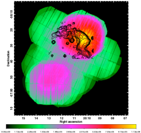
Figure 1.— The exposure map showing the total amount of good time for all of the images and all of the observations of Abell 3667. The color bar at the bottom shows the total exposure in seconds with a square-root scaling. The SUMSS 843 MHz radio contours from the region of the NW radio relic are shown black (8 countours logarithmically distributed between 1 and 23 mJy beam^-1).

2. X-ray Observation and Data Reduction

The eight previous XMM-Newton observations of Abell 3667 were discussed in Finoguenov et al. (2010, hereafter FSN); six of these observations, which concentrate on the center of the cluster, were analyzed in Briel et al. (2004). We observed the northwest region of the cluster, including the area of the NW radio relic, with XMM-Newton in orbit 1620 (OBSID 0553180101). Based on the results from this observation, we proposed a much longer observation of the NW region of the cluster, which was done on 2010 September 21–27, October 3, November 2–3. There were four pointings centered on the NW radio relic (OBSIDs 065305401, 065305501, 065305601, and 065305601 in orbits 1976–1978 and 1996) for a total of 290 ksec, and two pointings on either side (east and west) of the relic (OBSIDs 065305201 and 065305301 in orbits 1975 and 1981) of 30.0 and 26.0 ksec. The medium filter has been used for all instruments for consistency with the previous observations of the cluster. The observations were done in extended full frame mode for the pn to reduce the effect of out-of-time events. We checked whether any of the CCDs were in anomalous states with unusually high background, and removed CCD4 of MOS1 from observations 0553180101, 0653050301, 0653050401, 0653050501 and CCD5 of MOS2 from 0553180101.

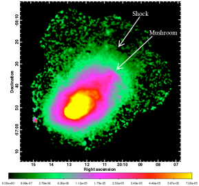
Figure 2.— X-ray mosaic image from XMM-Newton in the 0.5–2.0 keV band (excluding the instrumental Al line at $\sim$1.5 keV). the image has been corrected for exposure and background, and all point sources have been removed from the image. Left: XMM image with NW features labelled. Right: XMM image with SUMSS 843 MHz radio contours shown.

We used sas version 13.5.0 for the standard data reduction. After producing the event files, we have applied a strict light curve cleaning (e.g., Zhang et al. 2004) in order to ensure that we retained only the periods with the lowest and the most stable background. The new data was combined with all of the previous observations to make a mosaic. Figure 1 gives the total exposure maps showing the total of all of the good time for all of the observations and for the sum of MOS1, MOS2, and pn detectors. The maximum total exposure, in the center of the NW Radio Relic, is $1.13\times 10^{6}$ sec.

The quadruple background subtraction technique of Finoguenov et al. (2007) was used to model the background, and remove it from the images and surface brightness profiles.

The point sources in the X-ray mosaic were detected, modeled using the XMM PSF, and subtracted from the images and surface brightness profiles described below. For the spectral analysis, we excised the regions where contribution from point source emission could be significant, and in a similar way we excised the detected point sources in the background file, so remaining emission from the wings of PSF which is confused, is subtracted by using the background file.

The instrumental background level at the epoch of latest Abell 3667 observations was substantially higher than the background level typical for the publicly available calibration products and the quality of the background subtraction was not satisfactory. To remedy the problem, we have used the XMM observations of the Chandra Deep Field South (CDFS) field (Comastri et al. 2011; Finoguenov et al. 2015), which were performed at a similar epoch to A3667 observations. We have chosen with work with the pn detector, for which we have confidence in our knowledge of the instrumental characteristics. We collected 265 ksec of cleaned data of the CDFS observations performed in 2010 and masked out the areas where strong point sources were present. The different choice of filters for the CDFS observations precludes using energies below 0.8 keV in the spectral analysis, so we have concentrated on the 0.8-7.5 keV band, but excluded the energies around the instrumental Al line at 1.5 keV.

Spectral fitting was done using version 12.6.0 of xspec. In addition to a custom made background subtraction, we added the background power law component (the component that is not multiplied with the effective area of the telescope) to fit for possible soft protons present in the observations. We fixed the slope of the components using the outmost spectral extraction region and allowed the normalization to vary.

3. X-ray Images

The XMM-Newton X-ray mosaic image in the 0.5–2.0 keV band (excluding the instrumental Al line at $\sim$1.5 keV) is shown in Figure 2 after removing the point sources. This image was smoothed with a 36″ gaussian to better bring out the fainter features in the NW region. Here, we concentrate on two features to the NW of the cluster center, which were also discussed in FSN. First, there is an elongated filament of brighter X-ray emission, which ends in a flattened top, which we label the “Mushroom”. There is a bright concentration of X-ray emission just below the top of the Mushroom, which coincides with the center of one of the major subclusters of galaxies within Abell 3667 (KMM2; see Owers et al. 2009). The top of the Mushroom coincides with the sharp SW bottom edge of the NW radio relic.

Second, there is a sharp drop in the diffuse X-ray surface brightness further to the NW. This drop, which is the main subject of the current paper, is discussed in more detail below (§§ 3.2, 4.1). It coincides with the sharp outer edge of the NW radio relic.

3.1. X-ray Surface Brightness Profiles

The radial X-ray surface brightness (SB) profile from the center of Abell 3667 to the NW was determined in the 0.5–2.0 keV band (excluding the Al line at $\sim$1.5 keV). Point sources were modeled using the XMM-Newton PSF, and their flux was removed from the surface brightness profile. The surface brightness was corrected for exposure and background. The shapes of the elliptical pie annuli used to accumulate the SB profile are shown in Figure 3 below. Figure 4 shows the radial surface brightness profile of the cluster along the NW direction. There are two down-turns (“knees”) in the outer part of the profile which correspond to the locations of the Mushroom and the Shock features. The radial region occupied by the NW radio relic lies between these two X-ray features.

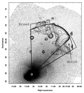
Figure 3.— Shapes of the elliptical annular wedges used to derive the radial X-ray surface brightness profile across the radio relic are shown. The greyscale image is the XMM-Newton X-ray image with the point sources removed. The contours are the SUMMS 843 MHz radio image. The solid lines show the shape of the default elliptical wedges used to derive the surface brightnesses; the wider region includes the “notch” in the radio relic, while the narrower region excludes it. This wider region was also used to accumulate the full cluster profile in the NW regions (§ 3.1). The dashed curve shows the “broad” region for the relic, including the radio extension to the NE. In each case, the elliptical wedge shown corresponds to our adopted shape for the outer edge of the radio relic. The regions all start at the cluster pressure peak, which is indicated by the white circle.

3.2. X-ray Surface Brightness Profile across the Relic

The radial X-ray surface brightness profile across the NW radio relic was determined in the 0.5–2.0 keV band (excluding the Al line at $\sim$1.5 keV). The surface brightness was corrected for exposure and background. We assumed that the X-ray surface brightness is constant on self-similar ellipses. The shape of the ellipses was taken to match approximately the sharp outer edge of the radio relic. The surface brightness was accumulated in elliptical pie annuli (“epanda” regions). In Figure 3, the ellipses shown correspond to our estimates of the outer edge of the relic.

Figure 4.— Radial X-ray surface brightness profile of Abell 3667 from the cluster center to beyond the NW radio relic. The profile has been corrected for exposure and background, and point sources have been removed. The approximate positions of the top of the Mushroom feature and the Shock are indicated. The NW radio relic lies roughly between these two features.

For all these regions, the major axis of the ellipse had a position angle of $-$33^∘ measured from north to east. As a default, we considered a wedge whose width was taken to be approximately the full width of the relic. This wedge extends from an angle of $-$26^∘ to $+$34^∘ of the semi-major axis (measured counter-clockwise).

The values of the surface brightness are shown in Figure 5. The radii $r$ and $r_{\rm relic}$ are measured along the semi-major axis. In the inner part of the profile, the bins had a width of 20″, and they increased in the outer parts to maintain a reasonable signal to noise ratio. Note that the uncertainties increase dramatically for the outer points where the surface brightness is quite low. The surface brightness profile is concave downward and then changes slope at a radius which is close to the outer edge of the relic.

We initially attempted to fit the profile with a standard “beta-model”. This gave a poor fit, with a $\chi^{2}$/dof = 5.16. The value of the core radius was very small and undetermined, since the profile here only included the outer parts of the cluster. The value of $\beta$ was remarkably large, $\beta=2.63\pm 0.06$. This implies a very steep fall-off in the gas density in these regions. With the small value of the core radius, the beta-model reduces to a power-law. The X-ray surface brightness for the beta-model at large radii varies as $I_{X}\propto r^{-6\beta+1}$, which gives a variation of roughly $I_{X}\sim r^{-15}$. Because uncertainties on the surface brightness grow rapidly with radius, the best-fit beta-model is essentially a power-law which fits the inner points of the profile in Figure 5, but lies above all of the data points are large radii. Thus, the beta-model fit misses completely the concave downward drop and change in slope of the observed surface brightness.

Figure 5.— Radial X-ray surface brightness profile across the radio relic in the 0.5–2.0 keV band, excluding the Al line at $\sim$1.5 keV. The profile was corrected for exposure and background, and point sources were removed. The crosses give the data points, with 1-sigma uncertainties and the widths of the bins shown. An emissivity jump is evident very near to the outer edge of the relic ($r_{\rm relic}$), which we interpret as a shock. The solid curve is the best-fit surface brightness model for an ellipsoidal emissivity edge. The vertical line is the estimated position of the outer edge of the radio relic ($r_{\rm relic}=2070\arcsec$), which is just outside of (but consistent within the errors with) the X-ray edge.

To fit this discontinuity, we assumed that the X-ray emissivity is constant on self-similar ellipsoidal surfaces, and that a principal axis of these ellipsoids is in the plane of the sky. The ellipsoidal surfaces are assumed to be symmetric about this principle axis, so that the surfaces of constant emissivity are actually prolate or oblate spheroids, and the extent along the line-of-sight is that same as the projected extent on the sky. The elliptical shapes of the projection of the ellipsoids on the sky was taken to be similar to the outer edge of the relic (the ellipses in Fig. 3). This simple, self-similar ellipsoidal model represents a significant source of systematic errors in our analysis. Some of these assumptions (the extent along the line-of-sight) affect the the overall scale of the emission (e.g., the gas densities may all be off by a constant factor), but some of the other assumptions may affect the shock jump conditions we derive.

We assume that the emissivity had an ellipsoidal discontinuity, but was a power-law function of the elliptical radius inside and outside of this discontinuity. If $r_{\rm edge}$ is the radius of this discontinuity, then the X-ray emissivity was assumed to vary as

$$\epsilon(r)=\left\{\begin{array}[]{ll}\epsilon_{i}(r/r_{\rm edge})^{-2p_{i}}&r<r_{\rm edge}\\ \epsilon_{o}(r/r_{\rm edge})^{-2p_{o}}&r>r_{\rm edge}\,.\end{array}\right.$$ (1)

The X-ray surface brightness is then given by

$$I_{X}(r)=I_{\rm in}(r)+I_{\rm out}(r)\,,$$ (2)

where

$$I_{\rm in}(r)=I_{i}A^{-2p_{i}+1}\left\{\begin{array}[]{ll}1-I_{A^{2}}(p_{i}-\frac{1}{2},\frac{1}{2})&A^{2}<1\\ 0&A^{2}\geq 1\,,\end{array}\right.$$ (3)

and

$$I_{\rm out}(r)=I_{o}A^{-2p_{o}+1}\left\{\begin{array}[]{ll}I_{A^{2}}(p_{o}-\frac{1}{2},\frac{1}{2})&A^{2}<1\\ 1&A^{2}\geq 1\,.\end{array}\right.$$ (4)

Here, $A\equiv(r/r_{\rm edge})$, $I_{x}(a,b)\equiv B_{x}(a,b)/B(a,b)$ is the normalized incomplete beta function, $B_{x}(a,b)\equiv\int_{0}^{x}t^{a-1}(1-t)^{b-1}\,dt$ is the incomplete beta function, $B(a,b)=\Gamma(a)\Gamma(b)/\Gamma(a+b)$ is the beta function, and $\Gamma(a)$ is the gamma function. For details and the expressions for accumulating counts in bins, see Appendix A and also Vikhlinin et al. (2001a) and Korngut et al. (2011). The value $I_{o}$ gives the surface brightness at the edge, while

$$I_{i}=R\,I_{o}\frac{B(p_{i}-\frac{1}{2},\frac{1}{2})}{B(p_{o}-\frac{1}{2},\frac{1}{2})}$$ (5)

normalizes the surface brightness due to gas within the edge. Here, $R\equiv\epsilon_{i}/\epsilon_{o}$ gives the jump in X-ray emissivity at the edge.

Table 1Radio Relic and Mushroom X-ray Surface Brightness Profile Fits

	$r_{\rm edge}$	$\Delta r_{\rm edge}$				$I_{o}$
Region	(arcsec)	(arcsec)	$p_{i}$	$p_{o}$	Ratio $R$	($10^{-8}$ cts s-1 arcsec-2)	$\chi^{2}$/dof
Relic with notch	$2053^{+17}_{-20}$	$-17^{+17}_{-20}$	$+3.40^{+0.09}_{-0.10}$	$3.30^{+1.10}_{-1.02}$	$3.11^{+1.75}_{-0.94}$	0$2.61^{+0.67}_{-0.53}$	051.94/32 $=$ 1.654
	(2070)	(0)	$+3.43^{+0.09}_{-0.09}$	$2.88^{+1.06}_{-0.94}$	$3.74^{+2.20}_{-1.13}$	0$2.22^{+0.41}_{-0.39}$	054.60/33 $=$ 1.894
	(2070)	(0)	$+3.57^{+0.25}_{-0.25}$	$8.68^{+5.13}_{-2.41}$	(1)	0$4.04^{+0.53}_{-0.66}$	102.60/34 $=$ 3.018
Relic without notch	$2059^{+28}_{-23}$	$-11^{+28}_{-23}$	$+3.39^{+0.13}_{-0.14}$	$3.56^{+2.43}_{-2.55}$	$4.73^{+18.71}_{-2.52}$	0$1.02^{+0.62}_{-0.45}$	059.89/32 $=$ 1.871
	(2070)	(0)	$+3.41^{+0.11}_{-0.12}$	$2.86^{+2.86}_{-2.31}$	$6.43^{+96.77}_{-2.96}$	0$0.84^{+0.39}_{-0.34}$	060.73/33 $=$ 1.840
Relic, broad region	$2034^{+30}_{-27}$	$-36^{+30}_{-27}$	$+3.69^{+0.13}_{-0.12}$	$3.29^{+1.57}_{-1.73}$	$2.90^{+3.81}_{-1.04}$	0$2.22^{+0.76}_{-0.67}$	076.85/32 $=$ 2.402
	(2070)	(0)	$+3.76^{+0.10}_{-0.11}$	0$2.43^{+1.78}_{-1.69}$	$4.24^{+17.18}_{-1.86}$	0$1.66^{+0.47}_{-0.44}$	080.92/33 $=$ 2.452
Mushroom	$1503^{+4}_{-5}$		$-0.13^{+0.08}_{-0.09}$	0$3.06^{+0.22}_{-0.20}$	$2.75^{+0.25}_{-0.25}$	$44.3^{+2.2}_{-1.8}$	055.38/36 $=$ 1.538
	(1503)		$+0.53^{+0.06}_{-0.06}$	0$5.43^{+0.12}_{-0.12}$	(1)	$65.8^{+0.7}_{-0.7}$	698.66/38 $=$ 18.396

This surface brightness model was convolved with the PSF of XMM-Newton (Read et al. 2011), and then accumulated in the bins used to determine the observed surface brightness (see Appendix A for details). The variable parameters of the model were taken to be the radius of the edge ($r_{\rm edge}$), the emissivity power-law exponents within and outside of the edge ($p_{i}$ and $p_{o}$, respectively), the emissivity jump at the edge $R$, and the surface brightness at the edge ($I_{o}$). Because the value of $r_{\rm edge}$ is measured from the somewhat arbitrary center of the ellipse used to fit the outer edge of the radio relic, we instead report the value of $\Delta r_{\rm edge}\equiv r_{\rm edge}-r_{\rm relic}$, where $r_{\rm relic}$ is the radius of the outer edge of the radio relic as shown in Figure 3. The model parameters were varied until the value of $\chi^{2}$ was minimized. The uncertainty (90% confidence) in each of the parameters was determined by varying all of the variables, and determining the width of the surface where the value of $\chi^{2}$ was increased by 2.706, marginalizing over all the other parameters. The best-fit values of the parameters, the minimum value of $\chi^{2}$, and the number of degrees of freedom (dof) are all given in Table 1.

We first considered regions which were essentially the full width of the radio relic, and which fit well the sharp outer edge at the center of the relic (the wider solid lines in Fig. 3). The fits to this surface brightness profile (shown in Fig. 5) are listed in the first two lines of Table 1 and labelled “Relic with notch”. We first allowed all of the parameters to vary. This fit is shown in the first line of Table 1, and in Figure 5. The value of $\chi^{2}$ is somewhat high, and the deviations are due to both some inner points where it is likely that other X-ray structures occur and the statistical errors are small, and to the outermost points where the statistics are not very good. The emissivity exponents $p_{i}$ and $p_{o}$ correspond to the variation of the gas density with radius at a fixed temperature and abundances. The two values are consistent within the errors. When compared to a beta-model at large radii, the emissivity exponents are $p=3\beta$. Thus, the fitted exponents are consistent with $\beta\approx 1.1$, which is fairly large. This indicates that the gas density is dropping rapidly with radius at this location, which is near the virial radius of the cluster.

The fitted value of the radius of the edge is very close to the outer radius of the radio relic, and the two appear to be consistent within the uncertainties. To test this, we set $r_{\rm edge}=r_{\rm relic}$, fixed this parameter, and redid the fit. This fit is shown in the second line of Table 1. All of the parameters of this fit are consistent with those of the previous fit with a variable $r_{\rm edge}$ within the uncertainties. Although the value of $\chi^{2}$/dof for this fit is slightly worse than that for the variable $r_{\rm edge}$, the f-test indicates that the probability that the fit with a fixed $r_{\rm edge}$ is at least as good as the fit with a variable $r_{\rm edge}$ is 21%, which is not terribly low. Thus, the X-ray surface brightness edge is located at the outer edge of the radio relic to within the errors.

The best-fit values of $R$ are larger than unity by about 4-sigma. As another test for the reality of the edge, we redid the fit, fixing the value of $r_{\rm edge}=r_{\rm relic}$, and fixing $R=1$. As shown in line 3 of Table 1, this is a very poor fit to the observed surface brightness profile. The f-test indicates that the probability that there is no X-ray edge at the outer radius of the radio relic is only $2\times 10^{-5}$.

As noted above, the NW radio relic has a “notch” at its southwest end which breaks the relatively smooth curve of the outer edge of the relic. It is unclear whether this feature is due to a disturbance in the hydrodynamics of the ICM, or due to the geometry of pre-existing relativistic particles and magnetic field, or a projection effect (e.g., the notch is due to emission on the front or back side of a curved shock feature. In an effort to eliminate these sources of systematic uncertainty, we also determined the radial X-ray surface brightness profile in a narrower elliptical wedge which excluded the notch (narrower solid lines in Fig. 3). This wedge extended from an angle of $-$13.5^∘ to $+$34^∘ of the semi-major axis (measured counter-clockwise). The results of a fit to the surface brightness profile in this wedge are shown in line 4 of Table 1. This fit is significantly worse than the fit including the notch, and the uncertainties in the parameters are increased, in some cases very significantly. Except for the surface brightness, the edge parameters are consistent with the values of the whole wedge. However, the X-ray surface brightness in the outer regions is lower, and the errors are thus much larger. In particular, the uncertainties in the value of the $R$ are quite large; this is the most important quantity in this fit, since it determines the compression and Mach number of the shock (see §§ 5.1 & B.1 below). However, the possibility that there is no edge (R $=$ 0) can be ruled out with high confidence (probability $<1$% by the f-test).

We also extracted the surface brightness profile for the notch region alone (angles between $-$26^∘ and $-$13.5^∘ of the semi-major axis; Fig. 3). This surface brightness profile showed the same shock feature at essentially the same radius (the best fit radius was smaller by about 4%). However, because the area covered was about a factor of five smaller, the statistics were worse. There also was a feature at the top of the Mushroom which is discussed in more detail below (§ 3.3). The outer edge of the Mushroom corresponds approximately to the inner edge of the notch in the radio relic. There was no clear feature at the outer edge of the radio relic, as might have been expected if this edge also marked the position of a shock.

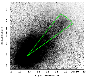
Figure 6.— Shape of the elliptical annular wedges used to derive the radial X-ray surface brightness profile across the Mushroom feature. The greyscale image is the XMM-Newton X-ray image with the point sources removed. The solid green lines show the shape of the elliptical wedges used to derive the surface brightnesses. The radius of this elliptical wedge corresponds to the best-fit outer radius (semi-major axis of the ellipse) of 1503″. The elliptical wedge starts at the cluster pressure peak (see Fig. 3).

We also consider a set of broader elliptical pie annuli which include the extension of the radio relic to the NE (dashed lines in Fig. 3). This was a considerably worse fit (line 6 in Table 1). Moreover, the best-fit location of the edge was $\sim$36″ inside of the outer edge of the radio relic. This suggests that broadening the adapted outer limit of the radio relic to include the NE extension to the radio relic moved this radius beyond the actual X-ray edge at the two ends of the relic. Also, the value of $R$ was poorly determined. If the location of the edge was fixed to the the adopted outer radius of the radio relic, the fit was only slightly worse, but the value of $R$ was nearly unconstrained (line 7 of Table 1). The possibility that there was no edge could again be ruled out with high confidence (probability $<0.3$%), but the strength of the jump could be very large. As noted above, $R$ is the most important parameter for the physical interpretation of the emission edge. These results suggest that the broader region did not fit the shape of the X-ray edge as well as our standard “Relic with notch” region. Thus, we will use the values in line 1 of Table 1 as the standard parameters of the surface brightness edge.

Note that one key assumption in this analysis is that the principle axis of the emissivity edge is in the plane of the sky. For other orientations, projection effects weaken the surface brightness discontinuity. Thus, it is likely that the fitted values of $R$ underestimate the actual emissivity jump.

Figure 7.— Radial X-ray surface brightness profile across the Mushroom feature in the 0.5–2.0 keV band, excluding the Al line at $\sim$1.5 keV. The profile was corrected for exposure and background, and point sources were removed. The notation is the same as in Fig. 5. The vertical line is the best-fit radius of the top of the Mushroom. An emissivity jump is evident at the top of the Mushroom.

3.3. X-ray Surface Brightness Profile across the Mushroom

The radial surface brightness profile along the Mushroom feature was also extracted. The shape of the elliptical wedge annular (epanda) regions used to accumulate the surface brightness in the region of the Mushroom is shown in Figure 6. The technique and model assumptions are the same as for the radial profile of the radio relic region (§ 3.2), The resulting surface brightness profile is given in Figure 7.

The surface brightness profile shows the characteristic shape associated with a curved surface discontinuity in the X-ray emissivity. The same model for an emissivity profile which has a discontinuity and is a power-law function of radius was fit to this data. The best-fit model is shown in Figure 7 and the parameters are given in row 8 of Table 1. The best-fit emissivity jump is a factor of $2.75^{+0.25}_{-0.25}$. This is a reasonably good fit. There is clearly some more complicated structure in the surface brightness profile, as is also shown in the image. Note that the profile implies an inner X-ray emissivity which actually rises slightly with increasing radius. This may indicate that the region below the Mushroom is a tail of decreasing density, and that the tail dominates the overall cluster radial surface brightness profile in this region.

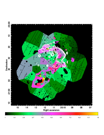
Figure 8.— XMM-Newton temperature map of Abell 3667. The contours are from the SUMSS 843 MHz radio image the NW radio relic. The temperature map shows that the region of the radio relic is hot ($\sim 5$ keV), while the region outside of the relic to the NW is much cooler ($\sim$2 keV). The temperature map also indicates that the Mushroom feature just to the south of the relic is also hot ($\sim$6 keV).

4. X-ray Spectra

The spectra were fit in the energy range 0.8–12 keV, excluding the ranges from 1.35–1.75 keV and 7.5–9.9 keV which contain strong instrumental lines. The foreground/background components included in the fit included the low energy Galactic foreground, particle background, and residual cosmic X-ray background from unresolved AGNs. The upper end of the spectral band was included to provide better constraints on the residual particle and cosmic X-ray backgrounds. The spectra were grouped to have at least 30 raw counts per bin to allow $\chi^{2}$ statistics to be applied. Unless otherwise noted, we assume that the Galactic absorbing column was given by $N_{H}=4.5\times 10^{20}$ cm^-2, and that the abundance of the cluster gas was 0.3 solar.

4.1. Cluster Temperature Map

The resulting temperature map is shown in Figure 8. All detected emission from sources with angular sizes of $\leq$32″ has been excluded from the fit; these sources as well as the gaps in the pn coverage can be seen in Figure 8 as black zones. In general, the outer parts of the cluster are relatively cool, although the errors are large in most directions due to the relatively short exposures in the outer regions except for the NW radio relic region (Fig. 1). The region of the NW radio relic is relatively hot ($\sim 5$ keV), while the region just outside the relic to the NW is quite cool ($\sim$2 keV). This is consistent with the presence of a shock at the outer edge of the radio relic. Note also that the Mushroom region is fairly hot ($\sim$6 keV), which may indicate that this feature is also due to a shock, rather than a cold front.

Figure 9.— Filled circles give the best-fitted XMM-Newton temperatures in elliptical pie annuli regions which cross the NW radio relic as a function of the semi-major axis of the ellipse. The solid vertical line gives the approximate location of the outer edge of the NW radio relic. The widths of the error bars give the regions used to accumulate the spectra, while the vertical error bars are 1–$\sigma$ uncertainties. Note the rise in the temperature within the outer edge of the relic. The error bars without circles are de-projected temperatures for the outer 12 region fit using the projct model in xspec. The horizontal dashed lines show the radial regions used to accumulate the Post-Shock/Relic and Pre-Shock spectra discussed in §§ 4.3 and 4.4. The thin curve shows the non-equipartition model for the post-shock temperature variation (§§ 5.2 & Appendix C), which should be compared to the de-projected data points.

4.2. Temperature Profile Across the Relic

We determined the radial temperature profile across the region of the NW radio relic using elliptical pie annuli with the same shape as those used to accumulate the surface brightness profile in § 3.2. Specifically, we used the standard panda regions in Figure  3 which included the ‘Notch’ region. The elliptical pie annuli were wider radially than those used to determine the SB profile in order to provide enough counts for spectral fitting. Starting at the ellipse which fit the outer edge of the radio relic, we chose epanda regions having a total number of at least 5000 source counts in the 0.5–2.0 keV band. The large number was needed because of the relatively high ratio of background to source counts in these outer cluster regions.

Figure 9 shows the radial temperature profile (filled circle points) across the NW radio relic. The temperature rises from $\sim$1.2 keV to $\sim$4.5 keV just inside of the outer edge of the relic. This indicates that the X-ray emissivity jump seen at the same location (Fig. 5) is a shock. Note, however, that the temperature doesn’t rise discontinuously immediately at the outer edge of the relic, but instead increases over a radial region of about 3 arcmin in width. The best-fitted temperature is then approximately constant for $1450\arcsec\lesssim r\lesssim 1870\arcsec$. At smaller radii, the temperature rises slightly again; Figure 8 indicates that this is mainly due to slightly hotter gas associated with the Mushroom feature.

In principle, the finite point-spread-function (PSF) of XMM-Newton will cause a sharp spectral change to appear more gradual. However, the full-width-half-maximum for the XMM mirrors and detectors is only around 6″, and the half-energy-width is only about 16″. Thus, the PSF only makes a small contribution to the broadening to the temperature rise inside of the shock front.

Table 2Pre-Shock and Post-Shock/Relic X-ray Spectral Fits

	$r_{\rm in}$	$r_{\rm out}$		$kT$	NormT	$kT_{2}$ or $\Gamma$
Region	(arcsec)	(arcsec)	Model	(keV)	($10^{-3}$)	(keV or none)	Norm2	$\chi^{2}$/dof
Pre-Shock	2070	2410	1T	$1.23^{+0.06}_{-0.17}$	$0.214^{+0.007}_{-0.043}$			2551.4/1674 $=$ 1.524
Post-Shock	1450	1870	1T	$4.37^{+0.93}_{-0.76}$	$1.403^{+0.039}_{-0.038}$			2237.9/1639 $=$ 1.365
			2T	$5.35^{+2.23}_{-1.26}$	$1.263^{+0.026}_{-0.026}$	(1.23)	$0.109^{+0.029}_{-0.025}$	2200.1/1638 $=$ 1.343
			2T	$5.68^{+1.69}_{-1.13}$	$1.226^{+0.052}_{-0.036}$	(1.23)	(0.1335)	2202.6/1639 $=$ 1.344
			2T	$5.58^{+2.40}_{-1.39}$	$1.244^{+0.024}_{-0.021}$	$0.95^{+0.02}_{-0.02}$	$0.258^{+0.036}_{-0.045}$	4730.7/3312 $=$ 1.428
			1TPL	$6.11^{+3.51}_{-1.65}$	$1.213^{+0.035}_{-0.064}$	$5.21^{+0.45}_{-0.74}$	$1.35^{+0.43}_{-0.19}$	2195.5/1637 $=$ 1.341
			1TPL	$8.33^{+7.43}_{-4.50}$	$0.497^{+0.188}_{-0.079}$	(2.10)	$2.45^{+0.38}_{-0.59}$	2210.1/1638 $=$ 1.349

The accumulated spectra include emission along the entire line-of-sight, and thus contain emission from gas at larger radii. We have determined the best-fitted temperatures by de-projecting these spectra. In doing this, we made the same assumptions used to de-project the X-ray SB profile to give the emissivity in § 3.2: that the temperature is constant on aligned self-similar prolate spheroidal surfaces whose shape is given by the outer edge of the NW radio relic, and that the major axis of the prolate spheroid is in the plane of the sky. The error bars without filled circles show the best-fitted de-projected temperatures determined using the projct function in xspec. We also did the de-projection using the “onion-peeling” algorithm discussed in Blanton et al. (2003), which is more robust and stable when there are large gradients in the X-ray SB. Both techniques gave very similar results. While projection can account for a non-trivial portion of the broadening, the temperature still increases over a radius of about 2′. The effect of projection will increase if the major axis of the shock front is not in the plane of the sky, and this might account for the broadening. More generally, other breakdowns in the simple ellipsoidal X-ray emissivity model we have assumed might have the effect of broadening the observed temperature profile. However, this would also affect the SB profile, which is reasonably well-fitted by the simple projection model (Table 1 and Fig. 5). The absence of large gradients in the radial velocity distribution of the galaxies also suggests that the merger is nearly in the plane of the sky (Johnston-Hollitt 2004).

The broadening of the temperature profile at the outer edge of the relic may also be due to inhomogeneities in the temperature structure of the gas, either on the plane of the sky (e.g., the ‘Notch’ feature in the relic) or along the line-of-sight. Possible physical explanations for the temperature profile are discussed in § 5.2.

4.3. Pre-Shock X-ray Spectrum

We also determined the X-ray spectrum of the gas just beyond and just within the outer edge of the NW radio relic. For this purpose, we used larger regions to provide a more accurate determination of the temperature and other properties. The resulting fits are summarized in Table 2.

For the gas just beyond the relic (the “Pre-Shock” gas), we fit the spectrum in an elliptical pie annulus extending from 2070″ to 2410″  (Fig. 9). While this gave a fit that agreed well with the values in Figure 9, the $\chi^{2}$ value was rather high, suggesting that there are remaining systematic uncertainties in the background. The regions used to accumulate the pre- and post-shock spectra are large enough that the statistical errors in the spectra are fairly low. But, given the low cluster surface brightness at these large radii, systematic errors in the background are likely to be important. Therefore, we included a systematic error of 3% in the background correction when determining the errors in the fit parameters. The values of $\chi^{2}$ include only the statistical errors. This gave a pre-shock temperature of $kT=1.23^{+0.06}_{-0.17}$ keV. If the abundance was allowed to vary, the best fit value was $0.075\pm 0.013$, but the fit was not improved significantly. This is a rather low abundance, but perhaps not unreasonable for gas $\sim$2.3 Mpc from the cluster center.

4.4. Post-Shock/Relic X-ray Spectrum

The spectrum of the post-shock gas was extracted from an elliptical pie annulus extending from 1450″ to 1870″  (Fig. 9). The outer edge of this region is well within the apparent shock location from the X-ray surface brightness profile or the outer edge of the radio relic. The reason for this choice is the rather extended rise in the temperature as seen in the temperature profile. This rise might be due in part to the finite spatial resolution of XMM-Newton, although the angular region of the rise is too broad for this to be the main cause. It is partially due to projection effects, although Figure 9 suggests that this is not the sole cause. It may be due to temperature inhomogeneities due to structure in the shock front, such as the Notch. It may have another astrophysical cause (§ 5.2), such as electron-ion non-equipartition at the shock. In any case, it seemed safer to exclude the transition region, and extract the post-shock spectrum from the region after the temperature profile has flattened. This post-shock region still includes 59% of the radio flux of the relic.

4.4.1 Post-Shock Thermal Emission

The post-shock spectrum was fit initially with a single temperature model. The best-fit model had a temperature of $kT=4.37^{+0.93}_{-0.76}$ keV (row 2 in Table 2), which is consistent with the results from the temperature profile (Fig. 9). This fit is shown in Figure 10. If the abundance is allowed to vary, the best fit value is $0.08\pm 0.03$ solar, which is low but consistent with the pre-shock spectral fits. If the abundance is fixed at 0.3 solar, the temperature is $kT=4.80^{+0.20}_{-0.13}$ keV, and the fit is only slightly worse.

We next tried a two-temperature fit to the spectrum. However, the temperatures were not well constrained. One motivation for a two temperature model is that some of the pre-shock gas is almost certainly projected onto the post-shock region. Thus, we also tried a two temperature fit in which the outer thermal component was fixed to the spectrum of the pre-shock gas (row 1 in Table 2). Initially, the normalization of this second, cooler component was allowed to vary. This resulted in a higher temperature ($kT=5.35^{+2.23}_{-1.26}$ keV; row 3 in Table 2) as expected. The flux of the best-fit cool component was reasonably close to what one might expect from projection, if one assumes that the geometry and gas density distribution were given by the best-fit X-ray surface brightness model near the shock (§ 3.2 and Table 1), and one assumes that all of the pre-shock gas has the same spectrum. The surface brightness model predicts that the normalization of the cool gas projected on the post-shock spectral regions is 0.62 times the normalization in the pre-shock spectral region. This gives a normalization of 0.1335 (in the units in Table 2), whereas the best-fit value is 0.109.

We also fixed the spectrum and normalization of the cool component in the post-shock regions to the spectrum of the pre-shock gas and the normalization predicted by the X-ray surface brightness model (row 4 in Table 2). This was only a slightly worse fit with a consistent temperature $kT=5.68^{+1.69}_{-1.13}$ keV. This result corresponds to the “onion-peeling” spectral de-projection algorithm discussed in Blanton et al. (2003).

Finally, we fit the pre- and post-shock spectra simultaneously, including the pre-shock gas in the projected post-shock spectra based on the model for the X-ray surface brightness (row 5 in Table 2). This gave a consistent value for the de-projected post-shock temperature ($kT=5.58^{+2.40}_{-1.39}$ keV), but a considerably lower temperature for the pre-shock gas. Because we believe it is safer to determine the temperature of the pre-shock gas purely from a region containing only that gas, we prefer the previous fit (row 1 in Table 2). However, the xspec fit gave a value for the covariance between the pre- and de-projected post-shock temperatures of $\sigma(T_{1},T_{2})=-6.00\times 10^{-6}$ keV², which is useful for the subsequent analysis.

4.4.2 Post-Shock IC Emission

The same relativistic electrons which produce the synchrotron radio emission of the radio relic will also produce X-ray emission by inverse Compton (IC) scattering of Cosmic Microwave Background photons. For reasonable values of the magnetic field, X-ray emission in the XMM-Newton band will be produced by lower energy relativistic electrons than those which generate the radio emission in the observed images. Thus, the post-shock region may also have some IC emission, as well as the thermal emission from the shocked intracluster gas. To search for this emission in the post-shock spectrum, we have included a power-law spectral component in our models. Initially, we allowed both the photon spectral index $\Gamma$ and the normalization of the power-law component to vary during the fit. This results in a power-law spectrum with an unphysical steep spectral index, $\Gamma=5.21^{+0.45}_{-0.74}$ (row 7 in Table 2). This power-law component only affects the softest X-ray channels in the spectrum. The fitted spectral index is much higher than that of the radio relic synchrotron spectrum. For synchrotron and IC emission from the same relativistic electrons, the radio and X-ray spectral indices should agree. Since the IC X-ray emission here should actually come from somewhat lower energy electrons than the radio emission, one might expect the IC spectral index to actually be a bit smaller than the radio value. Thus, we fixed the IC spectral index the observed radio value of $\Gamma=2.1$ (Röttgering et al. 1997). This led to a fit (row 8 in Table 2) in which roughly half of the flux comes from the non thermal component. However, the temperature of the thermal ICM is then very high ($\sim$8 keV, but with very large uncertainties), which might be inconsistent with the intracluster gas temperatures at slightly smaller radii or with the jump conditions for a shock with a Mach number consistent with the gas density jump. The 1TPL fit is better than the 1T fit, but only slightly.

Another issue with a large IC contribution to the post-shock spectrum is the slow rise in temperature behind the shock (Fig. 9 and §§ 4.2 & 5.2). For a power-law energy distribution of relativistic electrons, the radio synchrotron and X-ray IC emission have the same power-law spectral shape. The radio spectrum immediately behind the shock is fairly flat (Johnston-Hollitt 2004), which suggests the IC spectrum should also be quite hard. The relic radio spectrum steepens with distance from the shock, and this is consistent with energy losses by the relativistic electrons behind the shock (§ 5.4). Thus, if anything, the X-ray IC spectrum should become softer further behind the shock. But, the observed spectra actually gets harder (Fig. 9). This suggests that the majority of the post-shock X-ray emission is not due to IC.

Given these issues, we treat the flux of the possible IC component at an upper limit. This gives an upper limit on the IC photon flux of $<3.2\times 10^{-4}$ cts cm^-2 s^-1 or an energy flux of $<1.0\times 10^{-12}$ erg cm^-2 s^-1 (0.8–8.0 keV, unabsorbed, 90% confidence level). Since the post-shock spectral region includes only 59% of the radio relic flux, the limit of the total IC flux would be $<5.4\times 10^{-4}$ cts cm^-2 s^-1 ($<1.7\times 10^{-12}$ erg cm^-2 s^-1) assuming the IC X-ray flux is proportional to the radio flux. This limit is similar to previous limits (Nakazawa et al. 2009, FSN), and implies a lower limit on the magnetic field in the relic of $B\gtrsim 3$ $\mu$G. The upper limits from the lack of Faraday rotation are similar (Johnston-Hollitt 2004), which suggests that $B\sim 3$ $\mu$G. We will assume this value in further discussions.

Figure 10.— Best-fit single temperature model for the post-shock spectrum (row 2 in Table 2). The upper panel gives the data and the model. The lower solid curve is the model for the cluster emission, while the upper curve gives the total model including background. The lower panel gives the residuals to the fit, in terms of the contribution to $\chi^{2}$, multiplied by the sign of the residual.

4.5. Mushroom Spectra

The radial temperature profile of the gas in the Mushroom was determined from spectra accumulated in epanda regions with the same shape as those used to determine the radial X-ray surface brightness profile (§ 3.3). Wider annuli were used for the spectra since more counts are needed to derive temperatures. The techniques were the same as those used to derive the radial temperature profile across the radio relic region (§ 4.2). The resulting temperature profile is shown in Figure 11. While there is a suggestion that the gas just above the Mushroom is hotter than the gas within it, the trend is not very clear.

Figure 11.— The radial temperature profile across the Mushroom feature. The solid vertical line gives the best-fit radius of the top of the Mushroom as determined from the radial surface brightness profile. The widths of the error bars give the regions used to accumulate the spectra, while the vertical error bars are 1–$\sigma$ uncertainties. No very clear temperature trend is obvious.

5. Discussion

5.1. Shock Jump Conditions

Both the surface brightness profile (Fig. 5) and the temperature profile (Fig. 9) show a discontinuity at the location of the outer edge of the radio relic, which indicates that a shock is present there. The jump in the X-ray emissivity and the jump in temperature each provide a nearly independent estimate of the shock Mach number ${\cal{M}}$.

The jump in the X-ray emissivity at the shock found from the X-ray surface brightness profile is $R=3.11^{+1.75}_{-0.94}$ (§ 3.2, Table 1). This ratio must be corrected for the temperature-dependent emission function of the gas (Eq. B1). Following the procedure in Appendix B.1, we find $(\Lambda_{2}/\Lambda_{1})=0.57^{+0.04}_{-0.10}$. This gives a shock compression $C\equiv\rho_{2}/\rho_{1}=2.34^{+0.69}_{-0.36}$, where $\rho$ is the gas mass density, and the subscripts 1 and 2 refer to the pre- and post-shock gas, respectively. The shock Mach number is then ${\cal{M}}=2.05^{+0.73}_{-0.38}$.

The pre- and post-shock temperatures are $kT_{1}=1.23^{+0.06}_{-0.17}$ keV (row 1 in Table 2) and $kT_{2}=5.35^{+2.23}_{-1.26}$ keV (row 3 in Table 2), respectively. For the post-shock temperature, we use the value de-projected by fitting the projected spectrum to the pre-shock spectral shape (with a variable normalization) plus the post-shock spectrum. As noted in § 4.4.1, the normalization of the pre-shock spectrum in this fit is within 20% of the value predicted by the best-fit X-ray surface brightness profile (§ 3.2). But, fitting the normalization from the observed post-shock spectra should help to insure against small differences in the pre-shock gas distribution along the line-of-sight to the post-shock spectral region. The effects of projection are somewhat reduced by the fact that our chosen post-shock spectral region is displaced inwards from the shock front, and the X-ray surface brightness profile declines rapidly. This gives a temperature ratio of $(T_{2}/T_{1})=4.35^{+1.91}_{-1.05}$. The shock jump conditions then imply a Mach number of ${\cal{M}}=3.34^{+0.91}_{-0.50}$. The Mach number from the temperature jump is 1.46 $\sigma$ higher than the value from the X-ray surface brightness jump. The mean shock number from these two values weighted by their errors is ${\cal{M}}=2.54^{+0.80}_{-0.43}$, which we adopt as our best value for further analysis. Although the uncertainties are large, this Mach number makes the NW Relic shock in Abell 3667 one of the strongest shocks seen in a cluster, although weaker than that in the Bullet Cluster (${\cal{M}}=3.0\pm 0.4$; Markevitch & Vikhlinin 2007).

This Mach number implies a shock compression of $C=2.73^{+0.55}_{-0.29}$, and a temperature jump of $(T_{2}/T_{1})=2.86^{+1.29}_{-0.69}$. The pre-shock sound speed is $c_{s}=569^{+14}_{-39}$ km s^-1, which implies a shock speed of $v_{s}={\cal{M}}c_{s}=1450^{+460}_{-260}$ km s^-1. The speed of the post-shock gas relative to the shock is then $v_{2}=v_{s}/C=530^{+60}_{-50}$ km s^-1.

Our fit to the X-ray surface brightness also allows the pre- and post-shock densities to be determined. Our best-fit model gave a surface brightness at the shock apex of $I_{o}=(2.61^{+0.67}_{-0.53})\times 10^{-8}$ cts s^-1 arcsec^-2 (Tab. 1). This implies a pre-shock electron density of $n_{e1}=5.51\times 10^{-5}$ cm^-3 from equations (A3) and (A12) in Korngut et al. (2011). The post-shock electron density is $n_{e2}=Cn_{e1}=1.51\times 10^{-4}$ cm^-3.

The measured values of the density and temperature jump at the shock are somewhat inconsistent for a $\gamma=5/3$ shock. The temperature jump is larger than expected given the density jump, which could mean that the gas is “less isothermal”, which suggests that the effective adiabatic index is $\gamma_{\rm eff}>5/3$. If one assumes that the shock compression and temperature jump are consistent (§ B.4), the implied effective adiabatic index and shock Mach number are $\gamma_{\rm eff}=2.05^{+0.32}_{-0.52}$ and ${\cal{M}}=2.80^{+0.76}_{-0.50}$. If the shocked gas contained a significant energy density of relativistic particles or turbulent magnetic fields, one might expect a value of $\gamma_{\rm eff}\approx 4/3$, which is the opposite trend from what is observed. However, if there is a strong, ordered magnetic field, particularly parallel to the shock front, then one would expect $\gamma_{\rm eff}\approx 2$, which is close to the required value (Helfer 1953). Thus, the shock jump conditions might provide some evidence for a dynamically important, ordered magnetic field with a significant component parallel to the shock front. This would also be consistent with the the observed radio polarization of the radio relic just behind the shock front (Johnston-Hollitt 2004).

The measured X-ray surface brightness and temperature jump were fit simultaneously to a shock model with a magnetic field which is parallel to the shock front (§ B.5). This model had a ratio of magnetic to gas pressure of $b\approx 3.55$, and a shock Mach number of ${\cal{M}}\approx 5.12$, giving a shock velocity of $v_{s}\approx 2920$ km s^-1. Although not ruled out by present observations, the magnetic field strength and shock speed are both rather large. Thus, with the fact that the temperature jump is larger than expected for the density jump in Abell 3667 would be consistent with a dynamically non-trivial magnetic field aligned roughly parallel to the shock front, the large errors make any conclusion uncertain. Additional deep observations of other merger shocks would be useful to see if there is a consistent pattern of large temperature jumps relative to the X-ray surface brightness jumps.

Since the difference in Mach numbers from the density and temperature jump are only mildly inconsistent, and the parameters of the ordered magnetic field model seem too extreme, we will continue to use the average shock properties from the temperature and density jump in the subsequent analysis.

5.2. Temperature Profile at Shock

As noted in § 4.2 and Figure 9, the temperature increase within the shock is more gradual than might have been expected given the XMM-Newton PSF. Much of the slow rise in temperature can be explained by the projection of pre-shock gas in front of and behind the shock (the lighter error bars without circles in Fig. 9). However, the de-projected temperature profile still requires about 2$\farcm$3 to rise from the pre-shock value to a plateau at the post-shock value.

One simple explanation for the slow rise in the temperature would be inhomogeneities in the gas near the shock surface, either along our line-of-sight or in the plane of the sky. One obvious inhomogeneity is the Notch at the western end of the radio relic (e.g., Fig.  3). This feature extends roughly 5′ within the assumed elliptical shock surface. The temperature map (Fig.  8) does suggest that the gas in this region is cooler than the remainder of the shock.

Alternatively, it is uncertain how effective collisionless astrophysical shocks are at heating electrons. If the electrons are not heated very effectively in the shock, then given the very low gas densities in this region roughly 2.2 Mpc from the center of the cluster and the high shock speed, it is possible that the post-shock gas has not had time to come into electron-ion equipartition by Coulomb collisions, or into collisional ionization equilibrium. If the electrons are not strongly heated by the shock, the time scale for the electron and ion temperatures to come into equipartition is approximately (Fox & Loeb 1997; Wong & Sarazin 2009)

$$t_{\rm eq}\approx 6.3\times 10^{7}\left(\frac{T_{e}}{10^{7}\,{\rm K}}\right)^{3/2}\left(\frac{n_{p}}{10^{-4}\,{\rm cm}^{-3}}\right)^{-1}\left(\frac{\ln\Lambda}{40}\right)^{-1}\,{\rm yr}\,,$$ (6)

where $T_{e}$ is the electron temperature, $n_{p}$ is the proton density, and $\ln\Lambda$ is the Coulomb logarithm. Because the merger shock has a relatively low Mach number (as is true of all merger shocks), the electrons will be heated significantly by adiabatic compression, even if there were no shock electron heating. For the adapted value for the shock compression, adiabatic heating gives $(T_{e2}/T_{e1})\approx 1.95^{+0.26}_{-0.14}$, while the full shock heating including adiabatic compression gives $(T_{2}/T_{1})=2.86^{+1.29}_{-0.69}$. If the adapted post-shock density and the post-shock electron temperature assuming only adiabatic heating are used in equation (6), the approximate time to reach equipartition is $t_{\rm eq}\approx 2.4\times 10^{8}$ yr. Thus, the thickness of the region with a lowered electron temperature would be $d_{\rm eq}\approx v_{2}t_{\rm eq}\approx 0.13$ Mpc, corresponding to an angular scale of $\theta_{\rm eq}\approx 2.1\cos\phi$ arcmin, where $\phi$ is the angle between the central shock normal and the plane of the sky. Combined with the effects of projection (Fig. 9), non-equipartition could explain the width of the region over which the observed X-ray spectral temperature rises within the shock.

In Figure 9, the narrow curve gives the expected variation in the electron temperature behind the shock due to non-equipartition. The assumptions are that the total electron plus ion temperature (the total thermal energy) behind the shock is constant and given by the de-projected temperature from the post-shock spectrum (row 3 of Table 2), that the gas density increases as an inverse power-law of radius (Tab. 1), and that our best-fit values of $n_{e2}$, $T_{2}$, $T_{1}$, shock compression $C$, and shock speed $v_{s}$ are all correct, and that the apex of the shock lies in the plane of the sky. Given that there are no free parameters in this Coulomb heating model, it may not be surprising that this is not a very good fit. However, its biggest flaws are the jump in electron temperature at the shock due to adiabatic compression, and the subsequent rapid increase in the temperature within the shock. The overall rapid increase in the temperature in the model compared to the de-projected spectral fits suggest that non-equipartition is not the primary cause of the slow temperature rise.

Another result of the low gas density and high shock speed in the relic shock is a departure from collisional ionization equilibrium. Unlike non-equipartition (which will not be important if electrons are effectively heated in the shock) or transport processes such as thermal conduction (which can be greatly reduced in importance by magnetic effects), non-equilibrium collisional ionization is certain to occur in low density shocks. However, if the pre-shock gas temperature is high, most of the X-ray emission is due to thermal bremsstrahlung rather than line emission, and the spectral signatures of non-equilibrium ionization may be subtle. In the Abell 3667 relic shock, the initial gas temperature is fairly low ($kT_{1}\approx 1.23$ keV, Table 2), and X-ray line emission should be more important, and non-equilibrium ionization may affect the overall spectrum. At the observed post-shock temperature in Abell 3667, the time required to achieve equilibrium ionization is about $t_{\rm ioneq}\sim 3\times 10^{12}/n_{e}$ sec (e.g., Fujita et al. 2008). At the post-shock density, this gives $t_{\rm ioneq}\sim 6\times 10^{8}$ yr, which is very similar to the time to establish equipartition.

We checked to see if non-equilibrium ionization affected the temperature variation just within the shock in Figure 9. First, we simulated non-equilibrium ionization X-ray spectra for the observed regions in Figure 9 assuming that the pre-shock gas was in ionization equilibrium at $kT_{1}=1.23$ keV, that the electron temperature in the post-shock gas as $kT_{1}=5.35$ keV, that the abundance was 0.3 Solar, and that the ionization time-scale parameter $\tau\equiv\int n_{e}dt$ for each region was determined by integrating the post-shock density model from our X-ray surface brightness fits and the flow timescale given by $v_{2}$ to the center point of each region. The spectra were simulated in xspec using the RNEI model and the XMM-Newton instrument responses for that region. Then, these simulated non-equilibrium spectra were fit with the APEC model in exactly the same way as the real spectra. We found that the temperature values were only reduced very slightly below $kT_{2}=5.35$ keV, and were still well within the errors in the spectral fits. This is due to the fact that the temperature was mainly affected by the shape of the X-ray continuum at an electron temperature of 5.35 keV. The main effect of non-equilibrium ionization was to strengthen the Fe K lines. Thus, the single temperature equilibrium fit to the non-equilibrium simulated spectra gave higher iron abundances, while the real spectral fits gave low abundances. (If IC emission contributes to the post-shock spectrum, this would reduce the apparent abundance of iron behind the shock.)

Our second test was to de-project the observed spectra in Figure 9 and fit them with a non-equilibrium RNEI model, but one in which only the overall normalization and the ionization scale parameter $\tau$ were allowed to vary. These fits all gave large values of $\tau$, implying that the gas was in ionization equilibrium. Moreover, the $\tau$ values did not increase with distance from the shock as expected.

Thus, the conclusion is that the slow increase in the post-shock temperatures in Figure 9 is probably not due to non-equilibrium ionization. It remains of bit of a mystery why non-equilibrium ionization does not seem to have increased the strength of the Fe K lines, though. However, If the iron abundance is as low as allowed by the pre-shock spectrum, the non-equilibrium model is still marginally consistent with the observed spectrum.

Another possibility is that the shock energy is initially dissipated into some mix of thermal and nonthermal energy, and the nonthermal energy decays into thermal energy in the post-shock region. For example, part of the shock energy might have been converted into turbulence, and the turbulence might decay in the post-shock flow. To maintain the relatively sharp outer boundary of the shock and of the radio relic, the spatial scale of the turbulence would have to be small, $\lesssim$1′ $=60$ kpc. Requiring that much of the initial shock energy goes into turbulence implies that the turbulence must be transonic.

It would be useful to compare the post-shock temperature profile in Abell 3667 with other clusters with well-observed and simple radio relics and shocks. The “Sausage” relic in the CIZA J2242.8$+$5301 cluster is very narrow and has a simple curved geometry (Ogrean et al. 2013a, 2014), while the “Toothbrush” relic in the 1RXS J0603.3$+$4214 cluster (Ogrean et al. 2013b) has a very sharp straight outer edge. Of course, the shock in the Bullet cluster has a high Mach number relative to other merger shocks (Markevitch et al. 2002). However, at this time neither the Sausage or the Toothbrush have deep enough X-ray data with sufficient angular resolution to map the post-shock temperature profile.

5.3. Particle Acceleration in the Shock

Are the radio-emitting relativistic electrons in the relic being accelerated or reaccelerated in the observed shock? We first estimate the required efficiency of this acceleration. The flux of kinetic energy which is dissipated in the shock is given by

$$\Delta F_{\rm KE}=\frac{1}{2}\rho_{1}v_{s}^{3}\left(1-\frac{1}{C^{2}}\right)\,,$$ (7)

where $\rho_{1}$ is the pre-shock mass density in the gas (FSN). Using the values determined from the X-ray surface brightness and the shock jump conditions, we find $\Delta F_{\rm KE}\approx 1.5\times 10^{-4}\,{\rm erg}\,{\rm cm}^{-2}\,{\rm s}^{-1}$. The width of the relic from northeast to southwest is roughly 26$\farcm$3 or 1.63 Mpc. Taking the area of the shock perpendicular to the flow as a circle with this diameter gives a perpendicular area of 2.09 Mpc². With this size, the total rate of conversion of shock kinetic energy is

$$\frac{dE_{\rm KE}}{dt}\approx 2.9\times 10^{45}\,{\rm erg}\,{\rm s}^{-1}\,.$$ (8)

In FSN, we found that the total luminosity of radio radiation in the shock is $L_{\rm radio}\approx 3.8\times 10^{42}$ erg s^-1, and that including IC emission boosts this slightly to $\sim 7\times 10^{42}$ erg s^-1. Since the relic has a finite width and the relativistic electrons appear to lose most of their energy within the relic (see below), this power must be provided by the process accelerating the electrons. This implies an efficiency of the acceleration process (the fraction of the dissipated energy which goes into acceleration) of about 0.2%. This is about one order of magnitude smaller than the values of a few percent usually inferred from the radio emission by Galactic supernova remnants (e.g., Rosswog & Brüggen 2011). However, this and other merger shocks have low Mach numbers compared to supernova remnant shocks, and might be expected to be less effective at accelerating relativistic electrons (e.g., Kang & Ryu 2011; Vink & Yamazaki 2014).

5.4. Energy Losses by Relativistic Electrons

The radio spectrum in the radio relic steepens with projected distance from the outer edge of the relic (Röttgering et al. 1997; Johnston-Hollitt 2004), consistent with a picture in which the relativistic electrons are accelerated at the shock, and then undergo radiative losses as they are advected away from the shock. [Diffusion is not expected to be very important (Berezinsky et al. 1997, FSN), and would lead to the outer edge of the radio relic being less sharp than observed if it were significant.) As noted in FSN, the loss timescale for electrons which produce radio at a frequency $\nu_{b}$ is roughly (van der Laan & Perola 1969)

$$t_{\rm rad} \approx 1.3\times 10^{8}\left(\frac{\nu_{b}}{1.4\,{\rm GHz}}\right)^{-1/2}\left(\frac{B}{3\,\mu{\rm G}}\right)^{-3/2}$$ (9)

$$\qquad\left[\left(\frac{3.6\,\mu{\rm G}}{B}\right)^{2}+1\right]^{-1}\,{\rm yr}\,.$$

At the post-shock speed of $v_{2}\approx 530$ km s^-1. these relativistic electrons will have moved a distance $d_{\rm rad}$ away from the shock of

$$d_{\rm rad} \approx 0.07\left(\frac{\nu_{b}}{1.4\,{\rm GHz}}\right)^{-1/2}\left(\frac{B}{3\,\mu{\rm G}}\right)^{-3/2}$$ (10)

$$\qquad\left[\left(\frac{3.6\,\mu{\rm G}}{B}\right)^{2}+1\right]^{-1}\,{\rm Mpc}\,,$$

which corresponds to an angular distance of

$$\theta_{\rm rad} \approx 1\farcm 1\left(\frac{\nu_{b}}{1.4\,{\rm GHz}}\right)^{-1/2}\left(\frac{B}{3\,\mu{\rm G}}\right)^{-3/2}$$ (11)

$$\qquad\left[\left(\frac{3.6\,\mu{\rm G}}{B}\right)^{2}+1\right]^{-1}\cos\phi\,,$$

where $\phi$ is the angle between the central shock normal and the plane of the sky. This is consistent with the observed width of the region at the front outer edge of the radio relic where the spectrum between 20 and 13 cm is steepens dramatically (Röttgering et al. 1997; Johnston-Hollitt 2004).

The fact that the full width of the relic is larger than this could indicate that electrons are re-accelerated within the relic, perhaps by turbulence produced by the passage of the merger shock. Alternatively, far from the NW edge of the relic, we may be seeing radio emission from relativistic electrons which have been recently accelerated and which are located at the front or back edge of a convex shock and projected behind the apex of the shock. region.

5.5. Post-Shock Electron Spectrum

The observed relic radio spectrum very near to the shock is $\alpha\approx-0.7$ (Röttgering et al. 1997; Johnston-Hollitt 2004), where the energy flux $S_{\nu}$ at a radio frequency $\nu$ varies as $S_{\nu}\propto\nu^{-\alpha}$. On the other hand, first order Fermi acceleration gives relativistic electrons with a power-law spectrum $n(E)\,dE\propto E^{-p}\,dE$, where the power-law index is $p=(C+2)/(C-1)$ and $C$ is the shock compression. The spectral index for radio emission near the shock should be $\alpha=-(p-1)/2=-3/[2(C-1)]$ Using the value of the compression determined above from the mean Mach number, this would give $\alpha\approx-0.87^{+0.21}_{-0.17}$, which is marginally steeper than the observed spectrum. If one uses the compression directly determined from the X-ray surface brightness profile $C=2.34^{+0.69}_{-0.36}$, the predicted radio spectrum of the newly accelerated electrons is $\alpha=-1.12^{+0.38}_{-0.41}$, and the difference is larger. Similar discrepancies have been found in other clusters, and may suggest that the shock re-accelerates a pre-existing population of relativistic electrons (Kang & Ryu 2011; Pinzke et al. 2013; Sarazin et al. 2013). This would also explain why there are merger shocks without observable radio relics in a few clusters (e.g., Abell 2146, Russell et al. 2012). In this picture, there is no sufficient pre-existing relativistic electron population in the region of the shock in the clusters with shocks without radio relics. Re-acceleration of low energy relativistic electrons would also solve the problem that low Mach number shocks are expected to be very inefficient at accelerating thermal electrons to relativistic energies (e.g., Kang & Ryu 2011; Vink & Yamazaki 2014).

5.6. Nature of the Mushroom

This feature consists of a tail, with a flattened region at the top and possible vortices at the two sides. As such, it might be a rising column of buoyant, higher entropy gas. However, the X-ray emissivity of this gas is higher than the gas around and ahead of it, indicating that it is not buoyant (Fig. 7). The temperature profile is ambiguous (Fig. 11), but is more consistent with the Mushroom gas being cooler than the gas ahead of it, which again indicates that the specific entropy in the Mushroom is lower than that in the surrounding gas. Thus, it is again unlikely that the Mushroom is a buoyant feature.

The bright concentration of X-ray emission just below the top of the Mushroom coincides with the center of one of the major subclusters of galaxies within Abell 3667 (KMM2; see Owers et al. 2009). Thus, it is most likely that the Mushroom is the remnant of the cool core of this subcluster, and that the upper edge is a cold front, a contact interface between the subcluster cool core gas and the hotter gas in the main cluster.

The X-ray radial surface brightness profile indicates that the X-ray emissivity jumps by a factor of $2.75\pm 0.25$ at the top of the Mushroom. For the Mushroom and pre-Mushroom temperature, we will adopt the temperatures in the two zone which are closest to the Mushroom edge, but either completely within or beyond the edge. This gives $kT_{1}=6.8^{+2.4}_{-1.2}$ keV and $kT_{2}=5.3^{+1.5}_{-0.5}$ keV, where 2 and 1 refer to the gas within and above the Mushroom, respectively. With these temperatures, the emissivity jump implies a jump in gas density of a factor of $\rho_{2}/\rho_{1}=1.63\pm 0.08$. It is unlikely that this is due to a shock, since the temperature within the Mushroom is, if anything, lower than the temperature in front. If the higher density in the Mushroom were due to a shock, it would have a Mach number of ${\cal{M}}\approx 1.43$, and the expected temperature jump would be also be $T_{2}/T_{1}\approx 1.43$. The observed ratio of temperatures is $T_{2}/T_{1}=0.78^{+0.26}_{-0.28}$.

Thus, it is more likely that the Mushroom is the contact interface between the cool core gas of one of the merging subclusters, and the surrounding hot gas from the second subcluster. In this case, one would expect that the pressure across this contact discontinuity would be roughly constant. The observed ratios of the density and temperature give a pressure ratio of $P_{2}/P_{1}=1.27^{+0.43}_{-0.46}$, which is consistent with constant pressure within the large uncertainties.

Assuming the Mushroom is a cold front, the stagnation condition at the front would allow the Mach number and speed of the Mushroom to be determined. The stagnation condition gives the pressure at the stagnation $P_{\rm st}$ point in terms of the pressure upstream $P_{0}$ and the Mach number ${\cal{M}_{\rm cf}}$ of the flow:

$$\frac{P_{\rm st}}{P_{0}}=\left\{\begin{array}[]{ll}\left(1+\frac{\gamma-1}{2}{\cal M}_{\rm cf}^{2}\right)^{\frac{\gamma}{\gamma-1}}&\\ \qquad\quad=\left(1+\frac{1}{3}{\cal M}_{\rm cf}^{2}\right)^{5/2}\,,&{\cal M}_{\rm cf}\leq 1\,,\\ {\cal M}_{\rm cf}^{2}\,\left(\frac{\gamma+1}{2}\right)^{\frac{\gamma+1}{\gamma-1}}\,\left(\gamma-\frac{\gamma-1}{2{\cal M}_{\rm cf}^{2}}\,\right)^{-\frac{1}{\gamma-1}}&\\ \qquad\quad=\frac{4^{4}}{3^{5/2}}\,{\cal M}_{\rm cf}^{2}\,\left(5-\frac{1}{{\cal M}_{\rm cf}^{2}}\right)^{-3/2}\,,&{\cal M}_{\rm cf}>1\,.\\ \end{array}\right.$$ (12)

Here, $\gamma$ is the adiabatic index, and the second expressions apply for $\gamma=5/3$. A Mach number of 1 corresponds to the pressure ratio of $P_{\rm st}/P_{0}=(4/3)^{5/2}\approx 2.0528$. Given a measured value of $P_{\rm st}/P_{0}$, equation (12) can be inverted to give the Mach number. For subsonic flow, this is simply

$${\cal M}_{\rm cf}^{2}=3\left[\left(\frac{P_{\rm st}}{P_{0}}\right)^{2/5}-1\right]\qquad\frac{P_{\rm st}}{P_{0}}\leq(4/3)^{5/2}\,.$$ (13)

For supersonic flow, it is easiest to iterate the solution using

$$\left({\cal M}_{\rm cf}^{2}\right)_{i+1}=\frac{3^{5/2}}{4^{4}}\,\left[5-\frac{1}{\left({\cal M}_{\rm cf}^{2}\right)_{i}}\right]^{3/2}\,\left(\frac{P_{\rm st}}{P_{0}}\right)\qquad\frac{P_{\rm st}}{P_{0}}>(4/3)^{5/2}\,.$$ (14)

Here, $\left({\cal M}_{\rm cf}^{2}\right)_{i+1}$ is the improved estimate based on the previous estimate $\left({\cal M}_{\rm cf}^{2}\right)_{i}$. This converges rapidly if one starts with an estimate which is greater than unity, say $\left({\cal M}_{\rm cf}^{2}\right)_{0}=2$.

The difficulty in applying this method is that $P_{0}$ needs to be the initial pressure of the gas currently at the stagnation point. Because of the radial pressure gradient in a cluster, $P_{0}$ cannot be assumed to be the pressure well ahead of the cold front. We evaluated the pressure profile in the regions from 132″ to 272″ ahead of the Mushroom, and extrapolated this to the position of the Mushroom. This was compared the the pressure at the top of the Mushroom. This gave $P_{\rm st}/P_{0}=2.05^{+0.60}_{-0.27}$, which is very close to the critical transonic pressure ratio. The implied Mach number is ${\cal M}_{\rm cf}=1.0\pm 0.1$, and the speed of the Mushroom relative to the gas ahead of it would be $1340^{+250}_{-140}$ km s^-1. However, due to the assumptions involved is this estimate, and the fact the the region ahead of the Mushroom includes the lower portion of the radio relic and eventually the observed merger shock, the systematic uncertainties are much larger than the statistic ones. Thus, the motion of the Mushroom relative to the gas ahead of it could either be subsonic or supersonic.

The radial temperature profile along the Mushroom (Fig. 11) shows a possible temperature drop roughly 130″ above the top of the Mushroom. This could indicate that there is a shock at this location, although the temperature errors are very large. On the other hand, the X-ray surface brightness profile has no significant feature at this location, and is inconsistent with the emissivity jump expected from a shock which would give the temperature jump.

Alternatively, could the Mushroom be the “piston” which has driven the merger shock at the top of the radio relic? As measured from the center of the cluster, the apex of the radio relic shock is at a position angle (measured to the east from north) of about $-33\arcdeg$, while the center of the Mushroom is at a position angle of about $-54\arcdeg$. While this $\sim$20° difference might indicate they have different origins, it could also be the result of an off-axis merger, or an elongated distribution in the original primary cluster.

For a solid object moving at a constant supersonic speed in steady-state through a uniform density medium, the offset between the object and the bow shock depends on the Mach number of the motion and the radius of curvature of the object. Based on the elliptical fit to the shape of the top of the Mushroom (Fig. 6), the radius of curvature of the Mushroom is about $R_{\it cf}\approx 10\farcm 8$, while the difference in the radius of the apex of the shock from that of the Mushroom is about $d_{s}\approx 9\farcm 5$. This gives a ratio of $d_{s}/R_{\it cf}\approx 0.88$. For a shock Mach number of ${\cal{M}}=2.54^{+0.80}_{-0.43}$, the predicted shock offset for a spherical object is $d_{s}/R_{\it cf}\approx 0.32^{+0.08}_{-0.06}$ (Schreier 1982; Vikhlinin et al. 2001a; Sarazin 2002). While this is much smaller that the observed separation, the same is true for most of the observed shock/cold-front pairs in clusters (e.g., Dasadia et al. 2016). At a time after first core passage, the cool core of the merging subcluster is being slowed in its motion by both gravity and ram pressure, while the shock is accelerating down the declining pressure and density gradient in the outer cluster. Thus, one expects the shock to move out well ahead of the cold front, as is confirmed in numerical simulations (e.g., Chatzikos et al. 2016).

The shock velocity of $v_{s}=1450^{+460}_{-260}$ km s^-1 is not much larger than the very uncertain value derived for the cold front at the Mushroom of $v_{\rm cf}=1340^{+250}_{-140}$ km s^-1. However, the later velocity is relative to the post-shock gas. For a simple plane parallel shock, the post-shock velocity would be $v_{2}=v_{s}/C=530^{+60}_{-50}$ km s^-1. Then, the speed of the shock relative to the cold front in a consistent frame would be $v_{s}-v_{s}/C-v_{\rm cf}=-420^{+340}_{-310}$ km s^-1. A negative value is probably not consistent with the Mushroom being the piston behind the radio relic shock, at least at the observed stage of the merger. However, the statistical errors are large, and the systematic errors due to the simplified assumptions made in this analysis are probably even larger. Numerical simulations would be useful to test if the observed geometry and velocities in the northern region of Abell 3667 could be the result of a simple binary offset merger.

Another possibility might be that the SW portion of the Notch on the radio relic is actually due to a separate shock driven by the Mushroom. However, neither the X-ray surface brightness profile (Fig. 7) nor the temperature profile (Fig. 11) show any evidence for a shock at this location (a radius of $\approx 1700\arcsec$).

On the other hand, the top of the Mushroom coincides with the sharp SW bottom edge of the notch in the NW radio relic. This is consistent with the Mushroom being the cool core of a subcluster which merged from the SE, and the NW radio relic being due to a shock driven into the subcluster which merged from the NW. The top of the Mushroom is a contact interface between gases having different origins. Relativistic electrons accelerated by the shock in the gas from the NW subcluster would not enter into the Mushroom, unless there were significant diffusion or mixing at its upper surface. The diffusion lengths are expected to be fairly short (FSN). The relatively sharp appearance of the upper edge of the Mushroom suggests that this surface is not unstable, and that there hasn’t been much mixing there. Then, one would not expect that relativistic electrons would have passed into the Mushroom. Some relic radio emission seen in projection against the Mushroom might be produced by particles in the NW merging subcluster which were advected around the Mushroom.

6. Conclusion

We have analyzed a long series of XMM-Newton observations of the NW radio relic region of the Abell 3667 cluster of galaxies, as well as the previous XMM observations of the cluster. We detect a discontinuity in the slope of the X-ray surface brightness at the sharp outer edge of the radio relic, which is well-fit by a model for a discontinuity in the X-ray emissivity by a factor of $R=3.11^{+1.75}_{-0.94}$. At the same location, we detect a jump in the temperature of the gas by a factor of $(T_{2}/T_{1})=4.35^{+1.91}_{-1.05}$.

Both of these are consistent with a merger shock being located at the outer edge of the NW radio relic. The jump in X-ray emissivity from the surface brightness profile implies a shock compression of $C\equiv\rho_{2}/\rho_{1}=2.34^{+0.69}_{-0.36}$, leading to a shock Mach number of ${\cal{M}}=2.05^{+0.73}_{-0.38}$. The temperature jump implies a Mach number of ${\cal{M}}=3.34^{+0.91}_{-0.50}$. The Mach number from the temperature jump is 1.46 $\sigma$ higher than the value from the X-ray surface brightness jump. It is not clear whether this represents a departure from the Rankine–Hugoniot jump conditions for a perpendicular shock in a $\gamma=5.3$ non-magnetized perfect gas, or if it is just a large statistical fluctuation or the result of systematic errors or projection.

The mean shock Mach number from the surface brightness profile and temperature jump is ${\cal{M}}=2.54^{+0.80}_{-0.43}$. Although the uncertainties are large, this Mach number makes the NW Relic Shock in Abell 3667 one of the strongest shocks seen in a cluster, although weaker than that in the Bullet Cluster (${\cal{M}}=3.0\pm 0.4$; Markevitch & Vikhlinin 2007). This Mach number implies a shock compression of $C=2.73^{+0.55}_{-0.29}$, and the shock speed is $v_{s}={\cal{M}}c_{s}=1450^{+460}_{-260}$ km s^-1.

The X-ray surface brightness profile at the shock is well-fit by a sharp discontinuity in the gas density. However, the gas temperature rises more gradually within the shock region over a scale of several arc minutes, which is much broader than might have been expected based on the XMM-Newton PSF. Projection accounts for part of this gradual rise, but not most of it; the de-projected temperature profile still requires about 2$\farcm$3 to rise from the pre-shock value to a plateau at the post-shock value. We considered a non-equipartition model in which electrons are only heated adiabatically at the shock, and the electron temperature increases gradually as a result of Coulomb collisions with ions. The pre- and post-shock densities and velocities are well-determined by the X-ray observations and the shock jump conditions. However, the electron temperature still increases more rapidly behind the shock than is observed. We also considered if the slow rise in the gas temperature was due to non-equilibrium ionization, but this cannot explain the gradual temperature increase.

It is possible that the gradual temperature rise at the shock is the result of inhomogeneities in the gas at the shock front. It is also possible that, if the simple, self-similar ellipsoidal X-ray emissivity model we have assumed is incorrect, this might also affect the observed temperature profile behind the shock. One way to test this methodology would be to simulate the X-ray images and spectra of shocks in detailed, high-resolution numerical simulations of merging clusters. One could analyze the simulated X-ray properties of shocks in these clusters from a variety of viewing angles, and use the simple analytic model discussed here to determine the parameters of the shocks. These could be compared to the actual shock properties in the numerical simulations.

Another interesting possibility to explain the slow rise in the post-shock temperature is that the shock energy is initially dissipated into some mix of thermal and nonthermal energy, and the nonthermal energy decays into thermal energy in the post-shock region. For example, part of the shock energy might have been converted into turbulence, and the turbulence might decay in the post-shock flow. Requiring that much of the initial shock energy goes into turbulence implies that the turbulence must be transonic.

At present, accurate temperature profiles of cluster merger shocks are rare. It would be useful to obtain deeper X-ray data on several strong, well-defined cluster merger shocks to see if this gradual temperature rise is a general phenomena, which is telling us something about the physics of merger shocks. Good examples might include the “Sausage” relic in the CIZA J2242.8$+$530 (Ogrean et al. 2013a, 2014) and the “Toothbrush” relic in the 1RXS J0603.3$+$4214 cluster (Ogrean et al. 2013b).

The presence of a merger shock at the sharp outer edge of the NW radio relic in Abell 3667 is consistent with the prediction of theories in which the relativistic electrons in radio relics are accelerated or re-accelerated by the shock. Comparing the required energy input in relativistic electrons in the NW radio relic with the kinetic energy dissipated in the observed shock, we find that the efficiency of acceleration of electrons in the shock is about 0.2%. This is lower than the values of a few percent usually inferred from the radio emission by Galactic supernova remnants (e.g., Rosswog & Brüggen 2011). However, this and other merger shocks have low Mach numbers compared to supernova remnant shocks, and might be expected to be less effective at accelerating relativistic electrons (e.g., Kang & Ryu 2011; Vink & Yamazaki 2014).

The radio spectrum in the radio relic steepens with projected distance from the outer edge of the relic (Röttgering et al. 1997; Johnston-Hollitt 2004), consistent with a picture in which the relativistic electrons are accelerated at the shock, and then undergo radiative losses as they are advected away from the shock. We found that the length scale over which the radio spectrum steepens is consistent with the expected timescale of radiative losses by the radio emitting electrons, and the post-shock speed determined from the X-ray observations and the shock jump conditions. The full width of the relic is larger than the length scale associated with radiative losses. A simple explanation of this is that, far from the NW edge of the relic, we may be seeing radio emission from relativistic electrons which have been recently accelerated and which are located at the front or back edge of a convex shock region. Alternatively, the width of the relic may indicate that electrons are re-accelerated within the relic, perhaps by turbulence produced by the passage of the merger shock.

While these results would all be consistent with a model in which the radio electrons are directly accelerated from the thermal distribution by first-order Fermi diffusive shock acceleration, the radio spectrum immediately behind the shock front is not. The observed spectrum is flatter than predicted by diffusive shock acceleration theory given the observed shock compression. Similar discrepancies have been found in other clusters, and may suggest that the shock re-accelerates a pre-existing population of relativistic electrons (Kang & Ryu 2011; Pinzke et al. 2013; Sarazin et al. 2013). This would also solve the problem that low Mach number shocks are expected to be very inefficient at accelerating thermal electrons to relativistic energies (e.g., Kang & Ryu 2011; Vink & Yamazaki 2014).

The other new feature identified in our XMM observation is the Mushroom, which consists of a tail, with a flattened region at the top and possible vortices at the two sides. There is a bright region of X-ray emission just below the top of the Mushroom which coincides with the center of one of the major subclusters of galaxies within Abell 3667 (KMM2; see Owers et al. 2009). The temperature and entropy of the Mushroom are smaller than the gas ahead (to the north) of it, and the pressure is nearly continuous. This indicates that the Mushroom is most likely a cold front containing the remnant cool core of a merging subcluster.

We propose that the NW radio relic shock is a merger shock driving by the subcluster associated with the Mushroom. In this scenario, most of the features of Abell 3667 would be the result of a binary off-axis merger of two subclusters, and the observed epoch is well after first core passage. The relic shock is at a radius of 2.13 Mpc from the cluster center. Given the current shock velocity, this corresponds to a propagation time of about $(1.4/\cos i)$ Gyr, where $i$ is roughly the angle between the merger axis and the plane of the sky. This should give a very crude estimate of the time since first core passage. The subcluster corresponding to the Mushroom is probably the less massive one and collided from the SE. The famous cold front near the center of Abell 3667 (Vikhlinin et al. 2001a) would be the remnant cool core of the more massive merging subcluster, which collided from the NW. In this scenario, the fainter, smaller SE radio relic in Abell 3667 is due to acceleration at a merger shock which was driven into the smaller subcluster by the core of the more massive subcluster.

This model predicts that sufficiently deep X-ray or SZ observations should detect a merger shock at the outer (SE) edge of the SE radio relic. However, detailed numerical simulations would be very useful to test the consistency of this simple merger scenario. While the early and pivotal computational model of Roettiger et al. (1999) and the more recent simulations from Datta et al. (2014) are broadly consistent with this picture, the latter calculations are were not specifically tuned to this cluster, and the earlier simulations could not make use of all of the very detailed new X-ray and radio observations of Abell 3667.

Appendix A A. Elliptical Pie Annuli Counts for an Ellipsoidal Emissivity Jump

Here, we present the expressions used to accumulate the X-ray surface brightness profile of the radio relic regions (§ 3.1). Our treatment follows that in Korngut et al. (2011, see Appendices A.1 and A.2), which for a single emissivity edge is formally equivalent to that given in Vikhlinin et al. (2001a), although our use of the incomplete beta function is much more computationally efficient than the use of the hypergeometric function in the earlier paper. The basic assumption is that the X-ray emissivity $\epsilon$ is constant on ellipsoidal surfaces, so that $\epsilon=\epsilon(r)$, where $r\equiv[(x/a)^{2}+(y/b)^{2}+(z/c)^{2}]^{1/2}$ is the scaled ellipsoidal radius. The center of the ellipsoid is the point ($x=0$, $y=0$, $z=0$), and the three cartesian coordinates $(x,y,z)$ are taken to be parallel to the principle axes of the ellipsoid. We assume that the emissivity has a jump at $r=1$, and is a power-law on either side of this jump (eqn. 1), Thus, $a$, $b$, $c$ are the semi-axes of the ellipsoidal shape of the emissivity jump. We assume the $x$-axis (semi-axis $a$) and $y$-axis (semi-axis $b$) lie in the plane of the sky, and that the $z$-axis lies along our line-of-sight.

The projected X-ray surface brightness will then be a function of the projected elliptical radius,

$$A(x,y)\equiv\left(\frac{x^{2}}{a^{2}}+\frac{y^{2}}{b^{2}}\right)^{1/2}\,.$$ (A1)

Combining equations (A3) and (A6) in Appendix A.1 of Korngut et al. (2011) gives equation (3), while combining equations (A3) and (A8) gives equation (4). The normalizations of the surface brightness profile are given by

$$I_{i}=\frac{1}{4\pi(1+z_{r})^{2}}\,\epsilon_{i}\,c\,B(p_{i}-\frac{1}{2},\frac{1}{2})\,,$$ (A2)

and

$$I_{o}=\frac{1}{4\pi(1+z_{r})^{2}}\,\epsilon_{o}\,c\,B(p_{o}-\frac{1}{2},\frac{1}{2})\,,$$ (A3)

where $z_{r}$ is the cluster redshift, and $B(u,v)$ is the beta function. Here, we assume the surface brightness is given in count units (e.g., cts s^-1 arcsec^-2); that is, it is multiplied by the instrument collecting area and integrated over the observed passband. The factor of $(1+z_{r})^{2}$ differs from that given in Korngut et al. (2011) because in that paper the surface brightness was not averaged over the instrument response. The ratio of equations (A2) and (A3) leads immediately to equation (5).

Typically, the X-ray surface brightness profile will be determined from counts accumulated in elliptical pie annuli (“epandas”), where the ellipse is similar in shape to the projected edge of the X-ray emissivity. Assume that one such epanda extends from $A_{1}$ to $A_{2}$ radially, and between the angles $\phi_{1}$ and $\phi_{2}$ azimuthally, where $\phi$ is measured from the $x$-axis (semi-major axis $a$). Assume that $a$ and $b$ are measured in the same angular units as used for the surface brightness (e.g., arcsec). Then, the counts in this epanda will be given by

$$C=C_{\rm in}+C_{\rm out}\,,$$ (A4)

where

$$C_{\rm in}=DI^{\prime}_{i}\left[F_{\rm in}(A_{2})-F_{\rm in}(A_{1})\right]\,,$$ (A5)

and

$$C_{\rm out}=DI_{o}\left[F_{\rm out}(A_{2})-F_{\rm out}(A_{1})\right]\,.$$ (A6)

Here, $D$ gives the area of an elliptical pie wedge, so that

$$D=\frac{ab}{2}\left[\tan^{-1}\left(\frac{\tan\phi}{b/a}\right)\right]^{\phi_{2}}_{\phi_{1}}\,.$$ (A7)

Note that for a full elliptical annulus, $\phi_{2}=180\arcdeg=\pi$ radians and $\phi_{1}=-180\arcdeg=-\pi$ radians, and $D=\pi ab$ as expected.

The value of $I^{\prime}_{i}$ is given by

$$I^{\prime}_{i}=\frac{I_{i}}{B(p_{i}-\frac{1}{2},\frac{1}{2})}=\frac{R\,I_{o}}{B(p_{o}-\frac{1}{2},\frac{1}{2})}=\frac{1}{4\pi(1+z_{r})^{2}}\,\epsilon_{i}\,c\,.$$ (A8)

The purpose of this definition is to avoid the problems with the definition of $I_{i}$ which occur when $B(p_{o}-\frac{1}{2},\frac{1}{2})$ or $B(p_{i}-\frac{1}{2},\frac{1}{2})$ are zero or infinity ($p_{o},p_{i}=\frac{1}{2}$, 0, $-\frac{1}{2}$, $-1$, $-\frac{3}{2}$, …).

The values of $F_{\rm in}$ and $F_{\rm out}$ are determined by integrating the surface brightness over the areas of the elliptical pie wedges. Since a power-law emissivity can diverge at either large or small radii, the values are accumulated from the projected emissivity edge, $A=1$. With this definition, the integrals are given by

$$F_{\rm in}(A)=\left\{\begin{array}[]{cc}\frac{1}{\frac{3}{2}-p_{i}}\left[A^{-2p_{i}+3}B_{1-A^{2}}\left(\frac{1}{2},p_{i}-\frac{1}{2}\right)-2\sqrt{1-A^{2}}\right]&0<A^{2}<1\\ 0&A^{2}\geq 1\end{array}\right.\,,$$ (A9)

for $p_{i}\neq\frac{3}{2}$. Here, $B_{x}(u,v)$ is the unnormalized incomplete beta function. Note that $F_{\rm in}(A)$ is negative for $A^{2}<1$ and is always zero for $A^{2}\geq 1$. This expression is regular for all other values of $p_{i}$; however, some algorithms for computing the unnormalized incomplete beta function will fail for for $p_{i}=\frac{1}{2}$, $-\frac{1}{2}$, $-1$, $-\frac{3}{2}$, …. For the special case $p_{i}=\frac{3}{2}$, the expression is

$$F_{\rm in}(A)=\left\{\begin{array}[]{cc}4\sqrt{1-A^{2}}-2\ln\left(1+\sqrt{1-A^{2}}\right)+2\ln\left(1-\sqrt{1-A^{2}}\right)&0<A^{2}<1\\ 0&A^{2}\geq 1\end{array}\right.\,.$$ (A10)

For the accumulated counts from the outer emission region, the expression is

$$F_{\rm out}(A)=\frac{1}{\frac{3}{2}-p_{o}}\left\{\begin{array}[]{cc}A^{-2p_{o}+3}I_{A^{2}}\left(p_{o}-\frac{1}{2},\frac{1}{2}\right)+2\frac{\sqrt{1-A^{2}}}{B(p_{o}-\frac{1}{2},\frac{1}{2})}-1&0<A^{2}<1\\ A^{-2p_{o}+3}-1&A^{2}\geq 1\end{array}\right.\,.$$ (A11)

The integrals diverge at large radii for $p_{o}<1/2$, so we restrict the fits to $p_{o}>1/2$. Again, the value $p_{o}=3/2$ requires special handling. For $p_{o}=3/2$, the expression is

$$F_{\rm out}(A)=\left\{\begin{array}[]{cc}\ln\left(A^{2}\right)-2\sqrt{1-A^{2}}+\ln\left(1+\sqrt{1-A^{2}}\right)-\ln\left(1-\sqrt{1-A^{2}}\right)&0<A^{2}<1\\ \ln\left(A^{2}\right)&A^{2}\geq 1\end{array}\right.\,.$$ (A12)

Appendix B B. Deriving Shock Jump Conditions

Here, we describe the process of determining the shock Mach number ${\cal{M}}$ from X-ray measurement of the emissivity (Appendix A) or temperature jump at a shock, or Sunyaev-Zel’dovich measurements of the pressure jump (e.g., Korngut et al. 2011). We consider a shock in a gas with an adiabatic index of $\gamma$, but also give the simpler expressions for the most useful case of $\gamma=5/3$. The observed signatures of shocks all arise from the standard Rankine–Hugoniot jump conditions (e.g., Landau & Lifshitz 1959).

B.1. B.1. Shock X-ray Surface Brightness Discontinuity

X-ray surface brightness profiles give the jump in the X-ray emissivity $R$ with a particular instrument and in a certain energy band (Appendix A). The X-ray emissivity can be written as $\epsilon=\Lambda(T,Z)n_{e}^{2}$, where $\Lambda(T,Z)$ gives the dependence of the emission on the electron temperature $T$ and composition $Z$. The shock compression is $C\equiv\rho_{2}/\rho_{1}=n_{2}/n_{1}$, where $n_{1}$ ($n_{2}$) are the pre-shock (post-shock) electron density, $\rho$ is the mass density, and the subscripts 1 and 2 refer to pre- and post-shock gas, respectively. Then, the observed ratio of emissivities is $R=\epsilon_{2}/\epsilon_{1}=(\Lambda_{2}n_{2}^{2})/(\Lambda_{1}n_{1}^{2})=(\Lambda_{2}/\Lambda_{1})C^{2}$. Thus, the shock compression is given by

$$C=R^{1/2}\left(\frac{\Lambda_{2}}{\Lambda_{1}}\right)^{-1/2}\,.$$ (B1)

The ratio of emissivity functions $(\Lambda_{2}/\Lambda_{1})$ can be derived from the spectral fits for the pre-and post-shock regions used to derive the temperatures. One reads each of the best-fit spectral models into the fitting software (e.g., xspec), and removes any foreground/background components, leaving only the cluster thermal gas emission. The instrument responses and energy passband should be those for the instrument and energy range used to construct the X-ray surface brightness. Then, one sets the normalization of the only remaining thermal component to a fixed value (say unity, or a smaller fixed value if pile-up is included in the fits). One determines the model count rate in the observed band, CR₁ for the pre-shock model and CR₂ for the post-shock model. Then,

$$\left(\frac{\Lambda_{2}}{\Lambda_{1}}\right)=\left(\frac{{\rm CR}_{2}}{{\rm CR}_{1}}\right)\,.$$ (B2)

The errors in the temperatures (and possibly abundances) for the spectral fits can be used to determine the errors in CR₁ and CR₂, and thus the error $\delta(\Lambda_{2}/\Lambda_{1})$ in the emission function ratio. Then, the error in the compression ratio is

$$\delta C=\frac{1}{2}\,C\left\{\left[\frac{\delta R}{R}\right]^{2}+\left[\frac{\delta(\Lambda_{2}/\Lambda_{1})}{(\Lambda_{2}/\Lambda_{1})}\right]^{2}\right\}^{1/2}\,.$$ (B3)

Given the shock compression, the square of the Mach number is

$${\cal{M}}^{2}=\frac{2C}{(\gamma+1)-(\gamma-1)C}=\frac{3C}{4-C}\,,$$ (B4)

where the rightmost expression here and below refers to $\gamma=5/3$. The error in the square of the Mach number is given by

$$\left(\delta{\cal{M}}^{2}\right)=\frac{2(\gamma+1)}{\left[(\gamma+1)-(\gamma-1)C\right]^{2}}\,\delta C=\frac{12}{(4-C)^{2}}\,\delta C\,.$$ (B5)

Of course,

$$\delta{\cal{M}}=\frac{1}{2}\,\frac{\left(\delta{\cal{M}}^{2}\right)}{{\cal{M}}}\,.$$ (B6)

B.2. B.2. Shock X-ray Temperature Jump

X-ray spectral of regions projected in front of and behind the shock position can be used to estimate the pre- and post-shock temperatures, $T_{1}$ and $T_{2}$ respectively. The temperature jump condition for a shock is

$$\frac{T_{2}}{T_{1}}=\frac{\left[2\gamma{\cal M}^{2}-(\gamma-1)\right]\left[(\gamma-1){\cal M}^{2}+2\right]}{(\gamma+1)^{2}{\cal M}^{2}}=\frac{5{\cal{M}}^{4}+14{\cal{M}}^{2}-3}{16{\cal{M}}^{2}}\,.$$ (B7)

The temperature jump condition is a bit more complicated than that for the density or pressure because temperature in an intensive quantity, and the standard Rankine–Hugoniot jump conditions (e.g., Landau & Lifshitz 1959) conserve the mass, momentum, and energy fluxes. Define

$$\psi\equiv(\gamma+1)^{2}\left(\frac{T_{2}}{T_{1}}+1\right)-8\gamma=\frac{8}{9}\,\left(8\frac{T_{2}}{T_{1}}-7\right)\,.$$ (B8)

Then,

$${\cal{M}}^{2}=\frac{\psi+\sqrt{\psi^{2}+16\gamma(\gamma-1)^{2}}}{4\gamma(\gamma-1)}=\frac{\left(8\frac{T_{2}}{T_{1}}-7\right)+\left[\left(8\frac{T_{2}}{T_{1}}-7\right)^{2}+15\right]^{1/2}}{5}\,,$$ (B9)

where the far right hand side assumes $\gamma=5/3$.

The error in the shock temperature jump is given by

$$\left[\frac{\delta(T_{2}/T_{1})}{(T_{2}/T_{1})}\right]^{2}=\left(\frac{\delta T_{1}}{T_{1}}\right)^{2}+\left(\frac{\delta T_{2}}{T_{2}}\right)^{2}-2\,\frac{\sigma(T_{1},T_{2})}{T_{1}T_{2}}\,.$$ (B10)

Here, $\sigma(T_{1},T_{2})$ is the covariance of the two temperatures. If the observed projected temperatures are used, then they are independent and $\sigma(T_{1},T_{2})\equiv 0$. However, in this case for most geometries, the value of $T_{2}$ will be underestimated due to cooler gas at temperature $T_{1}$ projected on the same region. If the temperatures are de-projected, then the errors will be correlated, and $\sigma(T_{1},T_{2})\neq 0$. [Note that standard spectral fitting programs give covariances for de-projected temperatures (e.g., xspec).]

The error in the square of the Mach number is

$$\left(\delta{\cal{M}}^{2}\right)=\frac{(\gamma+1)^{2}{\cal{M}}^{2}}{\sqrt{\psi^{2}+16\gamma(\gamma-1)^{2}}}\,\delta(T_{2}/T_{1})=\frac{8{\cal{M}}^{2}}{\left[\left(8\frac{T_{2}}{T_{1}}-7\right)^{2}+15\right]^{1/2}}\,\delta(T_{2}/T_{1})\,,$$ (B11)

and the error in the Mach number is given by equation (B6).

B.3. B.3. Shock Sunyaev-Zel’dovich Effect Pressure Jump

High spatial resolution observations of the Sunyaev-Zel’dovich effect give a map of the Compton $y$ parameter, which is proportional to the integral of the electron pressure through the cluster. Thus, these images can be analyzed using the same techniques as X-ray images (§ A) to give the jump in electron pressure at a shock (e.g., Korngut et al. 2011). Assuming electron-ion equipartition, this is equal to the jump in total gas pressure at the shock. From the shock pressure jump condition, the square of the Mach number is

$${\cal{M}}^{2}=\frac{(\gamma+1)\frac{P_{2}}{P_{1}}+(\gamma-1)}{2\gamma}=\frac{4\frac{P_{2}}{P_{1}}+1}{5}\,.$$ (B12)

The error in the square of the Mach number is then

$$\left(\delta{\cal{M}}^{2}\right)=\frac{(\gamma+1)}{2\gamma}\,\delta(P_{2}/P_{1})=\frac{4}{5}\,\delta(P_{2}/P_{1})\,,$$ (B13)

and the error in the Mach number is given by equation (B6).

B.4. B.4. Deriving the Adiabatic Index Given the Shock Compression and Temperature Jump

The X-ray surface brightness profile and temperature profile at a shock give two independent measures of the shock Mach number. In principle, these can be used to derive both the Mach number ${\cal{M}}$ of the shock and the adiabatic index $\gamma$ of the gas. Here, we assume that the shock compression $C\equiv\rho_{2}/\rho_{1}$ (eq. B1) and temperature jump $T_{2}/T_{1}$ (eq. B7) have been determined. Then, requiring that they be consistent with the same Mach number for some value of $\gamma$ gives

$$\gamma=\left[\frac{(P_{2}/P_{1})-1}{(P_{2}/P_{1})+1}\right]\,\left(\frac{C+1}{C-1}\right)=\left[\frac{C(T_{2}/T_{1})-1}{C(T_{2}/T_{1})+1}\right]\,\left(\frac{C+1}{C-1}\right)\,.$$ (B14)

The Mach number is then given by any of equations (B4), (B9), or (B12). The errors can be propagated using the derivatives

$$\frac{\partial\gamma}{\partial C}=2\gamma\left[\frac{T_{2}/T_{1}}{\left(CT_{2}/T_{1}\right)^{2}-1}-\frac{1}{C^{2}-1}\right]\,,$$ (B15)

$$\frac{\partial\gamma}{\partial(T_{2}/T_{1})}=\frac{2\gamma C}{\left(CT_{2}/T_{1}\right)^{2}-1}\,,$$ (B16)

$$\frac{\partial{\cal{M}}^{2}}{\partial C}=\frac{{\cal{M}}^{2}}{C}+\frac{{\cal{M}}^{4}}{2C}\left[(\gamma-1)+(C-1)\,\frac{\partial\gamma}{\partial C}\right]\,,$$ (B17)

$$\frac{\partial{\cal{M}}^{2}}{\partial(T_{2}/T_{1})}=\frac{{\cal{M}}^{4}(C-1)}{2C}\,\frac{\partial\gamma}{\partial(T_{2}/T_{1})}\,.$$ (B18)

B.5. B.5. Shocks with a Parallel Magnetic Field

Consider a plane-parallel shock with a uniform magnetic field which is parallel to the shock front. Let $B_{1}$ ($B_{2}$) be the pre-shock (post-shock) field. Assume that the plasma has a high conductivity, so that the field is frozen into the plasma. Then, the shock jump conditions (Helfer 1953, eqs. (7)–(11)) are identical to those for an unmagnetized gas, except for the addition of the magnetic pressure $B^{2}/(8\pi)$ to the momentum equation and the enthalpy flux $vB^{2}/(4\pi)$ to the energy equation. The frozen-in condition implies that the pre- and post-shock fields are related by $B_{2}/\rho_{2}=B_{1}/\rho_{1}$. It is useful to characterize the shock by the Mach number ${\cal{M}}$ (for consistency with the unmagnetized shock models) and by the ratio of the magnetic to gas pressure in the pre-shock region $b\equiv B_{1}^{2}/(8\pi P_{1})$. As in the cases above, X-ray observations can be used to determine the shock compression $C=\rho_{2}/\rho_{1}$ (§ B.1) and the temperature jump $T_{2}/T_{1}$ (§ B.2). These can be used to determine the shock pressure jump $p=P_{2}/P_{1}=C(T_{2}/T_{1})$, or this may have been derived from SZ measurements (§ B.3). Then, the shock jump conditions can be solved (after considerable algebra) for the pre-shock ratio of magnetic to gas pressure

$$b\equiv\frac{B_{1}^{2}}{8\pi P_{1}}=\frac{2(p-1)-(C-1)[2\gamma+(\gamma-1)(p-1)]}{(\gamma-1)(C-1)^{3}}=\frac{3(p-1)-(C-1)(p+4)}{(C-1)^{3}}\,,$$ (B19)

while the Mach number is given by

$${\cal{M}}^{2}=\frac{C}{\gamma}\,\frac{(p-1)}{(C-1)}\left[1+\frac{b(C^{2}-1)}{(p-1)}\right]=\frac{5C}{3}\,\frac{(p-1)}{(C-1)}\left[1+\frac{b(C^{2}-1)}{(p-1)}\right]\,.$$ (B20)

As before, final expressions apply to the usual case of $\gamma=5/3$.

Appendix C C. Post-Shock Coulomb Heating of Electrons

Assume that the electrons are not heated completely effectively at the shock, and immediately behind the shock they have a temperature $T_{e}=T_{0}$, and that this value has been constant for the time it has taken the shock to move through the region where the electrons are being heated. Assume that all of the ions have the same temperature $T_{\rm ion}$. Define the mean temperature of the ions and electrons as ${\bar{T}}\equiv\mu m_{p}P/(k\rho)$, where $P$ and $\rho$ are the total gas pressure and mass density, respectively, and $\mu m_{p}$ is the mean mass per particle. Then, ${\bar{T}}=(n_{\rm ion}T_{\rm ion}+n_{e}T_{e})/(n_{\rm ion}+n_{e})$. Assume that ${\bar{T}}=$ constant in the region of interest immediate behind the shock. Define $\tau\equiv T_{e}/{\bar{T}}$. Then, the equation for the heating of the electrons by Coulomb collisions is (Wong & Sarazin 2009, equation 28)

$$\frac{d\,\tau}{d\,t}=\frac{\tau^{-3/2}\left(1-\tau\right)}{{\bar{t}}_{\rm eq}}\,\frac{n_{e}}{n_{e2}}\,,$$ (C1)

where ${\bar{t}}_{\rm eq}$ is the equipartition time (eq. 6) evaluated at the mean post-shock temperature ${\bar{T}}$ and with the proton density replaced by the total number density immediately behind the shock.

In our surface brightness model, the post-shock density is a power-law function of the radius, $n_{e}/n_{e2}=(r/r_{s})^{-p_{i}}$ (eq. 1). In a narrow region behind the shock, we can reasonably assume that the post-shock velocity $v_{2}$ is a constant. Then, $dr=v_{2}dt$. The differential equation for the electron temperature is then

$$\frac{d\,\tau}{d\,(r/r_{s})}=A\tau^{-3/2}\left(1-\tau\right)\left(\frac{r}{r_{s}}\right)^{-p_{i}}\,,$$ (C2)

where $A\equiv r_{s}/(v_{2}{\bar{t}}_{\rm eq})$ is a constant which effectively gives the timescale of the post-shock flow divided by the equipartition timescale.

The initial condition is that $\tau=\tau_{0}\equiv T_{0}/{\bar{T}}$ at $r=r_{s}$. The solution is

$$f(\tau)-f(\tau_{0})=A\left\{\begin{array}[]{cc}\frac{1}{p_{i}-1}\left[\left(\frac{r}{r_{s}}\right)^{1-p_{i}}-1\right]&p_{i}\neq 1\\ \ln\left(\frac{r_{s}}{r}\right)&p_{i}=1\end{array}\right.\,,$$ (C3)

where

$$f(\tau)\equiv\ln\left|\frac{1+\tau^{1/2}}{1-\tau^{1/2}}\right|-2\tau^{1/2}-\frac{2}{3}\tau^{3/2}\,.$$ (C4)

While there is no obvious explicit solution for $\tau$ as a function of $r$, it is easy to solve for $r$ as a function of $\tau$, which is just as useful:

$$\frac{r}{r_{s}}=\left\{\begin{array}[]{cc}\left\{1+\frac{\left(p_{i}-1\right)\left[f(\tau)-f(\tau_{0})\right]}{A}\right\}^{1/(1-p_{i})}&p_{i}\neq 1\\ \exp\left[-\frac{f(\tau)-f(\tau_{0})}{A}\right]&p_{i}=1\end{array}\right.\,.$$ (C5)

References

- Berezinsky et al. (1997) Berezinsky, V. S., Blasi, P., & Ptuskin, V. S. 1997, ApJ, 487, 529
- Blanton et al. (2003) Blanton, E. L., Sarazin, C. L., & McNamara, B. R. 2003, ApJ, 585, 227
- Briel et al. (2004) Briel, U. G., Finoguenov, A., & Henry, J. P. 2004, A&A, 426, 1
- Carretti et al. (2013) Carretti, E., Brown, S., Staveley-Smith, L., Malarecki, J. M., Bernardi, G., Gaensler, B. M., Haverkorn, M., Kesteven, M. J., & Poppi, S. 2013, MNRAS, 430, 1414
- Chatzikos et al. (2016) Chatzikos, M., Sarazin, C. L., & O’Shea, B. W. 2016, ApJ, submitted
- Comastri et al. (2011) Comastri, A., Ranalli, P., Iwasawa, K., Vignali, C., Gilli, R., Georgantopoulos, I., Barcons, X., Brandt, W. N., Brunner, H., Brusa, M., Cappelluti, N., Carrera, F. J., Civano, F., Fiore, F., Hasinger, G., Mainieri, V., Merloni, A., Nicastro, F., Paolillo, M., Puccetti, S., Rosati, P., Silverman, J. D., Tozzi, P., Zamorani, G., Balestra, I., Bauer, F. E., Luo, B., & Xue, Y. Q. 2011, A&A, 526, L9
- Dasadia et al. (2016) Dasadia, S., Sun, M., Morandi, A., Sarazin, C., Clarke, T., Nulsen, P., Massaro, F., Roediger, E., Harris, D., & Forman, B. 2016, MNRAS, 458, 681
- Datta et al. (2014) Datta, A., Schenck, D. E., Burns, J. O., Skillman, S. W., & Hallman, E. J. 2014, ApJ, 793, 80
- Deiss et al. (1997) Deiss, B. M., Reich, W., Lesch, H., & Wielebinski, R. 1997, A&A, 321, 55
- Feretti et al. (2012) Feretti, L., Giovannini, G., Govoni, F., & Murgia, M. 2012, A&A Rev., 20, 54
- Finoguenov et al. (2007) Finoguenov, A., Guzzo, L., Hasinger, G., Scoville, N. Z., Aussel, H., Böhringer, H., Brusa, M., Capak, P., Cappelluti, N., Comastri, A., Giodini, S., Griffiths, R. E., Impey, C., Koekemoer, A. M., Kneib, J.-P., Leauthaud, A., Le Fèvre, O., Lilly, S., Mainieri, V., Massey, R., McCracken, H. J., Mobasher, B., Murayama, T., Peacock, J. A., Sakelliou, I., Schinnerer, E., Silverman, J. D., Smolčić, V., Taniguchi, Y., Tasca, L., Taylor, J. E., Trump, J. R., & Zamorani, G. 2007, ApJS, 172, 182
- Finoguenov et al. (2010) Finoguenov, A., Sarazin, C. L., Nakazawa, K., Wik, D. R., & Clarke, T. E. 2010, ApJ, 715, 1143, (FSN)
- Finoguenov et al. (2015) Finoguenov, A., Tanaka, M., Cooper, M., Allevato, V., Cappelluti, N., Choi, A., Heymans, C., Bauer, F. E., Ziparo, F., Ranalli, P., Silverman, J., Brandt, W. N., Xue, Y. Q., Mulchaey, J., Howes, L., Schmid, C., Wilman, D., Comastri, A., Hasinger, G., Mainieri, V., Luo, B., Tozzi, P., Rosati, P., Capak, P., & Popesso, P. 2015, A&A, 576, A130
- Fox & Loeb (1997) Fox, D. C., & Loeb, A. 1997, ApJ, 491, 459
- Fujita et al. (2008) Fujita, Y., Hayashida, K., Nagai, M., Inoue, S., Matsumoto, H., Okabe, N., Reiprich, T. H., Sarazin, C. L., & Takizawa, M. 2008, PASJ, 60, 1133
- Helfer (1953) Helfer, H. L. 1953, ApJ, 117, 177
- Johnston-Hollitt (2004) Johnston-Hollitt, M. 2004, in The Riddle of Cooling Flows in Galaxies and Clusters of Galaxies, ed. T. Reiprich, J. Kempner, & N. Soker, 51
- Kang & Ryu (2011) Kang, H., & Ryu, D. 2011, ApJ, 734, 18
- Korngut et al. (2011) Korngut, P. M., Dicker, S. R., Reese, E. D., Mason, B. S., Devlin, M. J., Mroczkowski, T., Sarazin, C. L., Sun, M., & Sievers, J. 2011, ApJ, 734, 10
- Landau & Lifshitz (1959) Landau, L. D., & Lifshitz, E. M. 1959, Fluid Mechanics (Oxford: Pergamon)
- Markevitch et al. (1998) Markevitch, M., Forman, W. R., Sarazin, C. L., & Vikhlinin, A. 1998, ApJ, 503, 77
- Markevitch et al. (2002) Markevitch, M., Gonzalez, A. H., David, L., Vikhlinin, A., Murray, S., Forman, W., Jones, C., & Tucker, W. 2002, ApJ, 567, L27
- Markevitch et al. (1999) Markevitch, M., Sarazin, C. L., & Vikhlinin, A. 1999, ApJ, 521, 526
- Markevitch & Vikhlinin (2007) Markevitch, M., & Vikhlinin, A. 2007, Phys. Rep., 443, 1
- Mazzotta et al. (2002) Mazzotta, P., Fusco-Femiano, R., & Vikhlinin, A. 2002, ApJ, 569, L31
- Nakazawa et al. (2009) Nakazawa, K., Sarazin, C. L., Kawaharada, M., Kitaguchi, T., Okuyama, S., Makishima, K., Kawano, N., Fukazawa, Y., Inoue, S., Takizawa, M., Wik, D. R., Finoguenov, A., & Clarke, T. E. 2009, PASJ, 61, 339
- Ogrean et al. (2013a) Ogrean, G. A., Brüggen, M., Röttgering, H., Simionescu, A., Croston, J. H., van Weeren, R., & Hoeft, M. 2013a, MNRAS, 429, 2617
- Ogrean et al. (2014) Ogrean, G. A., Brüggen, M., van Weeren, R., Röttgering, H., Simionescu, A., Hoeft, M., & Croston, J. H. 2014, MNRAS, 440, 3416
- Ogrean et al. (2013b) Ogrean, G. A., Brüggen, M., van Weeren, R. J., Röttgering, H., Croston, J. H., & Hoeft, M. 2013b, MNRAS, 433, 812
- Owers et al. (2009) Owers, M. S., Couch, W. J., & Nulsen, P. E. J. 2009, ApJ, 693, 901
- Pinzke et al. (2013) Pinzke, A., Oh, S. P., & Pfrommer, C. 2013, MNRAS, 435, 1061
- Read et al. (2011) Read, A. M., Rosen, S. R., Saxton, R. D., & Ramirez, J. 2011, A&A, 534, A34
- Riseley et al. (2015) Riseley, C. J., Scaife, A. M. M., Oozeer, N., Magnus, L., & Wise, M. W. 2015, MNRAS, 447, 1895
- Roettiger et al. (1999) Roettiger, K., Burns, J. O., & Stone, J. M. 1999, ApJ, 518, 603
- Rosswog & Brüggen (2011) Rosswog, S., & Brüggen, M. 2011, Introduction to High-Energy Astrophysics
- Röttgering et al. (1997) Röttgering, H. J. A., Wieringa, M. H., Hunstead, R. W., & Ekers, R. D. 1997, MNRAS, 290, 577
- Russell et al. (2012) Russell, H. R., McNamara, B. R., Sanders, J. S., Fabian, A. C., Nulsen, P. E. J., Canning, R. E. A., Baum, S. A., Donahue, M., Edge, A. C., King, L. J., & O’Dea, C. P. 2012, MNRAS, 423, 236
- Sarazin (2002) Sarazin, C. L. 2002, in Merging Processes in Galaxy Clusters, ed. L. Feretti, I. M. Gioia, & G. Giovannini (Dordrecht: Kluwer), 1–38
- Sarazin et al. (2013) Sarazin, C. L., Finoguenov, A., & Wik, D. R. 2013, Astronomische Nachrichten, 334, 346
- Schreier (1982) Schreier, S. 1982, Compressible Flow (New York: Wiley)
- van der Laan & Perola (1969) van der Laan, H., & Perola, G. C. 1969, A&A, 3, 468
- Vikhlinin et al. (2001a) Vikhlinin, A., Markevitch, M., & Murray, S. S. 2001a, ApJ, 551, 160
- Vikhlinin et al. (2001b) —. 2001b, ApJ, 549, L47
- Vink & Yamazaki (2014) Vink, J., & Yamazaki, R. 2014, ApJ, 780, 125
- Willson (1970) Willson, M. A. G. 1970, MNRAS, 151, 1
- Wong & Sarazin (2009) Wong, K.-W., & Sarazin, C. L. 2009, ApJ, 707, 1141
- Zhang et al. (2004) Zhang, Y.-Y., Finoguenov, A., Böhringer, H., Ikebe, Y., Matsushita, K., & Schuecker, P. 2004, A&A, 413, 49