TITUS: the Tokai Intermediate Tank for the Unoscillated Spectrum

Abstract

The TITUS, Tokai Intermediate Tank for Unoscillated Spectrum, detector, is a proposed Gd-doped Water Cherenkov tank with a magnetised muon range detector downstream. It is located at J-PARC atabout 2 km from the neutrino target and it is proposed as a potential near detector for the Hyper-Kamiokande experiment. Assuming a beam power of 1.3 MW and 27.05$\times 10^{21}$ protons-on-target the sensitivity to CP and mixing parameters achieved by Hyper-Kamiokande with TITUS as a near detector is presented. Also, the potential of the detector for cross sections and Standard Model parameter determination, supernova neutrino and dark matter are shown.

1 Experimental overview

The proposed Hyper-Kamiokande (Hyper-K, HK) detector [1] is a half Mton water Cherenkov (WC) detector with a two-tank configuration, as shown in Figure 1, where the first tank (a cylinder with diameter 74 m and height 60 m) is scheduled to start operation around 2026 and the second identical tank starts six years later.

Figure 1: Drawing of the Hyper-Kamiokande two-tank configuration.

Hyper-K will act as the far detector for a long-baseline neutrino experiment using 0.6 GeV neutrinos produced by a 1.3 MW proton beam at J-PARC; in this document we assume a total running time of 10 years and a total exposure of 27.05$\times 10^{21}$ protons-on-target (POT). In addition, it is a multipurpose non-accelerator experiment whose large fiducial mass will allow it to address topics such as atmospheric neutrinos, the search for proton decay and astrophysical neutrinos.

The accelerator neutrino event rate observed at Hyper-K depends on the oscillation probability, neutrino flux, neutrino interaction cross-section, detection efficiency, and detector fiducial mass of Hyper-K. The neutrino flux and cross-section models can be constrained by data collected at the near detector, ND280, situated close enough to the neutrino production point such that oscillation effects are negligible. The T2K collaboration has successfully applied a method of fitting the near detector data with parameterised models of the neutrino flux and interaction cross-sections [2]. However, there are several limitations to the T2K approach that we aim to overcome with the current proposal.

The main goal of the detector proposed in this paper is to measure the neutrino beam spectrum before oscillating andbeing detected at the far detector. Many of the uncertainties on the modelling of neutrino interactions arise from uncertainties in nuclear effects, implying that an ideal near detector should then include the same nuclear targets as in the far detector. The performance of a WC detector can be enhanced using gadolinium doping that permits tagging of the final state neutrons thanks to a very high cross section for neutron capture on Gd. In the case of charged-current quasi-elastic interactions (CCQE), which are the principal target for oscillation and CP-violation studies, the outgoing nucleon is a proton for neutrino interactions and a neutron for antineutrino interactions. Thus, the gadolinium doping, similar to that proposed by J. Beacom and M. Vagins [4], will allow us to distinguish between neutrinos and antineutrinos, a capability usually restricted to magnetised detectors. However, whereas a magnetised detector distinguishes neutrinos and antineutrinos by measuring the charge of the produced lepton, the Gd-doped WC detector will do so by means of the final state nucleons. The Gd-doped WC detector will be complemented by a magnetised Muon Range Detector (MRD), which will detect and measure the charge of muons that exit from the WC tank into the MRD (approximately 20% of the total muon yield). Whilst it is important to detect the high energy muons, thus the high energy tail of the neutrino spectrum, this can also serve as a direct calibration method for the gadolinium. A correction to the susceptibility caused by the paramagnetic nature of the Gd₂(SO₄)₃ will be applied.

The proposed Gd-doped WC detector with a magnetised downstream MRD is called the Tokai Intermediate Tank for Unoscillated Spectrum (TITUS). Its total WC volume is 2.1 kton and it is planned to be situated approximately 2 km from the neutrino beam production target. As such it is also referred to as an intermediate detector. Figure 2 shows a schematic of the TITUS detector.

Figure 2: Schematic diagram of the TITUS detector with dimensions of the inner (ID) and outer (OD) detectors shown.

In recent years, much theoretical work has been done to calculate contributions to the CCQE reconstructed final states, identified by a muon and no pions in the final state, from non-CCQE processes such as two body currents or final state interactions that can absorb a pion. The short and long range correlated nucleon pairs contribute to the neutrino interaction differently. Although such correlations have been known in nuclear physics for many years, the importance of these was only recently realised [5, 6] by high energy physics community. These nuclear effects often lead to the ejection of multiple nucleons in the final state and are referred to here as multi-nucleon processes. Among them, n-particle n-hole interactions (npnh) may account for as much as 30% of the total cross-section in 1-10 GeV region. Identifying a nucleon in the final state will help address this issue. CCQE and non-CCQE neutrino interactions typically produce different numbers of neutrons; therefore the ability to tag neutrons in the final state can provide discrimination between signal and background. The neutron tagging techniques will also be useful to a broader program of physics beyond oscillation physics. For example, the neutron tagging can help in separating signal from background in proton decay final states. Moreover, in the detection of diffuse supernova neutrino background, neutron tagging can be used to separate genuine neutrinos from various radiogenic and spallation backgrounds. In the event of a core collapse supernova, the detection of neutrons can be used to help discriminate among different interactions in the water such as inverse beta decay and neutrino-oxygen scattering.

2 Physics goals

The novel design of the TITUS detector will permit significant improvement in the determination of the oscillation parameters and neutrino interaction measurements. The main characteristics for oscillation physics are:

• the same target as the far detector;

• the ability to distinguish neutrinos and antineutrinos;

• distinguishing between neutrino nucleon interaction modes based on the neutron multiplicity;

• full containment of the neutrino spectrum including the high energy tail, reducing the error on the kaon component of the beam;

• measurement of the intrinsic electron neutrino contamination of the beam;

• measurement of the charged and neutral current differential cross sections.

The beam observed by a detector positioned at the same angle off-axis, approximately 2 km from the beam target, is very similar to that seen by the far detector. This minimises the need to re-weight the near detector beam spectrum to match the far detector, thereby reducing systematic errors and the dependence on external measurements and simulations.

Moreover, the physics studies that can be performed by TITUS also include rare and exotic final states:

• cross section determination;

• Standard Model measurements;

• supernova neutrinos;

• non-standard physics and dark matter searches.

In the following sections, we will first address the optimisation of TITUS, starting from the detector baseline in section 3, neutron capture in section 4, and external backgrounds in section 5 before moving on to the tank in section 6, which includes discussions of the data acquisition and calibration. Thereafter, two sensitivity studies will be presented. The first will discuss a basic study (see section 7) and the second will use a full software and reconstruction chain (see section 8). Finally, section 9 will discuss other physics studies, including neutrino cross section measurements, Standard Model-related measurements, supernova bursts, and dark matter measurements before the conclusions are discussed in section 10.

3 Baseline and beam

There are two main factors in determining the baseline for TITUS. The first is to have a flux similar to the one at the far detector to directly measure and constrain the electron neutrino charged-current ($\nu_{e}$CC) and neutral current neutral pion (NC1$\pi^{0}$) spectra, the main backgrounds for $\nu_{e}$ appearance measurements. The second is to be close enough to the production target to have approximately one event per beam spill. Practical considerations regarding available land for excavation are then explored to provide possible locations for the TITUS detector.

3.1 Baselines

In 2001 six sites, with baselines ranging from 1.5 to 2.5 km, were investigated for a possible future intermediate detector to complement the existing near detector, ND280. These locations are along the direction that connects J-PARC’s neutrino target station to the Tochibora mine, the site for the Hyper-K detector.

The lie of the land, shown in Figure 3 with the candidate sites (points A to G), has an important impact on the civil engineering works required to build the underground cavity.

Figure 3: Schematic view of the six candidate near detector sites, with distance from the J-PARC neutrino target, cavity depth and ground elevation.

The longest baseline considered corresponds to Point A in Figure 3 at about 2.5 km. Due to a ground elevation of about 25 m, it requires a cavity about 90 m deep, with a diameter of 30 m. This has a severe impact on the total civil engineering cost; it was estimated that point A is about four time as expensive as point D, which has a 2 km baseline, a 50 m cavity depth, and 18 m cavity diameter. Because of such high costs locations A–C will not be taken into account in the presented studies. Before excavation a boring survey will need to be performed at the candidate site.

3.2 Neutrino beam flux considerations

Neutrino fluxes are generated for three baselines using the same simulation program [7] as is used to simulate the T2K neutrino flux. The baselines considered are 1000 m, 1838 m, and 2036 m from the point where the proton beam collides with the target, with an $8\times 8$ m² plane for the 1000 m baseline and $12\times 12$ m² for the others, as well as 295 km away assuming the Hyper-K detector is located at the current position of Super-K. For each baseline, the horn currents are assumed to be +320 kA for a $\nu_{\mu}$-enhanced beam and $-$320 kA for a $\overline{\nu}_{\mu}$-enhanced beam. The neutrino flavours generated for each horn current in the simulation are $\nu_{\mu}$, $\overline{\nu}_{\mu}$, $\nu_{e}$, and $\overline{\nu}_{e}$.

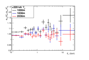
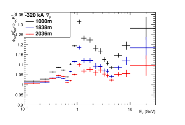
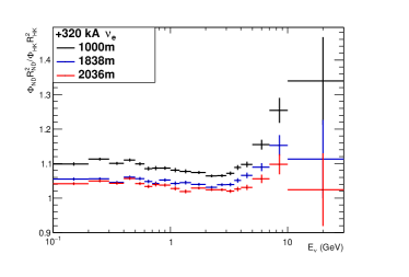
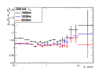
Figure 4: Flux ratios to the far detector normalised to the baselines for the $\nu_{\mu}$-enhanced beam (left) and $\overline{\nu}_{\mu}$-enhanced beam (right) for the different neutrino types. Errors are statistical only. The peaks, as seen in the top left and second-from-the-top right plots, are from the change in the ratio from the pion contribution to the flux. This is related to both the horn current and the solid angle subtended by the detectors with respect to the neutrino production points and hence is more prominent at a closer baseline.

The J-PARC accelerator delivers beam in discrete “spills”, each of which consists of a number of narrow “bunches”. Here we assume that the time between spills is 1.3 s and that each spill has a window of 1.3 $\mu$s, contains 8 bunches, and delivers $3.8\times 10^{14}$ protons-on-target, equivalent to a 1.3 MW beam. In addition, we assume that each bunch has a 1$\sigma$ width of 25 ns and that events occur within $\pm 50$ ns of the bunch [8]. The normalisation used for the neutrino fluxes for baseline and tank optimisation studies will be reported on a per-spill and per-bunch basis.

The ratios of the flux at each baseline compared to Hyper-K for each flavour, with the baselines taken into account, are shown in Figure 4. The baseline which has the least variation in the flux relative to the Hyper-K far detector for all neutrino flavours is at 2036 m, followed closely by 1838 m. The neutrino flux at 1000 m shows greater variation due to the fact that the beam is observed more as a line source than a point source as it would be at the far detector. This is independent of the neutrino flavour or the horn current. From Figure 4, it is apparent that a longer baseline is preferred for the physics goals outlined in section 2.

Baseline (m)	$\nu$-int./kT/spill	$\nu$-int./kT/bunch
1000	2.56	0.31
1838	0.73	0.09
2036	0.57	0.07

Table 1: Number of beam neutrino interactions on water per kiloton per spill or per-bunch for the $\nu_{\mu}$-enhanced beam configuration at different baselines. The calculation uses NEUT 5.3.3 for the cross section model.

In addition, the number of beam neutrino interactions on water per-kiloton per-spill was calculated using the fluxes described above, and NEUT [9] 5.3.3. These are shown in Table 1 for the $\nu_{\mu}$-enhanced, or forward horn current (FHC), beam configuration, which has a larger total event rate than the $\overline{\nu}_{\mu}$-enhanced, or reverse horn current (RHC), beam configuration. Table 1 shows that baselines at a distance of roughly 2 km have a lower, but sufficient, event rate of roughly one event per spill, which also implies lower probabilities of pileup.

4 Neutron capture with gadolinium

As discussed in section 1 gadolinium doping is used in TITUS to enhance the efficiency of neutron capture.

Even moderately energetic neutrons, with kinetic energies from tens to hundreds of MeV, will quickly lose energy by collisions with free protons and oxygen nuclei in water. The cross sections for these capture reactions are 0.33 barns and 0.19 millibarns, respectively, so to first approximation every thermal neutron is captured on a free proton via the reaction $n+p\rightarrow d+\gamma$. The resulting gamma has an energy of 2.2 MeV [10] and makes very little detectable light since any Compton scattered electron is close to the Cherenkov threshold. The entire sequence from liberation to capture takes around 200 $\mu$s, with only a very small dependence (plus or minus a few $\mu$s) on initial neutron energy.

The situation is much improved by adding a water-soluble gadolinium compound, gadolinium chloride, GdCl₃, or the less reactive though also less soluble gadolinium sulphate, Gd₂(SO₄)₃, to the water. Naturally occurring gadolinium has a neutron capture cross section of 49700 barns, and these captures produce an $\sim$8.0 MeV gamma cascade. The visible energy will be around 4–5 MeV in a WC detector. Due to the larger cross section of gadolinium, adding 0.2% by weight (about 0.1% Gd) of one of these compounds is sufficient to cause 90% of the neutrons to capture visibly on gadolinium. Following the addition of gadolinium, the time between neutron liberation and capture is reduced by an order of magnitude to around 20 $\mu$s, greatly suppressing accidental backgrounds.

The gadolinium neutron capture is an established technique for low energy physics such as reactor oscillation experiments [11]. The plan with TITUS is to extend this technique to physics around 1 GeV. The main motivation is that the nucleon multiplicity provides information about the primary interaction. This can be seen from the following reactions:

$\bullet$ $\nu_{\mu}$CCQE,  $\sim$ 0 neutron, $\nu_{\mu}+n\rightarrow\mu^{-}+p$
$\bullet$ $\nu_{\mu}$CC-npnh,  $\sim$ 0.3 neutron, $\nu_{\mu}+(n+p)\rightarrow\mu^{-}+p+p~{},~{}\nu_{\mu}+(n+n)\rightarrow\mu^{-}+n+p$
$\bullet$ $\bar{\nu}_{\mu}$CCQE,  $\sim$ 1 neutron, $\bar{\nu}_{\mu}+p\rightarrow\mu^{+}+n$
$\bullet$ $\bar{\nu}_{\mu}$CC-npnh, $\sim$ 1.7 neutron, $\bar{\nu}_{\mu}+(n+p)\rightarrow\mu^{+}+n+n~{},~{}\bar{\nu}_{\mu}+(p+p)\rightarrow\mu^{+}+p+n$

where the average number of neutrons is obtained using NEUT 5.3.3. We assume that the correlated nucleon pairs for the npnh interactions are dominated by neutron-proton pairs. Naïvely, we expect a different number of neutrons from different primary interactions, either neutrino or antineutrino, hitting single nucleon or correlated nucleons. This could be modified event-by-event by nuclear effects such as re-scattering, charge exchange, and absorption in the nuclear medium. Nonetheless, it is expected that the primary interaction information is statistically conserved[12].

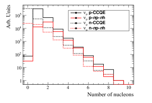
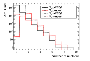
Figure 5: Number of protons and neutrons escaping from the target nuclei (water) with the CCQE or CC-npnh interactions after final state interactions. The top left plot is for muon neutrino interactions and the top right plot is for muon antineutrino interactions. The same information is shown on the bottom plots, but on a log scale.

Figure 5 shows the number of outgoing neutrons for different interaction channels that we expect to dominate for a particular beam horn current configuration. We used NEUT 5.3.3 to simulate the neutrino/antineutrino interactions with a water target. NEUT simulates the interactions with correlated nucleon pairs, on top of genuine CCQE interactions. In the figure, the different final states for $\nu$CCQE, $\bar{\nu}$CCQE, $\nu$CC-npnh, and $\bar{\nu}$CC-npnh display different neutron multiplicity spectra, indicating that this could be a new tool to identify the primary interaction in cases where standard water Cherenkov detectors cannot.

A comparable technology, the proton multiplicity measurement, is also under development by LArTPC [13]. These two nucleon-counting techniques are complementary, and new information about the outgoing nucleons will improve the performance of neutrino energy reconstruction, usually focused on the lepton kinematics, necessary to measure the CP violating Dirac phase in the lepton sector.

5 External background and pile-up

The external background consists of particles originating from sources other than neutrino interactions in the detector. They can be misidentified as a signal due to a reconstruction error or re-interaction inside the detector volume. We consider two possible sources of background: the interactions of beam neutrinos in the surroundings of the detector, which coincide with the beam window, and accidental cosmic rays. This section presents the methods used to estimate the background rate, leading to the optimisation of the detector design.

5.1 Sand interactions

Neutrinos from the beam interact not only in the detector, but also in the surrounding sand and pit structures. The particles coming from these interactions that enter the detector cannot be removed by cutting on the bunch time, because they produce signal in the same time as the interactions in the detector. These interactions will be referred to as “sand interactions” below.

Neutral particles coming from the sand interactions can re-interact inside the detector producing a false signal in the fiducial volume, whilst charged particles may be mis-reconstructed as starting inside the detector. Additionally, the sand events can pile up with the interactions in the detector. Particles from these interactions therefore lower the selection efficiency and purity.

A dedicated simulation allows us to predict the rate of these particles entering the detector. The simulation is performed in two steps.

First, the neutrino interactions are simulated with the NEUT generator (version 5.3.3). The neutrinos from the beam are allowed to interact in a rectangular volume filled with sand and positioned at the distance of 2036 m with respect to the target. The size of the volume is 100 m (L) $\times$ 40 m (W) $\times$ 40 m (H). There are no measurements concerning the chemical composition and density of the sand at the candidate TITUS sites, so it is assumed that the sand is pure SiO₂ with a density equal to 2.15 g cm^-3.

The next step is the propagation of particles produced in the neutrino interactions using the Geant4 package (version v9r4p04n00) [14]. The particles which reached the surface of a box big enough to encapsulate the water tank and the proposed MRD (23 m (L) $\times$ 13.86 m (W) $\times$ 12 m (H), see section 6.2) are saved for further propagation through the detector setup. The box is placed centrally inside the sand volume.

The primary particles are tracked through the sand until they enter the detector box, stop, decay or exit the geometry setup. Secondary particles produced in re-interactions are tracked as well, in the same way. However, not all the primary or secondary particles are propagated: low-energy particles produced at the distance of about 10 m from the detector have no chance of entering it and are therefore skipped to reduce the CPU time needed for the simulation. The cuts were tuned using a smaller sample to ensure that the final number of particles entering the detector box is not affected.

The numbers of particles entering the box are summarised in Table 2 for a generated sample of $2.5\times 10^{20}$ POT. Not all of them will enter the tank or MRD and produce a signal because they will not produce enough Cherenkov light to be detected or their direction is too close to the detector axis. Note that the total contribution of these particles will be given in the detector optimisation studies in section 6.1.

	Number of particles	Rate per spill
muons	375 615	0.33
neutrons	9 179 373	8.08
protons	45 885	0.04
charged pions	31 444	0.03
photons	3 046 799	2.68
electrons and positrons	214 878	0.19
other	2 233	0.002

Table 2: Number of particles of various types produced in the sand interactions and entering the detector box surface (see text for explanation). The second and third columns show numbers for the whole generated sample of $2.5\times 10^{20}$ POT, and the rate per spill of $2.2\times 10^{14}$ POT, respectively.

The most numerous particles are neutrons, which are mostly slow (about 75% have a momentum below 20 MeV/c). The momentum distribution for neutrons is shown in Figure 6 a).

Muons are essentially all produced directly in the neutrino interactions and as a result their energy is quite high. The momentum distribution, as shown in Figure 6 b), is peaked at about 200 MeV/c and 97% of muons have a momentum higher than that value.

Photons, electrons and positrons arriving to the detector are mostly (about 98%) produced in electromagnetic cascades produced by particles crossing the sand. There is also a small fraction of primary photons emitted from the target nuclei and electrons produced by interactions of electron neutrinos. The energy distribution of photons and the momentum distribution of electrons and positrons are shown in Figure 6 c) and d), respectively. The distributions are dominated by low energy particles: 90% of photons and 50% of $e^{\pm}$ have a momentum below 10 MeV/c.

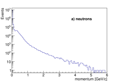
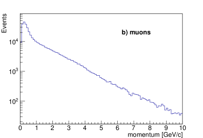
Figure 6: Momentum distributions for the a) neutron, b) muons, c) photons and d) electrons and positrons created in the neutrino interactions in the sand and entering the detector box for a whole generated sample of $2.5\times 10^{20}$ POT.

The particles that reach the surface of the box can then be further tracked by the detector simulation tool. The results are used in the tank optimisation and veto studies, described in section 6.1.

5.2 Cosmic background sources

Cosmic-ray muons and muon-induced spallation neutrons constitute additional sources of background. Both may cause events that coincide with the beam window, producing a non-beam- induced background. For the tank optimisation studies, we use the results from C. Galbiati and J.F. Beacom [15] at sea level, which are reported in Table 3. The cosmic ray muon background is reported in Table 3 as a flux (events per square meter per hour), whereas the neutron background scales with the detector water mass in kilotons (kT). Once these backgrounds are scaled to the 1.3 $\mu$s window of the neutrino beam, the cosmic-induced background contributes a negligible amount to the total event rate regardless of detector orientation or shape.

Depth (m)	$\Phi_{\mu}$	# of neutrons
	($\mu$m-2day-1)	(events kT-1 day-1)
0	$1.44\times 10^{6}$	$7.2\times 10^{6}$

Table 3: Cosmic muon flux, $\Phi_{\mu}$, and number of spallation neutron background events at sea level. Taken from [15].

6 Detector design

In this section we describe the different components of the detector. A detailed optimisation has been performed for the tank and the MRD. Realistic solutions for a WC detector with gadolinium doping are proposed for the electronics, DAQ, photosensors and calibration.

6.1 Tank

Detailed studies have been performed to optimise the size of the inner detector (ID), the tank orientation, the baseline, and the addition of an outer detector (OD), while taking into account the physics goals of the detector.

To optimise the tank size, we study both $\nu_{\mu}$-enhanced and $\overline{\nu}_{\mu}$-enhanced beam CC interactions at 2036 m, the preferred detector baseline, since these interactions provide the signal sample for the oscillation studies at Hyper-K. For each generated CC interaction, a vertex is randomly thrown in the tank muon from the interaction would generally be contained in the ID. From each point thrown in the detector, the distance to the tank wall along the direction of travel for the outgoing lepton is calculated as well as the energy loss assuming a constant loss of 1.981 MeV/cm [6]. The muon is considered contained in the ID if it has a non-positive kinetic energy when propagated to the tank wall.

Using the total event rate calculated from Table 4, tanks of different radius and length have been studied, and it is concluded that an ID of radius of 5.5 m and length of 22 m, corresponding to a water mass of 2.1 kT, has the desired performance. For an ID of this size, the overall fraction of muons contained as a function of their momentum and angle with respect to the beam that are contained is greater for a tank oriented along the beam than perpendicular to it, as shown in Table 5 and Figure 7. The 2.1 kT ID gives a similar number of events at 2036 m and 1838 m, as seen in the last column in Table 6. This shows that at a baseline of $\sim$2 km, the size of the TITUS ID does not need to undergo a re-optimisation. For a baseline of 1 km, due to the higher probability of event pileup, the TITUS ID volume should be reduced by roughly a factor of four, unless we introduce the Outer Detector, as we will see later in this section.

Baseline (m)	FHC	RHC
1000	2.56	0.87
1838	0.73	0.24
2036	0.57	0.19

Table 4: The number of beam neutrino interactions per kT per spill for a $\nu_{\mu}$-enhanced beam (FHC) and $\overline{\nu}_{\mu}$-enhanced beam (RHC).

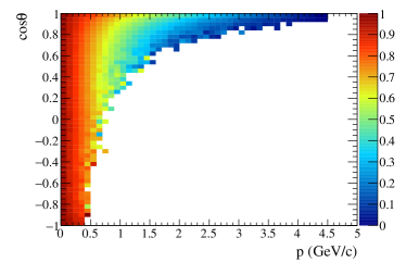
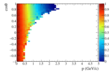
Figure 7: Fraction of muons that are fully contained in the nominal TITUS ID as a function of the muon momentum and angle with respect to the beam. The top(bottom) row shows $\nu_{\mu}$($\overline{\nu}_{\mu}$) interactions. The left column has the z-axis of the cylindrical tank along the beam direction while the right has a vertical z-axis.

Beam Type	% Contained Oriented Up	% Contained Oriented Along Beam
FHC	62.6	67.8
RHC	56.6	66.2

Table 5: Percentage of contained muons for the inner detector z-axis oriented up and along the neutrino beam direction for a $\nu_{\mu}$-enhanced beam (FHC) and $\overline{\nu}_{\mu}$-enhanced beam (RHC).

We then look at the expected rate from the beam and external background for the chosen tank (radius of 5.5 m and length of 22 m) with and without MRD and OD.

For the tank configurations and baselines we have considered only events that are in-time with the beam, which includes beam-induced interactions on water and, where applicable, iron, sand interactions, and cosmic sources. The event rates for water are taken from Table 4, the sand muon simulation is used to track particles to where they enter the tank and cosmic sources are calculated from Table 3. In each case, all water in the tank is assumed to be Gd-doped, so the neutron capture background can be considered for neutrons that will have a capture time nearly in-time with the beam. A fiducial volume cut is also applied to the event rates. The assumption is that the reconstruction can reasonably select events that have a reconstructed vertex at least 1 m away from the ID tank wall, giving a fiducial volume of 1.27 kT. This cut will be optimised as reconstruction improves, and is used here for illustrative purposes.

We study three possible configurations:

1. only a tank, where an outer detector (OD) of water surrounds the ID (similar to Super-K);

2. a tank and a downstream muon range detector (MRD), with an OD surrounding the rest of the tank;

3. a tank and an MRD that covers both the downstream face of the detector and 75% of the barrel, with an upstream OD of water.

Where the design includes an MRD, particles from iron interactions are tracked to see if any make it into the TITUS ID. The total number of beam neutrino interactions per spill in water for each of these studies and the TITUS ID is given in Table 6.

Baseline (m)	Study 1 (ev/spill)	Study 2 (ev/spill)	Study 3 (ev/spill)	ID (ev/spill)
1000	8.13	7.80	5.60	5.34
1838	2.31	2.20	1.58	1.51
2036	1.84	1.75	1.27	1.20

Table 6: The number of beam neutrino interactions per spill for a FHC beam configuration in the TITUS tank and ID for detector designs with no MRD (1), downstream MRD only (2), and downstream plus barrel MRD (3); see text for further details. The final column are the number of beam neutrino interactions per spill just in the ID, which is a subset of the events in each of the first three columns.

Baseline (m)	Tank ev/spill	Tank ev/bunch	ID      ev/spill	ID ev/bunch	FV ev/spill	FV ev/bunch
1000	67.89	8.44	6.79	0.81	4.17	0.49
1838	19.40	2.37	2.17	0.24	1.37	0.14
2036	15.44	1.89	1.80	0.19	1.20	0.12

Table 7: The number of interactions per spill and bunch, assuming a SK-style OD, in the whole tank, the ID, and a possible fiducial region (FV).

In the case where there is no MRD as part of the TITUS complex, the ID is surrounded by an additional layer of water, similar to the Super-K design. The OD depth is 1 m giving the tank dimensions of 6.5 m in radius and 24 m in length corresponding to a total water mass of 3.18 kT. The event rates per spill and per bunch assuming a $\nu_{\mu}$-mode beam for the whole tank and the ID are given in Table 7. It is assumed that all Cherenkov particles in the OD are vetoed. Neutrons with a kinetic energy $T_{n}<10$ MeV are considered captured in the OD, since they have a range less than 1 m, and all neutrons with $T_{n}<20$ MeV are captured before entering the fiducial region.

Baseline (m)	Tank ev/spill	Tank ev/bunch	ID      ev/spill	ID ev/bunch	FV ev/spill	FV ev/bunch
1000	67.65	8.35	7.14	0.81	4.40	0.50
1838	19.31	2.36	2.17	0.24	1.44	0.14
2036	15.37	1.87	1.87	0.19	1.20	0.12

Table 8: The number of interactions per spill and bunch assuming a downstream MRD and the rest of the tank surrounded by a SK-style OD in the whole tank, the ID, and a possible fiducial region.

For the case where there is only a downstream MRD, we assume that there is the equivalent of 0.5 m of iron used in the detector to track the possible particles in the tank. The MRD itself is assumed to be circular in this study, though more details will be given in section 6.2. The rest of the ID is again assumed to be surrounded by 1 m of water, giving a total water mass of 3.05 kT. It is also assumed that none of the sand interactions enter from the region covered by the MRD. The event rates are given in Table 8.

Baseline (m)	Tank ev/spill	Tank ev/bunch	ID      ev/spill	ID ev/bunch	FV ev/spill	FV ev/bunch
1000	17.09	1.80	8.61	0.74	5.65	0.46
1838	5.06	0.50	2.69	0.23	1.78	0.14
2036	4.09	0.40	2.21	0.17	1.47	0.10

Table 9: The number of interactions per spill and bunch assuming a downstream and barrel MRD and upstream of the tank surrounded by a SK-style OD in the whole tank, the ID, and a possible fiducial region.

Finally, the event rates for the case with a MRD covering both 75% of the TITUS barrel and the downstream region and a 1 m OD upstream of the TITUS ID are computed. The remaining region around the barrel is assumed to have a neutron absorbing material, e.g. boron-doped polystyrene, to further reduce the possible number of neutrons entering the tank. An additional veto is assumed to be placed between the polystyrene and the TITUS tank to veto particles created in the material that may enter the tank. The event rates are given in Table 9. The earlier conclusion on detector location based on pile-up rates is independent of the detector configuration.

Based on the above studies, the area around the ID not covered by the MRD needs to have 1 m of water between the external wall of the tank and the optical separation between the OD and ID. This is to act as a neutron shield for the ID due to incoming neutrons from interactions in the surrounding material, veto charged particles from interactions in the OD or outside the detector, and to determine if particles from interactions in the ID deposited all their energy in the ID, or if they exited.

The MRD design in section 6.2 complicates a Super-K style OD in that some space needs to be cut out in the middle of the barrel to accommodate a small MRD. The overall tank design must take this feature into account. For both the downstream and barrel components, the area of the MRD that faces the tank must have at least one additional layer of scintillating strips to identify charged particles entering or exiting from the MRD into the tank.

6.2 Magnetised muon range detector

Outside the TITUS tank a magnetised iron tracking detector with a 1.5 T field is proposed. This serves to range out muons and measure their momentum and charge. It complements the water Cherenkov detector by both increasing the sample size and directly constraining the “wrong-sign” components in the $\nu_{\mu}$ and $\bar{\nu}_{\mu}$ beams, which are an important source of uncertainty in super-beam measurements of CP violation. However, a correction to the susceptibility caused by the paramagnetic nature of the Gd₂(SO₄)₃ will be applied. The correction depends on the temperature. At about 12°it is around 0,4%.

The design, which is illustrated in Figure 8, includes a full downstream magnetised muon range detector (MRD) and a small magnetised side-MRD. The diameter of the downstream magnetised MRD matches that of the tank (13 m including both ID and OD) and has a thickness of 2 m, allowing the forward scattered muons which escape the tank to be included in the oscillation fit up to a momentum of 2 GeV/c. The smaller side-MRD has dimensions of 4 m$\times$7 m with a thickness of 2 m, and is also magnetised, allowing a measurement of the less well understood high-$Q^{2}$ region of phase space. This region may be useful for testing and discriminating between neutrino interaction models, and should help with the wrong sign measurement in antineutrino mode, since the muons have different angular distributions for $\nu$ and $\bar{\nu}$ interactions.

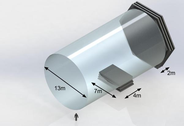
Figure 8: The proposed configuration of the magnetised muon range detectors of the TITUS experiment. A large magnetised MRD with radius 13 m to match the Cherenkov tank and thickness 2 m, is placed downstream of the tank, to measure the momentum of forward-going muons. A smaller magnetised side-MRD is placed on the side of the tank to allow low-background measurements of the antineutrino cross-section in this high-angle region of phase-space.

Tracking muons in magnetised iron is a well-established technique which has been successfully employed in several experiments (e.g. [16]) where charge reconstruction efficiencies are typically in the range 95% – 98%. The design of the TITUS magnetised MRD features 6 cm thick planes of iron interleaved with orthogonally arranged pairs of scintillator planes which sample the position of particle tracks. The magnetised MRD will measure the momentum and total energy of muons leaving the water volume, up to a range-out momentum of 2 GeV/c. The high position resolution of the scintillator plates (1 cm) will enable precise measurements of the curvature and a strong, well-understood particle identification (PID) via the direction of curvature.

To provide a 1 cm spatial resolution highly segmented scintillator detectors consisting of scintillator bars with wavelength-shifting (WLS) fibers and Multi-pixel Geiger mode avalanche photodiodes as photosensors are considered as a realistic option for active elements of the MRD. The real challenge lies in the required fine granularity and size of the scintillator detectors for the MRD. Each individual element should have good characteristics to detect minimum ionising particles (MIPs) with high efficiency in such a large detector system. A detector option, successfully realised in ND280, is based on 7-10 mm thick extruded polystyrene scintillator bars with WLS fibers embedded with an optical glue. The length of the bars covered by a chemical reflector by etching the scintillator surface in a chemical agent can be up to 8 meters. For the readout, 1 mm Kuraray Y11 WLS fibers can be applied. The results of the tests long extruded bars are presented in Ref. [17]. It is important to stress that even 7 mm thick very long detectors (length of 16 meters) provide a light yield of 16 photoelectrons per MIP and more than 99% efficiency for detection of MIP’s. It should be noted that the time resolution of about 2 ns can be reached for these detectors. Shorter scintillator detectors will be needed for a smaller magnetised side-MRD placed on the side of the tank. In this case, the light yield of 60 photoelectors/MIP and time resolution of $\sigma=0.7$ ns was obtained for detectors of about 3 m long [18]. This good performance allows us to instrument both the MRD’s with such detectors.

Higher energy muons ($p_{\mu}\gtrsim 1$ GeV/c) will travel through many iron planes and their charge can be measured with very high efficiency by reconstructing their curved trajectories in the 1.5 T magnetic field inside the iron. This sample is particularly interesting with regard to the validation of the complementary gadolinium charge reconstruction technique. This novel technique, described in section 4, is powerful as it can be applied to all events, but the MRD can be used to both calibrate the neutron capture and provide a more precise measurement of the charge separation.

A measurement of the efficiency of the gadolinium technique using the high energy MRD sample will allow us to exploit its full potential. The mean charge reconstruction efficiency for all events in the downstream MRD is estimated to be 95%. Furthermore, the precise calibration of the performance of the gadolinium charge reconstruction in TITUS will be greatly advantageous if it is used in the far detector, Hyper-K, or indeed in other neutrino experiments, as it will help in minimising the neutrino interaction modelling systematic error.

The most interesting sample of muons is those resulting from neutrino events near the oscillation maximum at $E_{\nu}\sim 0.6$ GeV. The muon charge is more difficult to reconstruct using the traditional method as the tracks may traverse only a handful of planes. The design has therefore been optimised for the lower energy muon spectrum of Hyper-K using a novel arrangement of the first three iron planes by the introduction of double scintillator planes and 10 cm air gaps, both of which increase charge reconstruction efficiency for short tracks. In this case one does not fit tracks, but rather measures the angle of the particle trajectory before and after each iron plane, and observes the direction of curvature. This technique is ultimately limited by multiple scattering; however, several such measurements will allow an efficiency of 90% for events at the oscillation peak, a figure which is comparable with the efficiency expected from the independent gadolinium measurement. When these two methods are combined it will be possible to obtain $\sim 96$% pure $\nu_{\mu}$ and $\bar{\nu}_{\mu}$ samples from events in the oscillation peak in TITUS.

The principle for this detector is being optimised at the University of Geneva through the Baby-MIND detector [19] which is conceived as a proof of principle of low energy charge reconstruction using magnetised iron. It has been shown that the detector can be magnetised using aluminium coils which do not reduce the reconstruction efficiency and require minimal power to operate. This design is discussed in detail in [19]. It has been accepted as part of the WAGASCI experiment [20].

This will be a valuable proof of principle for the TITUS MRD. The design of the side-MRD is the same as that of the Baby-MIND, but with increased transverse dimensions of 4 m $\times$ 7 m, allowing the coil arrangement to be the same.

In addition to constraining the wrong-sign component, the MRD will measure the momenta of muons leaving the water tank by ranging them out in the iron in the traditional fashion. In the nominal TITUS design, 18% of the muons exit the tank, with a preference for the forward direction. This number is much greater than in the far detector due to the necessarily limited size of any intermediate detector. Without an MRD these events would be excluded from the oscillation analysis. The MRD therefore also gives a statistical benefit of over 10%, allowing muons which escape the tank to be included in the analysis.

6.3 Photosensors

TITUS will contain over 3000 photodetectors and their performance is critical for the success of the experiment. Excellent temporal and spatial resolution is required in order to precisely determine the vertex position of each CCQE interaction. The default configuration for TITUS, assumed in all studies unless otherwise stated, uses 12” photomultiplier tubes (PMTs) with the same quantum efficiency as the 20” Hamamatsu Type R3600 PMTs currently used by Super-K, but with flat rather than hemispherical morphology of the glass. However, several alternative photosensor technologies may offer improved performance and are currently under study. In this section we present status reports on hybrid PMTs that have the advantage of lower cost, multi-PMTs and Large Area Picosecond PhotoDetectors (LAPPDs).

6.3.1 Hybrid photosensors

We have investigated the latest 8” hybrid photomultiplier tube (HPD) developed by Hammamatsu, the R12112. These devices use an avalanche photodiode instead of dynodes to achieve high single photon sensitivity and good time resolution. The 20” equivalent of this PMT is being considered as a possible candidate photosensor for the Hyper-K far detector. The R12112 has a bi-alkali photocathode and is specified to have a quantum efficiency of 27.2% at 380 nm. At 10 kV the gain is $10^{5}$ with a dark current of 20 nA.

A photosensor test system is currently being installed in the laboratory at the University of Edinburgh. Single photon signals can be generated either by cosmic muons passing through a 10 mm quartz plate mounted directly above the HPD or by a pulsed LED source. Figure 9 (left) shows the amplified signal from the HPD when using the pulsed LED source while Figure 9 (right) shows the spectrum of analog-to-digital converter (ADC) channels recorded by the data acquisition system when triggering on cosmic muons. The single-photon peak is clearly visible above ADC channel 100. Work is ongoing to further optimise and calibrate the HPD testing facility. Further measurements will be carried out, including a test of the effect of magnetic fields on these devices.

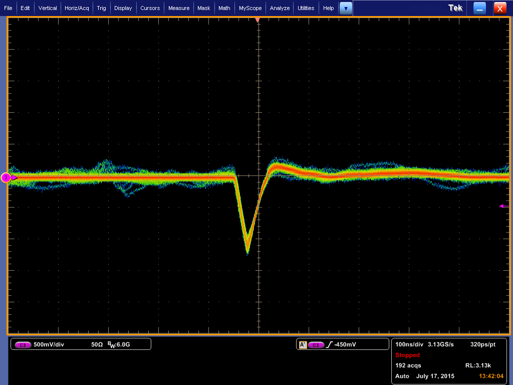
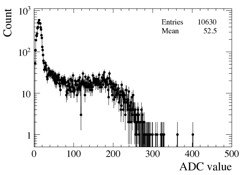
Figure 9: (Left) Oscilloscope trace of R12112 photodetector signal in response to pulsed LED light source inside the testing station. HV and LV control voltages were set to 2.5 V and 1.2 V, respectively. (Right) Spectrum of ADC channels from a test HPD when triggering on cosmic muons.

6.3.2 Multi-PMTs

An interesting option for the photodetector system is based on the multi-PMT digital optical modules (DOMs) used by the Km3NeT experiment [21].

The detection element of the KM3NeT deep-sea Cherenkov detector is a pressure resistant glass sphere that contains photomultipliers, with dedicated electronics, embedded in a transparent silicone gel to ensure mechanical and optical coupling [21]. A photograph and schematic diagram of the KM3NeT multi-PMT DOM is shown in Figure 10.

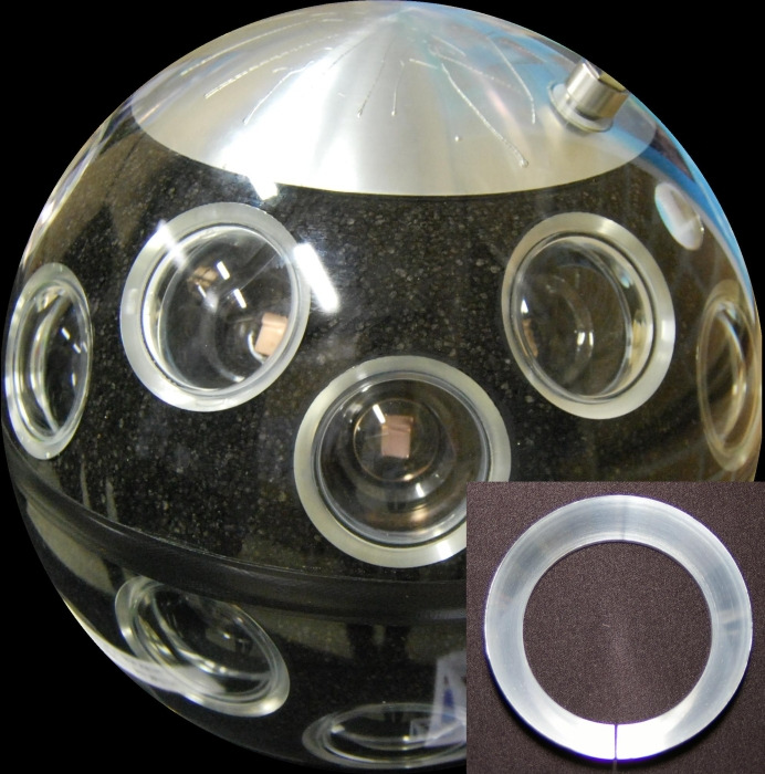
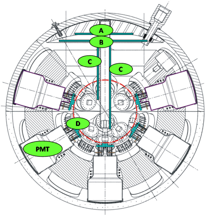
Figure 10: (Left) A mechanical reference model of a multi-PMT DOM with reflectors surrounding 3” PMTs. (Right) Schematic drawing of a multi-PMT DOM; D: PMTs including their bases; A: aluminium cooling structure; B and C: front-end electronic components [22, 23].

This design has various advantages compared to traditional optical modules with a single large PMT [24, 25]. In particular, while the total photocathode area is the same or even larger than in the case of a single large PMT, there is an increase in segmentation of the photocathode area that will help in distinguishing single-photon from multi-photon hits, resulting in an efficient background rejection with a low background rate even at the single DOM level. Indeed, two-photon hits can be unambiguously recognised if the two photons hit separate tubes, which should occur in 85% of all cases. In addition, adjacent tubes can be selected to enhance the signal coming from a single direction, whereas the background is mostly randomly distributed [26]. Thus, the arrival of more than one photon at the DOM is identified with a high efficiency and purity and provides a sensitivity to the direction of the detected light.

The reliability of the multi-PMT DOM is high, since the failure of a single PMT should minimally degrade the performance of the photodetector system.

The preliminary design assumes a hemispherical multi-PMT DOM with seven 3” PMTs, one on the top of the hemisphere and the others arranged on the vertices of a hexagon. The choice of small PMTs is based on the possibility of having a quantum efficiency above 30%, a small transit time spread, no need to shield from the Earth’s magnetic field and lower cost. The baseline option is the same as the 3” PMT used in KM3NeT [26], but an innovative small surface area hybrid photodetector can also be considered (see for example [27]).

The vessel is important to protect the photomultipliers and associated equipment against the hydrostatic pressure and water. In KM3NeT commercially available borosilicate glass spheres are used for the vessels. Earlier studies from the KM3NeT Collaboration indicated that sources of noise in the optical module include light produced either by the scintillation or Cherenkov effect or by radioactive contamination (⁴⁰K) in the glass material itself [28]. This background can be reduced in TITUS by using a custom-built acrylic pressure vessel. Several studies are ongoing to choose the best shape and material.

Detailed simulation will be needed to determine the optimal design and the best PMT choice for TITUS detector.

6.3.3 LAPPDs

An attractive alternative photosensor, though not yet commercially available, is the Large Area Picosecond PhotoDetector (LAPPD) [29]. The LAPPD is an imaging detector based on micro-channel plate (MCP) technology, with a $20\times 20$ cm tile basic layout, shown in Figure 11 (left). It is able to resolve the position and time of single incident photons within an individual sensor. This maximises the use of the fiducial volume as it permits the reconstruction of events very close to the wall of the detector, where the light can only spread over a small area. Preliminary Monte Carlo studies indicate that the measurement of Cherenkov photon arrival space-time points with resolutions of 1 cm and 100 ps will allow the detector to function as a tracking detector, with track and vertex reconstruction approaching size scales of just a few centimetres [30]. Imaging detectors would enable photon counting by separating the space and time coordinates of the individual hits, rather than simply using the total charge. This means truly digital photon counting and would translate directly into better energy resolution and better discrimination between dark noise and photons from neutron capture with a time resolution better than 100 ps and a spatial resolution of the order of 3 mm for single photons. The design of the LAPPD is based on low-cost materials, well-established industrial techniques and advances in material science.

This technology is still in development and the number of available tiles is limited. The ANNIE (Accelerator Neutrino Neutron Interaction Experiment) experiment at Fermilab [31] aims to be the first neutrino experiment to test the tiles when available. This will allow the benefits of imaging photosensors to be understood. Small $6\times 6$ cm prototype MCP tiles using a similar technology have been obtained by the Edinburgh and Sheffield groups from Argonne Lab [32] and tests are being made in the laboratory to understand the performance of these devices, in particular in a magnetic field. Figure 11 (right) shows an example oscilloscope trace when the test LAPPD is illuminated with an LED source.

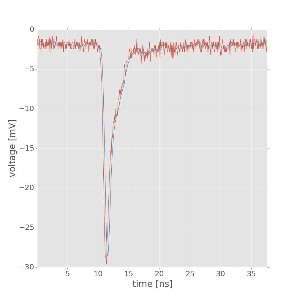
Figure 11: (Left) Schematic view of the LAPPD tile. (Right) Oscilloscope trace of a single photon single from a MCP tile in the Edinburgh test facility. The red line is the raw signal, the blue is after digital filtering.

6.3.4 Photosensors for MRD

The MRD detector will consist of a large number of scintillator detectors and therefore will have a large number of readout channels that require the usage of very compact, insensitive to magnetic field photosensors with a high sensitivity to the green light emitted from WLS fibres. Multi-pixel Geiger mode avalanche photodiodes are recettly used as photosensors in such detectors. Detailed information about these photodiodes and their basic principle of operation can be found in Ref. [33]. The first application of Geiger mode avalance photodiodes in a large-scale experiment has been done in the near neutrino detector ND280 [34] of the T2K experiment where approximately 56000 Hamamatsu Multipixel Photon Counters (MPPCs) [35] are used.

Manufacturers have advanced in developing new generations of multi-pixel Geiger photodiodes referred as SiPMs in recent years. Various new SiPM types were developed by different companies (Hamamatsu, KETEK, SensL, AdvanSiD). The performance of Hamamatsu MPPC’s was greatly improved since 2009 when the ND280 was commissioned. The dark noise rate per mm² of active area was reduced by more than 10 times. The significant decrease of the dark noise enables us to operate the new MPPCs with higher over-voltage to achieve higher gain and this regime is relatively immune to temperature changes. The optical crosstalk and after pulses were significantly suppressed from the level of 10-20% to less than 1% that allowed to operate with lower level signals in scintillator detectors. The photon detection efficiency of new devices was also increased by about 2 times. The detailed study of new Hamamatsu MPPC’s and their parameters can be found in Ref. [36]. All these improvements are very important for applications of MPPC’s in large size detectors like the TITUS MRD.

6.4 Electronics and readout

To read out the 3000+ PMTs of the TITUS Cherenkov detector, we propose a trigger-less readout system based on well-established waveform digitising technology (WFD). The signals from the PMTs will be continuously sampled using flash ADCs operating in the GHz range with 12 to 14 bit resolution. The WFD technology combines in a single device traditional operations like constant fraction discrimination for timing, peak sensing and charge integration for energy measurements, etc. The advantage of this technology is that critical decisions on whether to read out events can be delayed until the whole waveform can be used to select interesting events PMT by PMT. Another advantage of this technology compared to traditional constant fraction discriminators and Time to Digital Converters (TDCs) is that pile-up can be effectively recognised and corrected for, with double hit resolution of the order of the rise-time of input PMT signals, permitting in principle, an individual measurement of each Cherenkov photon reaching the PMT.

The electronics design for TITUS needs to accommodate fast sampling of the Cherenkov light from the muon tracks ($\sim 100$ ps resolution over 100 ns duration) over the whole 5 $\mu$s spill, the Michel electrons, and the delayed capture of the thermal neutrons, which occurs approximately 30 $\mu$s later, as illustrated in Figure 12.

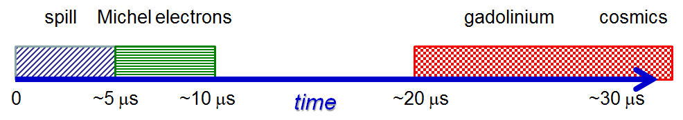
Figure 12: Diagram showing approximate arrival times of Cherenkov light from muons, Michel electrons and neutron capture, relative to the spill window.

The digitising electronics can be located close to the PMTs or several 10 m away. In both cases we consider using a differential transmission line using cat VI network cables. The single ended output from the PMT will be converted to a differential signal using high frequency RF transformers. The advantage of adopting RF transformers is that the ground of the PMT (including the HV base and possible preamplifiers) will be fully decoupled from the readout electronics ground. With PMT gains around $10^{7}$ there is no need to further amplify the PMT outputs, whereas if HPDs are used, a preamplifier will be required. On the other end of the transmission line, the differential PMT signal will be received by a large bandwidth amplifier which will also condition the signal before feeding it into the flash ADC.

All the readout chain is based on commercially available components used in the telecommunication industry. There are several commercially available flash ADC operating with 1 GHz sampling frequencies and 12 or 14 bit resolution. The flash ADC will be coupled to a high performance Field Programmable Gate Array (FPGA), also operating in the GHz range. Several flash ADCs can be driven by the same FPGA. The whole system will be synchronised using external clocks, operating in the MHz range, to which on board clock frequency multipliers will be phase loop locked (PLL).

Different waveform processing algorithms can be run in the FPGA. In the first stage, these algorithms will be used for baseline subtraction and zero suppression, etc. Next, different constant fraction discriminator algorithms can be used to extract the timing information from the waveforms. With a sampling frequency of 1 GHz a timing resolution better than 50 ps can be expected using fine-tuned algorithms. Further, charge-integrating algorithms can be used to determine the charge of the input pulse. Given that the signal duration is of the order of several tens of ns, the signal is sampled several times, so that the final ADC resolution will be higher than the resolution of the flash ADC (roughly $1/\sqrt{N_{\mbox{\scriptsize{samples}}}}$).

The drawbacks of this design are the cost and the considerable power consumption (3 to 5 W) per channel due to the high sampling frequency of ADCs, the high performance FPGAs operating in the GHz range and large bandwidth amplifiers. While the cost is not a serious issue (10 to 15% of the cost of a 20 inch PMT), especially for a near detector with a small number of PMTs, the power consumption can become an issue for large systems comprising up to 100,000 PMTs. The electronics industry is constantly developing new components (better performance, cheaper, lower power consumption) and the latest products will be used for the construction of the readout electronics.

The trigger and readout electronics will be developed jointly by the University of Geneva (UniGE), Queen Mary University of London (QMUL), et al. UniGE has significant prior experience with data acquisition systems and the development and implementation of fast WFD systems (NA61/SHINE experiment at CERN, MICE at RAL). QMUL also has significant expertise from work in the T2K and SNO+ experiments.

To reduce the power dissipation (and cost) one could consider using flash ADCs with lower sampling frequency coupled to lower performance FPGAs. For instance, one could consider splitting and phase shifting the input signal into a 4 ch. 250 MHz flash ADC, for an effective 1 GHz sampling frequency of the input signal, without any loss in performance but lower overall power dissipation.

An interesting option, particularly as regards lowering power consumption is to use circular switched capacitor arrays (SCA), which sample and store the waveforms into a capacitor array with a several GHz sampling frequency. The stored charges in the capacitor array are then digitised at a much lower frequency, around 50 MHz. UniGE has significant experience in developing and using digitising electronics using the DRS4 SCA developed at PSI [37]. The potential disadvantage of this solution based on the DRS4 SCA is the time required to read out the capacitor array (at least 15 $\mu$s), i.e. the dead time during which the SCA is not able to sample input signals, and the finite depth of the capacitor array ($\sim 10$ $\mu$s at 1 GHz sampling frequency). To solve this readout / deadtime issue, which could be of a problem for observing the delayed neutron capture, we will run several SCAs in parallel for the same input signal. As soon as one SCA is full and being readout, the sampling of the signal continues on the following SCA. In this way, there is virtually no deadtime in the system. Indeed, in a special operation mode, the DRS4 chip can also sample the input with one channel while reading out another channel at the same time, with slightly increased noise. This mode can be used to build a system with up to eight parallel analog buffers and with virtually zero dead time for event rates below the typical readout time (up to 500 kHz).

A new version of the capacitor array, the DRS5, is under development and expected for Summer 2016. Instead of storing the sampled waveform in a linear array, the waveform will be stored in a two-dimensional array (matrix) consisting of short waveform segments. The design of the chip is such that each segment can be read out individually, instead of the full array as for the DRS4. Instead of digitising the whole waveform, only interesting parts of the waveform would be digitised, making it an almost deadtimeless system and overcoming the limitations of the DRS4 ASIC. Four to eight such segments would typically be required to digitise an entire 100 ns PMT pulse, allowing a continuous acquisition rate of up to 500 kHz. As soon as this new ASIC is available, UniGE will start testing its performance.

6.5 DAQ

The Data Acquisition (DAQ) systems for the TITUS detector will collect raw (digitised) data output from the electronics and write formatted data to storage for offline analysis.

The data rate that the DAQ must support depends on the trigger strategy, which will be designed to store all interesting physics processes, discard non-physics events and provide reliable data storage onsite. Interactions in the TITUS detector will have energies ranging from a few MeV to several GeV. Beam events may be selected by an external trigger, if that is available. Alternatively, a simple N_hits threshold can be applied to select interactions that should be stored to disk. N_hits is defined as the number of WFD-identified peaks from PMT waveforms in a given time period; if the number of firing PMTs is greater than a pre-determined number threshold, the event will be read out. Cosmic ray interactions may be selected by a similar N_hits trigger or even with a random trigger given the high rate of cosmic muons in the detector (4 kHz from Table 3).

The acquisition window should be long enough to catch neutron captures; because these happen with an average delay of 30 $\mu$s since the primary vertex, a window of at least 300 $\mu$s should be chosen. Assuming for instance one cosmic ray trigger is issued in between every pair of beam triggers leads to the event rates collected in Table 10. Thus the DAQ system must be capable of supporting instantaneous event rates of order 50 GB/s and average rates of few MB/s.

Event rates
event type	$n$ hits in one DAQ window	instantaneous rate	average rate
beam neutrino	3982	0.77 GB/s	0.18 MB/s
cosmic muon	17669	3.4 GB/s	2.7 MB/s
PMT dark noise	15120	2.9 GB/s	1.3 MB/s
$\mu$ sand events	1314	0.25 GB/s	0.059 MB/s
$n$ sand events	420	0.081 GB/s	0.019 MB/s
214Bi in PMT	875	0.17 GB/s	0.078 MB/s
208Tl in PMT	131	0.025 GB/s	0.012 MB/s
total	39512	7.6 GB/s	4.4 MB/s

Table 10: Instantaneous and average data rates for different event categories. The numbers are obtained assuming that: the detector is instrumented with 6000 PMTs; each waveform is digitised in 30 samples, resulting in 58 bytes per hit; each PMT has a dark noise rate of 8.4 kHz; the glass of each PMT is contaminated with 27 Bq of ²¹⁴Bi and 2.8 Bq of ²⁰⁸Tl as was measured for the SK PMTs, and each of those decays generates respectively 18 and 26 hits on average; and finally beam and cosmic ray triggers are taken in alternation.

In the event of a supernova, it will be beneficial to read out the whole detector without zero-suppression for a number of seconds. For a supernova at a distance of 10 kpc, $\mathcal{O}$(300) neutrino interactions are anticipated in a $\sim$10 s time frame (see Table 27), leading to an average raw data rate of $\sim$0.3 MB/s. This is however a tiny perturbation of the total detector rate and cannot be triggered upon with the N_hits technique; the supernova could only be recognised by identifying the double presence of positron hits and delayed neutron capture hits or by an external trigger from SNEWS if the the DAQ has a buffer.

The DAQ system will use a number of custom front-end applications interfaced with an open source or custom-built framework, which will allow user operation via a web interface. It is anticipated that the same framework will be used by the Hyper-K and TITUS detectors. The DAQ will operate on commercially available computing hardware.

Monte Carlo simulations are currently being used to assess the performance of potential trigger algorithms, to calculate event rates, to determine the impact of system latency and to verify whether full digitization of pulse shapes is required. Results from such studies are being used to help define whether the trigger should be implemented in hardware or in a software farm.

A hardware-based trigger, as shown in Figure 13, would merge information from a group of PMTs on a “receive card” and data from several receive cards would be merged on a daughter card. Each daughter card would send N_hits information onto a trigger processor board; if the number of PMTs firing in an event exceeded a given N_hits cut, the event would be saved. If the number of hits was not sufficient, a sub-N_hits trigger would be activated in the electronics firmware of each daughter card. One way this could be implemented is to use the FPGA logic to divide the detector into smaller cells e.g. 500 cells containing a given number of PMTs. Each cell would have a look-up table of fixed time offsets for each PMT within it. The FPGA would look for coincidences in offset-corrected PMT times in a specific time window, in a given cell location in the compartment. A local N_hits threshold would be applied to each cell and, if at least one cell passes this requirement, the whole event would be written to disk.

In a software trigger system, as shown in Figure 14, all hits would be transmitted from the electronics to the DAQ and decisions on which time windows to keep would made in a farm. Data from a group of PMTs would be collected by a receive card, which would be connected to a large ethernet switch. The outputs of the switch would be connected to a processing farm of Linux machines or graphical processing units or similar. These processing nodes would see data from the entire detector, divided into time windows. Fast algorithms would be implemented on these processing nodes and decisions regarding whether to write the event to storage would be made at this point. Algorithms using spatial and time information are currently being developed.

Distributed cluster technology will be used for the DAQ and trigger farm, such that if one node fails, its processes automatically run on another node. This would allow faulty computer hardware to be exchanged with minimal impact on data taking. The computer cluster design is currently flexible until the final DAQ design and hardware choices are made.

Figure 13: Block diagram of a DAQ system with a hardware-based trigger. The paths of data and triggers are shown with the solid grey arrows and dashed red arrows respectively. N_hits triggers are created on the trigger processor board, and sub-N_hits triggers are created on the daughter cards; both are distributed by the trigger processor board. The numbers of daughter cards, receive cards, and PMTs have been reduced for clarity.

Figure 14: Block diagram of a DAQ system with a software-based trigger. The path of data is shown with the solid grey arrows. Triggers are created on a processing farm node, and read out to the standard DAQ backend. The numbers of processing farm nodes, receive cards, and PMTs have been reduced for clarity.

6.6 Calibration

In order to reduce the systematic uncertainties of TITUS to the level required by Hyper-K, it will be essential to thoroughly calibrate the TITUS detector. This will be performed using two calibration systems: one integrated light source and a deployment system for a variety of radioactive calibration sources.

A full calibration of the TITUS detector involves several individual sub-tasks: calibration of the PMT array, measurement of detector response parameters, and determination of the neutron detection efficiency. To calibrate the PMT array, the absolute time of each PMT with respect to the rest of the array must be measured, the dependence of the time on the deposited PMT charge must be determined for both single and multiple photon scenarios, and the charge response of the PMT to photons must be determined. The detector response parameters include the extinction and scattering of light in the water as a function of wavelength, any dependence of the PMT response on angle, and the overall detector gain. Finally, as TITUS uses Gd doping to increase sensitivity to neutrons, the neutron detection efficiency must be determined as a function of position in the tank. These needs can be met by the two calibration systems described below.

6.6.1 Integrated light source system

TITUS will include an integrated light source system for all optical and PMT calibrations. This system consists of a number of light injection points connected via optical fibres to light pulsers in the electronics. Light pulses of 1–2 ns can be produced relatively inexpensively using LEDs or similar solid state optical devices allowing multiple optical sources to be deployed around the edge of the detector. This system consists of an LED coupled to an optical fibre, which is then connected to an optical diffuser on the PMT support of TITUS. The optical diffuser is used to shape the light inside TITUS and a number of designs are possible, providing different calibration pulses for different needs. The key challenges are the coupling of the LEDs to the optical fibre, minimising dispersion in the fibre to maintain short optical pulses and achieving the required dynamic range. There are two points at which the light produced can be monitored, and TITUS will use both. First, the optical coupling between the LED and the fibre can be monitored by a solid-state device such as an MPPC or photodiode built into the LED-fibre coupling system. Second, a return fibre from the optical diffuser can also be implemented. These two systems will enable both pulse-by-pulse and long-term monitoring of the light entering the detector, allowing PMT and optical calibration data to be taken without the manpower-intensive calibration source deployment previously used in water Cherenkov detectors. These data can be collected either in dedicated high-rate calibration runs or interspersed during normal data-taking.

The calibration of the PMT timing requires a short duration light pulse of known origin and time. The integrated calibration system, from any given fibre, provides this but clearly cannot illuminate the entire PMT array at once. To minimise the number of fibres required the optical diffuser for the PMT calibration must provide a wide opening angle, of order 30 degrees, to illuminate a significant number of PMTs on the far side of the detector. The diffuser must be carefully designed to ensure that there is no time dependence as a function of angle. To achieve the overall calibration of global time offset of the array, PMTs must be illuminated by at least two fibres to allow the fibre times to be cross calibrated. For TITUS, four-fold degeneracy of the PMT calibration fibre points is the target to permit improved cross calibration and redundancy against single point failures in the fibres. This system will enable the calibration of PMT timing, the dependence of time on charge and the PMT time response.

The integrated calibration system can also be used to measure optical scattering, extinction and the PMT response. While the basic elements of the system are the same as that used for PMT calibration, a number of changes are required meaning that fibres and diffusers used for these calibrations are different. These properties must be measured as a function of wavelength, thus several LED types will be used to provide light at 6 different wavelengths between 330 nm and 500 nm. To measure scattering a narrow beam is required from the optical diffuser; the scattering length is measured by monitoring the light level of PMTs outside the narrow beam as a function of the path length of the beam through the detector. Optical extinction is measured by monitoring the light levels at specific PMTs inside the optical beams; unlike scattering, wide-angle beams are important for this calibration to provide a variety of path lengths. The pulse by pulse monitoring of the calibration system is essential for this calibration as the light level at given PMTs is the key measurement of the system. The measured light level at the PMTs is a combination of extinction and PMT response as a function of angle; several light paths and angles are needed for these to be decoupled in the analysis, requiring a variety of diffuser points and diffuser directions within TITUS.

6.6.2 Calibration source deployment system

In addition to the integrated system TITUS will also have the option to deploy calibration sources similar to other water Cherenkov detectors. This system will consist of a number of source deployment points above the detector from which sources may be lowered. In addition to the z-axis option that these points provide, optionally a full 3D manipulator system may be developed allowing sources to be deployed over a wider range of the detector volume. A variety of sources can be deployed through this system including an optical source as a backup to the integrated calibration system. This system would be heavily utilised for the neutron calibration system.

A number of radioactive sources can be developed to provide neutrons for calibration. These include ²⁵²Cf and AmBe sources that were previously used to calibrate the neutron response of the SNO detector. These sources produce neutrons at a known rate, and by comparing the rate of measured Gd captures to this rate the neutron detection efficiency and any possible variation across the detector can be measured. Neutron captures on Gd also provide a source of events inside the detector of known energy providing a further calibration of the detector response in addition to the neutron response of the detector.

Overall these two calibration systems provide the data that will be required to characterise TITUS and reduce the systematic uncertainties to the required level. The integrated calibration system permits calibration and monitoring of the detector without the deployment of specialised manpower while calibration sources can be used for more extensive calibrations during the time when the neutrino beam is off.

7 Basic selection and sensitivity studies

The primary purpose of TITUS is the measurement of oscillation parameters in combination with Hyper-K, in particular $\delta_{CP}$. In this section the ability of TITUS to select charged-current muon and electron events is evaluated and the enhancement of samples with neutron tagging is explored using a methodology based on Monte Carlo truth vectors smeared and weighted according to the efficiencies and resolutions seen in Super-K. This allows fast evaluation of the performance of the detector before a full simulation and reconstruction is performed as presented in section 8 but has the disadvantage that cuts cannot be optimised to reflect the differences between TITUS and Super-K, most notably a smaller tank size but larger sample statistics. The results in this section focus on the performance of the TITUS detector without the MRD option; the latter will be added in future sensitivity studies. As in section 6.1, the tank is: 5.5 m in radius, 22 m in length and surrounded by an OD. We use a 40% photocoverage, similar to that of Super-K, and hence we assume a similar reconstruction performance to Super-K can be achieved [2]. The sensitivity results are shown for a 516 kton Hyper-K detector, where the second identical tank starts 6 years after the first, and a beam power of 1.3 MW. We assume that the ratio of running time in neutrino-mode ($\nu$-mode) and antineutrino mode ($\overline{\nu}$-mode) is 1 to 3. Finally, we compare the sensitivity improvement that TITUS brings with respect to Hyper-K and Hyper-K plus ND280 alone.

7.1 Basic selection

The simulated events used in this analysis are based on Monte Carlo truth vectors smeared and weighted according to the efficiencies and resolutions seen in Super-K. In what follows we will refer to this as “table-based” reconstruction. The detector response model is calculated as a function of the distance of the most energetic particle from the wall. This takes into account the smaller size of TITUS relative to Super-K. An implicit assumption in the usage of these tables is that the TITUS reconstruction will be able to achieve at least the same performance as Super-K.

MC vectors were generated with NEUT version 5.4.2. In this version there is an updated CCQE model with n-particle, n-holes interactions (npnh) included. Secondary hadron interactions and neutron capture on gadolinium are simulated with a Geant4-based simulation of the TITUS detector in WCSim [38] version 1.5.0. We use the Geant4 version 4.9.6 with G4NDL4.2 and the Photon Evaporation model (i.e. the flag $\rm G4NEUTRONHP\_$$\rm USE\_$$\rm ONLY\_$ $\rm PHOTONEVAPORATION$ is set) so that energy is conserved; this is due to the fact that one model conserves energy and the other emits gamma capture photons at the correct energy. A 90% neutron capture efficiency on Gd is assumed for a 0.2% doping with a 95% efficiency for reconstructing neutrons as obtained from full reconstruction studies described in section 8.3.

For the studies below, the signal definition is a true $\nu$CCQE interaction for $\nu$-mode running and $\overline{\nu}$CCQE for $\overline{\nu}$-mode running. In addition, we can use the number of neutron captures detected to further enhance the signal definition and, at the same time, have a background-enhanced sample to further constrain some of the background systematics. Further information is given in the following subsections.

7.2 Lepton Selection

The Super-K single-ring muon ($\mathrm{1R}\mu$) and single-ring electron ($\mathrm{1R}e$) selections were applied to simulated events in TITUS. The $\mathrm{1R}\mu$ selection requires that the ring passing the muon PID to be fully contained in the fiducial volume (FCFV), no additional Cherenkov rings, the reconstructed muon momentum $p_{\mu}>200$ MeV and 0 or 1 detected Michel electrons. The $\mathrm{1R}e$ selection requires a FCFV single ring that passes the electron PID, the electron reconstructed momentum $p_{e}>100$ MeV, the reconstructed neutrino energy E${}_{\nu}^{\text{QE}}<1250$ MeV, and finally Michel electron and $\pi^{0}$ veto cuts applied to remove the background.

To cope with backgrounds near the edge of the tank, additional fiducial cuts are applied on top of the $\mathrm{1R}e$ and $\mathrm{1R}\mu$ selections. Events with vertices less than 2 m from the wall were rejected: close to the wall there is a large $\mu$ contamination in the $e$ sample due to the PID algorithm not having enough information to separate $\mu$ and $e$. Events where the distance from the vertex to the wall along the direction of the reconstructed lepton track is less than 4 m were rejected. It should be noted that this Super-K selection is tuned for a larger volume, which makes performance near the walls less important. There may be scope to re-optimise the cuts in order to expand this fiducial volume.

The standard deviation of the difference between reconstructed quantities and their true values is shown in Table 11. This is evaluated for true charged-current events with no pions in the final state reconstructed within the fiducial volume and passing the event selection. Table 11 shows the resolutions for both the $\mathrm{1R}e$ and $\mathrm{1R}\mu$ event selections. The overall effect of this smearing on the $E_{\nu}^{QE}$ resolution (the important reconstructed parameter for the oscillation analysis) is 24% (8%) for selected electrons (muons).

Detector Resolutions
Quantity	Electron	Muon
Visible energy [GeV]	0.075	0.042
Visible energy [%]	9.0	6.0
Lepton Angle [degrees]	2.4	1.7
Vertex Position [m]	0.21	0.12
E${}_{\nu}^{\text{QE}}$ [GeV]	0.17	0.09
E${}_{\nu}^{\text{QE}}$ [%]	24.0	8.0

Table 11: Detector resolution for various reconstructed quantities for true charged current events containing no pions passing the electron and muon event selection.

The selected $\mathrm{1R}e$ and $\mathrm{1R}\mu$ samples are shown in Figure 15. The selections are applied to two data samples with different beam conditions: neutrino mode ($\nu$-mode) and antineutrino mode ($\overline{\nu}$-mode). The muon sample is dominated by $\nu_{\mu}$CC0$\pi$ events, i.e. events with a muon and no mesons escaping the nucleus, which are selected with an efficiency of 79%. The dominant background in the muon selection appears in the wrong-sign $\nu_{\mu}$CC0$\pi$ events that make up 18% of the muon sample during antineutrino mode running.

The $\mathrm{1R}e$ selection efficiency for $\nu_{e}$CC$0\pi$ events is $76\%$. There is a significant NC background, dominated by neutral current $\pi^{0}$ production, which is similar in size to the $\nu_{e}$ signal. This selection is optimised for Super-K: optimisation for TITUS requires further study, but is likely to involve tighter PID cuts to produce a cleaner $\nu_{e}$ sample. Significant performance improvements are expected.

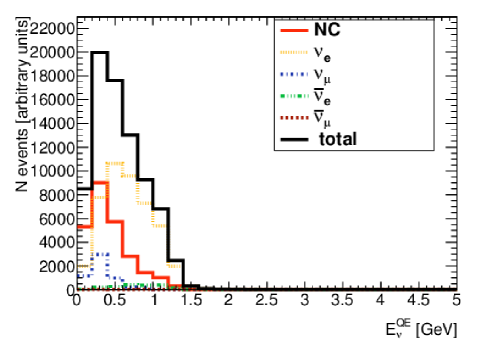
(a) $\mathrm{1R}e$ $\nu$-mode

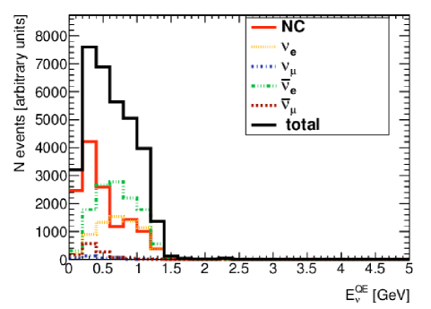
(b) $\mathrm{1R}e$ $\overline{\nu}$-mode

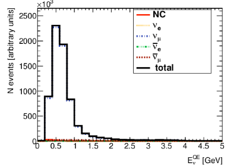
(c) $\mathrm{1R}\mu$ $\nu$-mode

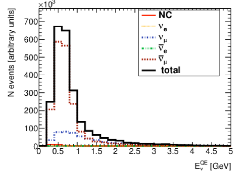
(d) $\mathrm{1R}\mu$ $\overline{\nu}$-mode

Figure 15: E${}_{\nu}^{\text{QE}}$ distribution of the TITUS $\mathrm{1R}e$ (upper plots) and $\mathrm{1R}\mu$ (lower plots) samples for the neutrino (left plots) and antineutrino (right plots) modes, respectively.

7.3 Neutron selection

True CCQE reactions yield final-state neutrons for antineutrinos ($\overline{\nu}p\rightarrow l^{+}n$) but not for neutrinos ($\nu n\rightarrow l^{-}p$). Although this can be modified by final-state interactions, neutron tagging should still permit the selection of signal-enhanced samples by imposing a neutron requirement or veto for the $\overline{\nu}$ or $\nu$ mode respectively. For the purposes of this discussion, the “signal” is defined as a true $\nu$CCQE interaction during $\nu$-mode running, and as a true $\overline{\nu}$CCQE interaction in $\overline{\nu}$ mode.

The true neutron kinetic energy after FSI is shown in Figure 17, its path length in Figure 17 and the reconstructed energy $E^{QE}_{\nu}$ and its resolution are shown in Figures 18 and 19 for the $\overline{\nu}$-mode and $\nu$-mode running respectively. The breakdown of the selected sample by event topology and the signal-to-background ratio are given in Table 12.

Imposing a neutron veto in $\nu$-mode running improves the sample purity from $74\,\%$ to $83\,\%$ and the signal-to-background ratio from 2.9 to 4.9. The increased purity also improves the energy resolution, as shown in Figure 19, by reducing non-CCQE backgrounds which are incorrectly reconstructed. Conversely, requiring a neutron in $\overline{\nu}$-mode halves the wrong-sign CCQE background from 13% to 7%, increasing the signal purity from 61% to 73% and almost doubling the signal-to-background ratio. In addition, reversing the neutron selection/veto provides a background-enhanced sample which can be used for data-driven background studies.”

Figure 16: The true kinetic energy of neutrons after final state interactions within the nucleus but before secondary interactions within the water volume.

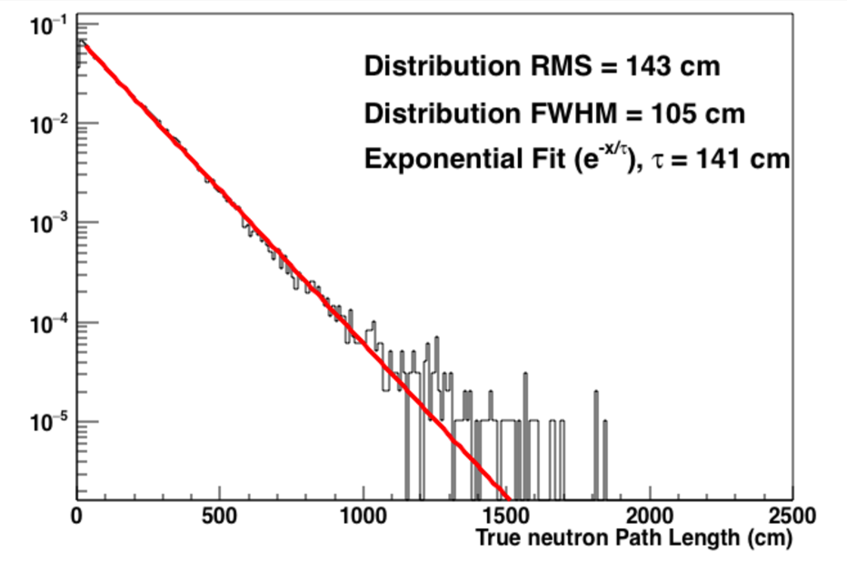
Figure 17: The path length of neutrons emitted from events more than 2 m from the walls of the TITUS detector before capture. This figure was obtained from simulations of $\nu$-mode beam events in TITUS.

Table 12: Neutron (N) selection with gadolinium capture and the 1R$\mu$ event selection.

		Fraction			S/B
Beam Mode	Event Topology	Any N	N$=$1	N=0	Any N	N$=$1	N=0
$\nu$-mode	$\nu$ CCQE	0.74	0.66	0.83	2.87	1.93	4.90
	$\nu$ CC-other	0.23	0.30	0.16	0.30	0.43	0.19
	$\overline{\nu}$ CCQE	0.02	0.03	0.01	0.02	0.03	0.01
	$\overline{\nu}$ CC-other	0.01	0.01	0.00	0.01	0.01	0.00
	NC	0.01	0.01	0.00	0.01	0.01	0.00
$\overline{\nu}$-mode	$\nu$ CCQE	0.13	0.07	0.27	0.15	0.07	0.37
	$\nu$ CC-other	0.08	0.06	0.09	0.09	0.06	0.10
	$\overline{\nu}$ CCQE	0.61	0.73	0.59	1.54	2.67	1.42
	$\overline{\nu}$ CC-other	0.17	0.14	0.04	0.20	0.17	0.05
	NC	0.01	0.00	0.01	0.01	0.00	0.01

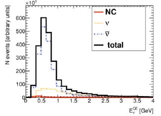
(a) Any $N_{\mathrm{neutrons}}$

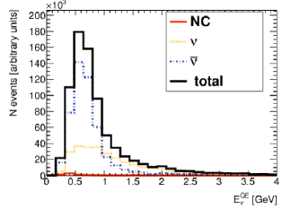
(b) $N_{\mathrm{neutrons}}=0$

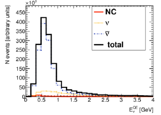
(c) $N_{\mathrm{neutrons}}\geq 1$

Figure 18: The E${}_{\nu}^{QE}$ distributions for the 1R$\mu$ sample during antineutrino mode running for different selections on the number of neutrons, $N_{\text{neutrons}}$: any neutrons, $N_{\text{neutrons}}$ = 0 and $N_{\text{neutrons}}\geq 1$.

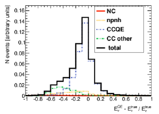
(a) Any $N_{\mathrm{neutrons}}$

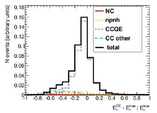
(b) $N_{\mathrm{neutrons}}=0$

(c) $N_{\mathrm{neutrons}}\geq 1$

Figure 19: The E${}_{\nu}^{QE}$ distributions for the 1R$\mu$ sample during neutrino mode running for different selections on the number of neutrons, $N_{\text{neutrons}}$: any neutrons, $N_{\text{neutrons}}$ = 0 and $N_{\text{neutrons}}\geq 1$.

7.4 Systematic Uncertainty on Selected Event Sample

The effects of flux and cross-section systematic uncertainties on the selected samples at TITUS and Hyper-K have been evaluated. The flux systematic uncertainty is based on the error model used by T2K [7]. Assumptions have been made about the ultimate performance of the T2K experiment, including the use of replica target data from the NA61/SHINE experiment. The prior uncertainty is estimated to be around 6%. There is almost 100% correlation between the total fluxes in each running mode between TITUS and Hyper-K detectors, which leads to a significant cancellation of uncertainties. There is a 60% correlation between $\nu$-mode and $\overline{\nu}$-mode running modes, which again will lead to some cancellation of uncertainties.

The interaction uncertainty model is based on the T2K interaction uncertainties used as prior input to T2K oscillation analyses as in Ref. [2]. This model was modified to include an uncertainty of 50% on the normalisation of npnh events and an estimate of the nucleon FSI uncertainties. A 2% uncertainty is set on the $\nu_{e}/\nu_{\mu}$ cross section ratio. This is assumed to be anticorrelated between $\nu$ and $\overline{\nu}$ interactions (the most conservative estimate for the $\delta_{CP}$ measurement).

A rigorous evaluation of the nucleon FSI uncertainties for the NEUT Monte Carlo generator is an ongoing effort within the T2K collaboration and not available at the time of this study. The nucleon FSI errors were evaluated with the GENIE event generator [39], which provides reweighting tools to vary parameters of the FSI model. A GENIE event samples for the TITUS $\nu$-mode and $\overline{\nu}$-mode neutrino fluxes were generated. The nucleon mean free path and probabilities of elastic scattering, multi-nucleon knockout, pion production and charge exchange processes were varied within their default uncertainties as provided by GENIE. The variation in the GENIE neutron multiplicity due to these uncertainties was applied to the NEUT neutron multiplicity. The resulting uncertainty on the neutron multiplicity distribution assumed in this analysis is shown in Figure 20. TITUS itself and other dedicated experiments will provide a direct experimental constraints on the neutron multiplicity for neutrino-Oxygen interactions. The current uncertainties only refer to the NEUT generator as used in this analysis. Differences with other generators may be larger.

Figure 20: The reconstructed neutron multiplicity distribution for $\nu_{\mu}$ and $\overline{\nu}_{\mu}$ events during antineutrino beam mode running. The error bars show the systematic uncertainty on the shape of the reconstructed number of neutrons distribution.

The effect of the systematic uncertainty on the total number of events observed is shown in Table 13. In Hyper-K the event rate in the $\mathrm{1R}e$ sample is used and oscillation is taken into account. The total systematic uncertainty on the absolute event rate, without including a near detector, is $\sim$16%. This is dominated by the large neutrino-nucleus cross section uncertainty. Including the measurements of TITUS the total systematic error is reduced to $\sim$3-4%. The TITUS statistical error is negligible. The statistical error (dominated by the event rate at Hyper-K) is $\sim$2  %.

Table 13: The effect of each systematic uncertainty on the Hyper-K appearance event samples. The size of each systematic is shown both before and after taking into account the TITUS near detector information.

	$\nu$ mode		$\overline{\nu}$ mode
Systematic	No ND	With TITUS	No ND	With TITUS
Interaction Syst.	13.6	1.4	11.5	1.0
Flux Syst.	7.5	0.8	8.0	1.0
Detector + FSI + PN	3.0	2.4	2.1	1.5
Total Syst.	16.1	3.9	14.5	3.5
Statistical	1.8	1.8	1.9	1.9
Stat. + Syst.	16.2	4.3	14.6	4.0

7.5 Sensitivity studies

7.5.1 Fit Method

The selected event samples are binned in 2D where one axis corresponds to the true neutrino energy and the second axis corresponds to the observable bin. The true $E_{\nu}$ bin edges are: (0.2, 0.4, 0.5, 0.6, 0.7, 1.0, 1.5, 2.5, 3.5, 5.0, 7.0, 30.0) GeV. These are chosen to match the input flux error matrix binning. The observable bins are combinations of:

• selected sample (2 options: $\mathrm{1R}e$ or $\mathrm{1R}\mu$);

• detector (2 options: TITUS or Hyper-K);

• beam mode (2 options: $\nu$-mode or $\overline{\nu}$-mode);

• reconstructed neutrino energy (6 options with bin edges: 0.2, 0.4, 0.6, 0.7, 1.0, 1.5, 30.0 GeV)

for a total of 48 bins. Optionally the observable binning could include:

• the number of tagged neutrons, $N$, (either 2 bins for “binary” tagging $N=0$, $N\geq 1$ or 3 bins for “counting” $N=0$, $N=1$, $N\geq 2$),

allowing up to 144 bins when both neutron counting and reconstructed neutrino energy information are used.

To simulate observed event rate vectors in the far detector after oscillation, the following weights are applied:

$$E^{\mathrm{selected}}_{\textrm{with osc.}}(i,{\bm{\theta}})=\sum_{j}^{E_{\nu}^{\mathrm{true}}\textrm{ bins}}{\sum_{k}^{\nu\textrm{ }\mathrm{type}}{\epsilon(i,j,k)\sum_{l}^{\nu\textrm{ }\mathrm{type}}{E(i,j,l)P(\nu_{l}\to\nu_{k}\lvert{\bm{\theta}})}}},$$ (1)

where $i$ corresponds to observable bins, $j$ corresponds to bins in $E_{\nu}^{\mathrm{true}}$, $k$ corresponds to neutrino flavour and $\bm{\theta}$ are the six oscillation parameters. $E(i,j,k)$ is the expected number of events in each bin before any selection is applied. $P(\nu_{l}\to\nu_{k}|{\bm{\theta}})$ is the 3-flavour neutrino oscillation probability calculated with GLoBES [40], [41]. Each bin is multiplied by the selection efficiency, $\epsilon(i,j,k)$, to give the distribution after selection. The observed number of events is calculated by summing over neutrino type and true neutrino energy.

To estimate the systematic uncertainties, Equation 1 is modified with one additional parameter per observable bin, $w_{i}$,

$$E^{\prime}(i,{\bm{\theta}},w_{i})\equiv E^{\mathrm{selected}}_{\textrm{with osc. and syst.}}(i,{\bm{\theta}},w_{i})=w_{i}E^{\mathrm{selected}}_{\textrm{with osc.}}(i,{\bm{\theta}}).$$ (2)

The standard Poisson log-likelihood is defined as

$$-2\ln(\lambda({\bm{\theta}},{\bm{w}}))=2\sum_{i}{E^{\prime}(i,{\bm{\theta}},w_{i})-O(i)+O(i)\ln\frac{O(i)}{E^{\prime}(i,{\bm{\theta}},w_{i})}}.$$ (3)

where $O(i)$ is the observed events in bin $i$. The observed distribution is set to the Asimov dataset [42] (the most likely data with all parameters at their nominal values).

A Bayesian method is used to calculate the measured values of the oscillation parameters given the (fake) observed data. Gaussian constraints are set on the other oscillation parameters based on the current PDG values as shown in Table 14 with $\theta_{23}$=45^∘. The prior on $\delta_{CP}$ is set to be uniform in $\delta_{CP}$ space. A flat prior is also set on $\sin^{2}2\theta_{13}$, as the PDG value is dominated by the reactor constraint, and it is the goal of Hyper-K to measure $\delta_{CP}$ independently of the constraint from the reactor experiments. The prior on the systematic parameters, $w_{i}$, is assumed to be a multivariate Gaussian. A Monte Carlo method was used to vary the underlying systematic parameters in Table 13 and calculate the covariance of the values $E(i,{\bm{\theta}}^{\textrm{nominal}},1)$. This combined likelihood and prior is input into a Markov Chain Monte Carlo tool to estimate the posterior distribution on the oscillation parameters, ${\bm{\theta}}$.

Table 14: The prior uncertainties on the oscillation parameters. They are Gaussian unless otherwise stated.

Parameter	Nominal value and Prior Uncertainty
$\delta_{CP}$	0.0, uniform in $\delta_{CP}$
$\sin^{2}2\theta_{13}$	0.095, uniform in $\sin^{2}2\theta_{13}$
$\sin^{2}2\theta_{23}$	1.00 $\pm$ 0.03 ($\approx$ $\sin^{2}2\theta_{23}>0.95$ at 90% CL)
$\sin^{2}2\theta_{12}$	0.857 $\pm$ 0.034
$\Delta m^{2}_{32}$	(2.32 $\pm$ 0.10) $\times$ 10${}^{\text{-3}}$ eV${}^{\text{2}}$
$\Delta m^{2}_{21}$	(7.5 $\pm$ 0.2) $\times$ 10${}^{\text{-5}}$ eV${}^{\text{2}}$

The results shown are evaluated for a 1:3 POT ratio for $\nu$ and $\overline{\nu}$ running mode. The $\delta_{CP}$ precision is insensitive to the ratio of $\nu-\overline{\nu}$ running over a wide range of running ratios.

7.5.2 Results

Uncertanties on the number of selected events in the far detector:

Table 15 shows the uncertainty on the far detector $\nu_{e}$ sample given constraints from different combinations of near detector and far detector information.

	$\nu$-mode		$\overline{\nu}$-mode
Near Detector	w/o HK 1R$\mu$	with HK 1R$\mu$	w/o HK 1R$\mu$	with HK 1R$\mu$
No near detector	15.3%	6.0%	14.7%	4.7%
ND280	7.9%	5.5%	6.6%	4.1%
TITUS	4.4%	3.8%	3.9%	3.3%

Table 15: The expected uncertainty on the number of selected events in the far detector single ring electron sample. The uncertainty is shown given constraints from the TITUS and ND280 near detectors and the Hyper-K single ring muon sample.

When excluding the far detector $\nu_{\mu}$ sample from the fit, both the TITUS and ND280 near detectors provide a significant reduction in uncertainty in the number of expected events in the far detector electron sample. However, the constraint on the $\nu_{e}$ sample from far detector $\nu_{\mu}$ sample uncertainty is very strong and changes the balance when included in the fit. This is based on the assumptions on the fit made in the subsection 7.5.1. However, the ND280 sample used in this analysis does not not contain a $\nu_{e}$ sample and one should expect better performance from an ND280 sample that includes a direct measurement of the un-oscillated intrinsic $\nu_{e}$ spectrum.

Performance:

Figure 22 shows the expected 90% credible interval on $\delta_{CP}$ and $\sin^{2}{2\theta_{13}}$. The precision on $\delta_{CP}$ assuming $\delta_{CP}=0$ is 0.15 radians (or 8.9$\degree$). With no systematic uncertainties, the statistical precision is $0.08$ (4.6$\degree$). The precision as a function of exposure is shown in Figure 22. The Hyper-K with a ND280 analysis achieves a precision of 0.21 radians (12.4$\degree$). Inclusion of the TITUS near detector gives an improvement of $28\%$ compared to Hyper-K plus ND280. Further improvements may be achieved by fitting the ND280 and TITUS data samples simultaneously.

Figure 21: $\delta_{CP}$-sin${}^{2}{2\theta_{13}}$ 90% contour comparing the nominal TITUS+Hyper-K with ND280+HK and Hyper-K only.

Figure 22: $\delta_{CP}$ performance as a function of POT exposure for different configurations. HK$+$TITUS with Gd means both detectors are Gd-doped.

In addition, there is a significant improvement when including neutron tagging information. A $\delta_{CP}$ precision of 0.14 radians (7.8$\degree$) is achieved when including whether a neutron was tagged or not in an event. Inclusion of gadolinium in both the near and far detector gives a 11% improvement in the performance of the experiment. Adding the ability to count the multiplicity of neutrons (the “counting” option) does not give any significant increase in performance over “binary” neutron tagging, based on the current resolutions.

In summary, the addition of the TITUS Water Cherenkov near detector provides significant improvement in the $\delta_{CP}$ precision and therefore the discovery reach of the Hyper-K experiment. Using a systematic error model based on the experience with T2K, TITUS can significantly reduce the systematic uncertainties on the $\delta_{CP}$ measurement. The addition of Gd to both near and far detectors allows the selection of higher purity samples, the use of which improves the $\delta_{CP}$ precision by a further 11%.

8 Full reconstruction sensitivity studies

The simulation and reconstruction software for TITUS is based on the WChSandBox simulation package [31] developed by the ANNIE collaboration and adapted to the TITUS configuration, together with a global reconstruction package developed for TITUS. Both packages are described in the following sections. A selection is devised for the oscillation analysis and, using the reconstructed data, the CP sensitivity results are obtained using the VaLOR fitting method [43]. Simulation and reconstruction of the MRD are in progress as discussed in Sec. 8.2, and will be added in the future. The current results are based on the WC tank only.

8.1 WC simulation

The neutrino interactions are simulated using the both the $\nu_{\mu}$- and $\overline{\nu}_{\mu}$-mode beam fluxes for the 2036 m baseline (see section 3). The neutrino interaction generators used in the studies below are NEUT v5.3.3 and GENIE v2.8.0.

Each generator takes a flux histogram and generates a sample according to the event rate for that particular flavour and horn configuration, assuming interactions are only on water, H₂O. Only the ¹⁶O and ¹H are simulated. The presumed percentage of gadolinium in the water is negligible in terms of the overall event rate and so is ignored in our interaction simulation.

The detector simulation is performed with a fast simulation package called WChSandBox (or “SandBox”). The SandBox package is Geant4-based, with a single volume of 99.8% water and 0.2% gadolinium by mass. SandBox reads in the generator output and propagates the primary tracks, simulating secondary interactions as it does so. Some features of SandBox include:

• a track-matching algorithm to associate the multiple Geant outputs that are produced when scattering occurs;

• separate classification of optical photons and “particles” (including high energy gamma rays);

• detailed information pertaining to neutrons, including the number of neutrons produced, number of neutrons captured, the time and position of the captures, the daughter nucleus produced and energy released from a neutron capture.

The SandBox outputs two files, one that formats the generator information into a ROOT file and the other that contains the output of the detector simulation. The simulation output files are quite large, owing to tracking of individual optical photons. To partially mitigate this, optical photons are prescaled by 50% in SandBox. Even so, a typical simulated event is about 10 MB in size.

To complete the water Cherenkov part of the simulation, photosensors are also required. SandBox does not have this capacity enabled; instead, the sensors are added afterward as a “mask” of optical photons that hit the detector walls. This mask includes user-set details of the wavelength-dependent quantum efficiency, as well as the size, shape, and timing resolution of the photosensor being simulated. The photosensors for each detector surface can be set individually, and “hybrid” surfaces, containing more than one type of sensor, are also possible.

Once the photosensor simulation has been applied, new output ROOT files are stored. These files are considerably smaller, as the intermediate information (e.g., individual optical photons in a shower) has been discarded. These ROOT files are then passed to the reconstruction algorithms described in section 8.1.1.

Figure 23 show event displays in the TITUS tank. Note the neutron capture event in the bottom row.

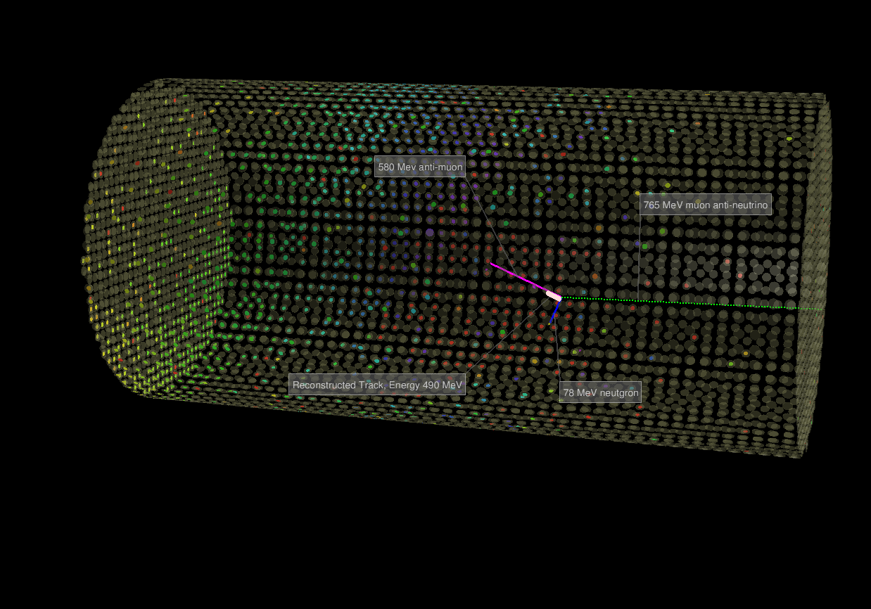
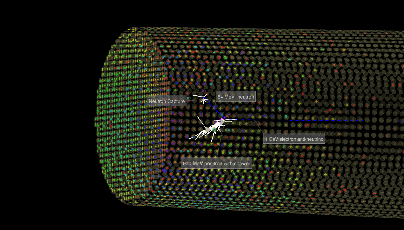
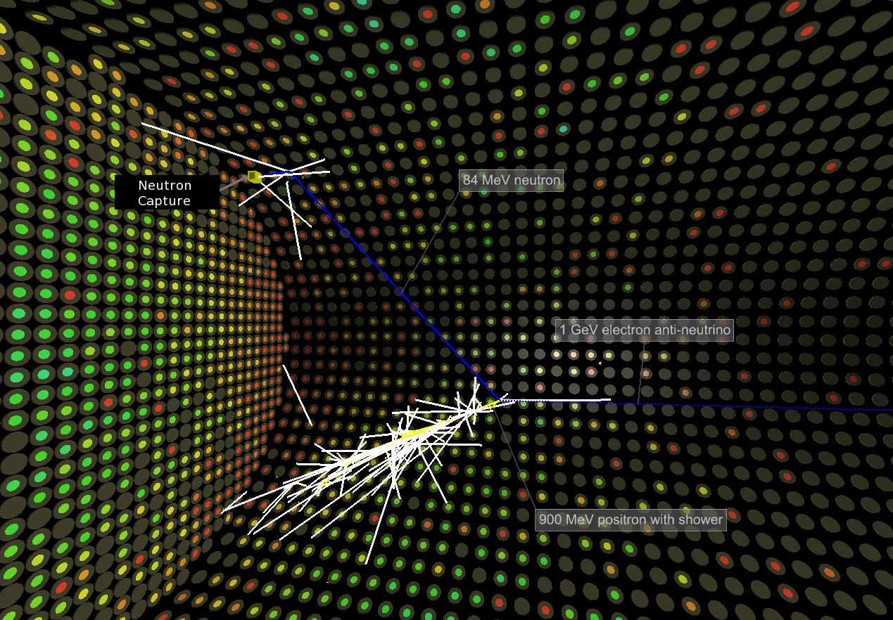
Figure 23: Event displays based on simulated events, shown in 3D, for antineutrino events. Only the WC tank is shown. The first row shows an antineutrino event in two views, the second row shows an antineutrino event in two views with a reconstructed track, and the third row an antineutrino event in two views with neutron capture. White lines are high energy photons, circles represent PMTs and colours indicated charge deposited

The TITUS event display program is based on the “EVE” package in ROOT. It provides a three-dimensional view of events in the TITUS tank as well as a two-dimensional “unrolled” view of the cylindrical tank. The tracks of true particles are shown. The PMTs are represented as a set of circles on the surface of the tank. The total energy falling on each circle is added up and used to colour code the circle when it is displayed.

8.1.1 Event reconstruction

A set of tools has been developed for event reconstruction. All events are first reconstructed using low-energy reconstruction tools. Events that then have an energy above a threshold of 60 MeV, chosen to exclude the majority of secondary sub-events such as Michel electrons and neutron capture signals, are then passed through the high energy reconstruction chain.

The low-energy vertex reconstruction is similar to the “Quad Fitter” method used in SNO and described in section 5.3.2 of Ref. [44]. Combinations of four PMT hits are used to obtain a solution for the position, direction, and time of origin of an interaction. The energy of the event can be approximated from the number of hits recorded by the detector, since they are related linearly.

While low-energy particles can be approximated as a point source, for high-energy particles the non-zero track length must be taken into account, along with the possibility of multiple particles producing Cherenkov rings. The high-energy reconstruction first searches for rings and identifies which observed photoelectrons (PE) belong to each found ring. The timing information of each hit is then used to improve the reconstructed vertex position and direction. Both the muon and electron hypotheses are considered using a look-up-based method to determine the energy and a likelihood-based method of particle identification (PID) to determine whether the ring is electron-like or muon-like.

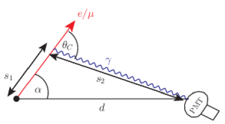
Figure 24: The Hough transform and track fit use time-of-flight information based on the distance the charged particle travels,$s_{1}$, before emitting a photon at angle $\theta_{C}$, which travels distance $s_{2}$ before arriving at a PMT located distance $d$ from the interaction vertex at an angle $\alpha$ to the lepton track.

A Hough transform, similar to that used in Super-K [45], is employed to search for rings. The algorithm converts hits into Hough space from which the centre of the rings can be determined.

The possible directions of the particle responsible for a given hit are calculated using the timing information of each associated PMT hit. The timing information yields a circle of possible directions for each photoelectron origin and the radius of theses circles is dependant on the angle of the particle’s track and the direction from the interaction vertex and the hit PMT, shown in Figure 24. This angle, $\alpha$, is determined from an expression of the time-of-flight (TOF) $t$, using the distance $d$ between reconstructed interaction vertex and hit PMT, and the Cherenkov angle $\theta_{C}$ (which is approximated by that of a particle travelling at $c$)

$$t=\frac{s_{1}}{c}+\frac{n_{\text{ref}}s_{2}}{c}=\frac{d\sin(\theta_{C}-\alpha)}{c\sin\theta_{C}}+\frac{n_{\text{ref}}d\sin\alpha}{c\sin\theta_{C}},$$ (4)

where $n_{\text{ref}}$ is the refractive index. The solution for the angle $\alpha$ is

$$\begin{split}\tan\alpha=\frac{A-B\sqrt{A^{2}-B^{2}+1}}{B^{2}-A^{2}},\\ A=\frac{n_{\text{ref}}-\cos\theta_{C}}{\sin\theta_{C}},\quad B=\frac{ct}{d}.\end{split}$$ (5)

After each ring is found the photoelectrons that are temporally consistent (within twice the timing resolution) with originating from this ring are removed and the algorithm re-run to find additional rings. Any additional ring with less than 9% of the number of hits of the primary ring is discarded. The remainder of the reconstruction is based on the individual rings and the photoelectrons associated to them.

To improve the reconstructed vertex, the PMT hit timing information is used in a fit taking into account the track length of the particle. The algorithm is based on one developed by Super-K [45] using the goodness test value given by

$$G=\sum_{i\in\text{PE}}\exp\left(-\frac{(t^{\prime}_{i}-t_{0})^{2}}{2\sigma^{2}}\right).$$ (6)

where the sum is over all observed photoelectrons, $t^{\prime}_{i}=t_{i}-t_{i}^{\text{exp}}$ is the timing residual determined by the expected total TOF ($t_{i}^{\text{exp}}$) and PMT hit time ($t_{i}$) of the $i$th observed photoelectron, $t_{0}$ is determined by taking the mean value of the $t^{\prime}_{i}$. $\sigma$ is the time spread including PMT transit time spread (TTS) and chromatic dispersions.

Starting from the seed vertex position given by the low-energy reconstruction and the seed direction from the Hough transform and maximising $G$ for the calculated TOF allows the algorithm to estimate the vertex position and direction.

To reconstruct the energy, a lookup table is used based on the total number of photoelectrons observed in the PMTs and the reconstructed distance from the interaction vertex to the wall of the tank. The lookup tables are generated from a Monte-Carlo simulation of CCQE beam events in TITUS for electrons and muons separately.

Particle identification is based on a likelihood method similar to those used in SNO [46] and MiniBoone [47]. The likelihoods are constructed from two separate Monte-Carlo generated probability distributions: the likelihood of observing the number of photoelectrons at each PMT and the likelihood for the time that each photoelecton is observed. These are then used to calculate the expected number of photons received at a given point or PMT, given its distance from the interaction vertex and angle between the particle’s track and the line from the interaction vertex to this point. The reconstruction performs better with relative numbers of photoelectrons at each PMT due to the non-Poissonian nature. The log-likelihood function for the pattern of PMT hits is given by

$$\log L_{\text{pattern}}= \sum_{i\in\text{PMT}}n_{i}\log p_{i}(x,E,l),$$ (7)

$$p_{i}(x,E,l)= \frac{n_{i}^{\text{exp}}(x,E,l)}{\sum_{j}n_{j}^{\text{exp}}(x,E,l)},$$ (8)

where $n_{i}$ is the observed number of photoelectrons at the $i$th PMT, and $p_{i}$ is the probability of an observed photoelectron at the $i$th PMT and the lookup value $n_{i}^{\text{exp}}(x,E,l)$ is the expected number of photoelectrons observed at a PMT coming from a lepton of type $l$ with track starting at point $x$ with energy $E$.

The likelihood for the arrival time for a photoelectron at a PMT are calculated using similar lookup tables.The log-likelihood function for the timing of PMT hits is given by

$$\log L_{\text{time}}=-\sum_{i\in\text{PE}}\frac{(t_{i}-t_{0}-t_{i}^{\text{exp}})^{2}}{2\sigma^{2}},$$ (9)

where $t_{i}$ is the arrival time of the $i$th photoelectron, $t_{0}$ is the reconstructed interaction time and $t_{i}^{\text{exp}}$ is the expected arrival time.

The total log-likelihood $\log L=\log L_{\text{pattern}}+\log L_{\text{time}}$ is maximised, allowing the reconstructed interaction, vertex position, time and direction to vary, for both electron and muon hypotheses. The difference between the log-likelihood value for the electron hypothesis and that of the muon hypothesis is used to discriminate between particle types. The resolutions obtained for the vertex, direction and energy reconstruction as well as the particle identification are shown in Figure 25, for muons and electrons generated with uniformly distributed random positions within the TITUS tank.

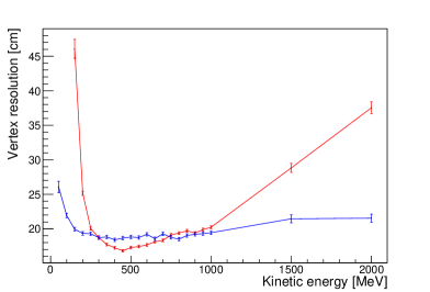
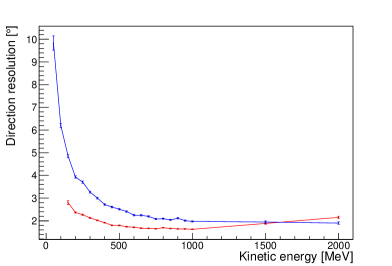
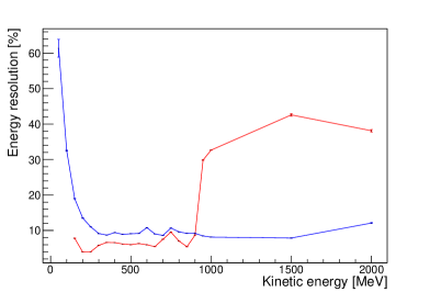
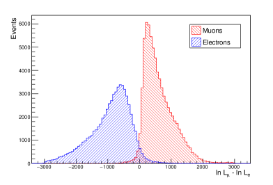
Figure 25: Resolutions of the reconstructed vertex position (top, left), lepton track direction (top, right) and kinetic energy (bottom, left) for muons (red) and electrons (blue) generated at kinetic energies of 50 MeV to 2 GeV for electrons and 150 MeV to 2 GeV for muons. Particle identification for muon and electrons simulated in TITUS (bottom, right).

At low energies, the reconstruction performs poorly due to the smaller number of Cherenkov photons produced. For muons, the vertex reconstruction becomes poor below around 200 MeV, and the direction and energy reconstruction fails at around 100 MeV. Above 200 MeV, the direction resolution is reasonable to high energies above 2 GeV, but the vertex resolution starts to become worse and energy reconstruction fails above around 1 GeV. This is due to the longer range of higher energy muons resulting in their exiting the tank before depositing the majority of their energy. For those muons which range out of the tank into the MRD it will be possible to improve the reconstruction. For electrons, the resolutions are generally worse, but are stable for a wider range of energies; at low energies, the direction and energy resolutions start to become significantly poorer at around 100 MeV, while all parts of the reconstruction remain reasonable beyond 2 GeV.

8.2 MRD simulation

A full simulation and reconstruction software infrastructure is being developed in concert with work on the Baby-MIND detector [19], a magnetised MRD with the same design as the TITUS MRD, but a smaller transverse footprint.

The MRD detector, formed from magnetised iron plates interleaved with scintillator, with air gaps which improve the charge reconstruction efficiency of low-energy muons, has been simulated in Geant4. Track reconstruction by a Kalman Filter [49] confirms the design efficiencies reported earlier in section 6.2. A dedicated algorithm for the analysis of tracks which traverse a small number of iron planes has been added to the TITUS software framework to optimise the charge reconstruction efficiency at low muon momenta. Although it is not used in the current work, it is planned to be used in future improvements of the analysis.

8.3 Full reconstruction selection

For the current studies, samples have been produced for single muon-like ring (1R$\mu$) and single electron-like ring (1R$e$) events. A number of cuts are made which have been optimised based on the current performance of the reconstruction. For the 1R$\mu$ selection, a single ring is required which is identified as muon-like, with a reconstructed neutrino kinetic energy between 0 and 1.25 GeV. A slightly expanded fiducial volume is used with respect to that used in section 7.1, with cuts applied to the reconstructed vertex requiring the vertex to be located at least 2 m away from the tank wall, and at least 2 m to the wall in the reconstructed lepton track direction. For the 1R$e$ selection, a single ring is required identified as electron-like, with a reconstructed kinetic energy between 0 and 2.5 GeV, and a reconstructed vertex $>2$ m from the tank wall and $>2$ m to the wall in the reconstructed track direction. Furthermore, for the electron selection there is a requirement that no decay electrons are identified, whereas in the muon sample up to one decay electron is permitted. Decay electrons are identified as sub-events following the single ring candidate within the time interval 135–8000 ns and with an energy $\geq$15 MeV.

With these selections, a 90% $\nu_{\mu}$CC0$\pi$ purity and 62% efficiency within the selection fiducial volume (18% efficiency overall) are achieved for the $\nu$-mode 1R$\mu$ sample. A 12.1% pure $\nu_{e}$CC0$\pi$ sample with 34% efficiency within the selection fiducial volume (11.4% efficiency overall) is achieved for the $\nu$-mode 1R$e$ sample. The large contamination of the 1 ring electron sample is due in part to $\nu_{\mu}$NC$\pi^{0}$ events where the secondary ring associated with the $\pi^{0}$ is not positively identified, and part due to unidentified secondary pions. More sophisticated algorithms, e.g. fiTQun [2, 47] used for T2K oscillation analyses since Ref. [48], have been shown to achieve significantly better $\pi^{0}$ rejection, reducing the remaining $\pi^{0}$ contribution by a factor of 9 in the Super-K detector.

$\nu$-mode
Sample	Purity	FV efficiency	Total Efficiency
1R$\mu$	90 .0	61.9	18.1
1R$\mu$ no n followers	95.0	42.2	12.3
1Re	12.1	33.6	11.4
1Re NC$\pi^{0}$ reduction	32.6	33.6	11.4
1Re no n followers	47.0	24.2	8.2
NC$\pi^{0}$	44.0	87.5	29.0

Table 16: Purity and efficiency for the different CC0$\pi$ event samples considered from the full reconstruction chain for the $\nu$-mode. For the NC$\pi^{0}$ the purity and efficiency refer to an NC$\pi^{0}$ sample.

$\nu$-mode
Sample	Purity	FV efficiency	Total Efficiency
1R$\mu$	73.1	54.9	16.9
1R$\mu$ no n followers	46.9	7.0	2.2
1R$\mu$ n followers	79.6	47.9	14.8
1Re	7.0	29.8	10.4
1Re NC$\pi^{0}$ reduction	19.8	29.8	10.4
1Re no n followers	6.9	3.4	1.19
1Re n followers	26.2	26.4	9.2

Table 17: Purity and efficiency for the different CC0$\pi$ event samples considered from the full reconstruction chain for the $\overline{\nu}$-mode.

Applying this reduction to events with a $\pi^{0}$ produced improves the 1 ring electron CC0$\pi$ sample purity to 33% but further improvements with more sophisticated ring-finding algorithms can be expected for the $\nu$-mode 1R$e$ TITUS selection in the future. The CC0$\pi$ purity of the single ring samples is further increased, with an accompanying  30-40% drop in efficiency, if a neutron veto is imposed, which gives CC0$\pi$ electron purity of 47% and CC0$\pi$ muon purity of 95%. The neutron reconstruction efficiency, for all neutron captures, is found to be 86% in the selected fiducial volume, with around 90% of captures on Gd. The efficiency for reconstructing Gd neutron captures is 95%.

A summary of the selection efficiencies and purities for the $\nu$-mode is given in Table 16 and Table 17 presents the efficiencies and purities for the $\overline{\nu}$-mode, where antineutrino CC events are expected to be accompanied by a final state neutron. A summary of the mean resolutions for the correctly identified events over the selected position and energy range is given in Table 18. These are fairly similar to the values assumed by Super-K, used in the basic sensitivity studies, presented in Table 11.

	1R$\mu$	1R$e$
Interaction vertex position [cm]	17	17
Outgoing lepton track direction [degrees]	1.9	2.6
Outgoing lepton kinetic energy [MeV]	59	186
Outgoing lepton kinetic energy [%]	13	21

Table 18: Resolutions for $\nu_{\mu}$CC0$\pi$ events in the single muon-like ring (1R$\mu$) sample and for $\nu_{e}$CC0$\pi$ events in the single electron-like ring (1R$e$) sample for a $\nu$-mode beam.

8.4 Sensitivity studies with full reconstruction events

Sensitivity studies produced using results from the full TITUS reconstruction package detailed in the previous sections are presented in the following sections. The Hyper-K detector is simulated using the Super-K Monte-Carlo 14a with exposure and detector errors scaled appropriately. This study aims to be as close as possible to a full Hyper-K oscillation analysis using currently available inputs and tools.

The study is performed using the VaLOR analysis framework which is used for official T2K analyses [43]. Both the near detector, ND, and the far detector, FD, samples are fitted simultaneously by minimising the global Poisson log likelihood constructed from the expected ($n^{\textrm{exp}}_{ij}$) and observed ($n^{\textrm{obs}}_{ij}$) number of events in each reconstructed energy bin defined in Equation 10.

$$-2\ln(\mathcal{L})=\sum\limits_{i}^{Samples}\sum\limits_{j}^{Bins}2\cdot(n^{exp}_{ij}-n^{obs}_{ij}+n^{obs}_{ij}\cdot\ln(\frac{n^{obs}_{ij}}{n^{exp}_{ij}}))+\mathbb{(f-f_{0})^{T}C^{-1}(f-f_{0})}.$$ (10)

With the predicted number of events in each $j^{th}$ reconstructed energy bin is given by

$$n^{exp}_{ij}=\sum\limits_{m}^{modes}\sum\limits_{t}^{EtrueBins}\sum\limits_{r^{\prime}}^{ErecoBins}\textbf{P}_{i;m;t}\cdot\textbf{T}_{i;j;r^{\prime};\mathbb{f}}\cdot\textbf{S}_{i;m;t;r^{\prime};\mathbb{f}}\cdot N^{MC}_{i;m;r^{\prime};t}.$$ (11)

where $N^{MC}_{i;m;r^{\prime};t}$ denotes the number of events in the input MC template for sample $i$ in the reconstructed energy bin $r^{\prime}$, true energy bin $t$ and of interaction mode $m$. T and S are the systematic parameter weights applied to re-weight the MC for any given set of systematic parameters f detailed in Section 8.5 and P is the oscillation probability applied to true energy bins. The oscillation probability is calculated in a three flavour framework including matter effects in constant density matter. The second term in Equation 11 is a penalty with C, the error matrix, used to incorporate prior constraints on systematic errors in the fit detailed below. Each sample consists of 9 interaction modes (CCQE (charged current quasi-elastic), CCnpnh (charged current with n-particle n-hole interactions), CC1$\pi^{\pm}$ (charged current one charged pion), CCcoh (charged current coherent), CCoth (any other charged current interaction), NC1$\pi^{\pm}$ (neutral current with a charged pion), NC1$\pi^{0}$ (neutral current with a neutral pion), NCcoh (neutral current coherent)) and 8 neutrino types (beam $\nu_{e,\mu}$(bar) and oscillated $\nu_{e,\mu}$(bar)). The studies presented here are performed fitting 4 Hyper-K samples, FHC$1R\mu$, FHC$1Re$, RHC$1R\mu$, RHC$1Re$ currently available from the Super-K MC. For TITUS we include neutron information from Gd doping, using binary tagged samples where each sample is separated into events with $>$0 neutrons and 0 neutrons for a total of 8 samples.

The following binning is used for the MC templates used in the analysis:

• Hyper-K $e$-like : 25 reconstructed energy and 84 true energy bins;

• Hyper-K $\mu$-like : 73 reconstructed energy and 84 true energy bins;

• TITUS $e$-like : 6 reconstructed energy and 13 true energy bins.

• TITUS $\mu$-like : 26 reconstructed energy and 13 true energy bins;

All sensitivity studies shown in this section are performed using an Asimov dataset [42], where the nominal MC is taken to represent the data. The Asimov dataset was chosen because it represents nature, to the best of our knowledge, and is free from any statistical or systematic fluctuations.

Significance and confidence regions are constructed with the constant $\Delta\chi^{2}$ method, with nuisance parameters profiled out. Minimisation is performed with Minuit, using the MIGRAD method. Due to a possible degeneracy in the oscillation space; fits in the parameters $\sin^{2}(\theta_{23})$ and $\delta_{CP}$ are performed multiple times. After the initial fit a subsequent fit is performed seeded at the mirror point, in $\sin^{2}(\theta_{23})$ and $\delta_{CP}$, of the best fit point from the initial fit to ensure the global minimum is found.

The studies presented here were performed for the Hyper-K baseline design assuming a running ratio of 1:3 neutrino:antineutrino mode with a nominal exposure of 1.3 MW$\times$10 y assuming 320 kA horn current. Based on high intensity studies of the current accelerator performance, it is expected that 1.3 MW beam power can be achieved after these upgrades [50] [51].

8.5 Treatment of systematic uncertainty

The analysis considers 189 sources of systematic error from the Hyper-K detector response uncertainty, TITUS detector response uncertainty, flux prediction, and cross section model.

8.5.1 Detector, pion FSI, SI and PN

Detector, PFSI (Pion Final state interaction), SI (Secondary interaction) and PN (Photo nuclear) uncertainties are found using the MC predictions obtained by varying the underlying model parameters based on prior uncertainty from external constraints. A covariance matrix, binned in reconstructed energy bins for the interaction modes of interest, is then produced from the variance in the MC prediction. This allows us to use a detector+PFSI+SI+PN matrix produced by the linear sum of the 4 matrices. Finally, there is also an additional detection energy scale uncertainty on all events.

There are a total of 37 Hyper-K Detector+PFSI+SI+PN parameters which affect reconstructed energy bins, 6 $\mu$-like and 12 $e$-like for neutrino mode samples, as in Ref. [2], and the same antineutrino mode samples. The extra parameter is the energy scale which is used for both modes. Correlations are included between the neutrino and antineutrino mode uncertainties. The detector error matrix is scaled down by a factor of $\sqrt{20}$ to account for the additional constraint from larger statistics from the control samples in the Hyper-K era.

There are a total of 31 TITUS parameters which affect reconstructed energy bins, 15 for neutrino mode and 15 for antineutrino mode, as for Hyper-K with uncertainty on appearance events removed. Again, the last systematic parameter is the energy scale parameter. The detector error matrix is taken unscaled from Ref. [2]. Detector, PFSI, SI and PN uncertainties are treated as fully correlated between the neutron tagged and neutron untagged samples.

The PFSI uncertainties are included as described above and correlations included between all Hyper-K and TITUS samples. SI and PN uncertainties were calculated using only the SK MC and then applied to both TITUS and Hyper-K samples with a 90% correlation included between the two.

8.5.2 Flux

A total of 100 parameters to account for flux uncertainties are applied as normalisations on the true energy bins, 25 for each detector and running mode combination. An error matrix for the flux parameters is used assuming full replica target data from NA61/SHINE which is expected during Hyper-K operation. As a result the pre-fit uncertainty on the flux is greatly reduced compared to what is currently used in T2K oscillation analyses [2].

8.5.3 Cross section

A total 15 cross section model parameter uncertainties applied and implemented using response functions, as in the 2015 T2K oscillation analyses [2]. These include the CCQE axial mass (MaQE 6%), Fermi momentum (7%), binding energy (33%), nucleon to $\Delta$ axial form factor ($C^{A}_{5}$ 12%), resonance production axial mass scaling factor (MaRes 16%), scale of isospin $\frac{1}{2}$ non-resonant background (15%), CCoth shape (40%), npnh normalisation (102%), npnh$\bar{\nu}$ normalisation (102%), CCcoh normalisation (100%), NCcoh normalisation (30%), NCoth normalisation (30%), NC 1$\gamma$ normalisation (100%), CC $\nu_{e}$ normalisation (2%) and CC $\bar{\nu}_{e}$ normalisation (2%)

8.5.4 Nucleon FSI

Nucleon FSI uncertainties are included based on studies performed with the GENIE event generator as described in section 7.1. The result is a set of 6 parameters which parameterise the uncertainty due to nucleon FSI in the studies.

Parameter(s)	Value
$\sin^{2}(\theta_{23})$	0.528
$\sin^{2}(\theta_{13})$	0.0217
$\sin^{2}(2\theta_{12})$	0.846
$|\Delta m^{2}_{32}|$ (NH) / $|\Delta m^{2}_{31}|$ (IH)	$2.509\times 10^{-3}~{}\mbox{eV}^{2}/\mbox{c}^{4}$
$\Delta m^{2}_{21}$	$7.53\times 10^{-5}~{}\mbox{eV}^{2}/\mbox{c}^{4}$
$\delta_{CP}$	$-1.601$
Mass Hierarchy	Normal

Table 19: Values of oscillation parameters used to compute the event rates, systematic effects and sensitivity studies. Each set of oscillation parameters correspond to a different Asimov data set, which is the MC expected distribution in a certain oscillation hypothesis.

8.6 Predicted Hyper-K spectra

The numbers of predicted events rates at Hyper-K are shown in Table 20, Table 21 and Figure 26 according to our tank and beam assumptions, where FHC corresponds to the $\nu$-mode, and RHC corresponds to the $\overline{\nu}$-mode. Notable features which are important for the measurement of $\delta_{CP}$ and $\sin^{2}(\theta_{23})$ include the wrong sign background component of the RHC spectra and the intrinsic beam $\nu_{e}$ component. The TITUS spectra are in Figure 27 and Figure 28 for no neutron tagged and neutron tagged samples, respectively.

	$\nu_{\mu}$ CC	$\bar{\nu}_{\mu}$ CC	$\nu_{e}+\bar{\nu}_{e}$ CC	NC	$\nu_{\mu}\rightarrow\nu_{e}$ CC	$\bar{\nu}_{\mu}\rightarrow\bar{\nu}_{e}$ CC	Total
$\nu$ mode	10	0	383	204	2622	17	3236
$\bar{\nu}$ mode	4	3	479	266	304	1076	2132

Table 20: 1$R_{e}$ event rate breakdown.

	$\nu_{\mu}$ CC	$\bar{\nu}_{\mu}$ CC	$\nu_{e}+\bar{\nu}_{e}$ CC	NC	$\nu_{\mu}\rightarrow\nu_{e}$ CC	$\bar{\nu}_{\mu}\rightarrow\bar{\nu}_{e}$ CC	Total
$\nu$ mode	12315	899	9	1122	44	0	14389
$\bar{\nu}$ mode	7139	12425	10	1321	6	14	20915

Table 21: 1$R\mu$ event rate breakdown.

(a) FHC$1Re$

(b) FHC$1R\mu$

(c) RHC$1Re$

(d) RHC$1R\mu$

Figure 26: Predicted Hyper-K spectra for the oscillation parameters in Table 19.

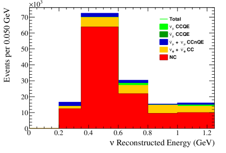
(a) FHC$1Re$

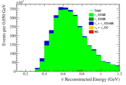
(b) FHC$1R\mu$

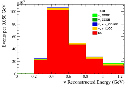
(c) RHC$1Re$

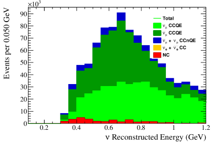
(d) RHC$1R\mu$

Figure 27: Predicted no neutron tagged TITUS spectra.

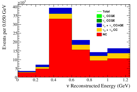
(a) FHC$1Re$

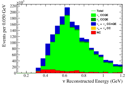
(b) FHC$1R\mu$

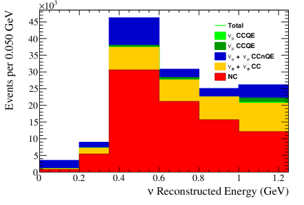
(c) RHC$1Re$

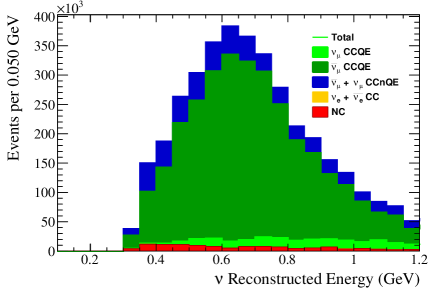
(d) RHC$1R\mu$

Figure 28: Predicted neutron tagged TITUS spectra.

8.7 Systematic variations

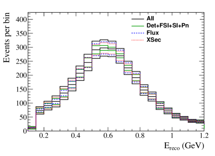
(a) FHC$1Re$

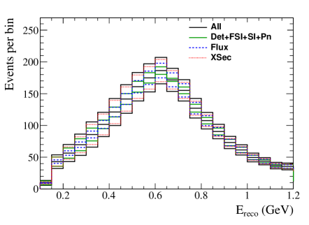
(b) RHC$1Re$

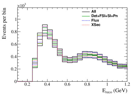
(c) FHC$1R\mu$

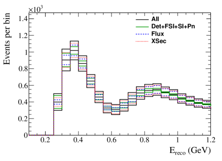
(d) RHC$1R\mu$

(e) Ratio FHC$1Re$/RHC$1Re$

Figure 29: Systematic variations of Hyper-K energy spectra due to fluctuations of systematic parameters produced by randomising the systematic parameters 5,000 times and calculating the root mean squares of each bin. For oscillation parameters given in Table 19.

Figure 29 shows that the uncertainty on each bin in the Hyper-K samples. We see that the cross section and flux errors are the dominant sources of uncertainty on all samples and the detector+PFSI+SI+PN errors have a limited effect. In total the uncertainty on each bin is approximately 10%. Figure 29e shows the uncertainty on the ratio of events in each neutrino mode $1Re$ and antineutrino mode $1Re$ bin, an important quantity to constrain $\delta_{cp}$, is dominated by flux and cross section uncertainties beyond 0.4 MeV where most events occur. This is important as the flux and cross section parameters are what we expect the TITUS samples to constrain most, although they also have some power to constrain PFSI+SI+PN errors.

(a) FHC$1Re$

(b) RHC$1Re$

(c) FHC$1Re$ fractional change

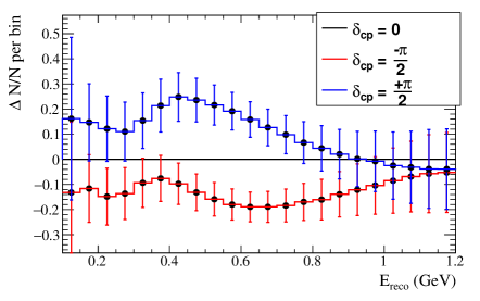
(d) RHC$1Re$ fractional change

(e) FHC$1R\mu$

(f) RHC$1R\mu$

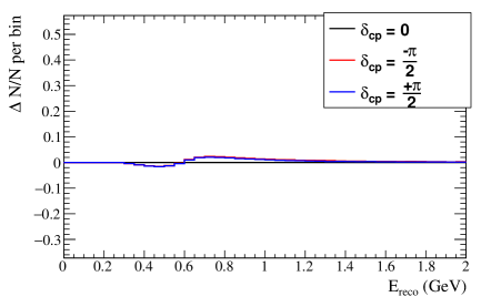
(g) FHC$1R\mu$ fractional change

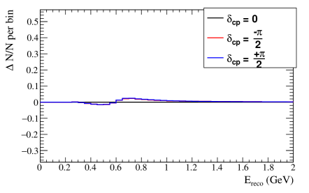
(h) RHC$1R\mu$ fractional change

Figure 30: Effect of $\delta_{CP}$ on Hyper-K spectra.

8.8 $\delta_{CP}$ sensitivity

In Figure 30 we see the effect of $\delta_{CP}$ on the Hyper-K samples. It is clear from this how the effect of $\delta_{CP}$ is confined to the appearance samples and causes a shift in the total event rate by up to 20%. We also see the effect of $\delta_{CP}$ on the shape of the Hyper-K spectra which highlights the importance of the energy resolution for both appearance and disappearance spectra.

8.8.1 CP violation sensitivity

The sensitivity to CP violation is shown in Figure 31. A significant improvement in the sensitivity can be seen with the addition of TITUS samples in the fit. Hyper-K alone, without any near detector constraint, can determine CP violation at the 5$\sigma$ level for 50% of $\delta_{cp}$ space and can provide a 3$\sigma$ measurement for 72%. With the TITUS constraint, Hyper-K will be able to provide a 5$\sigma$ measurement for 62% of $\delta_{cp}$ space, close to the 74% achieved without considering systematic uncertainties.

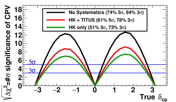
Figure 31: Significance to measure CP violation as a function of $\delta_{CP}$ with Hyper-K only, TITUS (Gd-doped) and Hyper-K (not Gd-doped), and Hyper-K without considering sources of systematic uncertainty. For the studies, the true values of oscillation parameters to generate the data sets were taken from Table 19 but with $\sin^{2}(\theta_{23})=0.5$. The fraction of $\delta_{CP}$ for which CP violation will be measured at 5$\sigma$ and 3$\sigma$ is given in the legend. The sensitivity is for the case of normal hierarchy and assuming it is known.

8.8.2 1D $\delta_{cp}$ fits

The results of 3 Asimov fits to $\delta_{CP}$ are shown in Figure 32 and the constraints achieved given in Table 22. We find that Hyper-K alone provides a weak measurement with the uncertainty in $\delta_{CP}$ up to seven times greater in comparison to the case where no systematic uncertainty is considered. Figure 32 also shows how the likelihood can become asymmetric due to a slight symmetry in the appearance spectra around $\pm\frac{\pi}{2}$, which also act as boundaries, and how the constraint on $\delta_{CP}$ can depend on the true value.

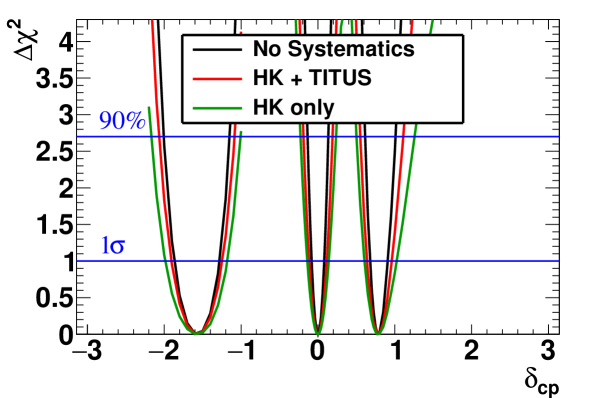
Figure 32: Significance of measuring CP violation as a function of $\delta_{CP}$ with Hyper-K only, TITUS and Hyper-K, and Hyper-K without considering sources of systematic uncertainty for 3 Asimov fits to $\delta_{CP}$. The sensitivity is for the case of normal hierarchy and assuming it is known. The uncertainty on $\delta_{CP}$ is given in Table 22.

	Error (radians/degrees)
True $\delta_{cp}$	No Systematics	Hyper-K only	TITUS + Hyper-K
$0$	0.082 (4.7)	0.139 (8.0)	0.115 (6.6)
$\frac{\pi}{4}$	0.115 (6.6)	0.211 (12.1)	0.161 (9.2)
$-\frac{\pi}{2}$	0.296 (16.9)	0.405 (23.2)	0.332 (19.0)

Table 22: 1 $\sigma$ error (radians/degrees) of $\delta_{cp}$ for each fit shown in Figure 32.

8.9 $23$ sector sensitivity

8.9.1 $\sin^{2}(\theta_{23})\neq 0.5$ sensitivity

The sensitivity to $\sin^{2}(\theta_{23})\neq 0.5$ is shown in Figure 33. The sensitivity increases as true $\sin^{2}(\theta_{23})$ is away from 0.5 however the exclusion is not symmetric around 0.5. Due to the non zero value of $\sin^{2}(\theta_{13})$, the disappearance spectra have a symmetry around $\sin^{2}(\theta_{23})=0.513$, which is the cause of the flat feature in the sensitivity between 0.5 and 0.53. As expected, there is an improvement in the sensitivity to $\sin^{2}(\theta_{23})\neq 0.5$ when TITUS is included in the fit increasing the amount of $\sin^{2}(\theta_{23})$ space by 2%, halfway to the possible 91% in the case of no systematic uncertainty. The improvement is however not as drastic as in the case of the CP violation measurement, as constraints on the cross section model parameters and flux prior to the fit lead to a small uncertainty on the shape of the oscillation dip in the disappearance spectra.

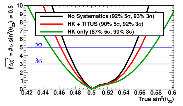
Figure 33: Significance to exclude $\sin^{2}(\theta_{23})=0.5$ as a function of $\sin^{2}(\theta_{23})$ with the combinations of samples and constraints given in the legend and the fraction of $\sin^{2}(\theta_{23})$ Hyper-K will be able to exclude $\sin^{2}(\theta_{23})=0.5$ (at 5$\sigma$ and 3$\sigma$). For the studies, the true values of oscillation parameters to generate the data sets were taken from Table 19. Sensitivity is for the case of normal hierarchy and assuming it is known. Due to a non zero $\sin^{2}(\theta_{13})$, the disappearance spectra have a symmetry around $\sin^{2}(\theta_{23})=0.511$, which is the cause of the flat feature in the sensitivity between 0.5 and 0.511.

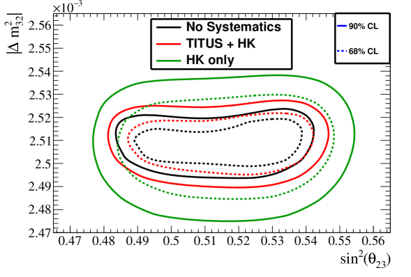
Figure 34: The 68% and 90% confidence level contours for an Asimov fit of $\sin^{2}(\theta_{23})$ and $\Delta m^{2}_{32}$ for the cases of no systematic uncertainty, only HK constraint and both TITUS and HK constraints, are shown. Confidence contours were made with the constant $\Delta\chi^{2}$ method. For the studies, the true values of oscillation parameters to generate the data sets were taken from Table 19. All oscillation and systematic parameters were profiled in the production of the contours except the hierarchy which was fixed to normal.

8.9.2 $\sin^{2}(\theta_{23})$ vs $\Delta m^{2}_{32}$

The sensitivity of an Asimov fit for the parameters $\sin^{2}(\theta_{23})$ vs $\Delta m^{2}_{32}$ is shown in Figure 34. In all fits we see the symmetry around the point of maximal disappearance at $\sin^{2}(\theta_{23})=0.511$ however, as the true value is close to the point of maximal disappearance, there is almost no sensitivity to the octant of $\sin^{2}(\theta_{23})$ in any of the fits and the contours are symmetric. The TITUS samples greatly improve the sensitivity to the 23 sector parameters; note that the 90% CL contour from the TITUS+Hyper-K fit falling within the Hyper-K only 68% CL contour. With the TITUS constraint the expected 90% CL ranges are approximately 0.480 - 0.548 in $\sin^{2}(\theta_{23})$ and 0.00249 - 0.00253 (eV/c²)² in $\Delta m^{2}_{32}$.

A summary of the sensitivities are given in Table 23 and Table 24.

Parameter(s)	3 $\sigma$	5 $\sigma$
TITUS + HK	78%	61%
HK only	73%	51%
No systematics	84%	74%

Table 23: Summary of the percentage of $\delta_{CP}$ space for which there is expected to be a measurement of CP violation at 3 $\sigma$ and 5 $\sigma$ significance.

Parameter(s)	3 $\sigma$	5 $\sigma$
TITUS + HK	92%	90%
HK only	90%	87%
No systematics	93%	92%

Table 24: Summary of the percentage of $\sin^{2}(\theta_{23})$ space for which there is expected to be a measurement which excludes $\sin^{2}(\theta_{23})=0.5$ at 3 $\sigma$ and 5 $\sigma$ significance.

8.10 T2K phase-2 sensitivity

The $\delta_{cp}$ fit and CP violation sensitivity studies were also performed for the T2K phase-2 setup with the addition of a TITUS constraint. In these studies the systematic model was maintained from the Hyper-K fits but exposures of each detector were scaled to the size and beam power $\times$ time. Additionally, the exposure was scaled to account for the expected increase in fiducial volume expected for Super Kamiokande [3]. The sensitivity to CP violation is shown in Figure 35 and the $\delta_{cp}$ sensitivity is shown in Figure 36 and Table 25.

The sensitivity to non maximal mixing is shown in Figure 37.

From these studies we see that TITUS is able to limit the dominant systematics effectively for the case of a $\delta_{cp}$ and CPV measurement as the Super Kamiokande + TITUS combination has very similar sensitivity to the case with no systematic uncertainty. In the case of excluding maximal mixing, TITUS offers some improvement in the sensitivity but could also do better with optimisation.

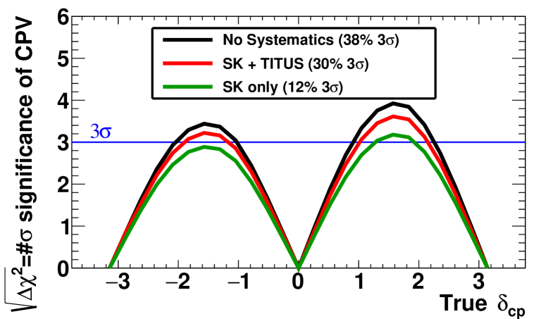
Figure 35: Significance to measure CP violation as a function of $\delta_{cp}$ with T2K phase-2 only, TITUS and T2K phase-2, and T2K phase-2 without considering sources of systematic uncertainty assuming T2K phase-2 statistics. For the studies, the true values of oscillation parameters to generate the data sets were taken from Table 19 but with $\sin^{2}(\theta_{23})=0.5$. The fraction of $\delta_{cp}$ for which CP violation will be measured at 5$\sigma$ and 3$\sigma$ is given in the legend. The sensitivity is for the case of normal hierarchy and assuming it is known.

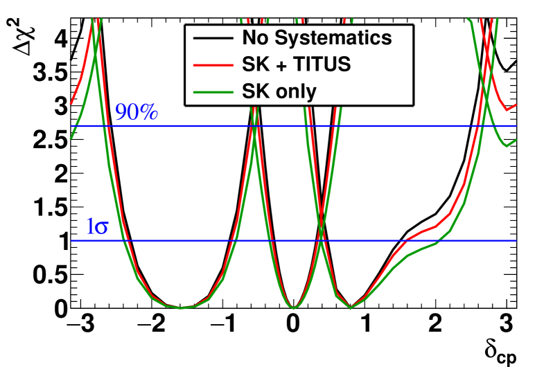
Figure 36: Significance to measure CP violation as a function of $\delta_{cp}$ with T2K phase-2 only, TITUS and T2K phase-2, and T2K phase-2 without considering sources of systematic uncertainty for 3 Asimov fits to $\delta_{cp}$ assuming T2K phase-2 statistics. The sensitivity is for the case of normal hierarchy and assuming it is known. The uncertainty on $\delta_{cp}$ is given in Table 25 and the other oscillation parameters are given in Table 19.

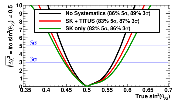
Figure 37: Significance to exclude $\sin^{2}(\theta_{23})=0.5$ as a function of $\sin^{2}(\theta_{23})$ with the combinations of samples and constraints given in the legend and the fraction of $\sin^{2}(\theta_{23})$ Super-K will be able to exclude $\sin^{2}(\theta_{23})=0.5$ (at 5$\sigma$ and 3$\sigma$). For the studies, the true values of oscillation parameters to generate the data sets were taken from Table 19. Sensitivity is for the case of normal hierarchy and assuming it is known. Due to a non zero $\sin^{2}(\theta_{13})$, the disappearance spectra have a symmetry around $\sin^{2}(\theta_{23})=0.511$, which is the cause of the flat feature in the sensitivity between 0.5 and 0.511.

	Error (radians/degrees)
True $\delta_{cp}$	No Systematics	T2K phase-2 only	TITUS + T2K phase-2
$0$	0.296 (17.0)	0.359 (20.6)	0.316 (18.1)
$\frac{\pi}{4}$	0.514 (29.5)	0.839 (48.1)	0.577 (33.1)
$-\frac{\pi}{2}$	0.709 (40.6)	0.790 (45.3)	0.737 (42.2)

Table 25: 1$\sigma$ error (radians/degrees) of $\delta_{CP}$ for each fit for T2K phase-2 shown in Figure 36.

9 Other physics

The physics programme of the TITUS detector goes beyond oscillation analysis. The detector will be able to provide new important measurements on neutrino cross sections; it will have the unique ability to measure the neutron content of the cross sections. It will also be able to address possible precision measurements like the weak mixing angle, the strangeness content of the nucleus and isospin physics. Moreover, the experiment maybe able to generate a supernova alarm and perform interesting physics with the detected events. Finally, it can look at WIMP signatures and non-standard neutrino interactions. In the following sections, a more detailed look at these processes will be given.

9.1 Neutrino cross sections

Cherenkov detectors exhibit excellent kinematic coverage due to their 4$\pi$ angular acceptance [52]. Located near to the beam production point, a sizeable Cherenkov detector will offer significant statistics for cross-section studies. In Table 26 we give estimated statistics for various event samples in a 2 kton water Cherenkov detector, with a 1 m from wall fiducial volume cut, at 2 km (2.5^∘ off-axis) and a 1.3 MW beam, corresponding to a total of 27.05$\times 10^{21}$ POT for 10 years. The event samples for this analysis are defined by topology, i.e. the number of mesons in the final state, such that 1$\pi$ is one charged pion in the final state with no other mesons. We use a similar approach to that adopted for the basic selection in section 7.

Selection	Cuts	Nevents	Selection Characteristics
$\nu_{e}$CC0$\pi$ enhanced	1Re FCFV, 0DE, $E_{vis}>100$ MeV	350k	$\epsilon\approx$ 41%, $P\approx$ 61%
$\nu_{\mu}$CC0$\pi$ enhanced	1R$\mu$, $<2$DE, $p_{\mu}>$200 MeV	25M	$\epsilon\approx$ 58%, $P\approx$ 90%
$\nu_{e}$CC1$\pi$ enhanced	1Re FCFV, 1DE, $E_{vis}>$100 MeV	180k	$\epsilon\approx$ 12%, $P\approx$ 21%
$\nu_{\mu}$CC1$\pi$ enhanced	1R$\mu$, $2$DE, $p_{\mu}>$200 MeV	2.3M	$\epsilon\approx$ 17% , $P\approx$ 90%
NC$\pi^{0}$ enhanced	2Re FCFV, 0DE, $85<m_{\rm invariant}<185$ MeV/c2	1.5M	$\epsilon\approx$ 40%, $P\approx$ 88%

Table 26: Some of the primary cross-section measurements accessible with a 2 kton water Cherenkov detector at 2 km from the beamline. The predicted numbers of events have been evaluated for 27.05$\times 10^{21}$POT. The efficiency, $\epsilon$ is the number of selected events divided by the total number of events for the given topology, the purity $P$ is the number of events of a given topology divided by the total events selected. Key to Cuts: FCFV = fully contained in the fiducial volume of a 2.09 kton inner detector. 1Re/$\mu$ = 1 electron/muon type ring, DE = decay electrons identified, $m_{\rm invariant}$ = reconstructed invariant mass.

Improvements in our understanding of the underlying interaction mechanism are expected in the near future with ongoing T2K analyses and hence these estimates are considered conservative. Expressing cross-sections as a ratio takes advantage of the cancellation of correlated systematic sources, in particular flux uncertainties, to maximise the accuracy of extracted information. These studies indicate that the $\nu_{e}$CC0$\pi$/$\nu_{\mu}$CC0$\pi$ cross section ratio can be measured to 3.2% accuracy, dominated by a 3.1% contribution from cross section uncertainties. The NC$\pi^{0}$/$\nu_{\mu}$CC0$\pi$ cross section ratio can be measured to an accuracy of 14.8% again dominated by cross section uncertainties.

To put these measurement predictions into context, the $\nu_{e}$ cross-section ratio would give significant improvement over existing results: the T2K experiment has published a $\nu_{e}$ charged current cross-section measurement on carbon to 18% precision[53] and compared the interaction rate on water to the predicted rate with 45% precision[54]. TITUS can improve upon these measurements due to the large active water target volume. Furthermore, with further reduction of other cross-section uncertainties from proceeding T2K analyses, the 3.2% accuracy predicted here can be considered a conservative bound. For the NC$\pi^{0}$ ratio, the MiniBooNE experiment have published a measurement of the single $\pi^{0}$ production cross-section on mineral oil with 16% accuracy[55] and the ArgoNeuT collaboration have measured the NC$\pi^{0}$ to CC cross-section ratio on an argon target with 28% precision[56]. The only existing measurement on a water target is from the K2K collaboration, who give a non-differential NC$\pi^{0}$ to total charged current cross section ratio with 11% precision[57], but with a number of model-dependent assumptions that yield significantly lower uncertainties than current thinking on neutrino interaction model uncertainty. Despite the lower beam energy, the larger exposure and target volume should yield nearly 24 times as many selected NC$\pi^{0}$ events in TITUS as K2K.

The selections in Table 26 do not include any neutron tagging information. However, gadolinium doped water Cherenkov detectors, such as TITUS, provide a natural path to future neutrino cross-section measurements with neutron tagging of the final state.

A statistical separation of interaction types based on neutron multiplicity described in section 4 can offer a new way to measure exclusive differential cross-sections by Cherenkov detectors, and could provide the first measurement of a genuine CCQE cross-section by a Cherenkov detector. An example of which would be the $\overline{\nu}_{\mu}$CC0$\pi$ cross section as a function of neutron multiplicity, as seen in Figure 38. It is also expected that the inelastic channels are accompanied by nucleon emissions [13]. Therefore, detailed measurements of neutron multiplicity also opens a way to study inelastic channels, mainly the $\Delta$ resonance.

Figure 38: True flux-integrated cross section as a function of neutron multiplicity for $\nu_{\mu}$ (black) and $\overline{\nu}_{\mu}$ (red) CC0$\pi$ using the NEUT generator. The $\nu$-mode ($\overline{\nu}$-mode) measurement is on the left(right). Statistical and systematic uncertainties have not been considered. The last bin is integrated for all events with neutron captures greater than 1.

Furthermore, TITUS can help to reduce the main background to proton decays in e${}^{+}\pi^{0}$, which comes from atmospheric neutrinos. Neutron tagging is used to reject background events by requiring signal without neutron candidate events in the final state. A measurement of the neutron content in the candidate events will provide an important input to the background determination for proton decays.

9.2 Standard Model measurements

Neutrinos are natural probes of electroweak physics and TITUS can perform several important measurements, a few of which are discussed here. The $4\pi$ angular coverage of the detector will allow to look at both low Q² and Deep Inelastic Scattering (DIS) regions that are needed for the measurements below.

Perhaps the cleanest and most direct method of determining the proton d/u quark ratio at large Bjorken-$x$ is from neutrino and antineutrino DIS on hydrogen. Existing neutrino data on hydrogen have relatively large errors and do not extend beyond $x\,\sim\,$0.5 [58]. A new measurement of neutrino and antineutrino DIS from hydrogen with significantly improved uncertainties would therefore make an important discovery about the d/u behaviour as $x\rightarrow 1$.

TITUS will have neutrino DIS interactions with $x>0.5$, as shown in Figure 39. NEUT was used to simulate $\nu_{\mu}$ interactions using a $\nu$-mode flux of $6.8\times 10^{21}$ POT and $\overline{\nu}_{\mu}$ interactions with the $\overline{\nu}$-mode flux with $20.3\times 10^{21}$ POT. Gaussian systematic errors were thrown with three assumptions for its source: an uncertainty on the cross section of 0.4/E_ν, where the neutrino energy is in GeV; a flat flux uncertainty of 9%, independently thrown for the $\overline{\nu}$-mode and $\nu$-mode configurations; and a flat detector uncertainty of 5%. Uncertainties for $x>0.5$ may be on the order of 20%. A more precise estimation would require a full event reconstruction that would likely need to select multi-ring interactions, more precise treatment of background subtraction mainly of wrong sign neutrino interactions and propagation of hadrons through the nucleus; this would provide new data where there are currently no measurements. Moreover, the above error estimates are conservative, so it is possible to refine them with further study.

Figure 39: Left: Ratio of the $\overline{\nu}_{\mu}$CCDIS to $\nu_{\mu}$CCDIS cross sections as a function of $x$ with statistical and systematic errors given in the text. Right: Measurement of $\sin^{2}\theta_{W}$ as a function of neutrino energy starting from 5 GeV.

In addition, the strange quark content of the proton and its contribution to the proton-spin can be inferred from TITUS data using ratio of NCEL and CCQE cross sections, a procedure which reduces systematic uncertainties. A large observed value of the strange quark contribution to the nucleon spin (axial current), $\Delta$s, would change our understanding of the proton structure. The spin structure of the nucleon also affects the couplings of axions and supersymmetric particles to dark matter.

A measurement of the ratios $\frac{\sigma(\nu_{\mu}p\rightarrow\nu_{\mu}p)}{\sigma(\nu_{\mu}n\rightarrow\mu^{-}p)}$ and $\frac{\sigma(\overline{\nu}_{\mu}p\rightarrow\overline{\nu}_{\mu}p)}{\sigma(\overline{\nu}_{\mu}n\rightarrow\mu^{+}p)}$ to 1% precision would enable the extraction of $\Delta$s with an uncertainty of 0.8% and 0.5% for neutrino and antineutrino ratios, respectively. Current measurements have $\sim$50% [59]. The $\Delta$s analysis requires that TITUS is able to reconstruct protons at just above the proton’s Cherenkov threshold.

A measurement of $\frac{\sigma(\nu_{\mu}p\rightarrow\nu_{\mu}p)}{\sigma(\nu_{\mu}n\rightarrow\nu_{\mu}n)}$ is also possible due to the fact that TITUS is Gd-doped. Assuming $\Delta$s has a value of $-0.1$, an uncertainty of 10% on $\Delta$s requires that the ratio has an uncertainty of 30%. While many systematic uncertainties will cancel in this ratio, the kinematic threshold of the proton, background neutrino interaction subtraction, external neutron backgrounds, and the choice of nuclear model need to be well-understood to attain a measurement of this precision, which would be the first of its kind and would provide the best sensitivity to $\Delta$s if it were non-zero.

Finally, by measuring the ratio of the DIS neutrino NC and CC interactions, TITUS can perform a measurement of the weak mixing angle $\theta_{W}$:

$$R_{\nu}\equiv\frac{\sigma^{\nu}_{NC}-\sigma^{\overline{\nu}}_{NC}}{\sigma^{\nu}_{CC}-\sigma^{\overline{\nu}}_{CC}}\sim\rho^{2}(1-\sin^{2}\theta_{W})$$ (12)

where $\rho$ is from the Paschos-Wolfenstein relations and is taken to be one [60].

A single bin Monte Carlo truth study was performed to get an idea of the precision of such a measurement on neutrino interactions on oxygen using the same generated sample as the $d/u$ measurement discussed above. It was found that an uncertainty of 2.6% on the measurement of $\sin^{2}\theta_{W}$ can be reached. This would be the first measurement of its kind by a water Cherenkov detector and will potentially shed light on the NuTeV anomaly [61].

9.3 Supernova burst

Core collapse supernova explosions are the final evolutionary stage of massive stars, $\gtrsim 8M_{\odot}$. Such explosions release $99\%$ of their energy, estimated to be $\mathcal{O}\left(10^{53}\right)\text{ergs}$, in neutrinos. To date, the only observation made is that of 25 neutrinos from supernova 1987A by the Kamiokande [62], IMB [63] and Baksan [64] detectors. Supernova 1987A occurred in the Large Magellanic Cloud, at a distance of $(50.0\pm 1.1)\,$kpc [65]; if a supernova were to occur within the Milky Way Galaxy, at a likely distance of $\mathcal{O}\left(10\right)\text{kpc}$, then the combination of a 5$\times$ shorter distance and the much larger target masses of current and future detectors leads to an expected event rate several orders of magnitude greater than SN 1987A. These large event rates precede by a few hours the observation of light from supernova explosions, and so can be used as an early warning for astronomers to prepare visible observations through the SuperNova Early Warning System (SNEWS) [66], as well as offering information about the formation of the neutron star and the first few seconds of the subsequent explosion. Additionally, such observations probe interesting neutrino physics such as the neutrino mass ordering and neutrino oscillations.

The TITUS detector, with its reasonably large mass $\left(\sim 2\,\text{kton}\right)$ and potential use of gadolinium doping, should be a useful contributor to the SNEWS network and probe some supernova neutrino interactions in ways unavailable to traditional (not doped) water Cherenkov detectors.

Prediction of the expected neutrino flux from core-collapse supernovae remains a challenging problem in astrophysics. Although the “neutralisation pulse” of $\nu_{e}$ from the formation of the neutron star is easily calculated, it does not dominate the neutrino flux: most neutrinos are produced thermally in the course of the explosion. Modelling the propagation of neutrinos through the explosion is difficult, as the extremely high densities of both electrons and neutrinos produce not only matter-enhanced MSW oscillations, but also collective effects caused by neutrino-neutrino interactions. The latter can be very dramatic, resulting in wholesale exchange of flavours above a particular energy threshold [67]. In addition, 3D simulations of supernova explosions indicate that they are quite asymmetric, and the flux of neutrinos, particularly its detailed time structure, may depend on direction [68].

Initial studies of the expected neutrino interaction rate from a supernova explosion within the TITUS detector have been undertaken using the SNOwGLoBES software package [69], in conjunction with numerical flux predictions developed by Hans-Thomas Janka and colleagues at the Max Planck Institute for Astrophysics, and detailed in the thesis of Lorenz Hüdepohl [70]. The available models include a range of different supernova progenitor masses, two different equations of state for the nuclear environment, and potential inclusion of corrections to the treatment of convection and neutrino-nucleon opacities. In the future the full range of these models will be considered in detail, but for the moment, results are shown for progenitor masses of $11.2M_{\odot}$ and $27.0M_{\odot}$, with the Lattimer and Swesty equation of state [71] with a nuclear compressibility factor $K=220$ MeV and the inclusion of convection and opacity corrections. The predicted integrated fluxes from these two models are shown in Figure 40 for progenitors at a distance of 10 kpc. Note that these results do not currently include the effects of neutrino oscillations.

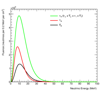
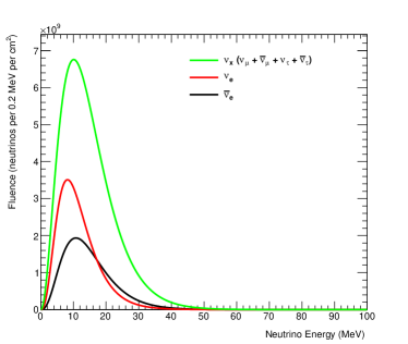
Figure 40: Total predicted neutrino flux for $11.2M_{\odot}$ (left) and $27.0M_{\odot}$ (right) progenitor mass stars at a distance of 10 kpc.

The integrated neutrino flux is then convolved with the relevant neutrino interaction cross-sections for a water target to produce an expected event rate and interaction spectrum within the TITUS detector, as shown in Figure 41 and Table 27.

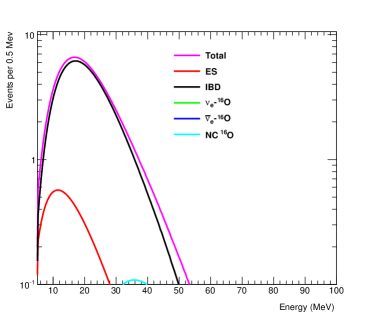
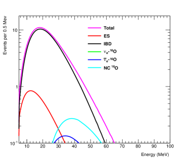
Figure 41: Predicted neutrino interaction spectrum, broken down by interaction type, for $11.2M_{\odot}$ (left) and $27.0M_{\odot}$ (right) progenitor mass stars at a distance of 10 kpc in the TITUS detector. Legend defined in Table 27.

Interaction	Event Rate
Type	$11.2M_{\odot}$	$27.0M_{\odot}$
Elastic Scatter	17.9	29.9
Inverse Beta Decay	233.8	440.2
$\nu_{e}-^{16}$O	0.4	2.1
$\bar{\nu}_{e}-^{16}$O	2.5	7.1
NC 16O	5.3	15.0
Total	260.0	494.2

Table 27: Predicted interaction rates broken down by interaction type, for $11.2M_{\odot}$ and $27.0M_{\odot}$ progenitor mass stars at a distance of 10 kpc in the TITUS detector.

Work is being undertaken to calculate and apply the TITUS detector efficiency and energy reconstruction smearing to the predicted event rates. However, the significant event rate predicted at the TITUS detector should allow it to usefully contribute to the SNEWS network and potentially contribute to interesting physics measurements, particularly through unambiguous identification of inverse beta decay events by neutron capture on gadolinium, offering both background reduction and flavour tagging of $\bar{\nu}_{e}$.

9.4 Dark matter

Astronomical and cosmological observations indicate that a large amount ($\sim 85\%$) of the mass content of the Universe is made of dark matter [72]. Particle candidates under the generic name of weakly interacting massive particles (WIMPs) arise naturally in many theories beyond the Standard Model of particle physics and can be experimentally detected [73]. However, the existing evidence for dark matter provides limited information about its non-gravitational interactions, and many candidates are sufficiently non-relativistic and weakly interacting. This situation may open a more complex hidden sector containing additional light states. [74, 75] Direct detection experiments, such as LUX or XENON100, impose stringent constraints on dark matter with a weak-scale mass, excluding a significant region of the spin-independent cross section versus mass phase space [76, 77]. Along with this, astrophysical and cosmological observations pose constraints on the dark matter relic abundance and self-interaction cross sections, while collider experiments can set bounds on the $U(1)^{\prime}$ dark sector gauge coupling and on the kinetic mixing coefficient [78]. Near detector neutrino beam experiments can probe each region, but it is particularly important in the sub-GeV dark matter mass range, where direct-detection experiments tend to have poor sensitivity.

This “dark force” phenomenology has seen increased interest in recent years, and the presence of light mediators coupled to the Standard Model opens up the possibility to probe it experimentally via the production of dark matter beams directly in fixed target facilities. [79] The scattering of the final “dark” light states in a detector spatially separated from the production point may represent the most efficient search strategy. Moreover, owing to the potentially large production rate, and the existence of large volume near detectors, proton fixed-target facilities focusing on neutrino physics appear to be an optimal means for exploring these scenarios [80].

Light dark matter particle ($\chi$) beams can be generated via two processes: i) direct production, $pp(n)\rightarrow V^{*}\rightarrow\bar{\chi}\chi$, where $V$ is the vector mediator; and ii) indirect production, $pp(n)\rightarrow\phi+...\rightarrow V+...\rightarrow\bar{\chi}\chi$ + …, where $\phi$ is a generic hadron state and $V$ is the vector mediator. Once produced, the dark matter beam propagates along with the neutrinos. The beam, weakly scattering with normal matter, is detectable through neutral current-like elastic scattering processes with electrons or, of most relevance here, with nucleons within the neutrino near detector.

TITUS will be particularly suitable for this measurement. In direct $\chi$-production forward direction emission of dark matter is suppressed, therefore the TITUS off-axis alignment is ideal for capturing a large flux of dark matter, as compared to an on-axis detector. As for signal identification, the dominant background from neutrino elastic scattering can be rejected by exploiting some distinctive characteristics. The dark matter beam has a higher average energy than the neutrino beam ($\sim 12$ GeV for a WIMP of 100 MeV, and $\sim 10$ GeV for a WIMP of 300 MeV, for direct production process and off-axis detector angle of $\theta=2^{\circ}$). This would permit a relatively high cut in momentum transfer in scattering. In addition to that, a much higher cutoff can be observed when the scattering energy approaches the energy of the primary proton beam. In particular, a cusp at the kinematic limits for larger $m_{\chi}$ can be observed, as a result of a degeneracy in the angle between $\chi$ and the beam direction in the lab frame, $\theta$, as a function of its value in the $V$ rest frame. This feature, which can be optimally exploited by off-axis experiments such as TITUS, is an additional tool for signal identification. Another feature lies in the fact that the dark matter beam will be relatively unaffected by turning off or switching the polarity of the magnetic focusing horns, which would alter the neutrino beam significantly. If TITUS is equipped with LAPPDs (section 6.3.3) this will further enhance the time resolution and will provide useful information on the timing structure, as the production mechanism for vector-portal-coupled dark matter is very distinct from the neutrino beam. The expected number of elastic nucleon dark matter scattering events can be expressed as

$$N_{N\chi\rightarrow N\chi}\propto n_{N}\cdot\sum_{prod.}\left(N_{\chi}\cdot\sum_{traj.i}R_{i}\sigma_{N\chi}(E_{i})f(\theta_{i},p_{i})\right),$$ (13)

where $n_{N}$ is the nucleon density in the detector, $N_{\chi}$ is the number of dark matter particle produced (in turn proportional to $N_{\textrm{POT}}$ ), $R_{i}$ is a parameter corresponding to the trajectory of the dark matter path within the detector and $f(\theta_{i},p_{i})$ describes the production via direct and indirect processes, with the former including the $(1-\cos^{2}\theta)$ factor suppressing the $\chi$-production in the forward direction. Based on studies previously performed on the ND280 expected sensitivity [80], TITUS could reach a WIMP-nucleus cross section of the better than $\sim 10^{-40}$ cm² for 300 MeV WIMP from direct production and $5\times 10^{-39}$ cm² for 100 MeV WIMP from indirect production (under the assumptions of the mediator mass, $m_{V}$, between 1 GeV and 400 GeV, and the coupling $\alpha^{\prime}$ to be equal to $\alpha$, so that the coupling with the dark sector is equal to the square of the kinetic mixing coefficient).

10 Conclusions

A description of the TITUS detector, a $\sim$2 ton Gd-doped WC detector with an MRD downstream, as proposed near detector for the Hyper-Kamiokande experiment at about 2 km from the beam target is presented, along with an overview of its physics potential. The physics potential described in this document is only based on the analysis of the WC data and does not include the MRD.
The main goal of the TITUS detector is the improvement of the CP potential of the Hyper-Kamiokande experiment. Two sensitivity studies for CP violation that give consistent results are presented in the text. Using the VaLOR fitting method [43], assuming a 1.3 MW beam, 1:3 POT ratio for $\nu$-mode and $\overline{\nu}$-mode beams, the cross section uncertainties as in the T2K oscillation analysis presented in Ref. [2] Hyper-K and TITUS can determine CP violation at the 5$\sigma$ level for 62% of $\delta_{cp}$ space and can provide a 3$\sigma$ measurement for 79%, close to the 84% achieved without considering systematic uncertainties.
Improvements are also observed in the 23 sector using the TITUS detector.
Finally, the detector is also able to address non-oscillation physics, such as cross section measurements, SM measurements, supernova neutrino and dark matter.

References

- [1] K. Abe et al. [Hyper-Kamiokande Proto- Collaboration], PTEP 2015 (2015) 053C02 doi:10.1093/ptep/ptv061 [arXiv:1502.05199 [hep-ex]].
- [2] K. Abe et al. [T2K Collaboration], Phys. Rev. D 91 (2015) no.7, 072010 doi:10.1103/PhysRevD.91.072010 [arXiv:1502.01550 [hep-ex]].
- [3] S. Cao Neutrino oscillation physics potential of T2K Phase 2 http://www.t2k.org/docs/proc/063/t2k2moriond
- [4] J. F. Beacom and M. R. Vagins, Phys. Rev. Lett. 93 (2004) 171101 doi:10.1103/PhysRevLett.93.171101 [hep-ph/0309300].
- [5] L. Alvarez-Ruso, Y. Hayato and J. Nieves, New J. Phys. 16 (2014) 075015 doi:10.1088/1367-2630/16/7/075015 [arXiv:1403.2673 [hep-ph]].
- [6] K. A. Olive et al. [Particle Data Group Collaboration], Chin. Phys. C 38 (2014) 090001.
- [7] K. Abe et al. [T2K Collaboration], Phys. Rev. D 87 (2013) no.1, 012001 Addendum: [Phys. Rev. D 87 (2013) no.1, 019902] doi:10.1103/PhysRevD.87.012001, 10.1103/PhysRevD.87.019902 [arXiv:1211.0469 [hep-ex]].
- [8] T. Ishida [Hyper-Kamiokande Working Group Collaboration], arXiv:1311.5287 [hep-ex].
- [9] Y. Hayato, Acta Phys. Polon. B 40 (2009) 2477.
- [10] R.E. Meads et al, Proc. Phys. Soc. A 69 (1956) 469.
- [11] J. Cao, Nucl. Instrum. Meth. A 732 (2013) 9. doi:10.1016/j.nima.2013.05.076
- [12] O. Lalakulich, K. Gallmeister and U. Mosel, Phys. Rev. C 86 (2012) no.1, 014614 Erratum: [Phys. Rev. C 90 (2014) no.2, 029902] doi:10.1103/PhysRevC.86.014614, 10.1103/PhysRevC.90.029902 [arXiv:1203.2935 [nucl-th]].
- [13] R. Acciarri et al. [ArgoNeuT Collaboration], Phys. Rev. D 90 (2014) no.1, 012008 doi:10.1103/PhysRevD.90.012008 [arXiv:1405.4261 [nucl-ex]].
- [14] S. Agostinelli et al., Nucl. Instrum. Meth. A 506 (2003) 250.
- [15] C. Galbiati and J. F. Beacom, Phys. Rev. C 72 (2005) 025807 Erratum: [Phys. Rev. C 73 (2006) 049906] doi:10.1103/PhysRevC.73.049906, 10.1103/PhysRevC.72.025807 [hep-ph/0504227].
- [16] S. Aoki et al., Nucl. Instrum. Meth. A 698 (2013) 135 doi:10.1016/j.nima.2012.10.001 [arXiv:1206.3553 [physics.ins-det]].
- [17] O. Mineev et al., JINST 6 (2011) P12004.
- [18] V. Likhacheva et al., Talk given at the NPD RAS Session, 11-14 April 2016, Dubna, Russia.
- [19] R. Asfandiyarov et al., arXiv:1405.6089 [physics.ins-det].
- [20] T. Koga et al., JPS Conf. Proc. 8 (2015) 023003. doi:10.7566/JPSCP.8.023003
- [21] S. Adrian-Martinez et al. [KM3Net Collaboration], arXiv:1601.07459 [astro-ph.IM].
- [22] S. Adrian-Martinez et al. [KM3Net Collaboration], JINST 8 (2013) T03006.
- [23] U.F. Katz et al. [KM3Net Collaboration], Nucl. Instr. and Meth. A, 626-627 (2011) S57-S63.
- [24] P. Amram et al. [ANTARES Collaboration], Nucl. Instrum. Meth. A 484 (2002) 369 doi:10.1016/S0168-9002(01)02026-5 [astro-ph/0112172].
- [25] S. Aiello et al. [NEMO Collaboration], Journal of Instrumentation 8 (2013) P07001.
- [26] O. Kalekin [KM3NeT Collaboration], Nucl. Instrum. Meth. A 623 (2010) 312. doi:10.1016/j.nima.2010.02.232
- [27] G. Barbarino et al., Astropart. Phys. 67 (2015) 18 doi:10.1016/j.astropartphys.2015.01.003 [arXiv:1407.2805 [physics.ins-det]].
- [28] E. Leonora et al. [KM3NeT Collaboration], AIP Conf. Proc. 1630 (2014) 110. doi:10.1063/1.4902784
- [29] B. W. Adams et al. [LAPPD Collaboration], arXiv:1603.01843 [physics.ins-det].
- [30] I. Anghel, arXiv:1310.2654 [physics.ins-det].
- [31] I. Anghel et al. [ANNIE Collaboration], arXiv:1504.01480 [physics.ins-det].
- [32] J. Wang et al., Physics Research A 804 (2015) 84-93 [arXiv:1604.07738 [physics.ins-det]].
- [33] D. Renker and E. Lorenz, JINST 4 (2009) P04004.
- [34] Y. Kudenko [T2K Collaboration], Nucl. Instrum. Meth. A 598 (2009) 289 doi:10.1016/j.nima.2008.08.029 [arXiv:0805.0411 [physics.ins-det]].
- [35] http://www.hamamatsu.com/jp/en/index.html; M. Yokoyama et al., Nucl. Instr. Meth. A610 (2009) 128; A. Vacheret et al., Nucl. Instrum. Meth. A656 (2011) 69.
- [36] F. Hosomi et al., PoS PhotoDet2015 (2016) 046.
- [37] http://www.psi.ch/drs/
- [38] WCSim Collaboration, https://github.com/WCSim/WCSim
- [39] C. Andreopoulos et al., Nucl. Instrum. Meth. A 614 (2010) 87 doi:10.1016/j.nima.2009.12.009 [arXiv:0905.2517 [hep-ph]].
- [40] P. Huber, M. Lindner and W. Winter, Comput. Phys. Commun. 167 (2005) 195 doi:10.1016/j.cpc.2005.01.003 [hep-ph/0407333].
- [41] P. Huber, J. Kopp, M. Lindner, M. Rolinec and W. Winter, Comput. Phys. Commun. 177 (2007) 432 doi:10.1016/j.cpc.2007.05.004 [hep-ph/0701187].
- [42] G. Cowan, K. Cranmer, E. Gross and O. Vitells, Eur. Phys. J. C 71 (2011) 1554 Erratum: [Eur. Phys. J. C 73 (2013) 2501] doi:10.1140/epjc/s10052-011-1554-0, 10.1140/epjc/s10052-013-2501-z [arXiv:1007.1727 [physics.data-an]].
- [43] https://valor.pp.rl.ac.uk/
- [44] S.J. Brice, PhD Thesis: “Monte Carlo and Analysis Techniques for the Sudbury Neutrino Observatory”; http://www.sno.phy.queensu.ca/papers/brice_phd.pdf (1996);
- [45] M. Shiozawa [Super-Kamiokande Collaboration], Nucl. Instrum. Meth. A 433 (1999) 240. doi:10.1016/S0168-9002(99)00359-9
- [46] R.J. Bonventre, PhD Thesis: “Neutron multiplicity in atmospheric neutrino events at the Sudbury Neutrino Observatory” (1996);
- [47] R. B. Patterson, E. M. Laird, Y. Liu, P. D. Meyers, I. Stancu and H. A. Tanaka, Nucl. Instrum. Meth. A 608 (2009) 206 doi:10.1016/j.nima.2009.06.064 [arXiv:0902.2222 [hep-ex]].
- [48] K. Abe et al. [T2K Collaboration], Phys. Rev. Lett. 112 (2014) 061802 doi:10.1103/PhysRevLett.112.061802 [arXiv:1311.4750 [hep-ex]].
- [49] A. Cervera-Villanueva et al., Nucl. Instrum. Meth. A534 (2004) 180-183.
- [50] T. Koseki, “J-PARC Accelerator: achievement and future upgrade”, Talk presented at the Workshop for Neutrino Programs with Facilities in Japan, August 4, 2015 Tokai, Japan.
- [51] T. Kobayashi, “Potential J-PARC beam power improvement and beam delivery before 2026”, Talk presented at the Workshop for Neutrino Programs with Facilities in Japan, August 4, 2015 Tokai.
- [52] A. A. Aguilar-Arevalo et al. [MiniBooNE Collaboration], Phys. Rev. D 81 (2010) 092005 doi:10.1103/PhysRevD.81.092005 [arXiv:1002.2680 [hep-ex]].
- [53] K. Abe et al. [T2K Collaboration], Phys. Rev. Lett. 113 (2014) no.24, 241803 doi:10.1103/PhysRevLett.113.241803 [arXiv:1407.7389 [hep-ex]].
- [54] K. Abe et al. [T2K Collaboration], Phys. Rev. D 91 (2015) 112010 doi:10.1103/PhysRevD.91.112010 [arXiv:1503.08815 [hep-ex]].
- [55] A. A. Aguilar-Arevalo et al. [MiniBooNE Collaboration], Phys. Rev. D 81 (2010) 013005 doi:10.1103/PhysRevD.81.013005 [arXiv:0911.2063 [hep-ex]].
- [56] R. Acciarri et al. [ArgoNeuT Collaboration], [arXiv:1511.00941 [hep-ex]].
- [57] S. Nakayama et al. [K2K Collaboration], Phys. Lett. B 619 (2005) 255 doi:10.1016/j.physletb.2005.05.044 [hep-ex/0408134].
- [58] U. K. Yang et al. [CCFR/NuTeV Collaboration], Phys. Rev. Lett. 86 (2001) 2742 doi:10.1103/PhysRevLett.86.2742 [hep-ex/0009041].
- [59] A. A. Aguilar-Arevalo et al. [MiniBooNE Collaboration], Phys. Rev. D 82 (2010) 092005 doi:10.1103/PhysRevD.82.092005 [arXiv:1007.4730 [hep-ex]].
- [60] E. A. Paschos and L. Wolfenstein, Phys. Rev. D 7 (1973) 91. doi:10.1103/PhysRevD.7.91
- [61] G. P. Zeller et al. [NuTeV Collaboration], Phys. Rev. Lett. 88 (2002) 091802 Erratum: [Phys. Rev. Lett. 90 (2003) 239902] doi:10.1103/PhysRevLett.88.091802 [hep-ex/0110059].
- [62] Y. Totsuka et al., Nucl. Phys. A 478 (1988) 189. doi:10.1016/0375-9474(88)90844-5
- [63] R. M. Bionta et al., Phys. Rev. Lett. 58 (1987) 1494-1496.
- [64] E. N. Alekseev et al., JETP Lett. 45, 589-592 (1987).
- [65] G. Pietrzyński et al., Nature 495 (2013) 76 doi:10.1038/nature11878 [arXiv:1303.2063 [astro-ph.GA]].
- [66] http://snews.bnl.gov/
- [67] K. Scholberg, Ann. Rev. Nucl. Part. Sci. 62 (2012) 81-103, and references therein;
- [68] I. Tamborra, G. Raffelt, F. Hanke, H. T. Janka and B. Mueller, Phys. Rev. D 90 (2014) no.4, 045032 doi:10.1103/PhysRevD.90.045032 [arXiv:1406.0006 [astro-ph.SR]].
- [69] K. Scholberg et al., http://www.phy.duke.edu/~schol/snowglobes.
- [70] L. Hüdepohl, PhD Thesis: “Neutrinos from the Formation, Cooling and Black Hole Collapse of Neutron Stars”; http://d-nb.info/1060194147/34 (2014).
- [71] J. M. Lattimer and F. D. Swesty, Nucl. Phys. A 535 (1996) 331.
- [72] P. A. R. Ade et al. [Planck Collaboration], arXiv:1502.01589 [astro-ph.CO].
- [73] M. W. Goodman and E. Witten, Phys. Rev. D 31, 3059 (1985).
- [74] C. Boehm, T. A. Ensslin and J. Silk, J. Phys. G 30 (2004) 279 doi:10.1088/0954-3899/30/3/004 [astro-ph/0208458].
- [75] M. Pospelov, A. Ritz and M. B. Voloshin, Phys. Lett. B 662 (2008) 53 doi:10.1016/j.physletb.2008.02.052 [arXiv:0711.4866 [hep-ph]].
- [76] E. Aprile et al. [XENON100 Collaboration], Phys. Rev. Lett. 109 (2012) 181301 doi:10.1103/PhysRevLett.109.181301 [arXiv:1207.5988 [astro-ph.CO]].
- [77] D. S. Akerib et al. [LUX Collaboration], Phys. Rev. Lett. 116 (2016) no.16, 161301 doi:10.1103/PhysRevLett.116.161301 [arXiv:1512.03506 [astro-ph.CO]].
- [78] J. P. Lees et al. [BaBar Collaboration], Phys. Rev. Lett. 108 (2012) 211801 doi:10.1103/PhysRevLett.108.211801 [arXiv:1202.1313 [hep-ex]].
- [79] M. Battaglieri et al. [BDX Collaboration], arXiv:1406.3028 [physics.ins-det].
- [80] P. deNiverville, D. McKeen and A. Ritz, Phys. Rev. D 86 (2012) 035022 doi:10.1103/PhysRevD.86.035022 [arXiv:1205.3499 [hep-ph]].