An example of the interplay of nonextensivity and dynamics in the description of QCD matter

Abstract

Using a simple quasi-particle model of QCD matter, presented some time ago in the literature, in which interactions are modelled by some effective fugacities $z$, we investigate the interplay between the dynamical content of fugacities $z$ and effects induced by nonextensivity in situations when this model is used in a nonextensive environment characterized by some nonextensive parameter $q\neq 1$ (for the usual extensive case $q=1$). This allows for a better understanding of the role of nonextensivity in the more complicated descriptions of dense hadronic and QCD matter recently presented (in which dynamics is defined by a lagrangian, the form of which is specific to a given model).

1 Introduction

Dense hadronic or QCD matter is typically produced in a nonextensive environment, i.e., in situations where the application of the usual Boltzmann-Gibbs statistics is questionable (cf. WW ; WW1 ; WW2 ; WW3 ; WW4 and references therein for details). Such an environment can be described by a nonextensive statistics, which is usually taken to be in the form of Tsallis statistics T ; T1 ; T2 and is characterized by a parameter of nonextensivity, $q\neq 1$ (for $q=1$ one recovers the usual Boltzmann-Gibbs statistics). The sensitivity of models of high density matter to such an environment has been investigated for some time already (cf. the most recent works on nonextensive versions of the Walecka Santos , Nambu - Jona-Lasinio JRGW or other models Deppman1 ; Deppman2 ; Lavagno , and references therein). In practice it amounts to investigating the departure of values of some selected observables with increasing value of the parameter $|q-1|$ from their extensive values (obtained for $q=1$). However, since in the all above mentioned models the interaction is defined by some form of a more or less complicated lagrangian, this is not a simple task because particles considered acquire some dynamical masses which implicitly depend (usually in a very complicated manner) on the nonextensivity parameter $q$ JRGW . It would therefore be interesting and instructive to demonstrate the sensitivity of the calculational scheme used to the nonextensive environment in a more transparent way.

Such a possibility is provided by a class of phenomenological quasi-particle models (QPM) in which the interacting particles are replaced by free, noninteracting quasi-particles. The effects of interaction, normally defined by some lagrangian (as, for example, in the Walecka model W ; W1 ; W2 or in the Nambu - Jona-Lasinio (NJL) model NJL ; NJL1 ; NJL2 ; NJL3 ), are in this class of QMP models modelled phenomenologically by means of some special, temperature dependent, factors called effective fugacities $z^{(i)}$ CR1 ; CR1a ; CR2 ; CRa3 ; CR3 ), the form of which is obtained from fits to the lattice QCD results (here provided by LQCD ). In effect the masses of the quasi-particles are not directly modified by the interaction. The corresponding equilibrium distribution function is assumed to be equal to

$$f^{(i)}_{eq}(x)=\frac{z^{(i)}e\left(-x_{i}\right)}{1-\xi\cdot z^{(i)}e\left(-x_{i}\right)}=\frac{1}{\frac{1}{z^{(i)}}e\left(x_{i}\right)-\xi},$$ (1)

where $e(x)=\exp(x)$, $x_{i}=\beta E_{i}$ and $\xi=+1$ for bosons and $-1$ for fermions. One deals here with particles only: massless $u$ and $d$ quarks ($i=q$) for which $E_{q}=p$, strange quarks with mass $m$ ($i=s$) for which $E_{s}=\sqrt{p^{2}+m^{2}}$ and massless gluons ($i=g$) with $E_{g}=p$. For $z^{(i)}=1$ one deals with a noninteracting gas of bosons (fermions).

One can also rewrite Eq. (1) in a form identical to that usually used,

$$f^{(i)}_{eq}(\tilde{x})=\frac{1}{e\left(\tilde{x}^{(i)}\right)-\xi},$$ (2)

with

$$\tilde{x}^{(i)}=\beta E_{i}-\mu^{(i)}(T)$$ (3)

and

$$\mu^{(i)}(T)=\ln z^{(i)}(T)$$ (4)

representing a kind of effective chemical potential, $\mu^{(i)}$, which depends on temperature $T$ and replaces the action of the fugacities $z^{(i)}$.

Such notation suggests the possibility of a straightforward generalization of Eq. (2) to the nonextensive case. To this end, following JRGW ; Santos ; Deppman1 ; Deppman2 ; JR , one simply replaces $f^{(i)}_{eq}$ by the corresponding nonextensive particle occupation numbers:

$$n_{q}\left(\tilde{x}^{(i)}\right)=\frac{1}{e_{q}\left(\tilde{x}^{(i)}\right)-\xi},$$ (5)

where the $q$-exponential function is defined as

$$e_{q}(x)=[1+(q-1)x]^{\frac{1}{q-1}}\quad{\rm for}\quad x>0.$$ (6)

Its inverse function is

$$e_{2-q}(-x)=[1+(1-q)(-x)]^{\frac{1}{1-q}}$$ (7)

(known as the dual $(2-q)$-exponent), i.e.,

$$e_{2-q}(-x)\cdot e_{q}(x)=1.$$ (8)

For $q\rightarrow 1$ one returns to the extensive situation with $e_{q}(x)\rightarrow e(x)$, $e_{2-q}(-x)\rightarrow e(-x)$ and with relation (8) replaced by the usual extensive relation, $e(x)\cdot e(-x)=1$.

In fact, this prescription works without additional restrictions only as long as $x$ (or $(-x)$) remains positive. This is always true if $\mu^{(i)}(T)\leq 0$ (or $z^{(i)}\leq 1$, which is the case for the usual extensive situations CR1 ). However, for the nonextensive $\mu_{q}^{(i)}(T)$ this is not always true, therefore the above formulas have to be supplemented by some additional conditions (discussed in JR ; JRGW ). These will be presented in more detail together with the results of our investigations in Sections 2 and 3.

Note that with $e_{q}(x)$ defined by Eq. (6) one has to use the following form of the respective $q$-logarithm functions:

$$\ln_{q}X=\frac{X^{q-1}-1}{q-1}\stackrel{{\scriptstyle q\rightarrow 1}}{{\Longrightarrow}}\ln X,$$ (9)

for which

$$\ln_{q}\left[e_{q}(X)\right]=X.$$ (10)

Respectively, with $e_{2-q}(x)$ defined by Eq. (7) one has to use its dual version,

$$\ln_{2-q}X=\frac{X^{1-q}-1}{1-q}\stackrel{{\scriptstyle q\rightarrow 1}}{{\Longrightarrow}}\ln X,$$ (11)

for which

$$\ln_{2-q}\left[e_{2-q}(X)\right]=X.$$ (12)

Note also that because of the above duality properties, the nonextensive version of Eq. (1) (with $z^{(i)}=1$) takes the following form:

$$n_{q}(x)=\frac{1}{e_{q}(x)-\xi}=\frac{e_{2-q}(-x)}{1-\xi e_{2-q}(-x)}.$$ (13)

A further consequence of this duality is that the known extensive relation,

$$n(x)+n(-x)=\xi,$$ (14)

now takes the following dual form JR ; Biro :

$$n_{q}(x)+n_{2-q}(-x)=\xi.$$ (15)

2 QPM in a nonextensive environment: $q$-QPM

There are two possible approaches to proceed from the usual extensive QPM to its nonextensive version, the $q$-QPM.

$(A)$  The first, seemingly very straightforward, has already been mentioned. One simply takes the extensive version of the QPM in the form of Eq. (2) and changes $\exp(\dots)$ to $\exp_{q}(\dots)$. This corresponds to insertion of the initial extensive system in the nonextensive environment characterised by a nonextensivity parameter $q$; for $q\rightarrow 1$ one recovers the usual extensive case. The nonextensive formula for the particle occupation number is in this case given, for $q>1$, by Eq. (5) with

$$\tilde{x}^{(i)}\rightarrow x_{q}^{(i)} = \beta E_{i}-\mu_{q}^{(i)};~{}~{}\mu_{q}^{(i)}=\ln\left[z_{q}^{(i)}(T)\right].$$ (16)

For $q<1$ it is given by Eq. (6) with $(-x)\rightarrow x_{q}^{(i)}$ defined above. Note that the effective chemical potentials $\mu^{(i)}$, or fugacities $z^{(i)}$ (cf. Eq. (4)), must become effectively $q$-dependent quantities because some part of the original dynamics is now described by the replacement $e(\dots)\rightarrow e_{q}(\dots)$. This fact has other consequences. Namely, in the case when the resulting $z_{q}^{(i)}$ exceeds unity and the corresponding $\mu_{q}^{(i)}$ becomes negative, Eqs. (5) or (6) have to be supplemented by conditions ensuring that the corresponding $q$-exponents are always nonnegative real valued (see Sections 3.2 and 3.3 of JRGW for details). As will be seen below, in our case it will result in $z_{q}^{(i)}(\tau)$ limited for $q>1$ to some range of $\tau<\tau_{lim}$, such that $z_{q}^{(i)}\left(\tau_{lim}\right)=1$ and the corresponding $q$-exponent becomes zero forcing the respective particle occupation number to remain equal to unity from this point JR ; JRGW . Note that in this approach the energies $E_{i}$ remain unchanged, the only dynamical change introduced by switching to a nonextensive environment is in $z^{(i)}\rightarrow z_{q}^{(i)}$.

$(B)$  In the second approach one starts with some system of noninteracting particles and first immerses it in a nonextensive environment characterized by a nonextensivity parameter $q\neq 1$; they will then be described by Eq. (5) (with $\tilde{x}^{(i)}=\beta E_{i}$). The $q$-QPM is then defined by introducing, as before, a $q$-fugacity factor, $z_{q}^{(i)}(T)$, and defining particle occupation numbers as

$$n_{q}\left(x_{i}\right)=\frac{1}{\frac{1}{z_{q}^{(i)}}e_{q}\left(x_{i}\right)-\xi},\quad x_{i}=\beta E_{i}.$$ (17)

In this case one can also introduce a $q$-version of the effective chemical potential, $\mu_{q}^{(i)}$, and rewrite, for $q>1$, Eq. (17) as

$$n_{q}\left[x_{q}^{(i)}\right]=\frac{1}{e_{q}\left[x_{q}^{(i)}\right]-\xi}$$ (18)

where now

$$x_{q}^{(i)} = \beta\cdot E^{(i)}_{q}-\mu_{q}^{(i)};\quad\mu_{q}^{(i)}=\ln_{2-q}\left[z_{q}^{(i)}\right]$$ (19)

$${\rm and} E_{q}^{(i)}=\left[z_{q}^{(i)}\right]^{1-q}\cdot E_{i}.$$ (20)

As in case $(A)$, for $q<1$ it is given by Eq. (6) with $(-x)\rightarrow x_{q}^{(i)}$ defined above. All remarks concerning supplementary conditions needed in this case are identical to those brought up when presenting approach $(A)$ above. Note that in this case not only $z^{(i)}\rightarrow z_{q}^{(i)}$ but also the form of the effective chemical potential (its dependence on fugacity) is different and the initial energy now becomes a $q$-dependent quantity as well.

When going into detail we follow closely the approach developed in Santos ; Deppman1 and take for the nonextensive ideal quantum gas the following form of the nonextensive partition function $\Xi_{q}$ :

$$\ln_{q}\left(\Xi_{q}\right)=-\int\frac{d^{3}p}{(2\pi)^{3}}\sum_{i}\xi L_{q}\left[x_{q}^{(i)}\right],$$ (21)

where the summation is, as in CR1 , over the type of partons considered, with $i=q$ and $\xi=-1$ for light quarks (for which we assume zero mass), $i=g$ and $\xi=+1$ for (massless) gluons and $i=s$ and $\xi=-1$ for strange quarks with mass $m$. Functions $L_{q}(x)$ are defined as

$$L_{q}(x)=\ln_{2-q}\left[1-\xi e_{2-q}(-x)\right].$$ (22)

As in CR1 ; CR1a ; CR2 ; CRa3 ; CR3 we do not consider antiparticles.

Eq. (21) can also be written in a different form (used, for example, in Santos ). Integrating by parts one gets

$$\int_{0}^{\infty}\!p^{2}dp\,\ln_{2-q}\left[1-\xi e_{2-q}(-x)\right]=$$

$$=-\frac{1}{3}\int_{0}^{\infty}\!p^{3}dp\frac{\partial}{\partial p}\left\{\ln_{2-q}\left[1-\xi e_{2-q}(-x)\right]\right\}.$$ (23)

Because

$$\frac{\partial\ln_{2-q}(x)}{\partial x} = \xi\left[1-\xi e_{2-q}(-x)\right]^{-q}\cdot\left[e_{2-q}(-x)\right]^{q}=$$ (24)

$$= \frac{\xi}{\left[e_{q}(x)-\xi\right]^{q}}=\xi\left[n_{q}(x)\right]^{q}$$

one can write Eq. (21) as

$$\ln_{q}\left(\Xi_{q}\right)=\frac{1}{3}\int\frac{d^{3}p}{(2\pi)^{3}}\sum_{i}p\left[n_{q}\left(x_{q}^{(i)}\right)\right]^{q}\frac{\partial x_{q}^{(i)}}{\partial p}.$$ (25)

The form of the variable $x_{q}^{(i)}$ depends on the particular implementation of $q$-QPM. In method $(A)$ it is given by Eq. (16), in method $(B)$ by Eqs. (19) and (20). This means that

$$\frac{\partial x_{q}^{(g,q)}}{\partial p}=\beta~{}{\rm and}~{}\frac{\partial x_{q}^{(s)}}{\partial p}=\beta\frac{p}{\sqrt{p^{2}+m^{2}}}$$ (26)

in the first case and

$$\frac{\partial x_{q}^{(g,q)}}{\partial p} = \beta\left[z_{q}^{(g,q)}\right]^{1-q}~{}{\rm and}$$

$$\frac{\partial x_{q}^{(s)}}{\partial p} = \beta\frac{p}{\sqrt{p^{2}+m^{2}}}\left[z_{q}^{(g,q)}\right]^{1-q}$$ (27)

in the second case. The conditions to be satisfied in order to proceed from Eq. (21) to Eq. (25) are the same as those which must be satisfied by $(x,q)$ in Eqs. (6) and (7) and which were discussed in detail in JR . Note that the correct particle number density when considering the nonextensive case is given not by $n_{q}(x)$ but by $n_{q}^{q}(x)$. This is also a necessary condition to satisfy the thermodynamic consistency of our approach, cf. JRGW .

3 Results

To check the sensitivity of the quasi-particle approach to the nonextensive environment characterized by nonextensivity parameter $q$ we use, as our input, results for the scaled temperature dependence of the fugacities, $z^{(i)}=z^{(i)}(\tau)$ (where $\tau=T/T_{c}$ and $T_{c}$ is the critical temperature), obtained in CR1 in the usual extensive environment from their fits to the lattice QCD results presented in LQCD . Because in the version of $q$-thermodynamics used here all thermodynamic relations are preserved, we can compare the pressures in extensive and nonextensive environments using, after CR1 , the usual thermodynamic relation,

$$P_{q}\beta V=\ln_{q}\left(\Xi_{q}\right)$$ (28)

calculated, respectively, for $q=1$ and for $q\neq 1$ cases:

$$P_{q=1}\left(\tilde{x}_{i}\right)=P_{q}\left[x_{q}^{(i)}\right].$$ (29)

Whereas $\tilde{x}_{i}$ is given by Eq. (3), the meaning of $x_{q}^{(i)}\left(x_{i}\right)$ depends on the version of $q$-QPM used. In version $(A)$ it is given by Eq. (16), in version $(B)$ by Eq. (19).

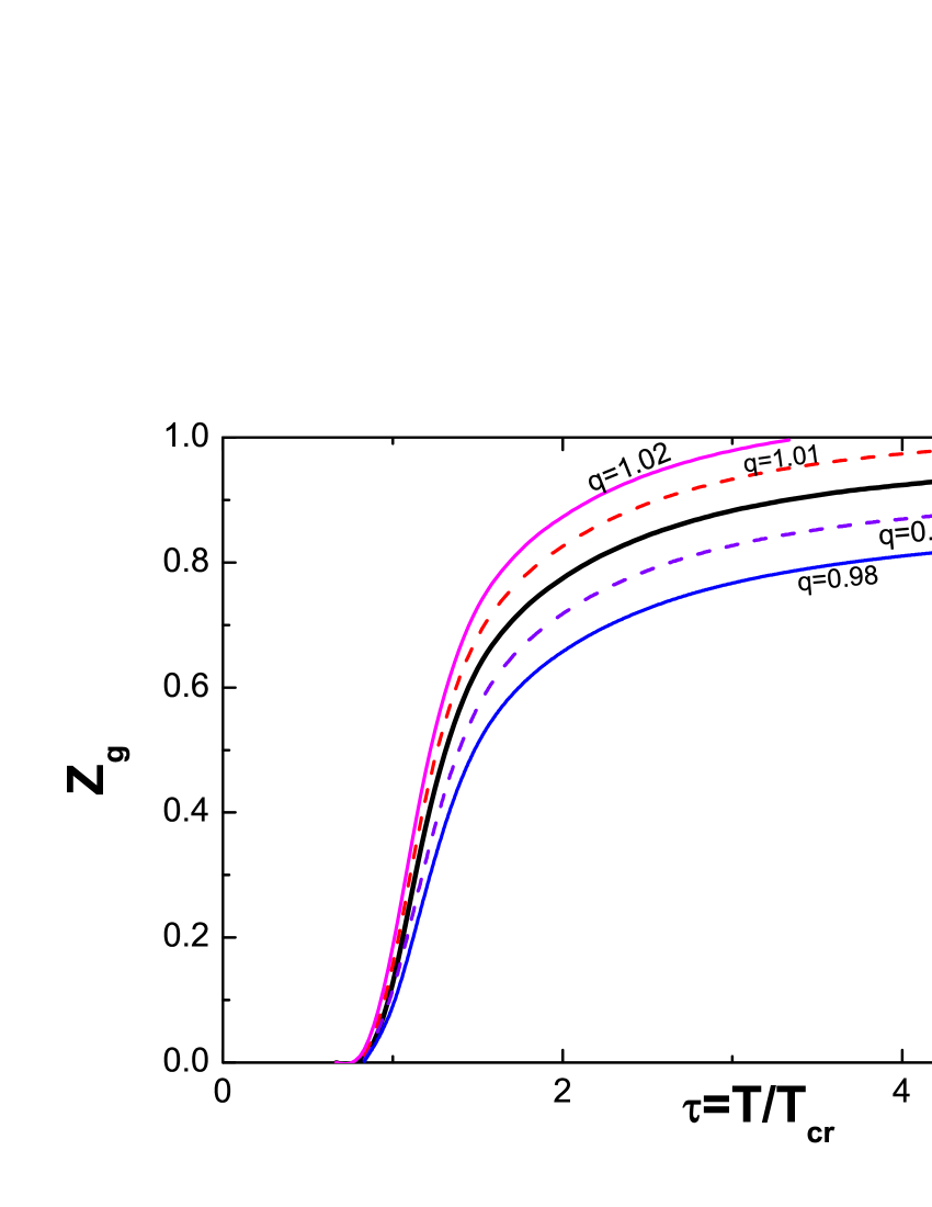
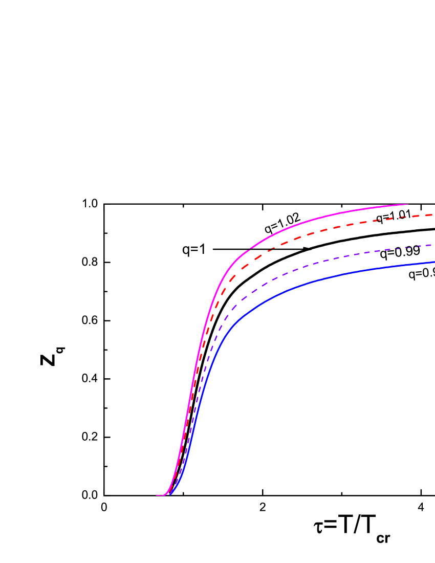
Figure 1: (Color online) Nonextensive effective fugacities $z_{q}^{(i)}$ for gluons ($i=g$, left panel) and quarks ($i=q$, right panel) plotted as functions of scaled temperature $\tau=T/T_{c}$ and obtained in approach $(B)$ (Eqs. (19) and (20)).

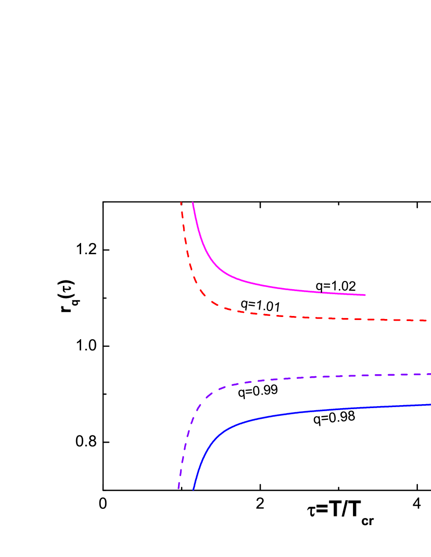
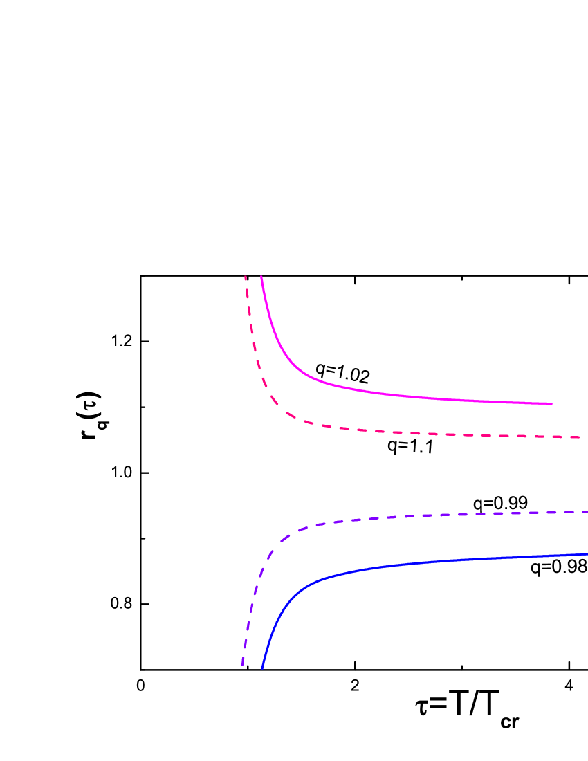
Figure 2: (Color online) The same $z_{q}^{(i)}(\tau)$ as presented in Fig. 1 but scaled by their corresponding extensive values (cf. Eq. (33)). The curves for $q=1.02$ end at $\tau$ for which corrresponding $z_{q}$ in Fig. 1 become unity.

We are therefore looking for values of the corresponding effective fugacities, $z_{q}^{(i)}(\tau)$, which in the nonextensive environment (i.e., on the rhs of Eq. (29)) should replace $z^{(i)}(\tau)$ in the extensive environment(i.e., on the lhs of Eq. (29)) in order to reproduce the lattice QCD data LQCD . Following CR1 this is done separately for the gluonic and quark sectors for which the following conditions must be satisfied:

$$\int_{0}^{\infty}dpp^{2}\ln[1-e\left(-\tilde{x}^{(g)}\right)]=$$

$$\,\,\,\,\,\,\,\,\,\,=\int_{0}^{\infty}dpp^{2}\ln_{2-q}\left[1-e_{2-q}\left(-x_{q}^{(g)}\right)\right],$$ (30)

for gluons and

$$\nu_{q}\int_{0}^{\infty}dpp^{2}\ln[1+e\left(-\tilde{x}^{(q)}\right)]+$$

$$\,\,\,\,\,\,\,\,\,\,+\nu_{s}\int_{0}^{\infty}dpp^{2}\ln[1+e\left(-\tilde{x}^{(s)}\right)]=$$

$$=\nu_{q}\int_{0}^{\infty}dpp^{2}\ln_{2-q}\left[1+e_{2-q}\left(-x_{q}^{(q)}\right)\right]+$$

$$\,\,\,\,\,\,\,\,\,\,+\nu_{s}\int_{0}^{\infty}dpp^{2}\ln_{2-q}\left[1+e_{2-q}\left(-x_{q}^{(s)}\right)\right],$$ (31)

for quarks; following CR1 , $\nu_{g}=16$, $\nu_{q}=24$ and $\nu_{s}=12$. The above equations provide us with $\tau$ and $q$-dependent relations between the extensive fugacities, $z^{(i)}(\tau)$ (which are our input), and nonextensive fugacities, $z_{q}^{(i)}(\tau)$ (which are our results).

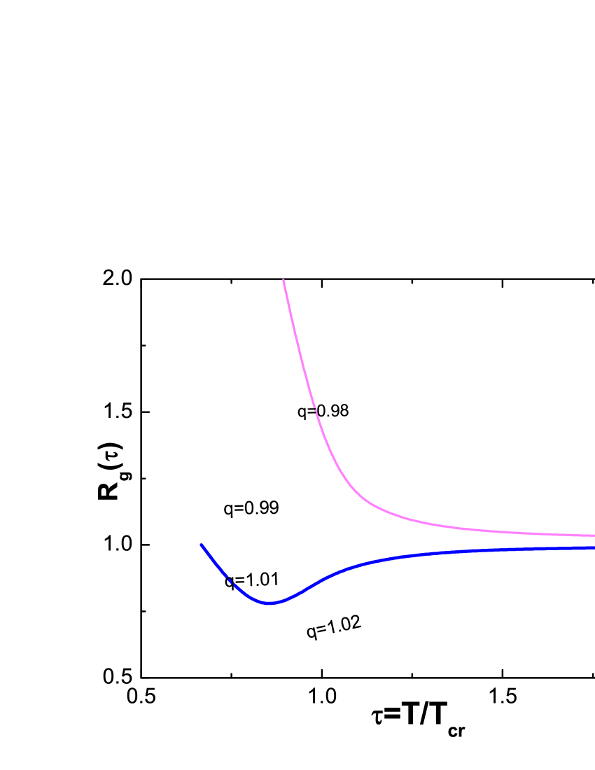
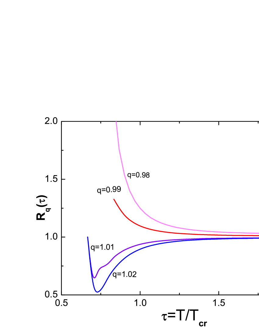
Figure 3: (Color online) Ratios $R(\tau)$ of gluonic fugacities (left panel) and quarkonic fugacities (right panel) calculated by methods $(A)$ and $(B)$ (cf. Eq. (34)) for $q=0.98$, $0.99$, $1.01$ and $1.02$ used above. For greater values of $\tau$ this ratio remains essentially unity.

As discussed in detail in CR1 , there is no one universal function describing the QCD data in the whole range of scaled temperatures $\tau$ used in fits; the cross-over point is at $\tau_{g}=1.68$ for gluons and $\tau_{q}=1.7$ for quarks. The low and high $\tau$ domains require different functional forms (the same occurs for quark and gluon sectors but with different parameters). Following CR1 we therefore take as our input:

$$z^{(g,q)} = a_{(g,q)}\exp\left[-b_{(g,q)}/\tau^{5}\right]\cdot\Theta\left(\tau_{(g,q)}-\tau\right)+$$ (32)

$$+ a^{\prime}_{(g,q)}\exp\left[-b^{\prime}_{(g,q)}/\tau^{2}\right]\cdot\Theta\left(\tau-\tau_{(g,q)}\right)$$

with $\left[a_{(g)},b_{(g)}\right]=(0.803,1.84)$, $\left[a^{\prime}_{(g)},b^{\prime}_{(g)}\right]=(0.98,0.94)$ for gluons and $\left[a_{(q)},b_{(q)}\right]=(0.81,1.72)$, $\left[a^{\prime}_{(q)},b^{\prime}_{(q)}\right]=(0.96,0.85)$ for quarks.

Fig. 1 shows the resulting $z_{q}{(i)}(\tau)$ (separately for gluons, $i=g$, and quarks, $i=q$) as functions of scaled temperature, $\tau=T/T_{c}$, calculated for approach $(B)$. Fig. (2) shows the same $z_{q}^{(i)}(\tau)$ but scaled by their corresponding extensive values, i.e., the ratios

$$r_{i}=r_{i}(\tau)=\frac{z_{q}^{(i)}(\tau)}{z_{q=1}^{(i)}(\tau)}.$$ (33)

The values of the nonextensivity parameter $q$ used here correspond to values of $q$ used by us before in the $q$ version of the Nambu Jona-Lasinio model JRGW .

The same can be calculated using method $(A)$. However, instead of repeating all the previous figures we simply present in Fig. 3 the corresponding ratios of results calculated using methods $(A)$ and $(B)$ (separately for gluons and quarks and as function of scaled temperature $\tau$),

$$R_{i}=R_{i}(\tau)=\frac{[z_{q}^{(i)}(\tau)]_{method(A)}}{[z_{q}^{(i)}(\tau)]_{method(B)}}.$$ (34)

Note the noticeable differences between both methods for smaller values of $\tau$ which tend to vanish for $\tau\geq 1.5$ .

The fugacities $z_{q}^{(i)}$ obtained above constitute our result. They demonstrate in a very clear way the action of immersing the QPM in a nonextensive environment with $q\neq 1$. They could be used for any further analysis based on the QPM, for example repeating the whole analysis of CR1 ; CR1a ; CR2 ; CRa3 ; CR3 for the $q\neq 1$ case. However, this is not our goal. We shall therefore end this section by presenting the physical significance of the effective nonextensive fugacities by presenting the corresponding nonextensive dispersion relations (i.e., single particle energies),

$$\varepsilon_{q}=-\frac{\partial}{\partial\beta}\left(\Xi_{q}\right).$$ (35)

In our case, for the first choice of $q$-QPM (Eqs. (5) and (16)), one gets

$$\varepsilon_{q}^{(i)}=E_{i}+T^{2}\frac{\partial\mu_{q}^{(i)}}{\partial T}=E_{i}+T^{2}\left[\frac{1}{z_{q}^{(i)}}\frac{\partial z_{q}^{(i)}}{\partial T}\right].$$ (36)

This means that for this form of the $q$-QPM extensivity affects only the interaction term. The quasiparticle energies get some additional contributions from their collective excitations. Note that this additional term occurs because of the temperature dependence of the effective fugacities and that it can be interpreted as representing the action of the gap equation in JRGW (but with constant energy $E_{i}$).

For the second choice of $q$-QPM (Eqs. (18) - (20)) one gets

$$\varepsilon_{q}^{(i)} = E_{q}^{(i)}+T^{2}\cdot\frac{\partial\ln_{2-q}\left(z_{q}^{(i)}\right)}{\partial T}=$$ (37)

$$= E_{q}^{(i)}+T^{2}\cdot\frac{1}{\left[z_{q}^{(i)}\right]^{q}}\frac{\partial z_{q}^{(i)}}{\partial T},$$

with $E_{q}^{(i)}$ given by Eq. (20). It means that for this form of the $q$-QPM both the initial energy and the interaction term are modified by effects of nonextensivity. As before, all modifications occur because of the temperature dependence of the effective fugacities and can be interpreted as representing action of gap equation in JRGW . However, now this representation is more exact because the energy $E_{i}$ is modified, cf., Eq. (20), and becomes the $q$-dependent quantity JRGW .

4 Summary and conclusions

This work illustrates how nonextensive environment (modelled by using $q$-exponentials and methods of nonextensive thermodynamics) changes usual extensive calculations. The quasiparticle model CR1 ; CR1a ; CR2 ; CRa3 ; CR3 used here as basis of our comparison allows for apparently maximal possible separation of effects of the usual dynamics (represented by fugacity $z$) from the effects caused by the nonextensive environment (represented by the nonextensivity parameter $q$). We have limited ourselves to investigation of the respective fugacities in two possible realization of the nonextensive version of the quasiparticle model, the $q$-QPM. They differ by the starting point assumed:

• in method $(A)$ it is gas of free, noninteracting quasiparticles immersed in extensive environment (i.e., free particles with interaction modelled by some assumed fugacities);

• in method $(B)$ it is gas of free particles immersed in nonextensive environment.

The main results are presented in Fig. 1. It is clearly visible that immersing free quasiparticles in some nonextensive environment described by the nonextensivity parameter $q>1$ considerably accelerates approach to the free (nonextensive) quasipartile limit of $z_{q}=1$. In the case of $q<1$ nonextensive environment this regime is practically never reached. Considering this result a comment concerning comparison with the similar nonextensive Nambu - Jona-Lasinio results JRGW are in order. As shown there, nonextensive effects result, for $q>1$, in the enhancement of the growth of pressure and entropy observed in the critical region of phase transition from quark matter to hadronic matter in lattice calculations for finite temperature Bazavov . As a result, for $q>1$ one reaches earlier the limit of noninteracting particles (albeit still remaining in a nonextensive environment), which corresponds to limit $z_{q}=1$ here (whereas there is no such transition for the $q<1$ case). Note that such limit is the same for quarks and gluons.

Finally, out of two methods of formulating the $q$-QPM presented here, method $(B)$ seems to be more complete and adequate in what concerns the introduction and description of the nonextensive effects. It can therefore be used further to investigate some more complicated aspects of dense matter in a nonextensive quasiparticle approach.

Acknowledgment

This research was supported in part by the National Science Center (NCN) under contract DEC-2013/09/B/ST2/02897. We would like to thank warmly Dr Nicholas Keeley for reading the manuscript.

References

- (1) G. Wilk and Z. Włodarczyk, Eur. Phys. J. A 40, 299 (2009).
- (2) G. Wilk and Z. Włodarczyk, Eur. Phys. J. A 48, 161 (2012).
- (3) G. Wilk and Z. Włodarczyk, Entropy 17, 384 (2015).
- (4) G. Wilk and Z. Włodarczyk, Chaos Solitons and Fractals 81, 487 (2015).
- (5) G. Wilk and Z. Włodarczyk, Acta Phys. Pol. B 46, 1103 (2015).
- (6) C. Tsallis, Introduction to Nonextensive Statistical Mechanics (Springer, Berlin, 2009).
- (7) C. Tsallis, Contemporary Physics, 55, 179 (2014).
- (8) C. Tsallis, Acta Phys. Pol. B 46 (2015) 1089. For an updated bibliography on this subject, see http://tsallis.cat.cbpf.br/biblio.htm;
- (9) A. P. Santos, F. I. M. Pereira, R. Silva and J. S. Alcaniz, J. Phys. G 41, 055105 (2014).
- (10) J. Rożynek and G. Wilk, Eur. Phys. J. A 52, 13 (2016).
- (11) E. Megias, D. P. Menezes and A. Deppman, Physica A 421, 15 (2015).
- (12) A. Deppman, J. Phys. G 41, 055108 (2014).
- (13) A. Lavagno, D. Pigato, Physica A 392, 5164 (2013).
- (14) J. Rożynek, Physica A 440, 27 (2015).
- (15) J. D. Walecka, Ann. Phys. 83, 491 (1974).
- (16) S. A. Chin and J. D. Walecka, Phys. Lett. B 52, 1074 (1974).
- (17) B. D. Serot and J. D. Walecka, Adv. Nucl. Phys. 16, 1 (1986).
- (18) Y. Nambu and G. Jona-Lasinio, Phys. Rev. 122, 345 (1961).
- (19) Y. Nambu and G. Jona-Lasinio, Phys. Rev. 124, 246 (1961).
- (20) S. P. Klevansky, Rev. Mod. Phys. 64, 649 (1992);
- (21) P. Rehberg, S. P. Klevansky and J. Hüfner, Phys. Rev. C 53, 410 (1996).
- (22) V. Chandra and V. Ravishankar, Phys. Rev. D 84, 074013 (2011).
- (23) V. Chandra, Phys. Rev. D 84, 094025 (2011).
- (24) V. Chandra and V. Ravishankar, Phys. Rev. D 92, 094027 (2015).
- (25) V. Chandra and V. Ravishankar1, Eur. Phys. J. C 59, 705 (2009).
- (26) V. Chandra and V. Ravishankar1, Eur. Phys. J. C 64, 63 (2009).
- (27) M. Cheng et al., Phys. Rev. D 81, 054504 (2010).
- (28) T. S. Biró, K. M. Shen and B. W. Zhang, Physica A 428, 410 (2015).
- (29) A. Bazavov et al., Phys. Rev. D 80, 014504 (2009).