Spherical collapse of dark matter haloes in tidal gravitational fields

Abstract

We study the spherical collapse model in the presence of external gravitational tidal shear fields for different dark energy scenarios and investigate the impact on the mass function and cluster number counts. While previous studies of the influence of shear and rotation on $\delta_{\mathrm{c}}$ have been performed with heuristically motivated models, we try to avoid this model dependence and sample the external tidal shear values directly from the statistics of the underlying linearly evolved density field based on first order Lagrangian perturbation theory. Within this self-consistent approach, in the sense that we restrict our treatment to scales where linear theory is still applicable, only fluctuations larger than the scale of the considered objects are included into the sampling process which naturally introduces a mass dependence of $\delta_{\text{c}}$. We find that shear effects are predominant for smaller objects and at lower redshifts, i. e. the effect on $\delta_{\mathrm{c}}$ is at or below the percent level for the $\Lambda$CDM model. For dark energy models we also find small but noticeable differences, similar to $\Lambda$CDM. The virial overdensity $\Delta_{\mathrm{V}}$ is nearly unaffected by the external shear. The now mass dependent $\delta_{\mathrm{c}}$ is used to evaluate the mass function for different dark energy scenarios and afterwards to predict cluster number counts, which indicate that ignoring the shear contribution can lead to biases of the order of $1\sigma$ in the estimation of cosmological parameters like $\Omega_{\text{m}}$, $\sigma_{8}$ or $w$.

1 Introduction

Since a decade cosmological observations provide very tight constraints on the parameters allowed within a certain class of models. With this ever increasing precision it is necessary to provide robust and accurate model predictions for future experiments. Combined observations of type-Ia supernovae (e.g. Riess et al., 1998; Perlmutter et al., 1999), the cosmic microwave background (e.g. Komatsu et al., 2011; Planck Collaboration XIII, 2015), the Hubble constant and large-scale structure (e.g. Cole et al., 2005) show that the universe is spatially flat and expanding in an accelerated fashion. Assuming the symmetries of standard cosmology and General Relativity to be true, the accelerated expansion can be described by the cosmological constant $\Lambda$ or by introducing a fluid component, dubbed dark energy (see e.g. Copeland et al., 2006, for a review), with an equation of state $w<-1/3$, which in principle can vary with time. The cosmological constant corresponds to a constant equation of state $w=-1$. So far there is no significant evidence for any departure from $\Lambda$.

However, even though the constraints on $w$ are quite tight today, its time evolution is constrained rather poorly. Therefore it is possible to allow for temporal variations in the equation of state. Models described by a generic time-varying equation of state are referred to as dynamical dark energy models. Despite the intense theoretical effort in revealing the nature of dark energy, the fundamental origin of dark energy is still unknown, therefore the majority of the studies are based on phenomenological assumptions on the time evolution of the dark energy equation of state. Once this quantity is specified, all the properties of dark energy at the background level are known. From a theoretical point of view, time-varying equations of state can naturally be achieved within the framework of scalar fields. In these models, once their self-interaction potential is specified, the time evolution of the scalar field is obtained by solving a Klein-Gordon equation and as consequence also the corresponding equation of state can be evaluated. Under the generic term of scalar field models, we have many sub-classes, such as quintessence models, phantom models, $k$-essence, tachyon models and so forth. Quintessence and phantom models can be accommodated within the minimally-coupled model class and the equation of state can be either strictly greater than -1 (quintessence) or smaller (phantom). Dark energy models do not affect only the background evolution by changing the Hubble factor, but also the evolution of structures. In addition, even if sub-dominant, dark energy can possess perturbations for $w\neq-1$.

A promising tool to reveal the time evolution of dark energy observationally is the halo mass function, which enters for example in cluster counts (Sunyaev & Zeldovich, 1980; Majumdar, 2004; Diego & Majumdar, 2004; Fang & Haiman, 2007; Abramo et al., 2009; Angrick & Bartelmann, 2009) or weak lensing peak counts (Maturi et al., 2010; Maturi et al., 2011; Lin & Kilbinger, 2014; Reischke et al., 2016). The halo mass function deals with objects in the highly non-linear regime and therefore a method is needed to extrapolate the linearly evolved density to the non-linear one. This is usually done by using the spherical collapse model introduced by Gunn & Gott (1972) and later extended in several works (Fillmore & Goldreich, 1984; Bertschinger, 1985; Ryden & Gunn, 1987; Avila-Reese et al., 1998; Mota & van de Bruck, 2004; Abramo et al., 2007; Pace et al., 2010; Pace et al., 2014a). The model assumes perturbations to be spherically symmetric non-rotating objects which decouple from the background expansion and thus reach a maximum point of expansion after which they collapse. In principle they would collapse to a single point. However, in reality the kinetic energy due to the collapse is converted into random motions of the particles in the over-dense regions, such that an equilibrium situation (in the sense of virialized structure, Schäfer & Koyama, 2008) is created. This model is, despite its simplicity, rather successful.

It is therefore important to get some insight into the theoretical assumptions of this model and to extend it towards more realistic situations. Especially rotation and shear effects are important extensions to the collapse model. Mainly rotational effects have been described in Pace et al. (2014b) which delay the collapse due to centrifugal forces, thus delaying the collapse of structures leading to a larger over-density needed for virialized structures. As the collapse model assumes a homogeneous sphere, shear effects are usually neglected, however, there can also be shear effects in homogeneous spheres and as real structures form in over-dense regions, there there will be shear effects due to external tidal fields. Those, if small enough, would not violate the symmetry assumptions of the model. External shear automatically leads to a mass dependence of the fundamental parameter of the spherical collapse, the critical over-density $\delta_{\text{c}}$, as light and therefore smaller objects will feel higher fluctuations in the density field than heavy objects. In this paper we will investigate the influence of external shear effects and how it depends on the underlying cosmological model. To this end we calculate the shear directly from the underlying density field by using first order Lagrangian perturbation theory, i.e. the Zel’dovich approximation (Zel’Dovich, 1970). We set up a random process to sample shear values from the statistics of the underlying density field and investigate how this affects the collapse on different scales. This procedure has the advantage that we do not need to rely on phenomenological models, as we can instead calculate the tidal shear from first principles as it is for example also done in angular momentum correlations of large scale structure due to tidal torquing (Schäfer, 2009).

The structure of the paper is as follows. In section 2 we review the spherical collapse model and show the equations to be solved. In section 3 we introduce a statistical procedure to obtain tidal shear values for the collapse. This method is then used in section 4 to calculate the influence of the tidal shear on $\delta_{\text{c}}$ for the standard $\Lambda$CDM model which is later generalized to more complicated dark energy models in section 5. In section 6 and 7 we investigate the influence of shear effects on the mass function and on cluster counts due to the Sunyaev-Zel’dovich effect and how a negligence of tidal shear effects can bias measurements of cosmological parameters. We summarize our findings in section 8.

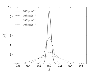
Figure 1: Normalized distribution of the density contrast $\delta=\psi_{ii}$ for different length scales. Note that we show the distribution of $\sigma_{\text{s}}^{2}$ with an offset of unity on the right. Clearly the values for $\delta$ below $R\approx 10\,\text{Mpc}h^{-1}$ would become too large in order to satisfy the assumption $\delta\ll 1$.

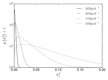
Figure 2: Normalized distribution of the tidal shear invariant $\sigma_{\text{s}}^{2}$ given in Eq. (12) for different length scales. Note that we show the distribution of $\sigma_{\text{s}}^{2}$ with an offset of unity on the right.

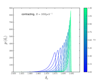
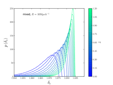
Figure 3: Distribution of $\delta_{\rm c}$ in over-dense regions at different redshifts for a radius $R=10\,\text{Mpc}h^{-1}$. Left: Contracting regions, i.e. regions with only positive eigenvalues of the velocity divergence tensor. Right: Regions which are partially expanding and partially contracting.

2 The Spherical Collapse Model

The spherical collapse model has been discussed by various authors, e.g Bernardeau (1994); Padmanabhan (1996); Ohta et al. (2003, 2004); Abramo et al. (2007) and Pace et al. (2010); Pace et al. (2014a). Here we start with the hydrodynamical equations

$$\begin{split}\dot{\delta}+(1+\delta)\nabla_{\boldsymbol{x}}\boldsymbol{u}=&\ 0\;,\\ \dot{\boldsymbol{u}}+2H\boldsymbol{u}+(\boldsymbol{u}\cdot\nabla_{\boldsymbol{x}})\boldsymbol{u}=&\ -\frac{1}{a^{2}}\nabla_{\boldsymbol{x}}\phi\;,\\ \nabla^{2}_{\boldsymbol{x}}\phi=&\ 4\pi Ga^{2}\rho_{0}\delta\;,\end{split}$$ (1)

with comoving coordinate $\boldsymbol{x}$, comoving peculiar velocity $\boldsymbol{u}$, Newtonian potential $\phi$, overdensity $\delta$ and background density $\rho_{0}$. The dot represents a derivative with respect to cosmic time $t$. Taking the divergence of the Euler equation and inserting the Poisson equation yields

$$\begin{split}\dot{\delta}=&-(1+\delta)\theta\;,\\ \dot{\theta}=&-2H\theta-4\pi G\rho_{0}\delta-\frac{1}{3}\theta^{2}-(\sigma^{2}-\omega^{2})\;,\end{split}$$ (2)

where we used the decomposition

$$\nabla_{\boldsymbol{x}}\cdot[(\boldsymbol{u}\nabla_{\boldsymbol{x}})\boldsymbol{u})]=\frac{1}{3}\theta^{2}+\sigma^{2}-\omega^{2}\;,$$ (3)

with the expansion $\theta=\nabla_{\boldsymbol{x}}\cdot\boldsymbol{u}$, the shear $\sigma^{2}\equiv\sigma_{ij}\sigma^{ij}$ and the rotation $\omega^{2}\equiv\omega_{ij}\omega^{ij}$. The rotation and the shear tensors are themselves the antisymmetric and the symmetric traceless part of the velocity divergence tensor, respectively. They are defined as

$$\begin{split}\sigma_{ij}=&\ \frac{1}{2}\left(\partial_{i}u_{j}+\partial_{j}u_{i}\right)-\frac{\theta}{3}\delta_{ij}\\ \omega_{ij}=&\ {\frac{1}{2}}\left(\partial_{i}u_{j}-\partial_{j}u_{i}\right),\end{split}$$ (4)

where $\partial_{i}\equiv\partial/\partial x^{i}$. We now use the relation $\partial_{t}=aH(a)\partial_{a}$ and $f\equiv 1/\delta$ which leads to

$$\begin{split}f^{\prime}=&\ \frac{\theta}{aH}f(1+f)\;,\\ \theta^{\prime}=&-\frac{2\theta}{a}-\frac{3H\Omega_{\text{m}}}{2af}-\left(\frac{1}{3}\theta^{2}+\sigma^{2}-\omega^{2}\right)\frac{1}{aH}\;.\end{split}$$ (5)

The system in Eq. (5) is solved numerically until $f\sim 10^{-14}$ and then it is extrapolated to zero. This yields the appropriate initial conditions for the linear evolution of the density contrast which gives $\delta_{\rm c}$. In the classical spherical collapse model, $\sigma^{2}$ and $\omega^{2}$ are neglected. However, their influence has been investigated by Del Popolo et al. (2013a, b) in the $\Lambda$CDM and dark energy cosmologies and by Pace et al. (2014b) in clustering dark energy models. The authors employ a heuristic model for the term $\sigma^{2}-\omega^{2}$ which allows to study an isolated collapse including a (mass dependent) quantity $\alpha$, defined as the ratio between the rotational and the gravitational term. Quantitatively, the term is

$$\alpha=\frac{L^{2}}{M^{3}RG}\;,$$ (6)

where $L$ denotes the angular momentum of the spherical overdensity considered and $M$ and $R$ its mass and radius, respectively. The angular term is important for galaxies and negligible for massive clusters; in particular $\alpha\approx 0.05$ for $M\approx 10^{11}\leavevmode\nobreak\ {\rm M}_{\odot}\leavevmode\nobreak\ h^{-1}$ and of the order of $10^{-6}$ for $M\approx 10^{15}\leavevmode\nobreak\ {\rm M}_{\odot}\leavevmode\nobreak\ h^{-1}$. By defining the twiddled quantities $\tilde{\theta}=\theta/H$, $\tilde{\sigma}=\sigma/H$ and $\tilde{\omega}=\omega/H$, the combined contribution of the shear and rotation term can effectively be modeled by

$$\tilde{\sigma}^{2}-\tilde{\omega}^{2}=-\frac{3}{2}\alpha\Omega_{\rm m}\delta\;,$$ (7)

leading to the modified Euler equation

$$\tilde{\theta}^{\prime}+\left(\frac{2}{a}+\frac{H^{\prime}}{H}\right)\tilde{\theta}+\frac{\tilde{\theta}^{2}}{3a}+\frac{3}{2a}(1-\alpha)\Omega_{\rm m}\delta=0\;.$$ (8)

In the notation of this work, Eq. (8) reads

$$\tilde{\theta}^{\prime}+\left(\frac{2}{a}+\frac{H^{\prime}}{H}\right)\tilde{\theta}+\frac{\tilde{\theta}^{2}}{3a}+\frac{3}{2a}\frac{(1-\alpha)\Omega_{\rm m}}{f}=0\;.$$ (9)

As shown by the authors, the effect of the term $\tilde{\sigma}^{2}-\tilde{\omega}^{2}$ is to slow down the collapse and to decrease the number of objects. This effect is differential and depends on mass and on redshift. At high redshifts, modifications are small, while at low redshifts they are more substantial. In addition, we can appreciate the slowing of the collapse (now mass dependent) for low mass objects.

In this work we follow a complementary approach. Instead of trying to model the additional non-linear term, we will derive only the shear contribution from the statistics of the density field in linear perturbation theory, since at early times velocities decay rapidly and vorticity is not sourced in the linear regime. Hence a direct comparison with the work by Del Popolo et al. (2013a, b); Pace et al. (2014b) cannot be performed. Note, however that we can expect an opposite behaviour of the collapse, since it is well known (Angrick & Bartelmann, 2010) that the ellipsoidal collapse proceeds faster than the spherical collapse.

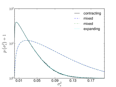
Figure 4: Distribution of the shear invariant $\sigma_{\text{s}}^{2}$ for different environments. We found that the mixed environment, i.e. where $\sigma_{ij}$ has positive and negative eigenvalues, is much more likely than the contracting or expanding environment making up for approximately $95\%$ of the sampled values. Note that we again show the normalized distribution with an offset of unity.

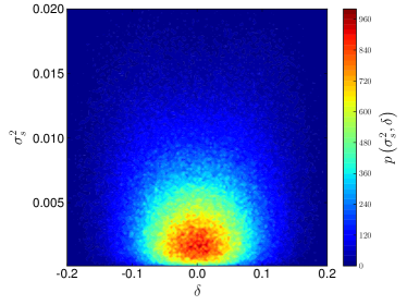
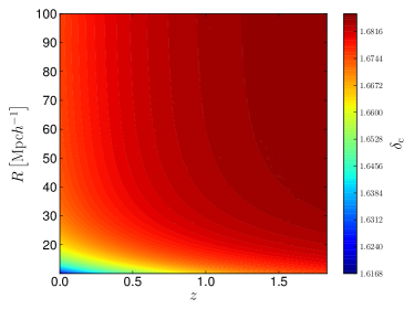
Figure 5: Left panel: Joint distribution of $\delta$ and $\sigma_{\text{s}}^{2}$ for a smoothing radius $R=30\;\text{Mpc}h^{-1}$. Right panel: Mean linearly evolved critical over-density $\bar{\delta}_{\text{c}}(M)$ including the shear as a function of redshift and object scale which is related to the mass of an object via $M=\frac{4\pi}{3}R^{3}\rho_{0}$, with $\rho_{0}=\rho_{\text{crit}}\Omega_{\text{m}}$. Clearly the effect of external shear is most pronounced at low redshifts and low masses, while it converges to the standard $\Lambda$CDM value for the other cases.

3 Sampling Tidal Shear Values

For the tidal shear we assume Zel’dovich velocities (Zel’Dovich, 1970), thus approximating the velocity field as a potential flow. For the trajectories one assumes

$$x_{i}=q_{i}-D_{+}(t)\partial_{i}\psi\equiv q_{i}-D_{+}(t)\psi_{,i}\;,$$ (10)

with the displacement field $\psi$ which is related to the density contrast $\delta$ via a Poisson relation, $\Delta\psi=\delta$, the initial position $q$ and the linear growth factor $D_{+}(t)$. The velocity is then given by

$$\dot{x}_{i}(t)=-\dot{D}_{+}(t)\psi_{,i}=-H\frac{\text{d}\ln D_{+}}{\text{d}\ln a}D_{+}\psi_{,i}\;.$$ (11)

Clearly there is no vorticity in this configuration, due to the permutability of the second derivatives. Thus the only remaining contribution to the spherical collapse is the traceless shear tensor

$$\sigma^{2}\equiv\sigma_{ij}\sigma^{ij}=\dot{D}_{+}^{2}(t)\left(\psi_{,ij}\psi^{,ij}-\frac{1}{3}(\Delta\psi)^{2}\right)\equiv\dot{D}_{+}^{2}(t)\sigma_{\text{s}}^{2}\;,$$ (12)

with $\psi_{,ij}\equiv\partial_{i}\partial_{j}\psi$. In the last step the time evolution was separated from the constant shear $\sigma_{\text{s}}^{2}$. We now sample values for the shear, $\psi_{,ij}$ directly from the statistics of the underlying density field. To this end we transform to Fourier space and use Poisson’s equation leading to

$$\psi_{,ij}=\int\frac{\text{d}^{3}k}{(2\pi)^{3}}\frac{k_{i}k_{j}}{k^{2}}\delta(\boldsymbol{k})\exp(\text{i}\boldsymbol{k}\boldsymbol{x})\;.$$ (13)

However, the correlation between the density field and the tidal shear is complicated in these coordinates. Following Regős & Szalay (1995) and Heavens & Sheth (1999) we consider the density peaks symmetric about the origin on the $z$-axis and introduce dimensionless complex variables

$$y^{n}_{lm}=\sqrt{4\pi}\frac{\text{i}^{l+2n}}{\sigma_{l+2n}}\int\frac{\text{d}^{3}k}{(2\pi)^{3}}k^{l+2n}\delta(\boldsymbol{k})Y_{lm}(\hat{k})\exp(\text{i}\boldsymbol{k}\boldsymbol{x})\;,$$ (14)

with the direction vector $\hat{k}=\boldsymbol{k}/k$ and $\sigma_{i}$ being the spectral moments of the matter power spectrum

$$\sigma_{i}^{2}=\frac{1}{2\pi^{2}}\int\text{d}k\;k^{2i+2}P(k),$$ (15)

while $Y_{lm}$ are spherical harmonics. We obtain a linear relation (Schäfer & Merkel, 2012) between $y^{n}_{lm}$ and the tidal shear values $\psi_{,ij}$

$$\begin{split}\sigma_{0}y_{20}^{-1}=&\ -\sqrt{\frac{5}{4}}\left(\psi_{,xx}+\psi_{,yy}-2\psi_{,zz}\right)\;,\\ \sigma_{0}y^{-1}_{2\pm 1}=&\ -\sqrt{\frac{15}{2}}\left(\psi_{,xz}\pm\text{i}\psi_{,yz}\right)\;,\\ \sigma_{0}y^{-1}_{2\pm 2}=&\ \sqrt{\frac{15}{8}}\left(\psi_{,xx}-\psi_{,yy}\pm 2\text{i}\psi_{,xy}\right)\;,\\ \sigma_{0}y^{0}_{00}=&\ \left(\psi_{,xx}+\psi_{,yy}+\psi_{,zz}\right)\;.\end{split}$$ (16)

In particular, the covariance in this basis is trivial, since the auto-correlation matrix is diagonal in $l$ and $m$:

$$\left\langle y_{lm}^{n}(\boldsymbol{x})y_{l^{\prime}m^{\prime}}^{n^{\prime}}(\boldsymbol{x})^{*}\right\rangle=(-1)^{n-n^{\prime}}\frac{\sigma^{2}_{l+n+n^{\prime}}}{\sigma_{l+2n}\sigma_{l+2n^{\prime}}}\delta_{ll^{\prime}}\delta_{mm^{\prime}}\;.$$ (17)

Thus, in the $y^{n}_{lm}$ basis the tidal shear values are uncorrelated Gaussian random variables with unit variance. We obtain the tidal shear values in physical coordinates by inverting the mapping

$$\sigma_{0}\boldsymbol{\alpha}=M\boldsymbol{\psi}\;,$$ (18)

where the six dimensional vectors $\boldsymbol{\alpha}$ and $\boldsymbol{\psi}$ bundle the variables in spherical and physical coordinates from Eq. (16) respectively

$$\begin{split}\boldsymbol{\alpha}^{\text{T}}=&\ \left(y_{00}^{0},y_{20}^{-1},y_{21}^{-1},y_{2-1}^{-1},y_{22}^{-1},y_{2-2}^{-1}\right)\;,\\ \boldsymbol{\psi}^{\text{T}}=&\ \left(\psi_{,xx},\psi_{,yy},\psi_{,zz},\psi_{,xy},\psi_{,xz},\psi_{,yz}\right)\;.\end{split}$$ (19)

The inverse mapping $M^{-1}$ is then given by

$$M^{-1}=\begin{pmatrix}1/3&-\frac{\sqrt{5}}{15}&0&0&\frac{\sqrt{30}}{30}&\frac{\sqrt{30}}{30}\\ 1/3&-\frac{\sqrt{5}}{15}&0&0&-\frac{\sqrt{30}}{30}&-\frac{\sqrt{30}}{30}\\ 1/3&2\frac{\sqrt{5}}{15}&0&0&0&0\\ 0&0&0&0&-\frac{\sqrt{30}}{30}\text{i}&\frac{\sqrt{30}}{30}\text{i}\\ 0&0&-\frac{\sqrt{30}}{30}&-\frac{\sqrt{30}}{30}&0&0\\ 0&0&\frac{\sqrt{30}}{30}\text{i}&-\frac{\sqrt{30}}{30}\text{i}&0&0\end{pmatrix}$$ (20)

Note that the components $y^{i}_{l\pm m}$ are Hermitian conjugate variables, thus preserving the real nature of the shear field. The amount of tidal shear acting on a halo depends on the length scale $R(M)$ of the halo and thus on its mass. In our model a halo will only be affected by the shear caused by structures with length scale $L\gtrsim R(M)$. Therefore we introduce a cut-off for the power spectrum, suppressing high frequencies

$$P(k)\to P(k)W^{2}_{R}(k),$$ (21)

with $W_{R}(k)=\exp(-k^{2}R^{2}/2)$. The mass scale is obtained via $M=\frac{4\pi}{3}\rho_{\text{crit}}\Omega_{\text{m}}R^{3}$, where $\rho_{\text{crit}}=3H^{2}/(8\pi G)$ is the critical density. Here all quantities are evaluated today, as the time dependence is taken into account via the time derivative of the growth factor in Eq. (10). From the sampled shear values $\psi_{,ij}$ the shear invariant $\sigma^{2}$ can be calculated using Eq. (12).

Clearly for low mass haloes shear becomes more important as the fluctuations in the surrounding density field are larger. Since our model works with a potential flow for the velocities, the variance $\sigma_{0}$ must remain small compared to $|\delta|=1$, showing the validity of the treatment presented here above a certain scale only on which the evolution of the density contrast can safely be considered as linear. In Figure 1 we show the distribution of the sampled density contrast $\delta=\psi_{ii}$ for different mass scales. It is easy to see that smoothing of the density field on smaller scales leads to a broader distribution of delta. Especially this shows that $R\approx 10\,\text{Mpc}h^{-1}$ is the smallest scale at which the approximation used here is applicable as higher order terms will dominate the perturbative expansion. Consequently the velocity field will no longer be a potential flow. Conversely larger scales $R(M)$ will lower the values of $\sigma_{\text{s}}^{2}$, thus high mass halos will be less affected compared to low mass ones. The distribution of the remaining tidal shear invariant $\sigma_{\text{s}}^{2}$ (cf. Eq. (12) for details), again for different scales, can be seen in Figure 2.

In Figure 4 we show how the invariant $\sigma^{2}_{\text{s}}$ distinguishes between different environments. These are classified by the characteristic of the shear tensor $\sigma_{ij}$. Due to $\Delta\psi=\delta$, positive eigenvalues correspond to a collapsing region, while negative eigenvalues correspond to an expanding region. The other two possibilities, i.e. one or two positive eigenvalues, correspond to a mix of both effects. Clearly the tidal shear invariant does not distinguish between contracting and expanding regions, as only the square of the traceless shear tensor enters into the collapse equation. The same is true for the mixed environments. Thus, a fully contracting environment has the same effect on the collapse as a fully expanding one. As halos form in over-dense regions, we are rather interested in a shear value provided the density contrast in this region satisfies $\delta>0$. It is important to note that no correlations enter into the model by conditionalizing the random process in such a way. The latter effect is shown in the right panel of Figure 4 where the joint distribution of $\sigma_{\text{s}}^{2}$ can be seen to be symmetric around $\delta=0$ for different values of $\sigma_{\text{s}}^{2}$ as expected from the Gaussian assumption and from Figure 1. It is therefore not harmful to neglect all values of the shear matrix which describe an under-dense region. Note that a halo can also form in a large under-dense region. Our results would, however, not be influenced by this effect as we work in the linear regime.

4 Effect of mass and environment

The critical linear over-density $\delta_{\rm c}$ in a homogeneous sphere depends on the initial conditions for the linear equation. Those are derived from the fully non-linear equation which in principle includes shear and rotation effects. Within our model $\delta_{\text{c}}$ will be influenced by the surrounding shear which is encapsulated in the invariant $\sigma_{\text{s}}^{2}$. As we have seen in Sect. 3 the shear values are distributed randomly due to the underlying density field with amplitudes given by the considered scale. Consequently $\delta_{\text{c}}$ will also exhibit a distribution rather than a distinct value.

The distribution of $\delta_{\text{c}}$ for different collapse redshifts can be seen in Figure 3. Contracting environments get less support by tidal shear than mixed environments which is due to the fact that the shear is larger if not all directions are contracting. The high end of both distributions falls off very rapidly which is due to the distribution $\sigma_{\text{s}}^{2}$ growing steeply towards $\sigma_{\text{s}}^{2}=0$. The zero point marks the value for $\delta_{\text{c}}$ obtained without tidal shear because $\sigma^{2}$ only enters as a positive contribution in Eq. (5) and thus a non-vanishing shear will move the initial conditions for the linear equation to lower values of $\delta$ resulting in a smaller value for $\delta_{\text{c}}$. Furthermore the distribution of $\delta_{\text{c}}$ becomes narrower if the collapse redshift increases. This is due to the evolution of $\sigma^{2}$ with redshift: physically shear becomes more important with time due to the growth of the cosmic density field. Note that this effect occurs only for $z$ larger than $0.3$ since the time evolution of $\sigma^{2}$ in Eq. (11) has a maximum at this redshift. It coincides with the time when the cosmological constant starts dominating the expansion of the universe, slowing down the growth of structures again.

Having evaluated the distribution of $\delta_{\text{c}}$ we can define an effective $\bar{\delta}_{\text{c}}$ which is taken to be the mean:

$$\bar{\delta}_{\text{c}}(M)=\int\text{d}\delta_{\text{c}}\;\delta_{\text{c}}\;p(\delta_{\text{c}},M).$$ (22)

This mean value is now a function of the mass of the considered halo, which is carried by the amplitude of the density fluctuations on scales larger than the corresponding scale $R(M)$ of the halo and of the redshift via the collapse equation. Figure 5 shows $\bar{\delta}_{\text{c}}$ as a function of the halo mass in units of $M_{\odot}h^{-1}$ and of the redshift. As expected from the previous discussion, $\delta_{\rm c}$ is mostly influenced at small radii and small redshifts as shear effects are most important in this regime.

5 Effect of cosmology

Previous works on the effects of shear and rotation on the parameters of the spherical collapse model showed that the behaviour of these additional non-linear terms is mildly affected by the change of the background cosmological model. While overall their mutual combination had the same qualitative effect (increase in $\delta_{\rm c}$ and negligible effect at high masses), differences of the order of several percent appeared across different cosmological models considered. In this section we analyse the effects of dark energy on the linear extrapolated density parameter $\delta_{\rm c}$ and on the virial overdensity when we add the contribution of the shear field as outlined in the previous sections. The models here investigated have been explored before with the same purpose, albeit, as said before, a direct comparison is not possible at this stage. For more details on the models we refer the reader to Pace et al. (2010) for homogeneous dark energy and to Pace et al. (2014b) for clustering dark energy models. We will explore the effect of dark energy inhomogeneities in a following work.

In particular we will explore the effect of the tidal shear in models described by the following equation-of-state parametrization: three models with constant equation of state ($w_{\rm DE}=-1$ for the cosmological constant $\Lambda$, $w_{\rm DE}=-0.9$ for quintessence models and $w_{\rm DE}=-1.1$ for phantom models), and six models with a dynamical equation of state:

• the 2EXP model (Barreiro et al., 2000),

• the CNR and the SUGRA model (Copeland et al., 2000),

• the CPL model (Chevallier & Polarski, 2001; Linder, 2003),

• the INV1 and INV2 models (Corasaniti & Copeland, 2003; Corasaniti, 2004; Sánchez et al., 2009).

In Figure 6 we show for clarity the dynamical dark energy models used in this work. The CPL and the INV2 models show a very gentle increase of the equation-of-state parameter while the models SUGRA and INV1 present a more rapid change of the equation of state. The CNR model is approximately constant at low redshifts and is characterized by a sudden change for $a\approx 0.1$. All the models are approximately constant at small scale factors and $w_{\rm DE}\approx-1$ for $a\simeq 1$, as inferred from observational data.

The functional form for the CPL model is

$$w_{\rm DE}(a)=w_{0}+w_{\text{a}}(1-a)\;,$$ (23)

and we used $w_{0}=-1$ and $w_{\text{a}}=0.15$.

The other models can be well described by the following four-parameter formula:

$$w_{\rm DE}=w_{0}+(w_{\mathrm{m}}-w_{0})\frac{1+e^{\frac{a_{\mathrm{m}}}{\Delta_{\mathrm{m}}}}}{1+e^{-\frac{a-a_{\mathrm{m}}}{\Delta_{\mathrm{m}}}}}\frac{1-e^{-\frac{a-1}{\Delta_{\mathrm{m}}}}}{1-e^{\frac{1}{\Delta_{\mathrm{m}}}}}\;.$$ (24)

In Table 1 we summarize the values of the parameters used.

Table 1: Parameter values for the dark energy models with dynamical equation-of-state parameter.

Model	$w_{0}$	$w_{\mathrm{m}}$	$a_{\mathrm{m}}$	$\Delta_{\mathrm{m}}$
2EXP	-0.99	0.01	0.19	0.043
INV1	-0.99	-0.27	0.18	0.5
INV2	-0.99	-0.67	0.29	0.4
CNR	-1.0	0.1	0.15	0.016
SUGRA	-0.99	-0.18	0.1	0.7

Except for the EdS model where we assumed $\Omega_{\rm m}=1$, we will use for all the dark energy models the following set of parameters (assuming a flat spatial geometry): $\Omega_{\rm m}=0.32$, $\Omega_{\rm de}=0.68$, $h=0.67$ and $n_{\rm s}=0.966$.

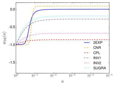
Figure 6: Time-dependent equations of state for the models used in this work as a function of the scale factor $a$. The light-green dashed-dot black and the magenta short-dashed lines represent the model INV1 and INV2, respectively. The blue curve the 2EXP model. The CPL and the CNR models are shown with the red dashed and the orange dashed curve, respectively. Finally the SUGRA model is shown with the cyan dotted curve.

5.1 Spherical collapse parameters

In this section we will describe the effects of the introduction of the tidal shear on the two main parameters of the spherical collapse model: the linearly extrapolated overdensity $\delta_{\rm c}$ and the virial overdensity $\Delta_{\rm V}$. The first one is a very important theoretical quantity usually used in the determination of the mass function according to the prescription of Press & Schechter (1974) and Sheth & Tormen (1999). The second one instead is used both in observations and in simulations to determine the mass and the size of the object. For details on how to evaluate them, we refer to Pace et al. (2010); Pace et al. (2012, 2014a); Pace et al. (2014b).

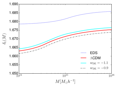
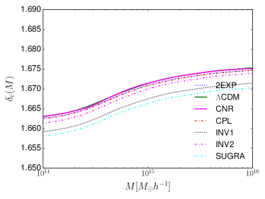
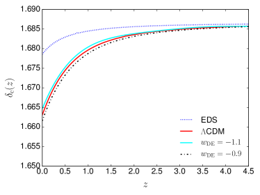
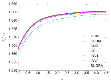
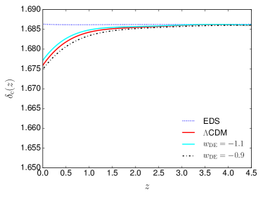
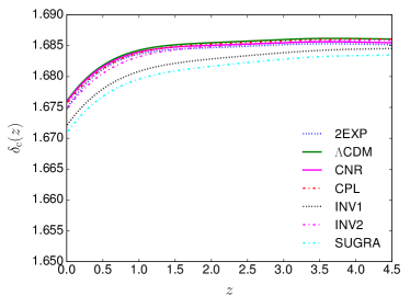
Figure 7: Upper panels: effects of the tidal shear on $\delta_{\rm c}$ at $z=0$ for different values of the mass of the collapsing sphere. Middle panels: time evolution of $\delta_{\rm c}$ for a mass of $M=10^{14}\leavevmode\nobreak\ M_{\odot}/h$. Bottom panels: time evolution of the linear extrapolated overdensity parameter for the standard spherical collapse model (without the inclusion of the tidal shear). Left (right) panels refer to constant (dynamical) equations of state. The red solid line refers to the reference $\Lambda$CDM model. For models with constant equation of state, the blue dotted curve shows an EdS model, while the black dashed-dot (cyan solid) curve shows a quintessence (phantom) model with $w_{\rm DE}=-0.9$ ($w_{\rm DE}=-1.1$). For dynamical dark energy models, the black dotted (magenta dashed-dot) curve represents the INV1 (INV2) model; the blue dashed curve the 2EXP model; the CPL (CNR) model with the red dashed-dot (magenta solid) curve and finally the SUGRA model with the cyan dashed-dot-dotted curve.

In Figure 7 we show our findings for the parameter $\delta_{\rm c}$ in several dark energy models, with respect to the $\Lambda$CDM model and to the respective values in absence of tidal shear. We refer the reader to the caption for the different colours and line-styles adopted for each model. In the left panels we show models with constant equation of state and in the right panels some dynamical models (i.e. with a time-varying equation-of-state parameter.)

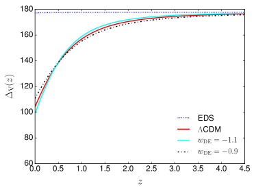
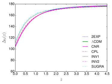
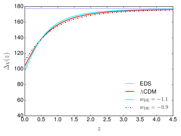
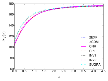
Figure 8: Upper panels: time evolution of $\Delta_{\rm V}$ for a mass of $M=10^{14}\leavevmode\nobreak\ M_{\odot}/h$. Bottom panels: time evolution of the virial overdensity for the standard spherical collapse model. Left (right) panels refer to constant (dynamical) equations of state. Line-styles and colours are as in Figure 7.

From a first qualitative analysis, results are as expected. Tidal shear favours the collapse and the linearly extrapolated overdensity parameter $\delta_{\rm c}$ is smaller than in the spherically symmetric case with no external tidal shear (compare the upper panels with values at $z=0$ in the bottom panels). The linear overdensity obviously depends on the halo mass now; stronger effects take place at low masses, at high masses the effect is negligible and the result converges to the standard spherically symmetric solution. This is particularly evident for the EdS model (blue dotted curve). Note however that differences from the standard case are quite small, below the 1% level. In the middle panel we fix the mass of the collapsing object at $M=10^{14}\leavevmode\nobreak\ M_{\odot}/h$, so to amplify the effect of the tidal shear, and we study the time evolution of the parameter $\delta_{\rm c}$. It is illuminating to compare it with the time evolution of the spherically symmetric case (bottom panel) and despite the results are not new since already derived and discussed previously in Pace et al. (2010), we report them once again for clarity. First of all notice that due to the tidal shear, for the EdS model $\delta_{\rm c}$ becomes time-dependent. Effects of the introduction of the ellipticity are more pronounced at low redshifts and they become negligible at high redshift, where the new solution converges to the standard value. Similar results, both qualitatively and quantitatively are obtained for generic dark energy models. All the models analysed show lower values for $\delta_{\rm c}$, especially at the lower end of the mass interval considered. At high masses values converge to the spherical case. Effects of the tidal shear are most evident at low redshifts and negligible at high redshifts. For $z\gtrsim 3$, the tidal shear contribution is totally negligible. Also for dynamical dark energy models, deviations from the standard case are below 1%.

In Figure 8 we present results for the virial overdensity parameter $\Delta_{\rm V}$. Interestingly, this quantity is insensitive to the introduction of the tidal shear and its time evolution is practically identical to what observed for the standard spherically symmetric case. This implies that for the virial overdensity, the solution of the standard theoretical model is an excellent approximation also for the case including the tidal shear. The reason why the results of the two approaches are identical, is due to the fact that the non-linear overdensity at turn-around, $\zeta$, is insensitive to the tidal shear. Also note that in general, differences between the dark energy models and the $\Lambda$CDM model are very limited.

Our results for $\delta_{\rm c}$ are qualitatively similar to the works of Del Popolo et al. (2013a) and Del Popolo et al. (2013b), albeit with some important differences and, as discussed before, with our formalism we can not do a quantitative comparison. First of all, $\delta_{\rm c}$ shows a mass dependence similar to the works mentioned. Effects of the modified collapse increase with decreasing mass and at the very high mass tail these modifications become negligible. Regarding the time dependence, also in our case larger modifications take place at low redshifts and at high enough $z$, the spherical case is an excellent approximation. In Del Popolo et al. (2013a) and Del Popolo et al. (2013b), the authors showed an increase in $\delta_{\rm c}$ rather than a decrease. However, in their heuristic model the dominant term was given by the rotation tensor, hence we would expect a slow-down of the collapse. It would be therefore interesting to find an approach, similar to what we did here, to take into account also the rotation term and then compare the two different approaches. The situation is completely different for the virial overdensity $\Delta_{\rm V}$: in our case it is totally independent of the tidal shear, hinting towards the hypothesis that probably the rotation is more important or that it is sensitive to the particular prescription adopted. Since the virial overdensity $\Delta_{\rm V}$ is largely independent of the tidal shear, it is interesting to examine why this happens. First of all it is useful to notice that our values for the tidal shear are much smaller than the ones used by Del Popolo and collaborators. To show this, it is sufficient to evaluate the relative strength of the shear term with respect to the Poisson term. In other words we are giving an estimate of the parameter $\alpha$ used in Del Popolo et al. (2013a, b). We find that in this work, $\alpha\simeq 10^{-8}$, while in previous works it was of the order of few per mill for an object of $10^{14}\leavevmode\nobreak\ \text{M}_{\odot}/h$.

To have a physical insight of this, we recall the definition of the virial overdensity. Note that we assume it with respect to the critical density, but the same result would apply if we would define it with respect to the background density. The virial overdensity is defined as

$$\Delta_{\rm V}=\zeta\left(\frac{x}{y}\right)^{3}\;,$$ (25)

where $\zeta=\delta(a_{\rm ta})+1$ is the overdensity at turn-around, $x=a/a_{\rm ta}$ is the scale factor normalised at the turn-around and finally $y=R_{\rm vir}/R_{\rm ta}$ is the virial radius normalized to the turn-around radius. As $\sigma^{2}$ enhances the collapse, $\zeta$ is smaller than the perfectly spherically symmetric case, as we need a smaller initial overdensity $\delta_{\rm i}$ to reach the collapse at $z_{\rm c}$. But $\zeta$ is evaluated only in the mildly non-linear regime, therefore it is only slightly smaller and the relative contribution of the $\sigma^{2}$ term compared to the Poisson term (the $\alpha$ coefficient) is to be about a few per mill at turn-around, in perfect quantitative agreement with our findings about the change of $\Delta_{\rm V}$.

On the other hand $z_{\rm ta}$ is slightly larger, but the effect is really small. The virialisation condition leading to $y=R_{\rm vir}/R_{\rm ta}$ does not directly depend on $\sigma^{2}$, but only indirectly via $z_{\rm ta}$. By Taylor expanding $\Delta_{\rm V}$ around the spherically symmetric case ($\sigma^{2}=0$), we have the following relations (the index 0 refers to the absence of shear):

$$\Delta_{\rm V}=\Delta_{\rm V,0}\left(1+\frac{\delta\zeta}{\zeta_{0}}+3\frac{\delta{z_{\rm ta}}}{1+z_{\rm ta,0}}-3\frac{\delta y}{y_{0}}\right)\;,$$ (26)

where, for a $\Lambda$CDM model at $z_{\rm c}=0$, we have:

$$\frac{\delta\zeta}{\zeta_{0}}\simeq-0.015\;,\quad\frac{\delta{z_{\rm ta}}}{1+z_{\rm ta,0}}\simeq 0.0014\;\quad\frac{\delta y}{y_{0}}\simeq-0.0047\;.$$

It is therefore clear that albeit extremely small, the dominant contribution is due to the change in $\zeta$, making as expected the virial overdensity only slightly smaller than in the spherical case.

It is also interesting to make a more direct comparison with the ellipsoidal collapse. One of the goals of this work is to establish whether a Press-Schechter formulation of the mass function with the corrections induced on $\delta_{\rm c}$ by the tidal shear tensor could give predictions closer to a Sheth-Tormen formulation with the standard $\delta_{\rm c}$ values. According to Bond & Myers (1996), the collapse time depends on the ellipticity $e$ and prolaticity $p$ and the dependence of the collapse threshold of an ellipsoidal region can be well approximated by the solution of (Sheth et al., 2001)

$$\frac{\delta_{\rm ec}}{\delta_{\rm sc}}=1+\beta\left[5(e^{2}\pm p^{2})\frac{\delta_{\rm ec}^{2}}{\delta_{\rm sc}^{2}}\right]^{\gamma}\;,$$ (27)

where $\delta_{\rm ec}$ and $\delta_{\rm sc}$ are the values of the critical overdensity for the ellipsoidal and spherical case, respectively and $\beta$ and $\gamma$ are parameters to be fitted to the results. Doroshkevich (1970) and Sheth et al. (2001) found that

$$\delta_{\rm ec}=\delta_{\rm sc}\left[1+\beta\left(\frac{\sigma(M)^{2}}{\delta_{\rm sc}}\right)^{\gamma}\right]\;,$$ (28)

with $\beta=0.47$ and $\gamma=0.615$. With $\sigma(M)$ of the order unity, $\delta_{\rm ec}$ is about 25% - 30% bigger than $\delta_{\rm sc}$. We can therefore conclude that the tidal shear will have small effects on the mass function, as shown later in Figure 9.

6 Mass function

The halo mass function describes the differential abundance of objects with mass $M$ at redshift $z$. Working within the theory of Gaussian random fields, the main ingredient is the comparison of fluctuations of the linearly evolved density field with $\delta_{\text{c}}$. Objects exceeding $\delta_{\text{c}}$ on a certain scale $R(M)$ are then counted as clusters. The fluctuations of the density field are described by the variance $\sigma_{R}$ of the underlying random field filtered with a top-hat having a certain scale. Press & Schechter (1974) showed that the mass function (PS) has the form

$$n(M,z)=\frac{2\rho_{0}}{\pi M}\frac{\delta_{\text{c}}(z)}{D_{+}\sigma_{R}}\left|\frac{\partial\ln\sigma_{R}}{\partial M}\right|\exp\left(-\frac{\delta_{\text{c}}^{2}(z)}{2D_{+}^{2}(z)\sigma_{R}^{2}}\right)\;,$$ (29)

where the growth factor $D_{+}$ accounts for the linear evolution. More elaborate forms of the mass function, fitting numerical $N$-body simulations better, are given in Sheth & Tormen (1999) or Jenkins et al. (2001). The important functional form for our purpose is however given by the term

$$\frac{\delta_{\text{c}}(z)}{D_{+}\sigma_{R}}\exp\left(-\frac{\delta_{\text{c}}^{2}(z)}{2D_{+}^{2}(z)\sigma_{R}^{2}}\right),$$ (30)

where we replace

$$\delta_{\text{c}}(z)\to\bar{\delta}_{\text{c}}(M,z)\;,$$ (31)

i.e. we insert the effective $\delta_{\text{c}}$. This has important consequences: Firstly, $\delta_{\text{c}}$ changes with the mass which will lead to a different form of the mass function. Furthermore, the shear causes $\delta_{\text{c}}$ to be smaller than without shear as it only supports the collapse. Due to the functional form of the mass function we therefore expect more massive haloes in the mass regime where the exponential factor dominates the linear one. On smaller scales, however, the linear term will dominate, thus causing the mass function to tend to smaller values. The reason for this behaviour is that small haloes can form more massive haloes more easily, thus yielding fewer smaller objects. Finally the time dependence of the shear is different from the linear growth of $\sigma_{\text{R}}$, we thus expect different impacts of the shear on different redshifts which in principle can make $\Lambda$CDM and $w$CDM models degenerate.

We now want to infer the influence of the tidal shear on the mass function for the several dark energy models analysed in this work. To do so, we evaluate the cumulative comoving number density of objects above a given mass at $z=0$. For all the models we assume $\sigma_{8}=0.776$. This is done not to introduce volume and normalization effects that would mask the contribution of the tidal shear, that, as we will see, amounts to few percent in a $\Lambda$CDM model.

We present our results in Figure 9, where we show the ratio between the dark energy and the reference $\Lambda$CDM model. In the left panels we show the ratio between the models with and without tidal shear field while in the right panels we show the ratio between the dark energy and the $\Lambda$CDM model with tidal shear field.

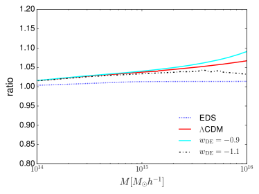
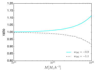
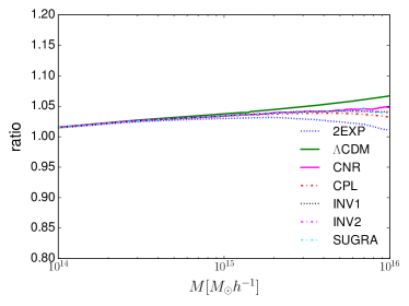
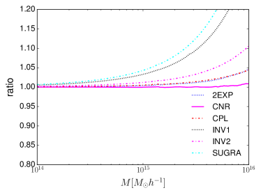
Figure 9: Ratio of the cumulative comoving number density of objects above mass $M$ evaluated at $z=0$. Left column: ratio between the expected number counts of the models with and without tidal shear contribution. Right column: ration between the dark energy and the $\Lambda$CDM model taking into account the effects of the tidal shear. Upper panels show results for the EdS model and dark energy models with constant equation of state ($w_{\rm DE}=-0.9$ and $w_{\rm DE}=-1.1$). Lower panels show results for dynamical dark energy models. Line-styles and colours are as in Figure 7.

By inspecting the left panels, we realize that, as expected, tidal shear has a modest contribution, usually growing with increasing mass. The effect is of the order of few percent at the lower limit of applicability of our formalism ($M\approx 10^{14}\leavevmode\nobreak\ M_{\odot}/h$) and it increases up to 10% for a model with constant $w_{\rm DE}=-0.9$ at very high masses ($M\approx 10^{16}\leavevmode\nobreak\ M_{\odot}/h$). The model being least affected is the EdS, somehow in agreement with what found for the spherical collapse parameter $\delta_{\rm c}$. Interestingly, the SUGRA model shows an increase with mass up to $M\simeq 10^{15}\leavevmode\nobreak\ M_{\odot}/h$ and a slow decrease to bring the model with tidal shear close to the standard one. Note that however differences are never bigger than about 3% for this model. Also note that, except for the model with constant $w_{\rm DE}=-0.9$, all the other models show an effect less pronounced in the high mass tail than the $\Lambda$CDM model and all the models, except for the EdS one, are identical to the $\Lambda$CDM model up to masses of $\simeq 10^{15}\leavevmode\nobreak\ M_{\odot}/h$.

In the right panels we show the ratio between the dark energy models and the $\Lambda$CDM one, both with the effects of the tidal shear field included. Results are both qualitatively and quantitatively as expected. For models with constant equation of state, the quintessence (phantom) model predicts more (less) objects with respect to the $\Lambda$CDM model and differences grow increasing the halo mass. All the dynamical dark energy models are in the quintessence regime and we see, as expected, more objects than the $\Lambda$CDM one. The CNR model behaves essentially as the $\Lambda$CDM model and the models CPL and 2EXP are practically indistinguishable and predict about 5% more objects than the $\Lambda$CDM one. Major differences arise for the SUGRA and the INV1 model.

The mass function described in Sheth & Tormen (1999) was introduced, as said above, to have a better match with $N$-body simulations. To do so, the authors incorporated the effect of shear in their calculations within the formalism of the ellipsoidal collapse model. The main quantity characterising the mass function is still the ratio $\delta_{\rm c}/D_{+}$ and effects due to the ellipsoidal collapse are incorporated directly in functional form of the mass function. We can therefore try to answer the following question: Will the Press-Schechter mass function approximate better the Sheth-Tormen mass function by using relation (31)? The idea behind that is in principle incorporating the tidal shear effects into the linear overdensity parameter and making it mass-dependent could compensate the necessity of modifying the functional form of the mass function. However, as one can see already in Figure 7, the influence on the mass function will only be a few percent. Accordingly it will of course improve the agreement between the Sheth Tormen mass function and the PS mass function, nonetheless this improvement is rather marginal with respect to the differences of the two mass functions at the high mass end. This can also be seen from the elliptical collapse model where the effective influence on $\delta_{\text{c}}$ is much larger than in our case leading to a big change in the number counts due to the exponential tail for massive objects including the collapse threshold (see subsection 5.1 for a more detailed discussion).

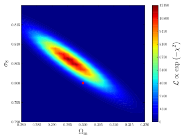
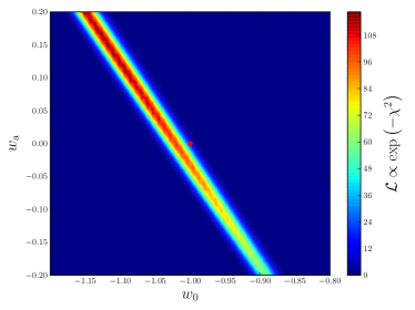
Figure 10: Bias on cosmological parameters for redshift cluster counts. Parameters not shown in the respective plot are fixed to their fiducial values. The red dot marks the fiducial cosmology with shear.

7 Cluster Counts

From the mass function, cluster counts can be calculated, which can then be compared to observational data. Using Sunyaev-Zel’dovich cluster surveys (Sunyaev & Zeldovich, 1980), the number of objects exceeding a mass $M_{\text{min}}$ in a redshift bin $z_{i}$ is given by (Majumdar, 2004)

$$N(z_{i})\equiv N_{i}=4\pi f_{\text{sky}}\int_{z_{i}-\Delta z_{i}/2}^{z_{i}+\Delta z_{i}/2}\text{d}z\frac{\text{d}V}{\text{d}z}\int_{M_{\text{min}}(z)}^{\infty}\text{d}M\;n(M,z)\;,$$ (32)

where $f_{\text{sky}}$ is the fraction of the sky. $M_{\text{min}}$ has a redshift dependence included. Assuming a Gaussian likelihood, the log-likelihood is given by $\chi^{2}$:

$$2{\chi^{2}}\equiv L=\sum_{i}\frac{(N_{i}-\langle N_{i}\rangle)^{2}}{N_{i}}\;,$$ (33)

where we sum over all redshift bins and Poisson errors are assumed. $\langle N_{i}\rangle$ is the model dependent expected number of objects in the $i$-th bin, while $N_{i}$ describes the data. We chose redshift bins with $\Delta z=0.02$ ranging from $z_{\text{min}}=0.01$ to $z_{\text{max}}=2$. For simplicity we assume $M_{\text{min}}=10^{14}h^{-1}M_{\odot}$ to be redshift independent. The mock data is sampled from a Poisson distribution with mean $N_{i}$ evaluated at the fiducial cosmology with $\Omega_{\text{m0}}=0.3$, $\Omega_{\Lambda}=0.7$, $\sigma_{8}=0.8$, $w_{0}=-1$ and $w_{\text{a}}=1$ and including shear effects in the mass function, cf. Eq. (31). A cosmological model without shear effects is fitted to this data, leading to biases in the cosmological parameters.

In Figure 10 we show the resulting biases in parameter space. The red dot marks the fiducial cosmology at which the data was sampled from a mass function including tidal shear via $\delta_{\text{c}}$. In contrast the black dot marks the best fit value of cosmological models without shear effects acting on $\delta_{\text{c}}$. Ignoring shear effects accordingly leads to wrong cosmological parameters, which are shifted by $\sim 1\sigma$ with respect to the true values for both $(\Omega_{\text{m}},\sigma_{8})$ and $(w_{0},w_{\text{a}})$.

8 Conclusion

In this work we investigated the influence of external tidal shear effects on the spherical collapse model using first order Lagrangian perturbation theory. The shear is evaluated directly from the statistics of the underlying density field in which the halo forms and therefore it does not need any further assumptions. Clearly, we cannot include rotational effects with our formalism, as the rotation vanishes identically for a potential flow, however for the scales investigated the assumption of linear growth is still valid, implying that, even if initial rotation was present (which would require third order Lagrangian perturbation theory) it would decay as the halo forms. In this sense our Ansatz for the shear is self-consistent.

In contrast, shear effects become more important for lower redshifts, as also the structures in the vicinity of the collapsing objects grow, thus increasing the curvature of the potential. We summarize our findings as follows:

1. External tidal shear supports the spherical collapse, which can be understood by noticing that virialized objects form in overdense regions in the first place. The effect is largest at small masses and low redshifts.

2. The effect on the important collapse parameter $\delta_{\text{c}}$ is of the percent level for both $\Lambda$CDM and more general dark energy models. Furthermore the influence on the virial overdensity $\Delta_{\text{V}}$ is very small and it is nearly indistinguishable from a collapse without external shear. The reason for this is mainly that the virial overdensity is basically evaluated using the time at turn-around. At this time the evolution is only in the mildly non-linear regime, therefore shear effects are not important.

3. Gaining a mass dependence due to our formalism, the influence on the mass function is two-fold. At lower masses the linear term dominates the exponential, suppressing the occurrence of lighter objects. Furthermore the influence of $\delta_{\text{c}}$ is largest at high masses, as the exponential tail dominates there. However, the effect of shear on $\delta_{\text{c}}$ becomes smaller for higher masses. The mentioned effects leads to a change of the mass function of roughly $2\%$.

4. The mass dependence translates into differences also in the cumulative number counts. Tidal shear affects number counts of massive halos of only few percent when compared to the corresponding model without it. When compared to the $\Lambda$CDM model with tidal shear, results are qualitatively and quantitatively the same as without tidal shear.

5. Neglecting the shear in the estimation of cosmological parameters using number counts, e.g. in redshift space, can lead to $1\sigma$ biases on cosmological parameters such as $\Omega_{\rm m}$, $\sigma_{8}$, $w_{0}$ and $w_{\text{a}}$.

6. The bias in the cosmological parameters is such that the inferred $\sigma_{8}$ ($\Omega_{\rm m}$) is higher (lower) than without and a $\Lambda$CDM model results into a dynamical phantom model for $a\approx 1$. The increase in $\sigma_{8}$ is in the right direction to at least alleviate the tension between the power spectrum normalization at late and early times, even if the amount is not sufficient. Remember however, that we neglected the rotation contribution and this could either balance or strengthen the shear contribution. Also the resulting phantom model is in agreement with SNIa observations, but at this stage we cannot draw any firm conclusion.

7. Previous works on the extended spherical collapse model introduced the effect of shear and rotation with heuristically motivated models (Del Popolo et al., 2013a). In this model, both shear and rotation are combined into a single term that depends on mass and result into a modification of the Poisson term, but the rotation term has a predominant role with respect to the shear. While a direct comparison cannot be made, our approach has some points in common and some major differences. While both approaches lead to a mass dependent spherical collapse, we find that effects of the shear are at percent level, contrary to what found in previous works. This leads to the question of the importance of the rotation and of its effective modelization.

References

- Abramo et al. (2007) Abramo L. R., Batista R. C., Liberato L., Rosenfeld R., 2007, Journal of Cosmology and Astro-Particle Physics, 11, 12
- Abramo et al. (2009) Abramo L. R., Batista R. C., Rosenfeld R., 2009, Journal of Cosmology and Astro-Particle Physics, 7, 40
- Angrick & Bartelmann (2009) Angrick C., Bartelmann M., 2009, Astronomy & Astrophysics, 494, 461
- Angrick & Bartelmann (2010) Angrick C., Bartelmann M., 2010, Astronomy & Astrophysics, 518, A38
- Avila-Reese et al. (1998) Avila-Reese V., Firmani C., Hernández X., 1998, ApJ, 505, 37
- Barreiro et al. (2000) Barreiro T., Copeland E. J., Nunes N. J., 2000, Phys. Rev. D, 61, 127301
- Bernardeau (1994) Bernardeau F., 1994, ApJ, 433, 1
- Bertschinger (1985) Bertschinger E., 1985, ApJS, 58, 39
- Bond & Myers (1996) Bond J. R., Myers S. T., 1996, ApJS, 103, 1
- Chevallier & Polarski (2001) Chevallier M., Polarski D., 2001, International Journal of Modern Physics D, 10, 213
- Cole et al. (2005) Cole S., et al., 2005, MNRAS, 362, 505
- Copeland et al. (2000) Copeland E. J., Nunes N. J., Rosati F., 2000, Phys. Rev. D, 62, 123503
- Copeland et al. (2006) Copeland E. J., Sami M., Tsujikawa S., 2006, International Journal of Modern Physics D, 15, 1753
- Corasaniti (2004) Corasaniti P. S., 2004, PhD thesis, University of Sussex, http://de.arxiv.org/pdf/astro-ph/0401517
- Corasaniti & Copeland (2003) Corasaniti P. S., Copeland E. J., 2003, Phys. Rev. D, 67, 063521
- Del Popolo et al. (2013a) Del Popolo A., Pace F., Lima J. A. S., 2013a, International Journal of Modern Physics D, 22, 50038
- Del Popolo et al. (2013b) Del Popolo A., Pace F., Lima J. A. S., 2013b, MNRAS, 430, 628
- Diego & Majumdar (2004) Diego J. M., Majumdar S., 2004, MNRAS, 352, 993
- Doroshkevich (1970) Doroshkevich A. G., 1970, Astrofizika, 6, 581
- Fang & Haiman (2007) Fang W., Haiman Z., 2007, Phys. Rev. D, 75, 043010
- Fillmore & Goldreich (1984) Fillmore J. A., Goldreich P., 1984, ApJ, 281, 1
- Gunn & Gott (1972) Gunn J. E., Gott III J. R., 1972, ApJ, 176, 1
- Heavens & Sheth (1999) Heavens A. F., Sheth R. K., 1999, Monthly Notices of the Royal Astronomical Society, 310, 1062
- Jenkins et al. (2001) Jenkins A., Frenk C. S., White S. D. M., Colberg J. M., Cole S., Evrard A. E., Couchman H. M. P., Yoshida N., 2001, MNRAS, 321, 372
- Komatsu et al. (2011) Komatsu E., Smith K. M., Dunkley J., et al. 2011, ApJS, 192, 18
- Lin & Kilbinger (2014) Lin C.-A., Kilbinger M., 2014, Proceedings of the International Astronomical Union, 10, 107
- Linder (2003) Linder E. V., 2003, Physical Review Letters, 90, 091301
- Majumdar (2004) Majumdar S., 2004, Pramana, 63, 871
- Maturi et al. (2010) Maturi M., Angrick C., Pace F., Bartelmann M., 2010, A&A, 519, A23
- Maturi et al. (2011) Maturi M., Fedeli C., Moscardini L., 2011, Monthly Notices of the Royal Astronomical Society, 416, 2527
- Mota & van de Bruck (2004) Mota D. F., van de Bruck C., 2004, A&A, 421, 71
- Ohta et al. (2003) Ohta Y., Kayo I., Taruya A., 2003, ApJ, 589, 1
- Ohta et al. (2004) Ohta Y., Kayo I., Taruya A., 2004, ApJ, 608, 647
- Pace et al. (2010) Pace F., Waizmann J.-C., Bartelmann M., 2010, MNRAS, 406, 1865
- Pace et al. (2012) Pace F., Fedeli C., Moscardini L., Bartelmann M., 2012, MNRAS, 422, 1186
- Pace et al. (2014a) Pace F., Moscardini L., Crittenden R., Bartelmann M., Pettorino V., 2014a, MNRAS, 437, 547
- Pace et al. (2014b) Pace F., Batista R. C., Del Popolo A., 2014b, MNRAS, 445, 648
- Padmanabhan (1996) Padmanabhan T., 1996, Cosmology and Astrophysics through Problems
- Perlmutter et al. (1999) Perlmutter S., Aldering G., Goldhaber G., et al. 1999, ApJ, 517, 565
- Planck Collaboration XIII (2015) Planck Collaboration XIII 2015, ArXiv e-prints, 1502.01589,
- Press & Schechter (1974) Press W. H., Schechter P., 1974, ApJ, 187, 425
- Regős & Szalay (1995) Regős E., Szalay A. S., 1995, Monthly Notices of the Royal Astronomical Society, 272, 447
- Reischke et al. (2016) Reischke R., Maturi M., Bartelmann M., 2016, Monthly Notices of the Royal Astronomical Society, 456, 641
- Riess et al. (1998) Riess A. G., Filippenko A. V., Challis P., et al. 1998, AJ, 116, 1009
- Ryden & Gunn (1987) Ryden B. S., Gunn J. E., 1987, ApJ, 318, 15
- Sánchez et al. (2009) Sánchez A. G., Crocce M., Cabré A., Baugh C. M., Gaztañaga E., 2009, MNRAS, 400, 1643
- Schäfer (2009) Schäfer B. M., 2009, International Journal of Modern Physics D, 18, 173
- Schäfer & Koyama (2008) Schäfer B. M., Koyama K., 2008, Monthly Notices of the Royal Astronomical Society, 385, 411
- Schäfer & Merkel (2012) Schäfer B. M., Merkel P. M., 2012, Monthly Notices of the Royal Astronomical Society, 421, 2751
- Sheth & Tormen (1999) Sheth R. K., Tormen G., 1999, MNRAS, 308, 119
- Sheth et al. (2001) Sheth R. K., Mo H. J., Tormen G., 2001, MNRAS, 323, 1
- Sunyaev & Zeldovich (1980) Sunyaev R. A., Zeldovich I. B., 1980, ARA&A, 18, 537
- Zel’Dovich (1970) Zel’Dovich Y. B., 1970, A&A, 5, 84