Relevant parameters in models of cell division control.

Abstract

A recent burst of dynamic single-cell growth-division data makes it possible to characterize the stochastic dynamics of cell division control in bacteria. Different modeling frameworks were used to infer specific mechanisms from such data, but the links between frameworks are poorly explored, with relevant consequences for how well any particular mechanism can be supported by the data. Here, we describe a simple and generic framework in which two common formalisms can be used interchangeably: (i) a continuous-time division process described by a hazard function and (ii) a discrete-time equation describing cell size across generations (where the unit of time is a cell cycle). In our framework, this second process is a discrete-time Langevin equation with a simple physical analogue. By perturbative expansion around the mean initial size (or inter-division time), we show explicitly how this framework describes a wide range of division control mechanisms, including combinations of time and size control, as well as the constant added size mechanism recently found to capture several aspects of the cell division behavior of different bacteria. As we show by analytical estimates and numerical simulation, the available data are characterized with great precision by the first-order approximation of this expansion. Hence, a single dimensionless parameter defines the strength and the action of the division control. However, this parameter may emerge from several mechanisms, which are distinguished only by higher-order terms in our perturbative expansion. An analytical estimate of the sample size needed to distinguish between second-order effects shows that this is larger than what is available in the current datasets. These results provide a unified framework for future studies and clarify the relevant parameters at play in the control of cell division.

I Introduction

Today, quantitative data of single dividing cells across generations and lineages can be produced with high throughput and spatiotemporal resolution. Such improved data have enabled renewed investigation of microbiological phenomena, where, given the intrinsic stochasticity of these systems, approaches based on statistical physics play a primary role. One example is the decision mechanism by which a cell divides, which has a key role in its size determination.

Several important recent findings have progressed this field, which were obtained by joint use of theoretical models and experiments measuring cell size and division events dynamically. Namely, (i) interesting scaling behavior emerges for the distributions of key variables such as doubling times and cell sizes across conditions and species Kennard2016 ; Iyer-Biswas2014 ; Giometto2013 , suggesting the existence of universal parameters setting these variables; (ii) relations between fluctuations of different quantities, for example relations between cell size and doubling time fluctuations with the average growth rate Kennard2016 ; Taheri-Araghi2015 ; (iii) mechanisms of division control can be explored and inferred using theoretical models, formulated as stochastic processes (of different kinds) whose dynamic variables are cell size, time and division events Amir2014 ; Osella2014a ; Campos2014 ; Taheri-Araghi2015 ; Kennard2016 .

The last point is the most studied, due to its direct biological relevance. The data typically rule out controls based on pure size and time measurements Taheri-Araghi2015 ; Osella2014a ; Robert2014 ; Soifer2016 . Concerted control mechanisms where multiple variables (e.g., time and size) may enter jointly have been proposed Amir2014 ; Osella2014a . Several studies in E. coli Campos2014 ; Taheri-Araghi2015 and other microbes Deforet2015 ; Taheri-Araghi2015 ; Soifer2016 ; Tanouchi2015 have argued for a mechanism in which the size extension in a single cell cycle is nearly constant and independent of the initial size of the cell (sometimes called “adder” mechanism of division control). However, it is clear that the constant added size is not the only trend found in the data Campos2014 ; Taheri-Araghi2015 ; Iyer-Biswas2014a ; Jun2015 , and that it is not a neccessary and sufficient condition for the observed scaling behavior and fluctuation patterns Kennard2016 . More broadly, the question of how much a mechanism can be isolated and specified with available data is still open.

Additionally, existing studies so far have relied on different modeling approaches, and raise the need for a unified framework. Specifically, two dominant formalisms emerge. The first describes the continuous-time division process by a hazard function, defining the probability per unit time that a cell divides, as a function of the values of measurable variables such as initial and/or current size, incremental or multiplicative growth, and elapsed time from cell division. The second formalism describes cell size across generations as a discrete-time auto-regressive process, (where a unit of time is a cell cycle).

Here, we propose a unified framework linking explicitly these two formalisms and we pose the question of the general possibility to distinguish mechanisms from data. Our formalism specifies the precise conditions on the parameters imposed by the empirically found scaling properties. By expanding around the mean initial size or inter-division time (generalizing the approach of ref. Amir2014 ), we show explicitly how this framework describes a wide range of division control mechanisms, including combinations of time and size control, as well as control by constant added size. As we show by analytical estimates and numerical simulation, the available data are characterized with great precision by the first-order approximation of this expansion. Hence, a single dimensionless parameter defines the strength and the action of the division control. However, this parameter may emerge from several mechanisms, which are distinguished only by higher-order terms in our perturbative expansion. Finally, we estimate the sample size needed to distinguish between second-order effects, and show that it is close to but larger than the size of currently available datasets.

II Background

II.1 Theoretical description of division control.

Our description assumes exponential growth of the cell size $x(t)=x_{0}e^{\alpha t}$, which is well supported in the literature Iyer-Biswas2014 ; Taheri-Araghi2015 ; Campos2014 ; Osella2014a and, as in previous modeling frameworks, neglects fluctuations of the growth rate $\alpha$ Iyer-Biswas2014 ; Osella2014a ; Taheri-Araghi2015 . A cell divides at a size $x_{f}$, and divides into two cells of equal size $x_{f}/2$ (we thus do not consider the small fluctuations around binary fission, the process of filamentation and recovery, or species with non-binary division Schmoller2015 ; Osella2014a ; Jun2015 ).

A control mechanism defines the division size $x_{f}$. In absence of this control, fluctuations of cell size may grow indefinitely in time. The full information on division control is encoded by the function $p(x_{f}|x_{0},\alpha)$, the conditional probability that a cell, born at size $x_{0}$ and growing with a growth rate $\alpha$, divides at size $x_{f}$. Note that the growth-division process is defined by four variables $x_{0},x,t,\alpha$, with the constraint of exponential growth and the model assumption of negligibile fluctuations in $\alpha$. This allows different equivalent parametrization of the process. A quantity of intereset is the size at birth of a cell, followed across generations. Given the conditional probability $p^{i}_{b}(x_{0}|\alpha)$ of observing a cell at generation $i$ with initial size $x_{0}$, the following Chapman-Kolmogorov equation gives the same probability at the subsequent generation

$$p^{i+1}_{b}(x_{0}|\alpha):=2\int_{0}^{\infty}dy\ p(2x_{0}|y,\alpha)p^{i}_{b}(y|\alpha)\ ,$$ (1)

where $p(x_{f}|x_{0},\alpha)$ plays the role of a transition probability.

The assumption of exponential single-cell growth implies that in this process the noise on doubling times has a multiplicative effect. Consequently, it is useful to introduce the quantity $q=\log(x/x^{\ast})$, which measures logarithmic deviations in size. At this stage, $x^{\ast}$ is an arbitrary scale, necessary to make the argument of the logarithm dimensionless. This choice is convenient as the exponential growth maps into the linear relation $q(t)=q_{0}+\alpha t$. The mechanism of division control can be equivalently specified in terms of $q$, by introducing the transition probability

$$\rho(q_{f}|q_{0},\alpha):=x^{\ast}e^{q_{f}}p(x^{\ast}e^{q_{f}}|x^{\ast}e^{q_{0}},\alpha)\ .$$ (2)

The mechanism of division control, defined by $p(x_{f}|x_{0},\alpha)$, determines the stationary distribution (if it exists) of sizes observed in a steadily-dividing population or genealogy, denoted by $p^{*}$. The stationary distribution for interdivision times $t_{d}$ derives equivalently from the mechanism of division control. A change of condition, e.g., nutrients or temperature, corresponds to a change of the growth rate $\alpha$, which, on turn has an effect on division control. It is observed experimentally that the stationary distributions of both initial size and inter-division time, measured under different conditions, collapse when rescaled by their means Taheri-Araghi2015 ; Kennard2016 , as shown in Fig. 1. In the following, we will assume this scaling property, which implies some constraints on the control defined by $p(x_{f}|x_{0},\alpha)$ Kennard2016 .

II.2 Scaling laws for size and doubling-time distributions as a result of division control

We now derive explicitly the constraints on division control emerging from finite-size scaling, following ref. Kennard2016 . Numerous experimental studies Taheri-Araghi2015 ; Kennard2016 ; Iyer-Biswas2014 ; Trueba1982 have shown that for several bacterial species and conditions the steady-state distributions of initial (or final) sizes and doubling times of dividing cells collapse when rescaled by their means. For instance, in the case of the initial size distribution, the scaling condition reads

$$p^{\ast}_{b}(x_{0}|\alpha)=\frac{1}{\langle x_{0}\rangle_{\alpha}}F\left(\frac{x_{0}}{\langle x_{0}\rangle_{\alpha}}\right)\ ,$$ (3)

where we defined

$$\langle x_{0}\rangle_{\alpha}:=\int dx\ p^{\ast}_{b}(x|\alpha)x\ .$$ (4)

A similar equation applies to the inter-division time distribution using $\langle t_{d}\rangle_{\alpha}$, i.e., the average inter-division time conditional on a growth rate.

When the fluctuations of $\alpha$ are neglected, the collapse can be explained as a result of the division control, but does not by itself isolate a specific mechanism Kennard2016 . Specifically, the observed collapse of the doubling-time and initial-size distributions implies that the conditional distribution $p(x_{f}|x_{0},\alpha)$ (for a growth condition with a given mean growth rate) has to collapse when both variables are rescaled by $\langle x_{0}\rangle_{\alpha}$

$$p(x_{f}|x_{0},\alpha)=\frac{1}{\langle x_{0}\rangle_{\alpha}}G\left(\frac{x_{f}}{\langle x_{0}\rangle_{\alpha}},\frac{x_{0}}{\langle x_{0}\rangle_{\alpha}}\right)\ .$$ (5)

This calculation is discussed in Appendix A1. Another important constraint implied by the scaling of the doubling time distributions (Appendix A1) is that the product $\alpha\langle\tau\rangle_{\alpha}$, does not depend on the mean growth rate in a given condition $\alpha$, which is the familiar condition matching the population average of growth rate and with the inverse average doubling time.

Finally, Eq. (5) implies that the division control depends on a single “internal” size scale, which, in turn, sets the value of $\langle x_{0}\rangle_{\alpha}$. In conclusion, the joint universality in doubling time and size distributions can be explained by division control mechanisms based on a single length (size) scale and $1/\alpha$ as the unique time scale. While this condition does not imply any mechanism, it can be applied to different modeling frameworks, allowing model-independent predictions.

Figure 1: Finite-size scaling properties of cell size and the division-control function. A: Collapse of the probability distribution of rescaled logarithmic size $\log(x_{0}/\langle x_{0}\rangle_{\alpha})$ across different conditions/strains (colors) (equivalent to the condition in Eq. (3)). B: The function $f(\cdot)$ defining the mechanism of size control in the discrete-time Langevin framework (Eq. (7)) collapse when rescaled as predicted by Eq. (9). Data were obtained from refs. Kennard2016 and Wang2010a . Data from ref. Kennard2016 refer to two strains, P5-ori (a BW25113 derivative strain) and MRR, grown on agarose pads in four nutrient conditions (Glc, CAA, RDM and LB). Data from ref. Wang2010a (orange triangle) refer to MG1655 strain in a microfludic device with LB as growth medium.

III Results

III.1 A unified modeling framework connects different descriptions of the growth-division process.

We aim to provide a generic framework describing growth-division data, which can be compared with data and used to draw conclusions on the possible mechanism of division control. To this end, two main theoretical formalisms have been employed so far. The first describes cell growth and division as a continuous-time process in which the main parameter is time elapsed from the last cell division. The second describes the dynamics of measurable variables, such as initial size and interdivision time across generations, thus using the generation index as a discrete time. This section reviews the two frameworks, showing how they are equivalent, and explicitly providing the map connecting them. This map leads us to a discrete-time equation, where the function describing the control is mapped explicitly to a hazard rate. Finally, we show how this equation is constrained by the collapse of size and doubling-time distributions.

The continuous-time approach Osella2014a ; Taheri-Araghi2015 ; Painter1968 supposes an underlying “decisional process” for cell division, which is entirely specified by the dependency of the division rate $h_{d}$ from the measured dynamic parameters, such as cell instantaneous and initial size, added size, elapsed time from the previous cell division, and growth rate. The fuction $h_{d}$ is analogous to an hazard rate in survival models. In particular, since division control is fully specified by $p(x_{f}|x_{0},\alpha)$, one has the relation

$$p(x|x_{0},\alpha)=-\frac{d}{dx}\exp\left(\int_{0}^{x}ds\ h_{d}\left(s,x_{0},\alpha\right)\right)\ .$$ (6)

This function $h_{d}$ can be inferred directly from data or a specific functional form can be assumed to test specific model predictions Osella2014a . Previous work Taheri-Araghi2015 has shown that data are well reproduced by models where the division rate depends on added size $x-x_{0}$, or by more complex “concerted control” models where the rate is allowed to depend on two variables, instantaneous size $x$ and initial size $x_{0}$ or elapsed time $t$ (the latter two variables are essentially interchangeable since the distribution of elongation rates is generally quite peaked) Osella2014a . This approach works very well in reproducing essentially all available observations. However, it leads to the problem of finding an interpretation of $h_{d}$, which is not simple. In future studies, where $h_{d}$ can be linked to “molecular” variables such as concentrations or absolute amounts of cell-cycle related proteins this may become easier. The other problem with the approach is that $h_{d}$ is a function, and, while it can be inferred directly from data, its parameterization may be far from obvious.

In order to comply with the empirical scaling properties of initial, final and added size, and of interdivision time, the hazard rate function must collapse when both variables are rescaled by $\langle x_{0}\rangle_{\alpha}$ (see Eq. (5)),

$$h_{d}(x,x_{0},\alpha)=\tilde{h}\left(\frac{x}{\langle x_{0}\rangle_{\alpha}},\frac{x_{0}}{\langle x_{0}\rangle_{\alpha}}\right)\ .$$

The discrete-time formalism Amir2014 ; Soifer2016 ; Tanouchi2015 ; Taheri-Araghi2015 gives up the ambition of capturing doubling time fluctuations, in order to obtain a clearer view of the dynamics of cell size. Importantly, this approach makes an assumption for doubling time fluctuations, defining the doubling time conditional to a certain initial size $x_{0}$ as a random variable with a pre-defined mean $\tau_{0}$ and “noise” $\xi$, $\tau=\tau_{0}+\xi$, where the distribution of the zero-mean variable $\xi$ must be specified. One can verify a posteriori whether these assumptions are reasonable in data. This choice leads to discrete-time Langevin equations for the initial size $x_{0}(i)$ where $i$ is the cell-cycle index.

$$x_{0}(i+1)=f\left(x_{0}(i),\alpha\right)+\eta(x_{0}(i),\alpha)\ ,$$ (7)

where the function $f(\cdot)$ specifies cell division control, while $\eta$ is a random noise with mean zero and arbitrary distribution. In particular $f(\cdot)$ is given by

$$f\left(x_{0},\alpha\right)=\frac{1}{2}\int_{0}^{\infty}dx\ p(x|x_{0},\alpha)x\ .$$ (8)

Different forms of this function correspond to different kinds of controls on cell division. For instance a perfect sizer (division triggered by an absolute cell size $x^{\ast}$) corresponds to $f\left(x_{0},\alpha\right)=x^{\ast}$ while an adder (division triggered by a noisy constant added size) is defined by $f\left(x_{0},\alpha\right)=(x_{0}+\Delta)/2$.

The scaling relation in Eq. (5), imposes that $f\left(x_{0},\alpha\right)/\langle x_{0}\rangle_{\alpha}$ is solely a function of the ratio $x_{0}/\langle x_{0}\rangle_{\alpha}$. In particular, one can derive a simple relation between $f$ and the hazard rate function, obtaining

$$\begin{split}&\frac{1}{\langle x_{0}\rangle_{\alpha}}f\left(x_{0},\alpha\right)=\\ &=\frac{1}{2}\left(-\frac{x_{0}}{\langle x_{0}\rangle}+\int_{\frac{x_{0}}{\langle x_{0}\rangle}}^{\infty}dy\ \exp\left(\int_{y}^{\infty}dz\ \tilde{h}\left(z,\frac{x_{0}}{\langle x_{0}\rangle}\right)\right)\right)\ .\end{split}$$ (9)

This function can be estimated from empirical data as $f(x_{0},\alpha)=\langle x_{0}(i+1)\rangle_{x_{0}(i)=x_{0}}$, the average size at birth of the daughter conditional on the size at birth of the mother. Fig. 1B reports $f(x_{0}/\langle x_{0}\rangle_{\alpha})/\langle x_{0}\rangle_{\alpha}$ in empirical data for different growth conditions experiments and strains, showing the expected collapse.

Considering the discrete framework, we can write an equivalent process for the initial logarithmic size $q$, which, after having imposed the constraints given by the scaling of the stationary distribution, reads

$$q_{0}(i+1)=\bar{q}_{\alpha}+g\left(q_{0}(i)-\bar{q}_{\alpha}\right)+\xi(q_{0}(i)-\bar{q}_{\alpha})\ ,$$ (10)

where $\bar{q}_{\alpha}=\log(c\langle x_{0}\rangle_{\alpha}/x^{\ast})$, with $c$ being an arbitrary constant, and $g(\cdot)$ specifies cell division control in log-space, analgous to $f(\cdot)$ in Eq.(7). The noise term is again drawn from a zero-mean distribution. Also in this case we can write explicitly the form of $g$ given an hazard rate function $h_{d}(\cdot)$ (see Appendix A2). The function can be estimated from empirical data by evaluating $g(\Delta q)=\langle q_{0}(i+1)-\bar{q}_{\alpha}\rangle_{q_{0}(i)-\bar{q}_{\alpha}=\Delta q}$.

The two functions $f(\cdot)$ and $g(\cdot)$, appearing in Eq. (7) and (10) are interchangeable. Both expressions, once defined, correspond unequivocally to a specific division control mechanism. To obtain the hazard rate function, one must specify the distribution of the noise terms. Since in empirical data the initial and final size are approximately lognormally distributed Kennard2016 , the steady-state distribution of $q$ can be well approximated by a Gaussian. It is therefore reasonable to assume that the distribution of the noise is Gaussian itself

$$\Delta q_{0}(i+1)=g\left(\Delta q_{0}(i)\right)+\sigma\left(\Delta q_{0}(i)\right)\xi\ ,$$ (11)

where $\xi$ in this expression is a Gaussian random variable of zero mean and unit variance and $\sigma(\cdot)$ a proper function of $\Delta q_{0}(i)=q_{0}(i)-\bar{q}_{\alpha}$. Under this assumption, we obtain (see Appendix A2)

$$h_{d}(x,x_{0},\alpha)=\frac{1}{x}g_{\sigma}\left(\frac{\log(x/\langle x_{0}\rangle_{\alpha})-g\left(\log(x_{0}/\langle x_{0}\rangle_{\alpha})\right)}{\sqrt{2}\sigma(\log(x_{0}/\langle x_{0}\rangle_{\alpha}))}\right)\ ,$$

where

$$g_{\sigma}(y)=\frac{1}{\sqrt{2\pi}\sigma}\frac{\exp(-y^{2})}{1-\text{Erf}(y)}\ ,$$

where $\text{Erf}(\cdot)$ is the error function. Note that, however, for unspecified $g(\cdot)$ and $\sigma(\cdot)$, the stationary distribution of this process is not a Gaussian in general. Our direct calculation of the hazard rate $h_{d}$ from the control function $g$ links the discrete-time to the continuous-time formalism through a quantitative map. We will now focus on the parameterization defined in Eq. (11), showing how it can be reduced to a single relevant parameter, using a perturbative approach.

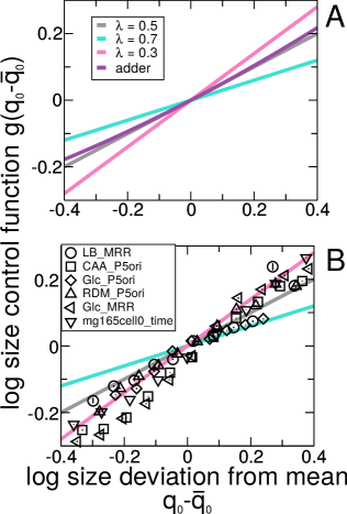
Figure 2: Unified framework of division control and comparison with data. A: Division control function $g(\cdot)$, for an adder model (purple solid line) and linearized models with different values of the control parameter $\lambda$ (cyan, grey, magenta solid lines). This function defines the control mechanism in the model (Eq. (10)). The adder mechanism is near linear and closest to the linearization with $\lambda\sim 0.5$ Amir2014 . B: Comparison between data (symbols) and the linearized discrete-time Langevin framework, for different values of the single control parameter $\lambda$. The roughly linear scaling of the symbols suggests that the data are close to a simple discrete-Langevin scenario, and the collapse across different strains and conditions confirms the results of Fig. 1. Values of $\lambda$ around $1/2$ well reproduce the data, but deviations are visible. Data (from ref.Kennard2016 and Wang2010a ) refer to different strains of dividing E. coli cells grown in different conditions (see Fig. 1).

III.2 A perturbative approach identifes the conditions for a steady-state size distribution (homeostasis)

We now consider a general perturbative expansion around the mean initial logarithmic size of the population, which unveils the relations between different simplified descriptions, and extends the approach of ref. Amir2014 . As we will see, it is possible to assign a simple interpretation to the coefficient of the expansion and use it to formulate physical considerations and estimates on the possible division control mechanisms. This kind of expansion is justified by empirical observations, as follows. The collapse of the initial-size distributions implies that the standard deviation $\sigma_{x_{0}}$ (which depends on the condition through the population growth rate $\alpha$), scales as $k\langle x_{0}\rangle_{\alpha}$, where $k$ is a constant independent of $\alpha$. The constant $k$, which is the coefficient of variation, has empirical values around $0.15$ Taheri-Araghi2015 . Such value implies that the fluctuations of sizes around their mean are small and suggests therefore to expand size fluctuations around the mean.

Instead of expanding the feedback control in powers of the ratio $\sigma_{x_{0}}/\langle x_{0}\rangle_{\alpha}$, we will focus on logarithmic size, i.e., the previously introduced variable $q$. Starting from Eq. (11), one can expand $g(\cdot)$ and $\sigma(\cdot)$ around $q_{0}(i)=\bar{q}_{\alpha}$. In this case, taking the first order of the expansion, we obtain

$$\Delta q_{0}(i+1)=(1-\lambda)\Delta q_{0}(i)+\sigma\xi\ ,$$ (12)

where $\lambda=1-g^{\prime}(0)$ and $\sigma=\sigma(0)$. The process defined by Eq. (11) is a discrete-time Langevin equation in a quadratic potential with stiffness $\lambda$, and thus can have multiple physical analogs. Its exact solution is a Gaussian distribution of $q_{0}$ with mean $\bar{q}_{\alpha}$ and variance $\sigma_{q}^{2}=\sigma^{2}/(\lambda(2-\lambda))$ (see Appendix A4 and ref. Amir2014 ), which correspond to a lognormal distribution of $x_{0}$. This relation can be considered as a discrete version of a fluctuation-dissipation theorem, as it connects the fluctuations of cell size $\sigma_{q}$ with the strength of the response $\lambda$ to deviation of the size from the mean.

Eq. (12) can be solved exactly. Starting from an arbitrary initial condition, we derive the distribution of sizes after any number of generations (Appendix A4). In particular, it is possible to calculate how fluctuations of size are dampened in time. Starting at generation $0$ with an initial size corresponding to $q_{0}(0)$, the expected size at birth after $n$ generations is

$$\langle\Delta q_{0}(n)\rangle=\Delta q_{0}(0)\left(1-\lambda\right)^{n}\ .$$ (13)

It is simple to see from this expression that, as expected, homeostasis is possible only if $|1-\lambda|<1$ and that $1<\lambda<2$ would lead to oscillatory sizes around the mean Tanouchi2015 . The role played by $\lambda$ is therefore to set the correlation time-scale, measured in generations.

Eq. (12) and (13) show that a steady-state size distribution (“size homeostasis”) is possible if $|1-\lambda|=|g^{\prime}(0)|<1$ (see Fig. 3A). This is a necessary condition, but not a sufficient one, as it only implies local stability of the deterministic solution (Appendix A3). While values of $\lambda$ between $1$ and $2$ guarantee homeostasis, current data suggests that they are not biologically relevant. A value larger than one would in fact correspond to an extra correction of the size, which controls fluctuations in a oscillatory way. In this case, if a cell has a size larger than the average, the daughter will have on average a size smaller than average but closer and the grand-daughter a size again larger than the average and so on. Since this behavior is not observed in experiments we restrict our analysis to the case $0<\lambda<1$.

Considering the next orders in the expansion, one can obtain precise criteria on the conditions leading to homeostasis. When only the deterministic part of Eq. (10) is considered (i.e. $\sigma=0$), it is possible to show that the equilibrium is unique and globally stable if $|g(\Delta q)|<|\Delta q|$. If the noise is additive (i.e., $\sigma(\Delta q)$ is independent of $\Delta q$), then global stability implies that the process is stable and always reaches a stationary distribution. On the other hand, what is relevant for homeostasis is that the basin of attraction determined by $g(\cdot)$ is large enough compared to the typical fluctuations. The basin of attraction of the deterministic equation correspond to the values of $\Delta q$ such that $|g(\Delta q)|<|\Delta q|$ (see Fig 3B).

When the noise in Eq. (12) is not additive (i.e., $\sigma(\Delta q)$ depends on $\Delta q$), a general condition is unknown. A perturbative approach gives conditions on the parameters of the expansion that determine homeostasis. For instance, considering the first orders in the expansion of $\sigma\left(\Delta q_{0}(i)\right)$ around $0$, we obtain that the variance of initial logarithmic size distribution is finite only if $\sigma^{\prime}(0)<\sqrt{\lambda(2-\lambda)}$ (see Appendix A4).

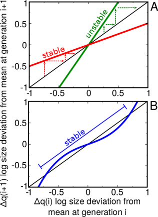
Figure 3: Conditions for stability of the deterministic part of cell-size control. A: Under linear control with negligible noise, $\Delta q(i+1)=(1-\lambda)\Delta q$. If $(1-\lambda)>1$ (green line) the system is unstable, while if $(1-\lambda)<1$ (red line) the system is stable. The black line reprents the marginally stable case $\Delta q(i+1)=\Delta q$. By using a similar argument (see Appendix A3), it is possible to show that if $|g(\Delta q)|<|\Delta q|$ for any $|\Delta q|$, then the system is globally stable. B: In the more general case of a locally stable point the basin of attraction can be obtained as the set of values of $\Delta q$ such that $|g(\Delta q)|<|\Delta q|$.

III.3 Inequalities defining the relevant parameters given a set of experimental observations.

This section derives general constraints on the relevant parameters given the number of observations through simple quantitative estimates. The above calculations unequivocally define $\lambda$ as the most important parameter at play, together with another scale defining the width of the noise. A further question is whether this is effectively the only relevant parameter. In order to answer this question, one has to consider higher order terms in the expansion, and ask when those terms play a role, and whether they can be identified from data. In fact, the number of available observations define whether a truncated expansion description is useful to describe the data.

The expansion around $\langle x_{0}\rangle$ (Eq. (11)) is effective as long as the fluctuations of size are sufficiently small. In order to estimate precisely the regime where the approximation is valid, we include the second order in the expansion

$$q_{0}(i+1)=\bar{q}_{\alpha}+(1-\lambda)\left(q_{0}(i)-\bar{q}_{\alpha}\right)+\gamma\frac{\left(q_{0}(i)-\bar{q}_{\alpha}\right)^{2}}{2}+\sigma\xi\ ,$$ (14)

where $\gamma=g^{\prime\prime}(0)$, the second derivative of the control function.

We set out to evaluate the difference between this process and the one defined by Eq. (12). The quadratic term is measurable from stochastic trajectories if it is sufficiently large compared to stochastic fluctuations. Thus, we evaluate the distribution of $q_{0}(i+1)-\bar{q}_{\alpha}-(1-\lambda)\left(q_{0}(i)-\bar{q}_{\alpha}\right)$ and ask weather, for given sample size and value of $q_{0}(i)$, its mean is significantly different from zero or not.

The error on the mean is given by the standard deviation divided by the square root of the sample size. Hence, the quadratic term is detectable if

$$\frac{\sigma}{\sqrt{T(q)}}<\gamma\frac{\left(q_{0}(i)-\bar{q}_{\alpha}\right)^{2}}{2}\ ,$$ (15)

where $T(q)$ is the number of cells with initial size $q$. Since the distribution of $q$ is approximately Gaussian (in the limit of $\gamma\approx 0$), the number of cells with initial size in a bin of width $\Delta q$ around $q$ is estimated by

$$T(q)=N\frac{\exp\left(-\frac{(q-\bar{q}_{\alpha})^{2}}{2\sigma_{q}^{2}}\right)}{\sqrt{2\pi\sigma_{q}^{2}}}\Delta q\ ,$$ (16)

where $N$ is the total number of cells. The bin size must be smaller than the standard deviation of the distribution, and we can parameterize it by defining $\Delta q=\epsilon\sigma_{q}$. The constraint on the total number of cells measured in order to recognize higher-order terms then reads

$$N>\frac{\sqrt{2\pi}\sigma_{q}}{\epsilon\sigma_{q}}\frac{\sigma^{2}}{\gamma^{2}}\frac{4}{(q-\bar{q}_{\alpha})^{4}}\exp\left(\frac{(q-\bar{q}_{\alpha})^{2}}{2\sigma_{q}^{2}}\right)\ .$$ (17)

The above expression reveals an important tradeoff (illustrated in Fig 4A). Choosing a value of $q$ close to the mean for the bin will give a large sample size in data, but also causes the effect to be measured to be very small, and increasingly close to the experimental resolution. Conversely, choosing a value of $q$ very far from the mean corresponds to larger effects, but needs large sample sizes to be measured. The optimal choice of $q$ to evaluate deviations from the linear model in the data is the one that minimizes the left side of the Eq (17). We have therefore

$$\begin{split}N>&\frac{1}{\epsilon}\frac{1}{\sigma_{q}^{2}\gamma^{2}}\lambda(2-\lambda)\min_{t}\frac{4\sqrt{2\pi}}{t^{4}}\exp\left(\frac{t^{2}}{2}\right)\\ &\approx\frac{4.6}{\epsilon}\lambda(2-\lambda)\frac{1}{\gamma^{2}\sigma_{q}^{2}}=\frac{4.6}{\epsilon}\lambda(2-\lambda)\frac{1}{\gamma^{2}\log\left(1+\operatorname{cv}_{x}^{2}\right)}\ .\end{split}$$ (18)

Where $\operatorname{cv}_{x}$ is the coefficient of variation of the distribution of $x$. In the available data, this is around $0.15$ Kennard2016 ; Taheri-Araghi2015 . Considering $\epsilon=0.1$ and, assuming $\lambda(2-\lambda)$ to be a number of order $1$ (which should be the case if $\lambda\approx 1/2$), we obtain $N\approx 1.5\cdot 10^{3}/\gamma^{2}$. The factor $\gamma^{2}$, which is set by the second derivative of $g(\cdot)$, plays a very important role here as its value sets the scale at which specific mechanisms can be distinguished.

IV Interpretability of mechanisms of division control.

This section relates the perturbative expansion and its interpretation to mechanisms of division control discussed in the literature, given the available data. We specifically consider the case of the constant added size model, proposed as a mechanism of division control across different conditions, obtaining the parameters of its expansion.

IV.1 The “concerted control” mechanism

Eq. (12) provides a generic description of division control for small fluctuations. When it is interpreted in terms of mechanisms of control, it corresponds to the simplest “concerted control” model, i.e. to a mix of sizer and timer behavior (as in the framework of ref.Amir2014 ). Specifically, since the time between divisions is $(q_{f}-q_{0})/\alpha$, setting $\tau=\tau_{0}+\xi$, where $\xi$ are Gaussian, independent, zero-mean random variables, one obtains

$$\tau_{0}=(1-\lambda)\frac{\log 2}{\alpha}+\frac{\lambda}{\alpha}\log\frac{x^{\ast}_{\alpha}}{x_{0}}\ .$$ (19)

The above equation can be interpreted as implementing the the control on cell division as a mixture of timer and sizer behavior Amir2014 . Indeed, the doubling time is set by a convex combination with mixing parameter $\lambda$ of a fixed time (set by the inverse mean growth rate $1/\alpha$) and a perfect sizer (set by a limit threshold size $x^{\ast}$ for cell division). A pure sizer model, recovered for $\lambda=1$ would set this conditional interdivision time as $\tau_{0}=\frac{\lambda}{\alpha}\log\frac{x^{*}_{\alpha}}{x_{0}}$, while a pure timer model ($\lambda=0$) defines $\tau_{0}$ as $\log 2/\alpha$. It is straightforward to show that, in the small noise limit, $x^{\ast}_{\alpha}=2\langle x_{0}\rangle=\langle x_{f}\rangle$. The concerted control is a consequence of the combination of these two decision processes, set by the parameter $\lambda$. As shown in section III.2 this process leads to stationary distributions of sizes if $0<\lambda<2$. Our previous calculations show that such an effective cell-cycle model (equivalent to the approach introduced in ref. Amir2014 ) can be characterized as the auto-regressive model giving a discrete-time Langevin equation with harmonic potential. As discussed above, this has a number of consequences, including a strict relation between the noise in $\tau$ and in $\log x_{0}$, and the fact that the characteristic times (in generations) for damping of fluctuations and perturbations (fluctuation-dissipation theorem) is $1/\lambda$.

As shown in section III.2 and previously suggested Amir2014 , the linear dependency of $\tau_{0}$ on $\log x_{0}$ can be seen as a first-order approximation of a generic function relating the doubling time to the initial size. Thus, nearly all models where one of the two terms in Eq. (19) is not strictly null are expected to behave similarly to this concerted control model as long as the probed initial cell sizes $x_{0}$ are close to their mean $\langle x_{0}\rangle_{\alpha}$, or equivalently as long as the noise in $\alpha\tau$ is small.

IV.2 The constant added size mechanism

We now consider the constant added size mechanism, written as a discrete Langevin dynamics on the logarithmic initial size $q$. The deterministic part is defined by

$$g\left(q-\bar{q}_{\alpha}\right)=q-\bar{q}_{\alpha}+\int dz\ F\left(z\right)\log\left(\frac{c+ze^{\bar{q}_{\alpha}-q_{0}}}{2}\right)\ ,$$ (20)

where $c$ is determined by imposing $g(0)=0$ and $F(\cdot)$ is the probability distribution of the relative fluctuations of the added size around its mean (Appendix A5). Expansion of this function gives $\lambda=1/2$, consistently with previous results Amir2014 , which guarantees stationarity of the process. The second-order term gives $\gamma=1/4$. Since all the parameters are fixed one can write Eq. (17), for the “adder” model as

$$N>\frac{55}{\epsilon}\frac{1}{\log\left(1+\operatorname{cv}^{2}_{x}\right)}\ .$$ (21)

Realistic values of $\operatorname{cv}_{x}$ are around $0.15$ Taheri-Araghi2015 . The remaining parameter $\epsilon$ defines how coarse is the binning. Since it must be by definition a small number (if it was not one would have to consider other sources of errors) we shall assume $\epsilon=0.1$. In this case we would obtain that at least $N\approx 50000$ cell divisions are required to distinguish between the adder model and any other model with the same first-order expansion.

This estimate sets therefore a threshold on the number of cells that one need to measure to have enough statistical power to observe non-linearity in the size control function $g(\Delta q)$. Fig. 4 compare the current available datasets with the estimated threshold, showing that all of them are below the estimated threshold. A linearization of $g(\Delta q)$ should be, for most available experimental data sets, sufficient to describe the main observations.

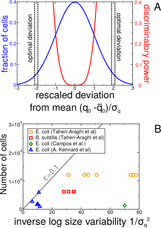
Figure 4: Estimated threshold of detectability of non-linear contributions to cell-division control. A: The trade-off between two competitive terms determines an optimal cell-size fluctuation to identify cell size control. One one hand, large deviations of size from the average, correspond to stronger corrections make differences between mechanism more detectable. On the other hand, fewer cells have large fluctuations, reducing the statistical power and increasing the sampling noise. The optimal fluctuation value is the one that minimizes the error on the inferred cell-size control mechanism. Our calculations (Eq. (17) show that, when fluctuations are rescaled by the variance of the distribution, the optimal value is independent of the cell-size control mechanism, as shown in the plots of the contributions described by Eqs (15) (discriminatory power, green line) and (17) (sampling level, blue line). B: Estimated detection threshold for $\epsilon=0.1$ (gray line) and data points corresponding to the available datasets. All the available data sets lay below the threshold of detectability, suggesting that a linear model of division control is sufficient to describe these data.

To make the result on the estimated threshold for detectability more concrete, we consider explicitly the case of the adder mechanism and its distinguishibility from the linearized model (Eq (12)). By definition, the adder mechanism predicts that the conditional mean (and distribution) of the added size, given initial size, is independent on initial size. While the first-order expansion of the framework defined here with $\lambda=1/2$ (and analogously for the model in ref. Amir2014 ) does not follow this functional trend (i.e., the next orders in the expansion are different), it shows a very small difference with the adder model in the empirical range of sizes, which might not be discerned with the sampling of available empirical data.

In order to further support this point, we employed direct numerical simulations at different number of realizations (mimicking experimental sampling levels). As explained above, the most complete information on the process is the transition probability $p(x_{f}|x_{0},\alpha)$. For an adder, this probability depends only on the difference $x_{f}-x_{0}$, i.e. $p(x_{f}-x_{0}|x_{0})$ is independent of $x_{0}$, or, in other words, the conditional distribution of added size given initial size does not depend on the initial size. The fact that $p(x_{f}-x_{0}|x_{0})$, obtained for different $x_{0}$, collapses has been interpreted in ref. Taheri-Araghi2015 as evidence in favor of the adder mechanism of division control. To gain more insight into this conclusion, we simulated the first-order process (Eq. (14)) with $\lambda=1/2$. Fig. 5, reports the binned histograms of rescaled added sizes for cells with different intial sizes, and using similar bin sizes as in ref. Taheri-Araghi2015 , the very good collapse shows that the difference between the probability distributions is barely detectable at the available level of sampling.

We quantified the error on the collapse measuring the average $L_{2}$ distance between all the pairs of curves plotted in Fig. 5A. This error, measured for different values of $\lambda$ and different sample sizes, can be compared with the expected error due to fluctuations in the adder, also estimated as the avarage $L_{2}$ distance between distribution of the added size given the initial one. As expected, Fig. 5A shows that the error is minimal when $\lambda=0.5$. Interestingly, the measured error does not depend on the sample size, while the expected error from the adder model decreases as the number of measured cells increases. Fig. 5B shows that the two error measures become comparable when $N$ is between $10000$ and $20000$, which is around the same order of magnitude of the number of cells measured in ref. Taheri-Araghi2015 . Thus, the test presented in Fig. 5 might work with the existing sampling levels.

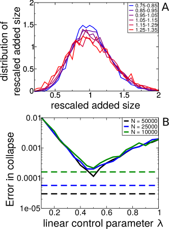
Figure 5: Detectability of adder mechanism from simulated models and direct test. Plotted data refer to simulations of an models with realistic parameters and sampling of cells. A: Conditional distribution of added size fiven intial size for different initial sizes (different colors) obtained with the linearized model (Eq. (14)) with $\lambda=0.5$. The linearized model reproduces visually the collapse expected for the adder model. The simulations consider conservatively a coefficient of variation of the added size equal to $0.3$ (which is larger than the observed values Taheri-Araghi2015 ) and a total number of cells $N=50000$. B: Error test on the collapse of the distribution of added size (estimated as the average $L_{2}$ distance between all pairs of curves) for different values of $N$ and $\lambda$. The horizontal dashed lines represent the expected error in collapse in the adder model due to fluctuations. For these parameter values, the error in the collapse for the model with $\lambda=0.5$ starts to be relevant when $N\sim 10000$. This test may be applied to empirical data: in order for an adder to be detectable, the solid line should stay above the dashed line.

V Discussion

Our approach provides a map between an autoregressive discrete-time formalism of cell division control and a continuous-time description based on hazard-rate functions, showing the impact on both formalisms of the observed scaling behavior of cell sizes and doubling times. This map connects the approaches used in refs Osella2014a ; Jun2015 ; Kennard2016 with those of refs. Amir2014 ; Campos2014 ; Soifer2016 , and leads us to propose a unified framework (with discrete-time Langevin equations) embracing both formalisms to develop and explore effective models of cell division. The framework has the additional advantage of showing how parameter-poor models describing different kinds of cell division control are possible for multiple mechanisms.

The use of a discrete-time Langevin formalism for the logarithmic size leads to a the simple physical analogy with a fluctuationg system and guides in the interpretation of the model parameters. The same formalism also enables the applicability of familiar concepts in the statistical physics of fluctuating systems, such as correlation, response, and fluctuation-dissipation relations. We anticipate that such concepts will become useful for future studies of dividing cells in fluctuating environments. An important extension of the present framework should incorporate growth fluctuations. Recent studies Harris2016 ; Iyer-Biswas2014 show clear indications that the assumption of constant growth rate $\alpha$ is an oversimplification, and that size homeostasis needs to be understood by addressing contributions from both growth and cell division. Possibly the most relevant result from recent experimental work is the existence of a mechanism governed by a single size scale. The “microscopic” origin of this length scale is a relevant question that is not solved by any of the mechanisms proposed in the literature.

By exploring systematically a perturbative expansion of the model, we show how the unified framework defined here can lead to similar equations to the ones introduced in ref. Amir2014 , with the advantage of elucidating the direct link with the hazard rate function. The main difference is found in the dependence of the noise term on the growth rate $\alpha$. In the setting defined here, there is no dependency, while ref. Amir2014 assumes a dependency (see Sec. IV). The importance of this difference is that in the setting defined here the distributions of division times collapse as observed experimentally. Furthermore, the more general framework presented here can be used to compute the next orders of the expansions, and to study hierarchically the mechanisms leading to homeostasis.

The perturbative approach also leads to relevant insight on the ability to distinguish different control mechanisms from data. Overall, our results indicate that a linearization of the control function $g(\Delta q)$ should be, for most currently available experimental data sets, sufficient to describe the main observations. Thus, for most practical purposes, the physical analogy with the discrete-time version of harmonic fluctuations for logarithmic size is valid. The bounds on sampling levels that we derive analytically estimate the number of cell divisions that need to be measured in order to evaluate higher-order nonlinear “anharmonic” terms, which are necessary to pinpoint precise mechanisms.

Importantly, these calculations show that there is an optimal choice of cell sizes to test the deviations. On the one hand, testing sizes that deviate a great deal from the average will show stronger corrections, and make differences between mechanism more detectable. On the other hand, fewer cells have large fluctuations, reducing the statistical power and increasing the sampling noise of such measurements. The optimal fluctuation value is the one that minimizes the error on the inferred cell-size control mechanism. Importantly, the calculations show that, when fluctuations are rescaled by the variance of the distribution, the optimal value is independent of the cell-size control mechanism. Thus, we expect that different division control functions should be distinguishable without requiring an ad hoc number of observations.

Comparing the detection threshold with the number of observations made in available studies, we find that the number of measured cells should typically be insufficient to draw any strong conclusions beyond the linear approximation. By applying our methods, we show that at the current sampling levels, it might be very hard to distinguish it from linear response (compatible with many scenarios), even with sophisticated tests such as collapse of the conditional distribution of added size. This poses important caveats on the possibility of determining a specific mechanism from specific data sets and in the interpretation of measured trends as “microscopic” mechanisms of size control.

We propose the method developed in Fig. 5B as an effective way, applicable to empirical data, to test for deviations from the behavior of the linearized model, which should work with sampling levels that can be attained experimentally with existing approaches. We are currently working on extending this approach using Bayesian statistics and producing reliable statistical estimators of the relevant parameters ($\lambda$ and $\gamma$) of the division control function.

VI Acknowledgements

This work was supported by the International Human Frontier Science Program Organization, grant RGY0070/2014.

Supplementary Appendix

A1 Collapse of the initial size and doubling time distributions

This section discusses the implications of the observed collapse of doubling time and initial size distributions on the division rate function $h_{d}$.

The initial size distribution $p_{b}^{\ast}(x_{0}|\alpha)$ in a given condition characterized by mean growth rate $\alpha$, is given by

$$p_{b}^{\ast}(x_{0}|\alpha)=2\int_{0}^{+\infty}\mathrm{d}x_{0}^{\prime}\ \theta(2x_{0}-x_{0}^{\prime})p_{b}^{\ast}(x_{0}^{\prime}|\alpha)p(2x_{0}|x_{0}^{\prime},\alpha)\ ,$$ (A1)

where $\theta(\cdot)$ is the Heaviside function.

The collapse of initial sizes implies that $p_{b}^{\ast}(y|\alpha)=p_{b}^{\ast}(y)$ is independent of $\alpha$, with $y=x_{0}/\langle x_{0}\rangle_{\alpha}$. Imposing this condition in Eq (A1) implies that

$$p_{b}^{\ast}(y)=2\int_{0}^{\infty}\mathrm{d}y^{\prime}\ \theta(2y-y^{\prime})p_{b}^{\ast}(y^{\prime})p(2y|y^{\prime},\alpha)\ .$$ (A2)

This equation immediately shows that a necessary and sufficient condition for the collapse is that the conditioned distribution does not depend on $\alpha$, i.e.,

$$p(y_{f}|y_{0},\alpha)=\tilde{p}(y_{f}|y_{0})\ .$$ (A3)

The division rate function $h_{d}(x,x_{0})$ is related to the above conditioned distribution by the following equation

$$\begin{split}h_{d}(x,x_{0},\alpha)=&-\log\int_{x_{0}}^{x}\mathrm{d}z\ p(z|x_{0},\alpha)=\\ =&-\log\int_{x_{0}/\langle x_{0}\rangle_{\alpha}}^{x/\langle x_{0}\rangle_{\alpha}}\mathrm{d}y\ \tilde{p}(y|x_{0}/\langle x_{0}\rangle_{\alpha})\ .\end{split}$$ (A4)

the collapse of initial size distributions is therefore equivalent to collapse of the division hazard rate when rescaled by mean initial sizes, i.e.

$$h_{d}(x,x_{0},\alpha)=\tilde{h}(\frac{x}{\langle x_{0}\rangle_{\alpha}},\frac{x_{0}}{\langle x_{0}\rangle_{\alpha}})$$ (A5)

We now consider the collapse of doubling-time distributions. The conditioned distribution for final sizes can be written as

$$p(x_{f}|x_{0},\alpha)=\tilde{p}(\frac{x_{f}}{\langle x_{0}\rangle_{\alpha}},\frac{x_{0}}{\langle x_{0}\rangle_{\alpha}})=\widehat{p}(\frac{x_{f}}{x_{0}},\frac{x_{0}}{\langle x_{0}\rangle_{\alpha}})\ .$$ (A6)

Since $\log(x_{f}/x_{0})=\alpha\tau$, the above expression, combined with Eq (A3), implies the following condition for the collapse of the distribution of doubling times

$$\alpha p_{t}^{\ast}(\tau|x_{0},\alpha)=\widehat{p}(\alpha\tau,\frac{x_{0}}{\langle x_{0}\rangle_{\alpha}})\ .$$ (A7)

The joint collapse of the distribution of doubling times and initial cell sizes impose conditions on size control. In other words, a control of cell division obeying to the condition described in Eq. (A3) and (A7) will generate universal size and doubling-time distribution.

In particular, a necessary condition for this to hold is that the product of the mean doubling time and the mean growth rate $\alpha\langle\tau\rangle_{\alpha}$, does not depend on the mean growth rate in a given condition $\alpha$.

A2 Full derivation of the mapping between discrete-time Langevin equation and division hazard rate.

This section shows in full generality the mapping between a discrete-time Langevin formalism and the corresponding division hazard rate.

The discrete equation for the logarithm of the initial size is

$$q(i+1)=\bar{q}_{\alpha}+g(q(i)-\bar{q}_{\alpha})+\eta(q(i)-\bar{q}_{\alpha})\ ,$$ (A8)

where

$$g(q_{0}-\bar{q}_{\alpha})=\int dq\ \rho(q|q_{0},\alpha)q-\bar{q}_{\alpha}-\log(2)\ ,$$ (A9)

while $\eta$ is a random variable with distribution $\rho(q-\bar{q}_{\alpha}-\log(2)-g(q_{0}-\bar{q}_{\alpha})|q_{0},\alpha)$.

Using Eq. (2) we can write

$$g(q_{0}-\bar{q}_{\alpha})=\int_{x^{\ast}e^{q_{0}}}^{\infty}dx\ p(x|x^{\ast}e^{q_{0}},\alpha)\log\left(\frac{x}{x^{\ast}}\right)-\bar{q}_{\alpha}-\log(2)\ ,$$ (A10)

and introducing Eq. (6) we obtain

$$\begin{split}g(q_{0}-\bar{q}_{\alpha})&=\int_{x^{\ast}e^{q_{0}}}^{\infty}dx\ \left(-\frac{d}{dx}\exp\left(\int_{x_{0}}^{x}ds\ h_{d}\left(s,x_{0},\alpha\right)\right)\right)\log\left(\frac{x}{x^{\ast}}\right)-\bar{q}_{\alpha}-\log(2)=\\ &=-\exp\left(\int_{x^{\ast}e^{q_{0}}}^{x}ds\ h_{d}\left(s,x_{0},\alpha\right)\log\left(\frac{x}{x^{\ast}}\right)\right)\Bigr{|}_{x=x^{\ast}e^{q_{0}}}^{\infty}+\int_{x^{\ast}e^{q_{0}}}^{\infty}dx\ \exp\left(\int_{x_{0}}^{x}ds\ h_{d}\left(s,x_{0},\alpha\right)\right)\frac{1}{x}-\bar{q}_{\alpha}-\log(2)\ ,\end{split}$$ (A11)

and the final expression reads

$$g(q_{0}-\bar{q}_{\alpha})=q_{0}-\bar{q}_{\alpha}+\int_{x^{\ast}e^{q_{0}}}^{\infty}\frac{dx}{x}\ \exp\left(\int_{x^{\ast}e^{q_{0}}}^{x}ds\ h_{d}\left(s,x^{\ast}e^{q_{0}},\alpha\right)\right)-\log(2)\ .$$ (A12)

The hazard rate function cannot be derived from Eq. (A8) without specifying the form of the noise $\eta(q(i)-\bar{q}_{\alpha})$. Assuming that the distribution of the noise is Gaussian, we obtain

$$\Delta q_{0}(i+1)=g\left(\Delta q_{0}(i)\right)+\sigma\left(\Delta q_{0}(i)\right)\xi\ ,$$ (A13)

where $\xi$ in this expression is an Gaussian random variable of zero mean and unit variance and $\sigma(\cdot)$ a proper function of $\Delta q_{0}(i)=q_{0}(i)-\bar{q}_{\alpha}$. The division probability at log-size $q$ given and initial log-size $q_{0}$ is therefore

$$\rho(q|q_{0},\alpha)=\frac{1}{\sqrt{2\pi}\sigma(q_{0}-\bar{q}_{\alpha})}\exp\left(-\frac{\left(q-\bar{q}_{\alpha}-g\left(q_{0}-\bar{q}_{\alpha}\right)\right)^{2}}{2\sigma(q_{0}-\bar{q}_{\alpha})^{2}}\right)\ ,$$ (A14)

using the fact that

$$\ h_{d}(x,x_{0},\alpha)=-\frac{d}{dx}\log P_{0}(x,x_{0},\alpha)\ ,$$

where

$$P_{0}(x,x_{0},\alpha)=\int_{x_{0}}^{x}dz\ p(z|x_{0},\alpha)\ ,$$

we obtain that

$$\begin{split}\ h_{d}(x,x_{0},\alpha)&=-\frac{d}{dx}\log\int_{x_{0}}^{x}dy\ p(y|x_{0},\alpha)=-\frac{dq}{dx}\frac{d}{dq}\log\int_{q_{0}}^{q}dp\ \rho(p|q_{0},\alpha)=\\ &-\frac{1}{x}\frac{d}{dq}\log\frac{1}{2}\left(1-\text{Erf}\left(\frac{q-\bar{q}_{\alpha}-g\left(q_{0}-\bar{q}_{\alpha}\right)}{\sqrt{2}\sigma(q_{0}-\bar{q}_{\alpha})}\right)\right)\Bigr{|}^{q=\log(x/x^{*})}_{q_{0}=\log(x_{0}/x^{*})}\ ,\end{split}$$ (A15)

where the error function Erf is defined as

$$\text{Erf}(x):=\frac{2}{\sqrt{\pi}}\int_{0}^{x}dt\ e^{-t^{2}}\ \ .$$

We finally obtain

$$h_{d}(x,x_{0},\alpha)=\frac{1}{x}\left(g_{\sigma}\left(\frac{q-\bar{q}_{\alpha}-g\left(q_{0}-\bar{q}_{\alpha}\right)}{\sqrt{2}\sigma(q_{0}-\bar{q}_{\alpha})}\right)\right)\Bigr{|}_{q=\log(x/x^{*})}^{q_{0}=\log(x_{0}/x^{*})}\ ,$$

where

$$g_{\sigma}(y)=\frac{1}{\sqrt{2\pi}\sigma}\frac{\exp(-y^{2})}{1-\text{Erf}(y)}\ .$$

In the next session we show the explicit calculation in the case of linear $g(\cdot)$ and constant $\sigma(\cdot)$.

A2.1 Division rate for linearized model

As explained in the main text, one can linearize Eq. (A8) around its equilibrium, obtaining

$$q_{0}(i+1)=\bar{q}_{\alpha}+(1-\lambda)\left(q_{0}(i)-\bar{q}_{\alpha}\right)+\sigma\xi\ .$$ (A16)

In this case Eq. (A2) reads

$$h_{d}(x,x_{0},\alpha)=\frac{1}{\alpha x}g_{\sigma}\left(\frac{1}{\sqrt{2}\sigma\alpha}\log\frac{x}{x_{0}^{(1-\lambda)}x^{\ast\lambda}}\right)\ .$$

A3 Conditions for stationarity

This section discusses under which conditions Eq. (10) admits a well defined stationary size distribution. The scaling of stationary distribution is the only assumption that we used to derive Eq. (10). Any division control must, by definition, regulate sizes and stabilize size fluctuations. A necessary condition is therefore that that the deterministic equation corresponding to Eq. (10) has a fixed point and that fixed point is (at least) locally asymptotically stable.

The fixed point of the deterministic part of Eq. (10) is a solution of the equation $q^{\ast}=\bar{q}_{\alpha}+g\left(q^{\ast}-\bar{q}_{\alpha}\right)$. This fixed point is asymptotically locally stable iff

$$\left|\left(\frac{dg}{dq}\Bigr{|}_{q=q^{\ast}}\right)\right|=|1-\lambda|<1\ .$$ (A17)

Since $\bar{q}_{\alpha}$ was define up to an arbitrary dimensionless constant $c$, we can always choose $q^{\ast}=\bar{q}_{\alpha}$ (i.e., $\bar{q}_{\alpha}$ is equal to $\langle\log x_{0}\rangle_{\alpha}$). We obtain therefore that $g(0)=0$ and $\lambda=1-g^{\prime}(0)$. This condition is necessary, but not sufficient to guarantee stationarity of the process.

More generally, the deterministic part of Eq. (10) implies that the equilibrium is unique and globally stable if and only if $|g(\Delta q)|<|\Delta q|$ for any $\Delta q$, where $\Delta q_{0}(i)=q_{0}(i)-\bar{q}_{\alpha}$. In particular, if the the function $g(\cdot)$ is monotonic and has only one fixed point which is locally stable, then that fixed point is globally stable. This property sets a minimal condition that division control has to fulfill to guaranty stationarity of cell size distribution. If the fixed point was not globally stable, than a large enough fluctuation would not be corrected by feedback control. When the stochasticity is taken into account, since the noise in Eq. (10) can be multiplicative, global stability does not guarantee stationarity of the size distribution in general. On the other hand, the requirement of having a stationary distribution is not necessarily biologically relevant and is not needed to have homeostasis. The basin of attraction of the fixed point $\Delta q=0$, is determined by the values of $\Delta q$ such that $|g(\Delta q)|<|\Delta q|$. What is relevant for homeostasis is that the basin of attraction determined by $g(\dot{)}$ is large enough compared to the typical fluctuations. This would guarantee that most of the cells are able to control fluctuation of their size, and loss of control is a rare event.

To characterize the effect of multiplicative noise on the existence of a stationary size distribution, we study a general expansion of $\sigma\left(\Delta q_{0}(i)\right)$ in Eq. (11)

$$\Delta q_{0}(i+1)=(1-\lambda)\Delta q_{0}(i)+\left(\sigma+\beta\Delta q_{0}(i)\right)\xi\ ,$$ (A18)

where $\beta=\sigma^{\prime}(0)$. If $\beta=0$, then this process guarantees homeostasis for any $|1-\lambda|<1$. In the case $\beta\neq 0$, one can write recursive equations for the moments of the distribution of sizes, given an arbitrary initial condition. The equation for the mean corresponds, obviously, to the deterministic equation. The recursive equation for the variance reads

$$\begin{split}&\langle\Delta q_{0}(i+1)^{2}\rangle=\\ &(1-\lambda)^{2}\langle\Delta q_{0}(i)^{2}\rangle+\sigma^{2}+\beta^{2}\langle\Delta q_{0}(i)^{2}\rangle+2\sigma\beta\langle\Delta q_{0}(i)\rangle\ .\end{split}$$ (A19)

Starting from a deterministic initial condition $\Delta q_{0}(0)$, using the result of Eq. (13) and solving the recursive equation one can obtain the time evolution of the variance. In the case of $\Delta q_{0}(0)=0$ it reads

$$\langle\left(q_{0}(n)-\bar{q}_{\alpha}\right)^{2}\rangle=\sigma\frac{1-\left((1-\lambda)^{2}+\beta^{2}\right)^{n}}{\lambda(2-\lambda)-\beta^{2}}\ .$$ (A20)

It is simple to see that the variance converges to a constant if and only if $(1-\lambda)^{2}+\beta^{2}<1$, i.e., $\beta^{2}<\lambda(2-\lambda)$. In case of multiplicative noise, the stationarity of the size distribution depends, in a non trivial concerted way, from both the strength of control and the magnitude of the noise.

A4 Solution of the linearized model

In this section we discuss the solution of the linearized model defined by the discrete Langevin equation

$$\Delta q_{0}(i+1)=(1-\lambda)\Delta q_{0}(i)+\sigma\xi\ .$$ (A21)

This equation defines the distribution of initial size at generation $i+1$ given the one of generation $i$, as

$$\rho^{i+1}(\Delta q)=\int_{-\infty}^{\infty}d\Delta q^{\prime}\ \rho^{i}(\Delta q^{\prime})\varrho\left(\frac{\Delta q-(1-\lambda)\Delta q^{\prime}}{\sigma}\right)\ ,$$ (A22)

where $\varrho(\cdot)$ is a Gaussian distribution with zero mean and unit variance. One can iterate this equation, and, exploiting the fact that the Gaussian is stable under convolution, one obtains

$$\begin{split}\rho^{i+1}(\Delta q)=\\ =\int_{-\infty}^{\infty}d\Delta q^{\prime}\ \rho^{0}(\Delta q^{\prime})\varrho\left(\frac{\Delta q-\langle\Delta q(i)\rangle_{\Delta q^{\prime}}}{\sqrt{\langle\Delta q(i)^{2}\rangle_{\Delta q^{\prime}}-\langle\Delta q(i)\rangle^{2}_{\Delta q^{\prime}}}}\right)\ ,\end{split}$$ (A23)

where $\langle\Delta q_{0}(i)\rangle_{\Delta q^{\prime}}$ is the average of $\Delta q$ at generation $i$ given that the initial log-size displacement at the first generation $i=0$ was $\Delta q^{\prime}$. In order to have an explicit equation, we need just to calculate the $\langle\Delta q_{0}(i)\rangle_{\Delta q(0)}$ and $\langle\Delta q_{0}(i)^{2}\rangle_{\Delta q(0)}$.

The mean displacement can be calculated, by solving

$$\langle\Delta q_{0}(i+1)\rangle_{\Delta q(0)}=(1-\lambda)\langle\Delta q_{0}(i+1)\rangle_{\Delta q(0)}+\sigma\xi\ .$$ (A24)

with initial condition $\Delta q_{0}(0)$. The solution reads

$$\langle\Delta q_{0}(n)\rangle_{\Delta q(0)}=\Delta q(0)(1-\lambda)^{n}\ .$$ (A25)

A similar equation can be written for the second moment

$$\langle\Delta q_{0}(i+1)^{2}\rangle_{\Delta q(0)}=(1-\lambda)^{2}\langle\Delta q_{0}(i)^{2}\rangle_{\Delta q(0)}+\sigma^{2}\ ,$$ (A26)

whose solution is

$$\langle\Delta q_{0}(n)^{2}\rangle_{\Delta q(0)}=\sigma^{2}\frac{1-(1-\lambda)^{2n}}{\lambda(2-\lambda)}+(1-\lambda)^{2(n-1)}\Delta q(0)^{2}\ .$$ (A27)

Therefore we finally obtain

$$\langle\Delta q_{0}(n)^{2}\rangle_{\Delta q(0)}-\langle\Delta q_{0}(n)\rangle^{2}_{\Delta q(0)}=\sigma^{2}\frac{1-(1-\lambda)^{2n}}{\lambda(2-\lambda)}+(1-\lambda)^{2n}\frac{\lambda(2-\lambda)}{(1-\lambda)^{2}}\Delta q(0)^{2}\ .$$ (A28)

By taking the limit $n\to\infty$ of Eq. (A27) we obtain the stationary variance, which reads

$$\sigma_{q}^{2}=\frac{\sigma^{2}}{\lambda(2-\lambda)}\ .$$ (A29)

The stationary distribution is therefore

$$\rho^{\ast}_{b}(q)=\frac{1}{\sqrt{2\pi\sigma_{q}^{2}}}\exp\left(-\frac{(q-\bar{q}_{\alpha})^{2}}{2\sigma_{q}^{2}}\right)\ ,$$ (A30)

and therefore the one of the sizes at birth is

$$p_{b}^{\ast}(x_{0})=\frac{1}{\sqrt{2\pi\sigma_{q}^{2}}x_{0}}\exp\left(-\frac{(\log(x_{0}/x^{\ast})-\bar{q}_{\alpha})^{2}}{2\sigma_{q}^{2}}\right)\ ,$$ (A31)

which has mean

$$\langle x_{0}\rangle_{\alpha}=x^{\ast}e^{\bar{q}_{\alpha}+\sigma^{2}_{q}/2}\ ,$$ (A32)

and variance

$$\sigma^{2}_{x_{0}}=(x^{\ast})^{2}e^{2\bar{q}_{\alpha}}\left(e^{\sigma^{2}_{q}}-1\right)e^{\sigma^{2}_{q}}\ .$$ (A33)

The coefficient of variation of the size at birth is defined as

$$\frac{\sigma^{2}_{x_{0}}}{\langle x_{0}\rangle_{\alpha}^{2}}=\left(e^{\sigma^{2}_{q}}-1\right)\ ,$$ (A34)

and therefore we have

$$\sigma^{2}_{q}=\log\left(1+\left(\frac{\sigma_{x_{0}}}{\langle x_{0}\rangle_{\alpha}}\right)^{2}\right)\ .$$ (A35)

A5 Perturbative expansion and identification of parameters for the adder model

An adder mechanism of division control corresponds to a division probability of the form

$$p(x_{f}|x_{0},\alpha)=F_{\alpha}(x_{f}-x_{0})\ .$$ (A36)

Using the scaling of the stationary distributions of equation (A6), we obtain

$$F_{\alpha}(x_{f}-x_{0})=p(x_{f}|x_{0},\alpha)=\frac{1}{\langle x_{0}\rangle_{\alpha}}F\left(\frac{x_{f}-x_{0}}{\langle x_{0}\rangle_{\alpha}}\right)\ .$$ (A37)

This equation is consistent with the collapse of the probabilities of added size as observed in ref. [4].

By using Eq. (A9) and introducing $q=\log(x/x^{*})$, one obtains the functional form of $g(\cdot)$

$$g(q_{0}-\bar{q}_{\alpha})=\int dx\ p(x|x^{*}e^{q}_{0},\alpha)\log(x/x^{*})-\bar{q}_{\alpha}-\log(2)\ ,$$ (A38)

and, by introducing the scaling of Eq. (A37), this expression reads

$$\begin{split}g(q_{0}-\bar{q}_{\alpha})&=\frac{1}{\langle x_{0}\rangle_{\alpha}}\int dx\ F\left(\frac{x-x^{*}e^{q_{0}}}{\langle x_{0}\rangle_{\alpha}}\right)\log(x/x^{*})-\bar{q}_{\alpha}-\log(2)=\\ &=ce^{-\bar{q}_{\alpha}}\int dxF\left(\frac{x}{\langle x_{0}\rangle_{\alpha}}-ce^{q_{0}-\bar{q}_{\alpha}}\right)\log(x/x^{*})-\bar{q}_{\alpha}-\log(2)=\\ &=\int ds\ F\left(s-ce^{q_{0}-\bar{q}_{\alpha}}\right)\log(s)-\log(2)=\\ &=\int dz\ F\left(z\right)\log\left(z+ce^{q_{0}-\bar{q}_{\alpha}}\right)-\log(2)\ ,\end{split}$$ (A39)

leading to the final expression,

$$\begin{split}g(q_{0}-\bar{q}_{\alpha})&=q_{0}-\bar{q}_{\alpha}+\int dz\ F\left(z\right)\log\left(\frac{c+ze^{\bar{q}_{\alpha}-q_{0}}}{2}\right)\ ,\end{split}$$ (A40)

where $c$ is an arbitrary constant entering the definition of $\bar{q}_{\alpha}=\log(c\langle x_{0}\rangle_{\alpha}/x^{*})$. As explained in the main text, we fix the value of that constant to have $g(0)=0$. Under this choice, $c$ is defined as the solution of

$$\int dz\ F\left(z\right)\log\left(\frac{c+z}{2}\right)=0\ .$$ (A41)

In a similar way, the value of the control parameter $\lambda$ can be obtained from the following equation

$$\begin{split}\lambda=1-g^{\prime}(0)=\int dz\ F\left(z\right)\frac{z}{c+z}\ .\end{split}$$ (A42)

Since the value of $\lambda$ appears as first order in an expansion around the mean initial logarithmic cell size, we can neglect size fluctuations in calculating its value, since they correspond to sub-leading terms. Note, however, that these sub-leading terms have to be considered when other terms than the first order are included in the expansion. Since in the adder model $\langle x_{f}-x_{0}\rangle=\langle x_{0}\rangle$, we have (up to sub-leading terms) from Eq. (A37)

$$\begin{split}\langle z\rangle=\int dz\ F\left(z\right)z=1\ .\end{split}$$ (A43)

Therefore, by neglecting fluctuations in Eq. (A41), i.e. by imposing $F\left(z\right)=\delta(z-1)$, we obtain $c=1$ and therefore $\lambda=1/2$. In case we are also considering quadratic term in the expansion of $g(\dot{)}$, we should include also a correction on this value, by a factor that depends on the variance of the added size.

In the following we consider an explicit case of the adder model. We assume that $p(x_{f}|x_{0},\alpha)$ is a lognormal distribution, which correspond to

$$F(z)=\frac{1}{\sqrt{2\pi}z\sigma_{a}}\exp\left(-\frac{(\log z)^{2}}{2\sigma_{a}^{2}}\right)\ .$$ (A44)

We have therefore $\langle z\rangle=\exp(\sigma_{a}^{2}/2)$ and

$$\langle z^{2}\rangle-\langle z\rangle^{2}=e^{2\sigma_{a}^{2}}-e^{\sigma_{a}^{2}}$$

By introducing this expression in Eq. (A40) we obtain

$$\begin{split}g(q)&=q+\int dz\ \frac{1}{\sqrt{2\pi}z\sigma_{a}}\exp\left(-\frac{(\log z)^{2}}{2\sigma_{a}^{2}}\right)\log\left(\frac{c+ze^{-q}}{2}\right)\ .\end{split}$$ (A45)

By expanding this expression up to second order in $q$, we obtain

$$\begin{split}g(q)&\approx q\left\langle\frac{c}{c+z}\right\rangle+\frac{q^{2}}{2}\left\langle\frac{cz}{(c+z)^{2}}\right\rangle\ .\end{split}$$ (A46)

Assuming that the fluctuations are small, it is natural to expand the terms in $z$ around $z=\langle z\rangle$. Eq. (A41) then reduces to

$$\begin{split}0=\left\langle\log\frac{c+z}{2}\right\rangle\\ \approx\log\frac{c+\langle z\rangle}{2}+\frac{\left\langle(z-\langle z\rangle)^{2}\right\rangle}{2(c+\langle z\rangle))^{2}}\\ \approx\log\frac{c+1}{2}+\frac{\sigma_{z}^{2}}{2(1+c)}\ ,\end{split}$$ (A47)

and therefore

$$\begin{split}c\approx 1-\frac{\sigma_{z}^{2}}{4}\ .\end{split}$$ (A48)

Expanding Eq. (A46) around $\langle z\rangle$, and introducing the explicit dependence on $\sigma_{z}$, we obtain

$$\begin{split}g(q)&\approx q\left(\frac{1}{2}-\frac{\sigma_{z}^{2}}{16}+o(\sigma_{z}^{4})\right)+\frac{q^{2}}{2}\left(\frac{1}{4}+o(\sigma_{z}^{2})\right)\ ,\end{split}$$ (A49)

which corresponds to $\lambda=1/2+\sigma_{z}^{2}/16$.

In a similar way, it is possible to estimate the variance of the noise term in the discrete Langevin formalism

$$\begin{split}&\sigma(q_{0}-\bar{q}_{\alpha})^{2}=\\ &\int dx\ p(x|x^{*}e^{q}_{0},\alpha)\left(\log(x/x^{*})-\bar{q}_{\alpha}-\log(2)\right)^{2}-g(q_{0}-\bar{q}_{\alpha})^{2}\ ,\end{split}$$ (A50)

and, by substituting for $F(z)$ in this expression,

$$\begin{split}\sigma(q)^{2}=\int dx\ F(z)\left(q+\log\left(\frac{c+ze^{-q}}{2}\right)\right)^{2}-g(q_{0}-\bar{q}_{\alpha})^{2}\ .\end{split}$$ (A51)

By expanding it up to the first order, on obtains

$$\begin{split}\sigma(q)^{2}\approx\left\langle\left(\log\left(\frac{c+z}{2}\right)\right)^{2}\right\rangle+q\left\langle\frac{2c\log\left(\frac{c+z}{2}\right)}{c+z}\right\rangle\ .\end{split}$$ (A52)

We can calculate explicitly the two terms in the case of a Lognormal $F(z)$ in the limit of small $\sigma_{z}$, and we obtain

$$\begin{split}\sigma(q)^{2}\approx\frac{\sigma_{z}^{2}}{4}-\frac{\sigma_{z}^{2}}{4}q\ .\end{split}$$ (A53)

and finally

$$\begin{split}\sigma(q)\approx\frac{\sigma_{z}}{2}-\frac{\sigma_{z}}{4}q\ .\end{split}$$ (A54)

In general, a Lognormal distribution does not result from a discrete-time Langevin process with a normal noise as in Eq. (11). On the other hand, since we are expanding for small fluctuations, the errors made approximating it with a normal noise are sub-leading. Using the notation

$$\begin{split}\Delta q(i+1)=(1-\lambda)\Delta q(i)+\gamma\frac{\left(\Delta q(i)\right)^{2}}{2}+\left(\sigma+\beta\Delta q(i)\right)\xi\ ,\end{split}$$ (A55)

we have that, for the adder model

$$\begin{split}&\lambda=\frac{1}{2}+\frac{\sigma_{z}^{2}}{16}+o(\sigma_{z}^{3})\\ &\gamma=\frac{1}{4}-\frac{\sigma_{z}^{2}}{16}+o(\sigma_{z}^{3})\\ &\sigma=\frac{\sigma_{z}}{2}+o(\sigma_{z}^{2})\\ &\beta=-\frac{\sigma_{z}}{2}+o(\sigma_{z}^{2})\ .\end{split}$$ (A56)

References

- [1] Andrew S. Kennard, Matteo Osella, Avelino Javer, Jacopo Grilli, Philippe Nghe, Sander J Tans, Pietro Cicuta, and Marco Cosentino Lagomarsino. Individuality and universality in the growth-division laws of single E. coli cells. Physical Review E, 93(1):012408, jan 2016.
- [2] Srividya Iyer-Biswas, Charles S Wright, Jonathan T Henry, Klevin Lo, Stanislav Burov, Yihan Lin, Gavin E Crooks, Sean Crosson, Aaron R Dinner, and Norbert F Scherer. Scaling laws governing stochastic growth and division of single bacterial cells. Proceedings of the National Academy of Sciences of the United States of America, 111(45):15912–7, dec 2014.
- [3] Andrea Giometto, Florian Altermatt, Francesco Carrara, Amos Maritan, and Andrea Rinaldo. Scaling body size fluctuations. Proc. Natl. Acad. Sci. (U.S.A.), 110(12):4646–50, Mar 2013.
- [4] Sattar Taheri-Araghi, Serena Bradde, John T Sauls, Norbert S Hill, Petra Anne Levin, Johan Paulsson, Massimo Vergassola, and Suckjoon Jun. Cell-size control and homeostasis in bacteria. Current biology : CB, 25(3):385–91, mar 2015.
- [5] Ariel Amir. Cell Size Regulation in Bacteria. Physical Review Letters, 112(20):208102, may 2014.
- [6] Matteo Osella, Eileen Nugent, and Marco Cosentino Lagomarsino. Concerted control of Escherichia coli cell division. Proceedings of the National Academy of Sciences of the United States of America, 111(9):3431–5, mar 2014.
- [7] Manuel Campos, Ivan V Surovtsev, Setsu Kato, Ahmad Paintdakhi, Bruno Beltran, Sarah E Ebmeier, and Christine Jacobs-Wagner. A constant size extension drives bacterial cell size homeostasis. Cell, 159(6):1433–46, dec 2014.
- [8] Lydia Robert, Marc Hoffmann, Nathalie Krell, Stéphane Aymerich, Jérôme Robert, and Marie Doumic. Division in Escherichia coli is triggered by a size-sensing rather than a timing mechanism. BMC Biology, 12:17, 2014.
- [9] Ilya Soifer, Lydia Robert, and Ariel Amir. Single-Cell Analysis of Growth in Budding Yeast and Bacteria Reveals a Common Size Regulation Strategy. 2016.
- [10] Maxime Deforet, Dave van Ditmarsch, and Jo縊 B Xavier. Cell-size homeostasis and the incremental rule in a bacterial pathogen. Biophys J, 109(3):521–528, Aug 2015.
- [11] Yu Tanouchi, Anand Pai, Heungwon Park, Shuqiang Huang, Rumen Stamatov, Nicolas E Buchler, and Lingchong You. A noisy linear map underlies oscillations in cell size and gene expression in bacteria. Nature, 523(7560):357–60, jun 2015.
- [12] Srividya Iyer-Biswas, Gavin E Crooks, Norbert F Scherer, and Aaron R Dinner. Universality in stochastic exponential growth. Phys. Rev. Lett., 113(2):028101, 2014.
- [13] Suckjoon Jun and Sattar Taheri-Araghi. Cell-size maintenance: universal strategy revealed. Trends Microbiol, 23(1):4–6, Jan 2015.
- [14] Kurt M. Schmoller, J. J. Turner, M. Kõivomägi, and Jan M. Skotheim. Dilution of the cell cycle inhibitor Whi5 controls budding-yeast cell size. Nature, 526(7572):268–272, sep 2015.
- [15] F J Trueba, O M Neijssel, and C L Woldringh. Generality of the growth kinetics of the average individual cell in different bacterial populations. Journal of bacteriology, 150(3):1048–55, jun 1982.
- [16] Ping Wang, Lydia Robert, James Pelletier, Wei Lien Dang, Francois Taddei, Andrew Wright, and Suckjoon Jun. Robust growth of escherichia coli. Curr. Biol., 20(12):1099–103, 2010.
- [17] P. R. Painter and A. G. Marr. Mathematics of microbial populations. Annu Rev Microbiol, 22:519–48, 1968.
- [18] Leigh K. Harris and Julie A. Theriot. Relative rates of surface and volume synthesis set bacterial cell size. Cell, 165(6):1479–1492, Jun 2016.