The thermodynamics and transport properties of transition metals in critical point

Abstract

A new method for calculating the critical point parameters (density, temperature, pressure and electrical conductivity) and binodal of vapor-liquid (dielectric-metal) phase transition is proposed. It is based on the assumption that cohesion, which determines the main properties of solid state, also determines the properties in the vicinity of the critical point. Comparison with experimental and theoretical data available for transition metals is made.

1 Introduction

Knowledge of the critical point parameters for a liquid-vapor phase transition in metals is important both from the theoretical standpoint and applied perspectives. It is particularly desirable to distinguish vapors of transition metals, which are most widely used for development of advanced structural materials and alloys. The vapor-liquid phase transition in neutral gases (inert, molecular, etc.) is well studied both theoretically and experimentally [1]. For the metal vapors, the situation is different. The critical point parameters (density, temperature, pressure, and electrical conductivity) and binodal are measured only for alkali metals [2] and mercury [3, 4]. For most metals in static experiments, the critical region is unattainable due to high critical temperature ($\geq 10000$ K). Most of the experiments are of a pulse nature. The data on the rapid pulse heating of wires made of transition metals (Ti, V, Co, Fe, Cu, Mo, Nb, Pd, W, Ir, Pt) in water and in inert gases under pressure obtained by different authors are presented in [5, 6]. In these studies, measurements of enthalpy, density, temperature and electrical resistance were conducted within the temperature range from the melting temperature $T_{m}$ to temperatures of $5000\div 7000$ K. In a number of works performed by the same method [7, 8, 9, 10, 11], the authors were able to experimentally estimate the parameters of critical points for several metals (V, Co, Fe, Mo, Au, Pt). For refractory metals with high temperature and pressure at the critical point (for example, Co, Fe, V), only the temperature and pressure were measured [12].

Some dynamic experiments on shock compression of porous elements and their subsequent adiabatic expansion performed recently. The measurements were made for nickel [13], molybdenum [14]. Only temperature and pressure were measured in these experimental studies. It is not possible to determine the density at the critical point and its vicinity (binodal) in this manner. It is quite natural, that the measurement of conductivity in the critical points and the near-critical branches of binodal are completely absent.

Despite of the large number of theoretical methods estimating the critical point parameters of metal vapors, a generally accepted, unified approach (equations of state) is still not proposed. Various theoretical estimates provide a substantial scatter of data, especially for the temperature and pressure at the critical point. Theoretical methods may be conditionally grouped as follows: the use of empirical equations of state [15, 16, 17], the extrapolation of experimental data [18, 19, 20] in the near-critical region and the use of general scaling and similarity laws, established for neutral gases and liquids [21, 22, 23].

The primary instrument of the majority of the above-mentioned theoretical approaches is the extrapolation of particular values, known in the vicinity of the melting point, to the critical region. It might be either thermal values (pressure $P$, density $\rho$, temperature $T$) – thermal approaches or caloric values (heat of evaporation – $H_{evap}$, internal energy – $E_{int}$) – caloric approaches. For example, ”thermal” and ”caloric” models for cesium and rubidium give very similar values of the critical temperature and density. However, for transition metals, the results provided by these models are very different from each other. For example, according to various estimates for tungsten, the range of the critical temperatures: $12000<T_{cr}<23000$ K.

The question of the electrical conductivity of metal vapors at the critical point and its vicinity wasn’t even considered in these works. It seems to us that the electrical conductivity at the critical point is an important characteristic of the vapor-liquid phase transition in metal vapors, distinguishing it from phase transition in neutral gases.

Calculations of thermodynamic and transport properties of metals are usually performed independently from each other. Calculations of the electrical conductivity of solid and liquid metals are generally based on using of the Ziman formula [24]. For these calculations, one needs to know the structure factor, scattering cross sections on the ion cores, and the concentration of conduction electrons (see., e.g., [25, 26]). When approaching the critical point, it is necessary to take into account the complex effect of reducing the conduction electron concentration down to zero. This effect, associated with the processes of localization of conduction electrons on the ion cores, is hard for the theoretical description. Theoretical calculation of the electrical conductivity in this region is only possible via numerical methods [27]. However, it should be noted that existing software packages (e.g., WASP) do not allow to perform simultaneous calculations of the two-phase region boundaries and electrical conductivity.

We have published a series of papers [28, 29, 30], devoted to the calculation of the critical point parameters of the vapor-liquid (dielectric-metal) phase transition. Method of calculation is based on a physical model with the hypothesis of the decisive role of cohesion (the collective quantum binding energy) during the formation of a liquid metallic phase. The critical point parameters for most metals, semiconductors, and inert gases [30] were calculated using the constructed equation of state. The universality of the cohesion was shown: this energy is quantum for metals and classic for inert gases.

In this paper, thermodynamic parameters and electrical conductivity of vapors of transition metals at the critical point are calculated on the basis of the proposed equations of state (EOS) and the Regel-Ioffe formula for the minimum metallic conductivity. Calculating the concentration of conduction electrons (Bloch electrons) at the critical point is performed by two methods: using scaling relations [31, 32], and using the calculation of the jellium density (EAM – Embedded Atom Method) with use of Hartree-Fock-Slater wave functions of an isolated atom [33]. The comparison made with the estimates for the critical point parameters of other authors.

2 The main relations

The accurate calculation of cohesion is only possible for metals with one valence s-electron. For metals with many-electron outer shell, computation of the binding energy is rather time-consuming task. We used a universal ratio for binding energy $E_{UBER}(\Delta E,a^{\ast})$ (UBER – Universal Bind Energy Relation), proposed in [32]. The ratio summarizes the analytical data of numerous numerical calculations and describes quite well the different types of bonding energy in metals in dependence on the density of atoms $n_{a}=N_{a}/V$ and some physical quantities, characteristic only for the substances in question.

$$E_{\mathrm{coh}}(r_{WS})=\Delta EE^{\ast}(a^{\ast});$$ (1)

$$E^{\ast}(a^{\ast})=-(1+a^{\ast})\exp(-a^{\ast});$$ (2)

$$a^{\ast}=\frac{r_{WS}-r_{WSE}}{l}.$$ (3)

Here $E^{\ast}(a^{\ast})$ is the UBER; $a^{\ast}$ is the scaled interatomic separation; $r_{WS}$ is the radius of the Wigner-Seitz cell; $r_{WSE}$ is the equilibrium radius, corresponding to the solid state density; $\Delta E$ is the equilibrium binding energy; $l$ is the scaling length, binding with the isothermal bulk modulus $B$ by relation: $l=(\Delta E/(12\pi Br_{WSE}))^{1/2}$. The unitless scaling parameters in Bohr radius are: $l_{0}=l/a_{0}$, $y_{0}=r_{WS0}/a_{0}$, $y=r_{WS}/a_{0}$. As a result, the binding energy depends on the current density ($y$) and three parameters ($\Delta E$, $y_{0}$, $l_{0}$) – $E_{UBER}(\Delta E,y_{0},l_{0},y)$. These data are tabulated in [32].

The Helmholtz free energy for $N_{a}$ atoms in volume $V$ at temperature $T$, proposed in [28], has the form:

$$\beta F=-N_{a}ln\frac{eVg_{a}}{N_{a}\lambda_{a}^{3}}+N_{a}\frac{4\eta-3\eta^{2}}{(1-\eta)^{2}}+\frac{1}{2}\beta N_{a}E_{\mathrm{coh}}(y),$$ (4)

where $N_{a}$, $\lambda_{a}$ and $g_{a}$ are the concentration of atoms, the thermal de Broglie wavelength and the statistical weight of an atom, respectively; $\beta=1/(k_{B}T)$ is the inversed temperature, $k_{B}$ is the Boltzmann constant, $T$ is the temperature in Kelvins. $\eta=4/3\pi n_{a}R_{a}^{3}$ is the packing parameter, where $R_{a}=r_{WSE}-l$ is the radius of an atomic hard sphere; $n_{a}$ is the number density of atoms.

In [31, 32], one may find the figures, which compares numerous data of numerical calculations of cohesion and calculation using UBER. They all demonstrate a high accuracy (within $1-2\%$) of the scaling function.

3 The density of conduction electrons

The density of conduction electrons of metals in solid or liquid state is defined by the zone structure and the total concentration of such electrons, which in turn is determined by the product of the effective charge of the ion core and the concentration of nuclei. For most metals under normal conditions, these data are practically tabulated and do not require computational efforts, that is used in calculating the conductivity of solid and liquid metals. The situation changes completely at depression of metal or at approach to the critical point. Difficult processes of return of Bloch electrons into nuclear orbits with a formation, finally, of neutral atoms into which liquid metal at an exit from near-critical SCF of area turns begin. The effective charge of the ion core $\alpha$ (it also describes the degree of the ”cold ionization”) continuously strives to zero, which means the disappearance of the Bloch conduction electrons. It should be noted that the strict calculation of the degree of the ”cold ionization” for such a phase transition is a complicated task that requires the involvement of methods of density functional and molecular dynamics, implemented, for example, in the WASP package. But even with use of these modern numerical methods such calculations aren’t always possible, particularly in the vicinity of a critical point where the two-phase area appears and the system becomes strongly non-uniform. The technique of analytical estimates offered in this work can be useful, especially in a situation when both experimental and systematic settlement data are absent. Using the theory of Bardeen [34] for the perfect lattice of atoms with one valence s-electron (the hydrogen and vapors of alkali metals), the dependence of the effective charge $\alpha$ on the density can be calculated analytically, which allowed in [28] to make a preliminary estimates in the critical point. The value of $\alpha$ is about $1/3$. Upon further depression the value $\alpha$ goes to zero, but not abrupt, rather gradually.

3.1 Determining of the electron density using Scaling

The development of the EAM [35] led to numerous calculations of the binding energy of an arbitrary atom immersed in jellium of arbitrary nature, formed by either the same or other atoms. In [31], these data were processed, generalized and presented in the form of universal scaling dependencies of the atom’s binding energy both on the density of the nuclei and the density of jellium. Based on the equality of these dependencies, a formula was proposed which links a unitless value of the jellium density with the parameter $a^{\ast}$:

$$\frac{n_{e}}{n_{m}}=(e^{a^{\ast}})^{1/\gamma}=\alpha_{Sc}.$$ (5)

Here $n_{e}$, $n_{m}$ are the current electron concentration and the electron concentration in the metal at normal density, respectively; the exponent $\gamma=\lambda_{TF}/l$ where the value $l$ is the same as in (3), and $\lambda_{TF}$ is the Thomas-Fermi screening length [36]:

$$\lambda_{TF}=\frac{1}{3}\left(\frac{243\pi}{64}\right)^{1/6}n_{m}^{-1/6}.$$ (6)

The concentration of electrons in a metal at normal density $n_{m}$ is the tabular value. As a rule, it may be associated with a valence $Z$ and density of the metal nuclei under normal conditions $n_{0}$ by the ratio $n_{m}=Zn_{0}$.

A way of calculation of the electron density at the depression of metal nuclei based on the ratio (5) is named below as ”scaling”.

3.2 The calculation of the electron density using Hartree-Fock-Slater wave functions

In [33], the data are presented of the wave functions of an isolated atom, calculated numerically by the Hartree-Fock method and presented in the form of expansions of Slater-type orbitals. The data cover all elements up to the atomic number $Z=54$.

The wave function $\Psi(r)$ of an arbitrary i-th atomic electron in a particular quantum state, appears in the form of expansion of the Slater-type orbitals $\chi_{\lambda p}(r,\theta,\varphi)$:

$$\Psi({\bf r})=\sum_{\lambda,p}C_{\lambda,p}\chi_{\lambda,p}(r,\theta,\varphi).$$ (7)

Knowing the wave function of the i-th electron of the isolated atom, we can calculate the proportion of the electron density involved in the formation of jellium in an cell approximation. In the EAM method, the fraction $\alpha_{HF}$ is determined by integrating the $(\Psi(r))^{2}$ outside the Wigner-Seitz cell and the contribution of the permanent background within the cell $(\Psi(y))^{2}$:

$$\alpha_{HF}^{i}=\int_{y}^{\infty}(\Psi(r))^{2}r^{2}dr+\frac{y^{3}}{3}(\Psi(y))^{2},$$ (8)

where $y$ is the current radius of the Wigner-Seitz cell in atomic units. Slater-type orbitals $\chi_{\lambda p}(r,\theta,\varphi)$ are written as a product of normalized to unit of standard radial and spherical functions. Constants for calculation Slater-type orbitals (7) are presented in [33] in the form of tables for all electronic states. Formally, we can calculate the value $\alpha_{HF}$ for all electrons of the atom. Their sum give the estimate of the sought-for degree of the ”cold ionization”. In our computations, we used the data from [33], but only for valence electrons, because the electron contribution of the ion core in our conditions is small and does not affect the ultimate value $\alpha_{HF}=\sum_{i}\alpha_{HF}^{i}$. Moreover, keep in mind, that in the vicinity of the critical point even the valence electrons participate only partially in the formation of the jellium. When approaching the normal density of the metal, all the valence electrons are involved in formation of jellium and $\alpha_{HF}$ strives to the total valence. The electrons of the ion core are involved in formation of the jellium only upon further compression.

Concentration of conductivity electrons in this calculation option is defined by a ratio:

$$n_{e}=\alpha_{HF}n_{0}.$$ (9)

We will call this variant the ”Hartree-Fock”.

3.3 The calculation of electrical conductivity

The mean path length of the conduction electrons ($l_{p}$) is inversely proportional to the product of the scattering cross sections and the structural factor. In the calculation of the electrical conductivity at the critical point, we use the fact that $l_{p}$ decreases with the metal depression due to the growth of the structure factor associated with the loss of long-range order. In an assumption that the mean path length cannot be less than the average interparticle distance $l_{p}\geq 2r_{WS}$, a simple formula was proposed for the minimum conductivity of metals by Regel-Ioffe. This formula doesn’t contain a product of the structural factor and the scattering cross sections, and uses only the minimum path length $l_{p}=2r_{WS}$. It seems quite reasonable the use of such approximation at the critical point:

$$\sigma=n_{e}\frac{q_{e}^{2}}{m_{e}}\tau,$$ (10)

where $q_{e}$ and $m_{e}$ are the charge and the mass of an electron, respectively; $\tau$ is the mean free time. The value $\tau$ is defined as transit flight time of internuclear distance, which is equal to the doubled radius of the Wigner-Seitz cell $2r_{WS}$ ($2y$ in atomic units), with Fermi velocity $v_{F}=p_{F}/m_{e}$:

$$\frac{\tau}{m_{e}}=\frac{2r_{WS}}{p_{F}},$$ (11)

where $p_{F}=(3\pi^{2}n_{e})^{1/3}\hbar$ is the Fermi momentum. As a result, we obtain the following expression for the electrical conductivity:

$$\sigma=n_{e}^{2/3}\frac{q_{e}^{2}}{9\cdot 10^{11}}\frac{2y}{(3\pi^{2})^{1/3}\hbar}.$$ (12)

The minimum metallic conductivity in the vicinity of the critical point is determined by the concentration of conduction electrons $n_{e}$, related to the nuclei density both by ratios (5,9) and a direct dependency on the nuclei density via $y$ – radius of the cell in atomic units. The temperature dependence is absent. Dimensions of all quantities in (12) – CGSE, and the conductivity is in $1/(\Omega cm)$.

4 Results and Discussion

Using the expression (4) for the Helmholtz free energy, we obtained the equation of state and calculated isotherms for various substances. Here, we consider isotherms similarly to [28, 29], by plotting a curve representing the pressure-density dependence. As the temperature decreases, the isotherms demonstrate the appearance of the van der Waals loop, which clearly indicates the presence of the first-order vapor-liquid phase transition. Analyzing the isotherms, we can estimate values of all three critical parameters: temperature, density and pressure.

Table 4 presents the obtained parameters of the critical points. This table also presents estimates by other authors: using the method of corresponding states [22]; using various modifications of the van der Waals equation of state [5, 15, 18, 19]; scaling relations and models of virtual atoms by Likalter [37, 38]; an experimental estimation using a pulse heating of the wires [7, 8, 9, 10, 11, 12]; an experimental estimation using dynamic compression of porous materials [13, 14]. The scatters of estimates for density and, especially, for temperature and pressure are very large. Part of the methods mentioned above use different experimental data on the melting curve, from the melting point to the boiling point. Thermal and caloric approaches provide the significantly different parameters of critical points. Note, that we do not use experimental data on the melting curve in our model. For calculations using the equation of state (1 – 4), we need values of the heat of evaporation, the normal density and the isothermal bulk modulus for the metal in a solid state. These values with known high accuracy presented in [32].

The table 4 shows that for the static experiments with most of the metals the temperatures at the critical point are too high. The table shows available data for the critical temperature and pressure, experimentally measured in the dynamic experiments by adiabatic expansion of the porous metal after the shock compression [13, 14]. Unfortunately, measurements of the critical density in this way are not yet possible.

Table 1: The calculated critical parameters

Metal	$\rho_{cr}$, g/cm3	$T_{cr}$, K	$P_{cr}$, MPa	Ref
Ti	1.31	11790	763	[22]
—	0.67	9040	156	[19]
—	1.05	10700	1150	this work
V	1.56	11325	1031	[15]
—	1.86	12500	1078	[22]
—	1.63	6396	920	[5]
—	1.55	8550	648	[11]
—	0.91	9980	223	[19]
—	1.4	11600	1620	this work
Cr		10500	935	[17]
—	2.22	9620	968	[22]
—	2.0	8000	1660	this work
Fe	2.03	9600	825	[22]
—	2.04	9340	1035.4	[15]
—	1.63	7650	153.4	[39]
—	—	9250 $\pm$ 700	875 $\pm$ 50	[8]
—	1.4	7928	285.8	[23]
—	2.31	10637/5433	1253/657	[25]
—	1.296	8310	272	[18]
—	1.98	8950	1610	this work
Co	2.2	10460	923	[22]
—	—	10384 $\pm$ 700	1106 $\pm$ 60	[7]
—	2.2	8950	1820	this work
Ni	2.3	9600	1100	[15]
—	2.19	10330	912	[22]
—		11500	1500	[17]
—	1.37	8554	269.4	[18]
—	—	9100 $\pm$ 150	900 $\pm$ 100	[13]
—	2.2	9300	1820	this work
Cu	2.33	7600	830	[15]
—	2.39	8390	746	[22]
—	1.94	8440	651	[37]
—	1.95	7093	45	[40]
—	1.58	7580	800	[23]
—	2.19	5890	169	[11]
—	2.3	7250	1350	this work
Zn	2.29	3190	263	[22]
—	2.0	3170	290	[15]
—	2.62 $\pm$ 0.52	3600 $\pm$ 600	350 $\pm$ 30	[12]
—		3620	246	[11]
—	1.733	3485	199	[18]
—	2.25	2120	540	this work
Y	0.566	7510	161	[37]
—	1.1	9500	600	[38]
—	1.3	10800	374	[22]
—	1.0	10300	500	this work
Zr	1.79	16250	752	[22]
—	1.4 $\pm$ 0.3	14500 $\pm$ 1500	410	[41]
—	2.24	9660	667.4	[23]
—	0.84	10720	102	[19]
—	1.4	14400	1070	this work
Nb	2.59	19040	1252	[22]
—	2.02	9989	963	[5]
—	1.04	12320	138	[19]
—	2.02	11200	607	[11]
—	2.0	16200	1760	this work
Mo	2.62	14588	1184.4	[15]
—	3.18	16140	1263	[22]
—	2.3	8002	970	[5]
—		12500 $\pm$ 1000	1000 $\pm$ 100	[14]
—	2.63	11150	546	[9]
—	2.47	10780	692	[11]
—	1.37	11330	175	[19]
—	2.8	12870	2240	this work
Ru	3.79	15500	1374	[22]
—	3.48	12180	2580	this work
Pd	3.06	8301	708.5	[15]
—	3.2	10760	764	[22]
—	3.5	6850	1490	this work
Ag	2.7	6410	480	[15]
—	2.93	7010	450	[22]
—	3.0	5500	900	this work
Cd	2.33	2619	161.5	[15]
—	2.74	2790	160	[22]
—	3.0	1600	360	this work
Re	5.4	17293	1488	[15]
—	6.32	19600	1570	[22]
—	4.4	11500	1400	[38]
—	2.7	13070	195	[19]
—	6.1	14600	2940	this work
Ir	5.64	10340	950	[5]
—	6.77	15380	1278	[22]
—	2.98	12120	208	[19]
—	6.64	11900	2790	this work
Pt	5.5	12526	1050.5	[15]
—	5.02	14330	870	[22]
—	4.72	9286	949	[5]
—	5.08	8970	388	[11]
—	2.85	10450	172	[19]
—	6.2	10150	2200	this work
Au	5.0	8267	626.5	[15]
—	5.68	8970	610	[22]
—	4.35	8100	462	[42]
—	7.7 $\pm$ 1.7	7400 $\pm$ 1100	530 $\pm$ 20	[10]
—	6.1	6250	1290	this work

There is a large number of theoretical and experimental estimates of critical parameters for transition metals, especially for Co, V, Fe, and Mo. Despite that, no unified model widely accepted for calculation of the critical point of the vapor-liquid phase transition and, especially, for calculation of binodal of this transition, is available yet. Existing experimental data allow us to estimate the temperature and pressure at the critical point, but to assess the density is still quite difficult. Therefore, to restore the coexistence curve of phases is experimentally not possible. Our model allows calculating the binodal of the vapor-liquid phase transition for any metal. Figures 1–3 show the binodal for iron, vanadium, and gold, respectively.

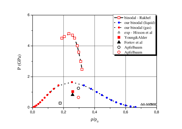
a)

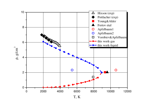
b)

Figure 1: Binodal of iron in coordinates $P$ vs $\rho/\rho_{0}$ (1a) and $\rho$ vs $T$ (1b), respectively. Dashed line with points – this work. Experimental data: open triangles – Hixson [43], dashed line with open squares – Rakhel et al [44], diamonds – Beutl et al [8]. Theoretical estimations of critical point: filled square – Young and Alder [15], filled triangle – Fortov et al [22], open square – Vorob’ev and Apfelbaum [23]; open circles – Apfelbaum [45].

Figure 1 presents binodal of iron in the coordinates $P$ vs $\rho/\rho_{0}$ (1a) and $\rho$ vs $T$ (1b), respectively. Triangles correspond to the experimental data on $0,2$ GPa isobar from Hixson [43], diamonds correspond to the experimental data obtained by the pulse heating of wires from work Beutl et al [8]. Squares correspond to the binodal, obtained experimentally in work of Rakhel with co-authors [44]. Theoretical estimations of critical point parameters obtained by various authors are also shown: the filled square correspond to the calculation using the van der Waals equation of state from Young and Alder [15]; triangle – calculation using the method of corresponding states by Fortov et al [22]; open square – calculation using the similarity law from the work of Vorob’ev and Apfelbaum [23]; open circles – calculation using the Morse potential from the work of Apfelbaum [45]. The dashed curve with dots marks our calculation. As can be seen from figure 1, our calculations for the liquid branch of the binodal are in good agreement with available experimental data [8].

Figure 2 presents binodal of vanadium in the coordinates $\rho$–$T$. Experimental data from fast pulse heating systems are shown: 1 – data at Kiel [5]; 2 – data at $0,3$ GPa at Livermore [5]. Theoretical estimates of the critical point, obtained by various authors: open circle – calculation using the van der Waals equation of state by Young and Alder [15]; filled square – calculation using the method of corresponding states from Fortov et al [22]; filled triangle – calculation using the van der Waals equation of state with soft spheres by Young, 1977 [21]; filled diamond – estimate from experimental data by Martynyuk [11].

Figure 3 presents binodal of gold in the coordinates $\rho$–$T$. The filled triangles correspond to the experimental data on the wire explosion from Kaschnitz et al [46]. Diamond with error bars – experimental estimation of the critical point from Pottlacher et al [10]. Theoretical estimates of the critical point, obtained by various authors: open circle – calculation using the van der Waals equation of state by Young and Alder [15]; filled square – calculation using the method of corresponding states from Fortov et al [22]; open triangle – Morris [42].

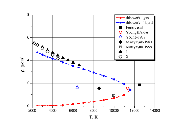
Figure 2: Binodal of vanadium in coordinates $\rho$ vs $T$. Dashed line with points – this work. Experimental data: 1 – data from fast system at Kiel [5]; 2 – data at $0.3$ GPa from fast system at Livermore [5]. Theoretical estimations of critical point: open circle – Young and Alder [15]; filled square – Fortov etal [22]; open triangle – estimate of CP using van der Waals model with soft spheres, Young, 1977 [5]; filled diamond – estimate from experimental data by Martynyuk [11].

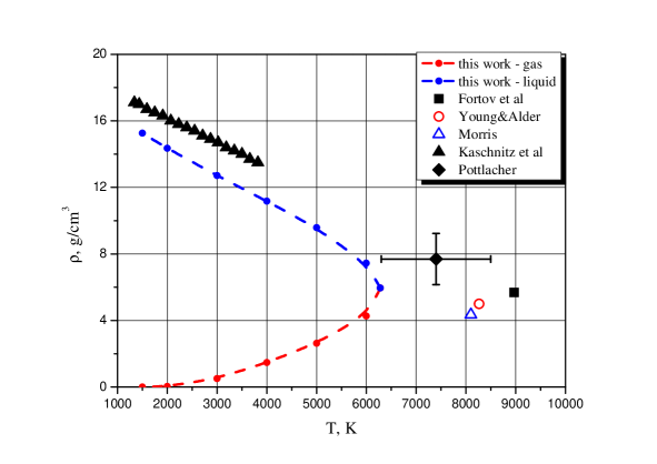
Figure 3: Binodal of gold in coordinates $\rho$ vs $T$. Dashed line with points – this work. Diamond with error bar – experimental estimate of CP by Pottlacher et al [10]. Filled triangles – experimental data of Kaschnitz et al [46]. Open circle – Young and Alder [15]; filled square – Fortov et al [22]; open triangle – Morris [42].

As can be seen from the figures, the results of our calculations in the framework of a rather simple physical model quite well agree with known experimental data for liquid metals in the temperature range from the melting temperature to $T\sim 5000$ K. Various estimations of the critical density for iron give similar values. However, the scatter of estimates for the critical temperature and, especially, for the critical pressure of iron is large. This situation is typical for most transition metals. Our calculations clarify the available data.

As an example, Table 2 presents calculations of the electrical conductivity at the critical point (critical electrical conductivity) for Cu, Ag, Fe, V, and Zn, performed by the Regel-Ioffe formula (12), but with different values of the degree of ”cold ionization” $\alpha$. The index of the symbol of the electrical conductivity $\sigma$ indicates the method of calculation of the $\alpha$ value. Available estimation of the electrical conductivity for iron [44] at the critical point is also presented in Table 2.

Table 2: Electrical conductivity at the critical point for various metals

Metal	$\sigma_{Sc}$, 1/($\Omega$cm)	$\sigma_{HF}$, 1/($\Omega$cm)	$\sigma_{exp}$, 1/($\Omega$cm)
V	2540	2440
Zn	3100	2040
Cu	2520	1660
Ag	2180	1570
Fe	3440	2560	2500 $\pm$ 800

We have performed calculations of the parameters of the critical point for almost all metals of the periodic table. Analysing the obtained results, we noticed some interesting regularities. The unitless parameter $a^{\ast}$ at the critical point is with good precision ($\sim 10\%$) close to $3$ for most metals. From this fact, a simple relation follows for the unitless radius of the Wigner-Seitz cell at the critical point $y_{cr}$, that allows calculating the critical density:

$$y_{cr}=y_{0}+3l_{0}.$$ (13)

From our model, it follows that the ratio of cohesion in the minimum $\Delta E$ (heat of evaporation under normal conditions) to the critical temperature is $\sim 5\div 6$ , thus, follows the Kopp-Lang rule [47]:

$$\Delta E/T_{cr}=const=5\div 6.$$ (14)

Relations (13, 14), obtained ”theoretically”, are peculiar similarity relations binding the critical density and temperature with the evaporation heat, the normal density, and the isothermal bulk modulus.

5 Conclusions

In this paper, we propose a model for calculating the parameters of the critical point and electrical conductivity, as well as binodal of the vapor-liquid phase transition for transition metals (metals with an uncompleted outer electron shell). The model is based on the hypothesis about the decisive role of collective quantum binding energy – cohesion for the description of the interatomic interactions for the metal both in the condensed state, and in the gas state near the critical point. To calculate cohesion of multielectron atoms of the metals, we suggest using the scaling relations known from the literature. The parameters of the critical point are obtained, and the binodals are calculated for transition metals. The critical electrical conductivity for most metals is calculated for the first time.

Final confirmation of the accuracy of calculations within ”thermal” or ”caloric” approaches requires carrying out further experiments. Most likely, it will be experimenting with installations on shock compression and the subsequent adiabatic expansion of porous samples of metals.

6 Acknowledgments

This study was supported by the Russian Science Foundation under the Project No 14-50-00124.

References

- [1] Hirschfelder J.O., Curtiss C.F., Byron Bird R. Molecular Theory of Gases and Liquids. New York: Wiley, 1954.
- [2] Hensel F., Marceca E., Pilgrim W.C. J Phys-Condens Mat 10 (1998) 11395.
- [3] Hensel F. Adv Phys 44 (1995) 3.
- [4] Kikoin I.K., Senchenkov A.P. Fiz Met Metalloved+ 24 (1967) 843.
- [5] Gathers G.R. Rep Prog Phys 49 (1986) 341.
- [6] Pottlacher G. High temperature thermophysical properties of 22 pure metals. Graz: Edition Keiper, 2010.
- [7] Hess H., Kaschnitz E., Pottlacher G. High Pressure Res 12 (1994) 1323.
- [8] Beutl M., Pottlacher G., Jäger H. Int J Thermophys 15 (1994) 1323.
- [9] Seydel U., Fucke W. J Phys F Met Phys 8 (1978).
- [10] Boboridis K., Pottlacher G., Jäger H. Int J Thermophys 20 (1999) 1289.
- [11] Martynyuk M.M. Russ J Phys Chem+ 57 (1983) 810.
- [12] Pottlacher G., Jäger H. J Non-Cryst Solids 205 (1996) 265.
- [13] Nikolaev D.N., Ternovoi V.Y., Pyalling A.A., Filimonov A.S. Int J Thermophys 23 (2002) 1311.
- [14] Emelyanov A.N., Nikolaev D.N., Ternovoi V.Y. High Temp - High Press 37 (2008) 279.
- [15] Young D.A., Alder B.J. Phys Rev A 3 (1971) 364.
- [16] Bushman A.V., Fortov V.E. Phys-Usp+ 140 (1983) 177.
- [17] Likalter A.A. Phys-Usp+ 170 (2000) 831.
- [18] Martynyuk M.M. Russ J Phys Chem+ 72 (1998) 19.
- [19] Martynyuk M.M., Tamanga P.A. High Temp-High Press 31 (1999) 561.
- [20] Blairs S., H. A.M. J Colloid Interf Sci 304 (2006) 549.
- [21] Grosse A.V., Kirschenbaum A.D. J Inorg Nucl Chem 24 (1962) 739.
- [22] Fortov V.E., Dremin A.N., Leont’ev A.A. High Temp+ 13 (1975) 984.
- [23] Apfelbaum E.M., Vorob’ev V.S. J Phys Chem B 119 (2015) 11825.
- [24] Ziman J.M. Principles of the Theory of Solids. London: Cambridge University Press, 1972.
- [25] Apfelbaum E.M. Phys Chem Liq 48 (2010) 534.
- [26] Redmer R., Reinholtz H., Roepke G., Winter R., Noll F., Hensel F. J Phys-Condens Mat 4 (1992) 1659.
- [27] Knyazev D.V., Levashov P.R. Phys Plasmas 21 (2014) 07330.
- [28] Khomkin A.L., Shumikhin A.S. J Exp Theor Phys+ 118 (2014) 72.
- [29] Khomkin A.L., Shumikhin A.S. J Exp Theor Phys+ 121 (2015) 521.
- [30] Khomkin A.L., Shumikhin A.S. Contrib Plasm Phys 56 (2016) 228.
- [31] Banerjia A., Smith J.R. Phys Rev B 37 (1988) 6632.
- [32] Rose J.H., Smith J.R., Guinea F., Ferrante J. Phys Rev B 29 (1984) 2963.
- [33] Clementi E., Roetti C. Atom Data Nucl Data 14 (1974) 177.
- [34] Bardeen J. J Chem Phys 6 (1938) 367.
- [35] Daw M.S., Baskes M.I. Phys Rev B 29 (1983) 6443.
- [36] Rose J.H., Smith J.R., Ferrante J. Phys Rev B 28 (1983) 1835.
- [37] Likalter A.A. Physica A 311 (2002) 137.
- [38] Likalter A.A. Phys Scripta 55 (1997) 114.
- [39] Filippov L.P. Metody rascheta i prognozirovaniya svoistv veshchestv (Methods for Calculating and Predicting the Properties of Substances). Moscow: Moscow State University, 1988.
- [40] Apfelbaum E.M., Vorob’ev V.S. Chem Phys Lett 467 (2009) 318.
- [41] Onufriev S.V. High Temp+ 49 (2011) 205.
- [42] Morris E. AWRE Report. London: UKAEA, 1964.
- [43] Hixson R.S., Winkler M.A., Hodgdon M.L. Phys Rev B 42 (1990) 6485.
- [44] Korobenko V.N., Rakhel A.D. Phys Rev B 85 (2012) 014208.
- [45] Apfelbaum E.M. J Chem Phys 134 (2011) 194506.
- [46] Kaschnitz E., Nussbaumer G., Pottlacher G., Jäger H. Int J Thermophys 14 (1993) 251.
- [47] Lang G. Z Metallkd 68 (1977) 213.