High-Performance Tensor Contraction without Transposition

Abstract

Tensor computations–in particular tensor contraction (TC)–are important kernels in many scientific computing applications. Due to the fundamental similarity of TC to matrix multiplication (MM) and to the availability of optimized implementations such as the BLAS, tensor operations have traditionally been implemented in terms of BLAS operations, incurring both a performance and a storage overhead. Instead, we implement TC using the flexible BLIS framework, which allows for transposition (reshaping) of the tensor to be fused with internal partitioning and packing operations, requiring no explicit transposition operations or additional workspace. This implementation, TBLIS, achieves performance approaching that of MM, and in some cases considerably higher than that of traditional TC. Our implementation supports multithreading using an approach identical to that used for MM in BLIS, with similar performance characteristics. The complexity of managing tensor-to-matrix transformations is also handled automatically in our approach, greatly simplifying its use in scientific applications.

1 Introduction

Tensors are an integral part of many scientific disciplines [38, 28, 3, 19, 18]. At their most basic, tensors are simply a multidimensional collection of data (or a multidimensional array, as expressed in many programming languages). In other cases, tensors represent multidimensional transformations, extending the theory of vectors and matrices. The logic of handling, transforming, and operating on tensors is a common task in many scientific codes, often being reimplemented many times as needed for different projects or even within a single project. Calculations on tensors also often account for a significant fraction of the running time of such tensor-based codes, and so their efficiency has a significant impact on the rate at which the resulting scientific advances can be achieved.

In order to perform a tensor contraction, there are currently two commonly used alternatives: (1) write explicit loops over the various tensor indices (this is the equivalent of the infamous triple loop for matrix multiplication), or (2) “borrow” efficient routines from optimized matrix libraries such as those implementing the BLAS interface [20, 9, 8]. Choice (1) results in a poorly-performing implementation if done naively due to the lack of optimizations for cache reuse, vectorization, etc. as are well-known in matrix multiplication (although for a high-performance take on this approach see GETT [32] as discussed in 8), and also generally requires hardcoding the specific contraction operation, including the number of indices on each tensor, which indices are contracted, in which order indices are looped over, etc. This means that code cannot be efficiently reused as there are many possible combinations of number and configuration of tensor indices. Choice (2) may provide for higher efficiency, but requires mapping of the tensor operands to matrices which involves both movement of the tensor data in memory and often this burden falls on the user application. Alternatively, the tensors may be sliced (i.e. low-dimensional sub-tensors are extracted) and used in matrix multiplication, but this again has drawbacks as discussed below.

Several libraries exist that take care of part of this issue, namely the tedium of encoding the logic for treating tensors as matrices during contractions. For example, the MATLAB Tensor Toolbox [2] provides a fairly simple means for performing tensor contractions without exposing the internal conversion to matrices. The NumPy library [35] provides a similar mechanism in the Python language. Both libraries still rely on the mapping of tensors to matrices and the unavoidable overhead in time and space thus incurred. In many cases, especially in languages common in high-performance computing such as FORTRAN and C, a pre-packaged solution is not available and the burden of implementing tensor contraction is left to the author of the scientific computing application, although several libraries for tensor contraction in C++ have recently been developed [10, 30, 5, 6].

A natural solution to this problem is to create a dedicated tensor library implementing a high-performance, “native” tensor contraction implementation (without the use of the BLAS), but with similar optimizations for cache reuse, vectorization, etc. as those used for matrix multiplication. For a particular instance of a tensor contraction this is a feasible if not tedious task, using existing techniques from dense linear algebra. However, making a general run-time tensor library is another proposition altogether, as it is highly desirable for such a library to handle any number of tensor indices, as well as number, order, and position of contracted indices. Static code transformation/generation techniques such as in Built-to-Order BLAS [4], DxTer [24], and GETT [32] can produce highly efficient code but are much less flexible since they require tensor dimensionality and ordering (and in many cases, sizes) to be fixed at compile time. Since the number of possible contraction types grows exponentially with the number of indices, explicitly treating each instance of tensor contraction is an uphill endeavor in large applications with many tensor contraction instances. Not requiring a code-generation stage is also highly beneficial to rapid prototyping of new algorithms that use tensor contraction, while having a high-performance general tensor contraction library can often turn prototypes into useful production code.

The newly-developed BLIS framework [37, 29, 36] implements matrix operations with a very high degree of efficiency, including a legacy BLAS interface. However, unlike common BLAS libraries, especially commercial libraries such as Intel’s Math Kernel Library, BLIS exposes the entire internal structure of algorithms such as matrix multiplication, down to the level of the micro-kernel, which is the only part that must be implemented in highly-optimized assembly language. In addition to greatly reducing the effort required to build a BLAS-like library, the structure of BLIS allows one to view a matrix operation as a collection of independent pieces. Matrix multiplication (and other level 3 BLAS operations) are the default algorithms provided by BLIS, but one may also use the available pieces to build a custom framework for purposes beyond traditional dense linear algebra, examples of which are given in [41] and [17]. We will illustrate exactly how the flexibility of this approach may be used to implement high-performance tensor contraction by breaking through the traditionally opaque matrix multiplication interface. The benefits of this approach are detailed in 9, where our new algorithm, Block-Scatter-Matrix Tensor Contraction (BSMTC), is compared to a traditional tensor contraction approach, Transpose-Transpose-GEMM-Transpose (TTGT) as implemented by the Tensor Toolbox.

The specific contributions of this paper are:

• A novel logical mapping from general tensor layouts to a non-standard (neither row-major nor column-major) matrix layout.

• Implementations of key BLIS kernels using this novel matrix layout, eliminating the need for explicit transposition of tensors while retaining a matrix-oriented algorithm.

• A new BLIS-like framework incorporating these kernels that achieves high performance for tensor contraction and does not require external workspace.

• Efficient multithreading of tensor contraction within the aforementioned framework.

2 The Big Idea: Tensors As Matrices

Before developing the theory of matrix multiplication and tensor contraction in detail, let us first examine the high-level concepts which guide our implementation of tensor contraction. First, we may introduce tensors quite simply as the multi-dimensional extension of scalars (0-dimensional tensors), vectors (1-dimensional tensors), and matrices (2-dimensional tensors), or similarly as multi-dimensional arrays. Tensor contraction is the also natural extension of matrix multiplication to tensors, where for each index (dimension) in the two input and the single output matrix we substitute one or more tensor dimensions. Thus, a contraction of a 7-dimensional tensor $\mathscr{A}$ by a 5-dimensional tensor $\mathscr{B}$ into a 6-dimensional tensor $\mathscr{C}$ is in fact mathematically a matrix multiplication in disguise if we say that for example, $\mathscr{A}$ is in fact 4-dimensional by 3-dimensional (for some partition of the 7 dimensions into groups of 4 and 3), $\mathscr{B}$ is 3-dimensional by 2-dimensional, and $\mathscr{C}$ is merely 4-dimensional by 2-dimensional. The problem with mapping tensor contraction to matrix multiplication in practice is that the data layout of tensors in memory is much more flexible and varied than for matrices, and a direct mapping is generally not possible.

Since matrix multiplication and tensor contraction are really the same thing, then, the obvious question is, “how can existing high-performance matrix multiplication algorithms be used for tensor contraction?” The trick is to relate the single matrix dimensions, which are usually described by a length (number of elements), and a stride (distance between elements), to a whole group of tensor dimensions (especially when the number of tensor dimensions is not known beforehand). As we will show in the following sections, this relationship between matrices and tensors is cleanly and efficiently accomplished by creating a specialized matrix layout instead of simple scalar strides, which by design describes the physical data layout of a specified tensor. An existing matrix multiplication algorithm can then use this layout to access matrix elements without knowing anything about tensors or tensor contraction. We will demonstrate that this approach yields a relatively simple and highly efficient tensor contraction algorithm.

3 Matrix Multiplication

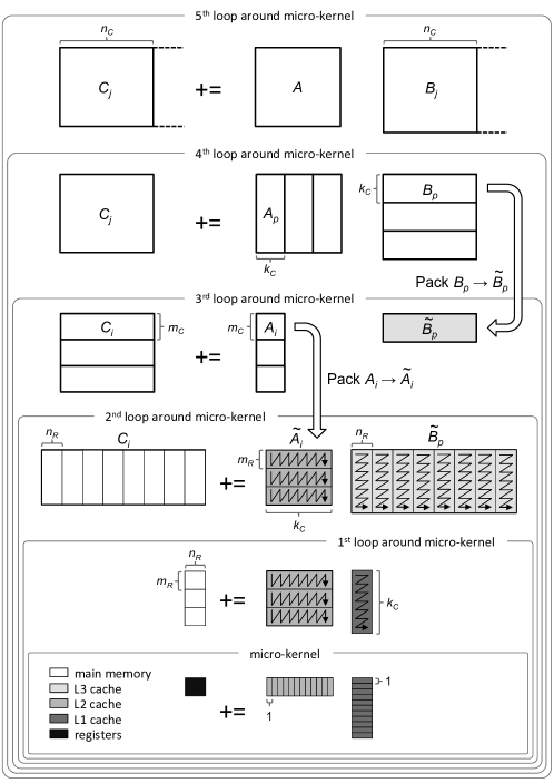
Figure 1: The structure of a matrix multiplication operation using the BLIS approach. Figure from https://github.com/flame/blis/wiki/Multithreading, used with permission.

Let us first review the basic techniques used in high-performance matrix multiplication, expressed generally as $C\coloneqq\alpha AB+\beta C$. The matrices $A$, $B$, and $C$ are $m\times k$, $k\times n$, and $m\times n$ respectively. We refer to the length and width of each matrix as its shape, and refer to individual elements of each matrix as $A_{ip}$, $C_{ij}$, etc. where $0\leq i<m$, $0\leq j<n$, and $0\leq p<k$. Written element-wise, the basic matrix multiplication operation is then $C_{ij}\coloneqq\alpha\sum_{p=0}^{k-1}A_{ip}\cdot B_{pj}+\beta C_{ij}\,\forall\,(i,j)\in m\times n$. In this context, $m\times n$ is a shorthand for the Cartesian product of the ranges $[0,m)$ and $[0,n)$, i.e. $m\times n=\{(i,j)\,|\,0\leq i<m\,\vee\,0\leq j<n\}$. The use of Cartesian products over integers to denote such sets will be used extensively. This element-wise definition of matrix multiplication is critical to relating it to tensor contraction, although for brevity we will assume $\alpha=1$ and $\beta=0$ henceforth.

Most current high-performance implementations follow the approach pioneered by Goto [11, 12], in which the matrices are successively partitioned (sub-divided) into panels (sub-matrices), labeled for example $A_{i}$, $B_{p}$, and $C_{j}$ in blis, which are designed to fit into the various levels of the cache hierarchy. The panels of $A$ and $B$ are packed (copied) into temporary buffers $\tilde{A}_{i}$ and $\tilde{B}_{p}$ in a special storage format to facilitate vectorization and memory locality. The size of these panels are determined by cache blocking parameters $m_{C}$, $n_{C}$, and $k_{C}$, such that $\tilde{A}_{i}$ (which stores an $m_{C}\times k_{C}$ panel of $A$) is retained in the L2 cache while $\tilde{B}_{p}$ (which stores a $k_{C}\times n_{C}$ panel of $B$) is retained in the L3 cache (if present). In the original Goto approach, these “pack buffers” are then fed into an inner kernel which performs the actual matrix multiplication sub-problem, and which is typically written in hand-optimized assembly code.

The BLIS approach [37] implements the inner kernel instead in terms of a much smaller and easier to write micro-kernel. In this approach, the panels of $A$ and $B$ as stored in $\tilde{A}_{i}$ and $\tilde{B}_{p}$ are further partitioned according to register block sizes $m_{R}$ and $n_{R}$ such that a pair of $m_{R}\times k_{C}$ and $k_{C}\times n_{R}$ slivers of $\tilde{A_{i}}$ and $\tilde{B}_{p}$, respectively, fit into the L1 cache. The micro-kernel then uses these slivers to update a small $m_{R}\times n_{R}$ micro-tile of $C$, which is maintained in machine registers. These five cache and register block sizes give rise to five loops (written in C or another relatively high-level language) around the micro-kernel, as illustrated in blis.

The major logical and computational operations involved in the BLIS approach are then: (1) partitioning of matrix operands, (2) packing of matrix panels (as a set much smaller matrix slivers) into specially-formatted buffers, and (3) invocation of the micro-kernel. We will see these operations can be implemented in the context of general tensors instead of matrices in later sections, in order to make use of the highly-tuned BLIS framework for tensor contraction.

4 Tensor Contraction

A general $d$-dimensional tensor $\mathscr{A}\in\mathbb{R}^{n_{u_{0}}\times\ldots\times n_{u_{d-1}}}$ is defined as the set of scalar elements indexed by the set of indices $u_{0}\ldots u_{d-1}$,

(1) $$\mathscr{A}\equiv\{\mathscr{A}_{u_{0}\ldots u_{d-1}}\in\mathbb{R}\,|\,(u_{0},\ldots,u_{d-1})\in n_{u_{0}}\times\ldots\times n_{u_{d-1}}\}$$

Often, the indices of a tensor ($u_{0},\ldots,u_{d-1}$) will be given more convenient labels, such as in $\mathscr{A}_{abc\ldots}$, while the length of the corresponding tensor dimensions will be denoted $n_{a}$, $n_{b}$, etc. Indices which have the same label in more than one tensor in any tensor expression must share the same value, and the lengths of the corresponding dimensions in each tensor must be identical. For example, in an expression such as $\mathscr{A}_{cfbd}\cdot\mathscr{B}_{fea}$, the length of the index $f$, $n_{f}$, must be the same in $\mathscr{A}$ and $\mathscr{B}$, and only pairs of elements with the same value of $f$ in $\mathscr{A}$ and $\mathscr{B}$ enter the expression.

Tensor contraction generalizes the concept of matrix multiplication to higher dimensions (numbers of indices), just as tensors generalize the notion of matrices. Given two input tensors $\mathscr{A}$ and $\mathscr{B}$ of dimension $d(\mathscr{A})$ and $d(\mathscr{B})$, respectively, and an output tensor $\mathscr{C}$ of dimension $d(\mathscr{C}$), a tensor contraction is specified by first selecting ordered sets of $d_{P}=(d(\mathscr{A})+d(\mathscr{B})-d(\mathscr{C}))/2$ dimensions each from $\mathscr{A}$ and from $\mathscr{B}$ and labeling the indices of the dimensions in both sets as $p_{0}\ldots p_{d_{P}-1}$. Since the indices are labeled the same in both tensors, their values must be the same (i.e. the indices are bound). Similarly, the remaining dimensions of $\mathscr{A}$ and an ordered set of $d_{I}=(d(\mathscr{A})+d(\mathscr{C})-d(\mathscr{B}))/2$ dimensions in $\mathscr{C}$ have their indices labeled $i_{0}\ldots i_{d_{I}-1}$. Finally, the remaining $d_{J}=(d(\mathscr{B})+d(\mathscr{C})-d(\mathscr{A}))/2$ dimensions in $\mathscr{B}$ and $\mathscr{C}$ are arranged in a selected relative order and their indices labeled $j_{0}\ldots j_{d_{J}-1}$. The tensor contraction operation is then given element-wise by,

$$\mathscr{C}_{\pi_{C}(i_{0}\ldots i_{d_{I}-1}j_{0}\ldots j_{d_{J}-1})}\coloneqq\underset{p_{0},\ldots,p_{d_{P}-1}=0}{\sum^{n_{p_{0}}-1,\ldots,n_{pd_{P}-1}-1}}\mathscr{A}_{\pi_{A}(i_{0}\ldots i_{d_{I}-1}p_{0}\ldots p_{d_{P}-1})}\cdot\mathscr{B}_{\pi_{B}(p_{0}\ldots p_{d_{P}-1}j_{0}\ldots j_{d_{J}-1})}$$

(2) $$\forall(i_{0},\ldots,i_{d_{I}-1},j_{0},\ldots,j_{d_{J}-1})\in n_{i_{0}}\times\ldots\times n_{i_{d_{I}-1}}\times n_{j_{0}}\times\ldots\times n_{j_{d_{J}-1}}$$

where $\cdot$ is scalar multiplication and $\pi_{A}$, $\pi_{B}$, and $\pi_{C}$ are permutations (reorderings) of their respective indices. These permutations are necessary to write the general definition because dimensions may have been chosen in any position and in any relative order when determining the labeling of indices. To simplify the notation, the sets of index labels $i_{0}\ldots i_{d_{I}-1}$, $j_{0}\ldots j_{d_{J}-1}$, and $p_{0}\ldots p_{d_{P}-1}$ are denoted as index bundles $I$, $J$, and $P$, respectively. The $I$ and $J$ bundles contain the uncontracted (free) indices, while the $P$ bundle contains the contracted (bound) indices. Additionally, we will make use of Einstein notation, such that the indices in the $P$ bundle, since they appear twice on the right-hand side, are implicitly summed over, and the remaining indices are implicitly iterated over. Using these simplifications, the general tensor contraction becomes,

(3) $$\mathscr{C}_{\pi_{C}(IJ)}\coloneqq\mathscr{A}_{\pi_{A}(IP)}\cdot\mathscr{B}_{\pi_{B}(PJ)}$$

Now the connection to matrix multiplication is readily apparent. Simplifying the element-wise definition of matrix multiplication in the same way gives,

(4) $$C_{ij}=A_{ip}\cdot B_{pj}$$

This is identical to tensor contraction except that, (1) the index bundles $I$, $J$, and $P$ may contain more than one index, while $i$, $j$, and $p$ are single indices, and (2), the indices in the tensor contraction case may be arbitrarily ordered by the permutation operators. In the matrix case, permutation of the indices in $A$, $B$, or $C$ amounts to simple matrix transposition, but in the tensor case indices from different bundles may be interspersed as well as transposed overall. If each of the tensor dimensions is $\mathscr{O}(N)$, then the tensor contraction operation requires $\mathscr{O}(N^{d_{I}+d_{J}+d_{P}})$ FLOPs (floating point operations), which is the same number of operations as a matrix multiplication with $m=N^{d_{I}}$, $n=N^{d_{J}}$, and $k=N^{d_{P}}$.

5 The Traditional Approach

In order to introduce both existing and our novel approaches to tensor contraction, let us consider a concrete, if simple, example. Say that we have tensors $\mathscr{A}\in\mathbb{R}^{2\times 4\times 3\times 3}$, $\mathscr{B}\in\mathbb{R}^{4\times 4\times 6}$, and $\mathscr{C}\in\mathbb{R}^{6\times 3\times 2\times 3\times 4}$, and we wish to compute the tensor contraction,

(5) $$\mathscr{C}_{abcde}\coloneqq\mathscr{A}_{cfbd}\cdot\mathscr{B}_{fea}$$

The tensor contraction may also be written in the form of (3) as,

(6) $$\mathscr{C}_{\pi_{C}(cdbae)}\coloneqq\mathscr{A}_{\pi_{A}(cdbf)}\cdot\mathscr{B}_{\pi_{B}(fae)}$$

where it is clear that in this case the index bundles as defined in the previous section are $I=cdb$, $J=ae$, and $P=f$, and the action of the permutation operators is to reorder the indices to the order of (5).

The most common traditional approach to tensor contraction is to use the similarities noted above between tensor contraction and matrix multiplication to implement the former in terms of the latter, making use of highly-tuned matrix multiplication routines such as through the BLAS interface. To see how this is possible, assume for a moment that we had picked a slightly different tensor contraction such that $\pi_{A}$, $\pi_{B}$, and $\pi_{C}$ were the identity permutations,

(7) $$\mathscr{\tilde{C}}_{cdbae}\coloneqq\mathscr{\tilde{A}}_{cdbf}\cdot\mathscr{\tilde{B}}_{fae}$$

with the same dimension length for each index such that $\tilde{\mathscr{C}}\in\mathbb{R}^{2\times 3\times 3\times 6\times 4}$ etc.

Let us assume also that the tensors are laid out in general column-major order, which is similar to the well-known column-major order for matrices. In this format, the entries of each tensor are arranged in memory contiguously and with increasing colexicographic order of the indices. For example, the locations of elements of $\tilde{\mathscr{C}}$ relative to the base address are given by,

(8) $$loc(\tilde{\mathscr{C}}_{cdbae}) = c+d\cdot n_{c}+b\cdot n_{c}n_{d}+a\cdot n_{c}n_{d}n_{b}+e\cdot n_{c}n_{d}n_{b}n_{a}$$

$$= c+d\cdot n_{c}+b\cdot n_{c}n_{d}+(a+e\cdot n_{a})\cdot n_{c}n_{d}n_{b}$$

where scalar multiplication of lengths is assumed. It is assumed that the values of the indices run over their entire range in this and similar expressions (i.e. $(a,b,c,d,e)\in n_{a}\times n_{b}\times n_{c}\times n_{d}\times n_{e}$ for (8)). Similarly, the locations of the indices in $\tilde{\mathscr{A}}$ and $\tilde{\mathscr{B}}$ are given by,

(9) $$loc(\mathscr{\tilde{A}}_{cdbf}) = c+d\cdot n_{c}+b\cdot n_{c}n_{d}+f\cdot n_{c}n_{d}n_{b}$$

(10) $$loc(\mathscr{\tilde{B}}_{fae}) = f+a\cdot n_{f}+e\cdot n_{f}n_{a}$$

$$= f+(a+e\cdot n_{a})\cdot n_{f}$$

The range of values $c+d\cdot n_{c}+b\cdot n_{c}n_{d}$ for $(c,d,b)\in n_{c}\times n_{d}\times n_{b}=2\times 3\times 3$ is simply the ordered range of values $0\leq\bar{I}<n_{\bar{I}}$ for $n_{\bar{I}}=n_{c}n_{d}n_{b}=18$, thanks to column-major ordering. When multiple indices may be collapsed into the range of a single contiguous index, they are said to be sequentially contiguous. Similarly the range $a+e\cdot n_{a}$ for $(a,e)\in n_{a}\times n_{e}=6\times 4$ is identical to $0\leq\bar{J}<n_{\bar{J}}=n_{a}n_{e}=24$, and the possible values of $f$ are trivially the range $0\leq\bar{P}<n_{\bar{P}}=n_{f}=4$. Furthermore, since the value of the combined index $\bar{I}$ is the same for identical values of $c$, $d$, and $b$ in both the $\mathscr{A}$ and $\mathscr{B}$ tensors, they may both be addressed by the same linearized index $\bar{I}$, and the same is true of $\bar{J}$ and (trivially) $\bar{P}$ as well. Thus, the tensors $\mathscr{\tilde{A}}$, $\tilde{\mathscr{B}}$, and $\mathscr{\tilde{C}}$ are structurally equivalent to matrices $\tilde{A}$, $\tilde{B}$, and $\tilde{C}$ that are $n_{\bar{I}}\times n_{\bar{P}}$, $n_{\bar{P}}\times n_{\bar{J}}$, and $n_{\bar{I}}\times n_{\bar{J}}$, respectively. The tilde denotes that the tensor is compatible with a matrix layout and vice versa. The tensor contraction is also functionally equivalent (i.e. it results in the same values in the same locations in memory) to the matrix multiplication,

(11) $$\tilde{C}_{\bar{I}\bar{J}}\coloneqq\tilde{A}_{\bar{I}\bar{P}}\cdot\tilde{B}_{\bar{P}\bar{J}}$$

Thus, the tensor contraction may be accomplished by simply performing a matrix multiplication with the proper parameters. This is possible whenever the indices in each of the bundles $I$, $J$, and $P$ in the general tensor contraction definition are sequentially contiguous and identically ordered in each tensor (assuming general column-major storage; the value of the linearized index must simply be the same for identical values of the tensor indices in both tensors in the general case)–both conditions together forming the condition of linearizability–so that they may be replaced by linearized indices $\bar{I}$, $\bar{J}$, and $\bar{P}$ in a matrix multiplication, where the over-bar denotes linearization.

But what about our original tensor contraction? In that case, it is easy to see that the indices are not sequentially contiguous (for example $b$ does not follow $d$ in $\mathscr{C}$), nor are they identically ordered in all cases (for example, $b$ is ordered before $c$ in $\mathscr{C}$, but $c$ is before $b$ in $\mathscr{A}$). In this case, the tensors may be transposed (reordered) in memory such that the indices become sequentially contiguous and may be linearized. Using our example, we may copy the elements in $\mathscr{A}$ to their corresponding locations in $\tilde{\mathscr{A}}$, and the elements in $\mathscr{B}$ to $\tilde{\mathscr{B}}$, perform the matrix multiplication, then copy the resulting elements of $\tilde{\mathscr{C}}$ to their final locations in $\mathscr{C}$. This approach is commonly termed the TTGT (transpose-transpose-GEMM-transpose) approach, after the GEMM matrix multiplication function in BLAS. In general, if we define the tensor contraction operation as in (3) then we may implement TTGT using the algorithm in TTDT, assuming that the temporary tensors $\mathscr{\tilde{A}}$, $\tilde{\mathscr{B}}$, and $\mathscr{\tilde{C}}$ are stored in general column-major order.

1:procedure TTGT($\alpha,\mathscr{A}_{\pi_{A}(IP)},\mathscr{B}_{\pi_{B}(PJ)},\beta,\mathscr{C}_{\pi_{C}(IJ)}$)

2:     Transpose $\tilde{\mathscr{A}}_{IP}\coloneqq\mathscr{A}_{\pi_{A}(IP)}$

3:     Transpose $\tilde{\mathscr{B}}_{PJ}\coloneqq\mathscr{B}_{\pi_{B}(PJ)}$

4:     $\tilde{C}_{\bar{I}\bar{J}}\coloneqq\alpha\sum_{\bar{P}=0}^{n_{\bar{P}}}\tilde{A}_{\bar{I}\bar{P}}\cdot\tilde{B}_{\bar{P}\bar{J}}$

5:     Transpose and sum $\mathscr{C}_{\pi_{C}(IJ)}\coloneqq\tilde{\mathscr{C}}_{IJ}+\beta\mathscr{C}_{\pi_{C}(IJ)}$

6:end procedure

Figure 2: Schematic implementation of the TTGT approach for tensor contraction. Notational details explained in text.

This method has been used to implement tensor contraction in a vast number of scientific applications over the past few decades, and is the implementation used by popular tensor packages such as NumPy [35] and the MATLAB Tensor Toolbox [2]. However, there are some drawbacks to this approach:

• The storage space required is increased by a factor of two, since full copies of $\mathscr{A}$, $\mathscr{B}$, and $\mathscr{C}$ are required. This storage space may either be allocated inside the tensor contraction routine or supplied as workspace by the user, complicating user interfaces. This deficiency is similar to that encountered in traditional implementations of Strassen’s algorithm for matrix multiplication [17].

• The tensor transpositions require a (sometimes quite significant) amount of time relative to the matrix multiplication step even after optimization of the transposition step, as evidenced by the results of the present work and elsewhere in the literature [15, 14, 32]. As an applied example, after aggressively reordering operations to reduce the number of transpositions needed in the NCC quantum chemistry program [25] (transpositions can be elided if the ordering required for one operation matches that required for the next), we still measure 15-50% of the total program time spent in tensor transposition. This overhead is especially onerous in methods such as CCSD(T) [27, 1], where storage size (and hence transposition cost) scales as $\mathscr{O}(N^{6})$ but computation scales only as $\mathscr{O}(N^{7})$.

• If a comprehensive tensor contraction interface is not available (e.g. in FORTRAN or C), or if tensor transposition must be otherwise handled by the calling application to ensure efficiency, significant algorithmic and code complexity is required which increases programmer burden and the incidence of errors, while obscuring the scientific algorithms in the application. Although it is hard to measure this deficiency of the TTGT approach quantitatively, the long history in the literature dealing with optimization and implementation of TTGT indicates the level of effort implied by this approach.

These deficiencies motivate our implementation of a “native” (i.e. acting directly on general tensors) high-performance tensor contraction algorithm.

6 New Matrix Representations of Tensors

6.1 The Scatter-Matrix Layout

In order to eliminate the need for costly tensor transpositions, it is necessary to eschew the standard BLAS interface for matrix multiplication. However, we also wish to make use of highly-tuned algorithms for matrix multiplication that, by the mathematical equivalence between matrix multiplication and tensor contraction, should be applicable. The BLIS framework gives us an opportunity to do just this. In 3, we noted that the only operations required in the BLIS framework are (1) matrix partitioning, (2) packing of matrix panels as slivers, and (3) invoking the micro-kernel. The fundamental question is then, “how can we perform these operations without changing the data layout (transposing) the tensors?”

Going back to our example contraction, let us look at how the tensors are laid out in the non-sequentially contiguous case and relate that to a matrix representation. Focusing on the $\mathscr{C}$ tensor, the indices are grouped into bundles as $I=cdb$ and $J=ae$, while the tensor elements are laid out in general column-major order according to the ordering $\mathscr{C}_{abcde}$. As for $\mathscr{\tilde{C}}$, we can easily compute the locations of tensor elements in $\mathscr{C}$,

(12) $$loc(\mathscr{C}_{abcde}) = a+b\cdot n_{a}+c\cdot n_{a}n_{b}+d\cdot n_{a}n_{b}n_{c}+e\cdot n_{a}n_{b}n_{c}n_{d}$$

$$= (c\cdot n_{a}n_{b}+d\cdot n_{a}n_{b}n_{c}+b\cdot n_{a})+(a+e\cdot n_{a}n_{b}n_{c}n_{d})$$

where in the second equality the terms have been grouped by index bundle. The values for either subexpression do not form a simple, contiguous range that can be represented by a single linearized index. However, we can compare this expression to the locations for the transposed tensor $\tilde{\mathscr{C}}$,

(13) $$loc(\tilde{\mathscr{C}}_{cdbae}) = (c+d\cdot n_{c}+b\cdot n_{c}n_{d})+(a+e\cdot n_{a})\cdot n_{c}n_{d}n_{b}$$

and also to the locations of the matricized form $\tilde{C}$, which we know has the same element locations as $\tilde{\mathscr{C}}$,

(14) $$loc(\tilde{C}_{\bar{I}\bar{J}}) = \bar{I}+\bar{J}\cdot n_{\bar{I}}$$

Since $n_{\bar{I}}=n_{c}n_{d}n_{b}$, we have $\bar{I}=c+d\cdot n_{c}+b\cdot n_{c}n_{d}$ and $\bar{J}=a+e\cdot n_{a}$. Thus, given some values of $\bar{I}$ and $\bar{J}$, we can compute the values of $c$, $d$, $b$, $a$, and $e$, and from those we can finally compute the element location in the unmodified $\mathscr{C}$ tensor. Performing this computation for each individual element is likely not efficient, so the relationship between the tensor and matrix layout may be saved in a row scatter vector $rscat(\mathscr{C})$, which gives the sum $c\cdot n_{a}n_{b}+d\cdot n_{a}n_{b}n_{c}+b\cdot n_{a}$ for each value of $\bar{I}$, and a column scatter vector $cscat(\mathscr{C})$, which gives the sum $a+e\cdot n_{a}n_{b}n_{c}n_{d}$ for each value of $\bar{J}$. For our example, we can compute these scatter vectors as,

(15) $$rscat_{\bar{I}}(\mathscr{C}) = c\cdot n_{a}n_{b}+d\cdot n_{a}n_{b}n_{c}+b\cdot n_{a}$$

$$= \left(\bar{I}\mod n_{c}\right)\cdot n_{a}n_{b}+\left(\frac{\bar{I}}{n_{c}}\mod n_{d}\right)\cdot n_{a}n_{b}n_{c}$$

$$+\left(\frac{\bar{I}}{n_{c}n_{d}}\mod n_{b}\right)\cdot n_{a}$$

(16) $$cscat_{\bar{J}}(\mathscr{C}) = a+e\cdot n_{a}n_{b}n_{c}n_{d}$$

$$= \left(\bar{J}\mod n_{a}\right)+\left(\frac{\bar{J}}{n_{a}}\mod n_{e}\right)\cdot n_{a}n_{b}n_{c}n_{d}$$

The general location of elements in an $n_{\bar{I}}\times n_{\bar{J}}$ matrix $C$ may then be given in the tensor layout of $\mathscr{C}$ as,

(17) $$loc(C_{\bar{I}\bar{J}})=rscat_{\bar{I}}(\mathscr{C})+cscat_{\bar{J}}(\mathscr{C})$$

We call this additive formula for the locations of tensor elements mapped to matrix elements and the associated scatter vectors the scatter-matrix layout, in which the elements of a tensor stored in its natural physical layout may be addressed as if they were a matrix. For our example $\mathscr{C}$, the values of the scatter vectors are illustrated in bsm. For tensor contraction, the scatter vectors $rscat(\mathscr{A})$ and $rscat(\mathscr{C})$ are defined for each value of $\bar{I}$, while the scatter vectors $cscat(\mathscr{B})$ and $cscat(\mathscr{C})$ are defined for each value of $\bar{J}$, and $cscat(\mathscr{A})$ and $rscat(\mathscr{B})$ for each value of $\bar{P}$.

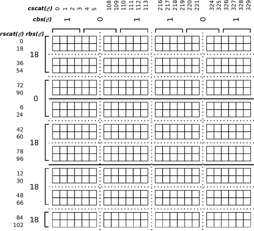
Figure 3: Example of a block-scatter-matrix layout (see 6.2) for the tensor $\mathscr{C}_{abcde}\in\mathbb{R}^{6\times 3\times 2\times 3\times 4}$ with a general column-major data layout (giving strides of 1, 6, 18, 36, and 108). The matrix representation is $C_{\bar{I}\bar{J}}$ for the bundles $I=cdb$ and $J=ae$. The blocking parameters are $m_{R}=n_{R}=4.$ Note that in this case the dimensions $c$ and $d$ are sequentially contiguous and so a regular stride can be maintained for larger blocks.

In general, a tensor may be stored in general column-major order, but also in the similar general row-major order or in any other layout that preserves the uniqueness of elements. The location of elements in a generic layout for $\mathscr{C}$ may be described by a set of index strides, $s(\mathscr{C})$. The location of elements in $\mathscr{C}$ is then,

(18) $$loc(\mathscr{C}_{IJ})=i_{0}\cdot s_{i_{0}}(\mathscr{C})+\ldots+i_{d_{I}-1}\cdot s_{i_{d_{I}-1}}(\mathscr{C})+j_{0}\cdot s_{j_{0}}(\mathscr{C})+\ldots+j_{d_{J}-1}\cdot s_{j_{d_{J}-1}}(\mathscr{C})$$

Unlike the dimension lengths, the strides must always be denoted in reference to a particular tensor because their value for indices which are labeled the same in multiple tensors does not need to agree for each tensor. For our example $\mathscr{C}$ we have $(s_{a}(\mathscr{C}),s_{b}(\mathscr{C}),s_{c}(\mathscr{C}),s_{d}(\mathscr{C}),s_{e}(\mathscr{C}))=(1,6,18,36,108)$. The scatter vectors for a generic layout may also be simply computed,

(19) $$rscat_{\bar{I}}(\mathscr{A})=i_{0}\cdot s_{i_{0}}(\mathscr{C})+\ldots+i_{d_{I}-1}\cdot s_{i_{d_{I}-1}}(C)$$

and similarly for the other scatter vectors.

Turning to the operations necessary to implement the BLIS framework, we can see that the first, matrix partitioning, is trivially implemented by partitioning of the row and/or scatter vectors. For example, the top-right quadrant of a matrix in the scatter-matrix layout may be represented by a sub-matrix with the first half of the full row scatter vector and the second half of the full column scatter vector. The $A$, $B$, and $C$ matrices (matrix representations of $\mathscr{A}$, $\mathscr{B}$, and $\mathscr{C}$ in the scatter-matrix layout) may then be partitioned as much as is necessary while maintaining their scatter-matrix layouts, with essentially no overhead.

For the packing operations, the usual kernels as implemented in BLIS cannot be used, because they assume a general matrix layout, with a constant row and column stride (as in the general tensor layout described above). The scatter-matrix layout, though, does not have a constant stride as can be seen in bsm. A new packing kernel is required that takes row and column scatter vectors and loads elements accordingly. We have implemented such a packing kernel for general scatter-matrix layouts. This packing kernel is not as efficient as the “normal” matrix packing kernel because the scatter-matrix layout inhibits vectorized loads of elements and requires a higher memory bandwidth due to the need to read the scatter vector entries.

Finally, when invoking the micro-kernel, the scatter-matrix layout cannot be used directly. Because the micro-kernel is hand-written in assembly code, and assumes constant row and column strides for $C$, the micro-kernel must be invoked to write to a small temporary buffer (of size $m_{R}\times n_{R}$), and then the values from this buffer written out to memory according the the scatter-matrix layout of $C$. This is again a source of inefficiency as the micro-kernel is normally tuned to write out the elements of $C$ using vector writes. The micro-kernel does not need to be modified for scatter-matrix layouts of $A$ and $B$ because the packing operations write the values in the buffers $\tilde{A}_{i}$ and $\tilde{B}_{p}$ in a fixed layout independent of the input layout.

The implementation of tensor contraction using the BLIS framework augmented by scatter-matrix layouts for $A$, $B$, and $C$ with concordant packing kernels and micro-kernel adjustments is termed the Scatter-Matrix Tensor Contraction (SMTC) algorithm. The next section extends the scatter-matrix layout and SMTC to avoid most of the inefficiency incurred by the use of scatter vectors in the packing and micro-kernel operations.

6.2 The Block-Scatter-Matrix Layout

Since the micro-kernel is the basic unit of work in BLIS, the size of a micro-kernel update defines a natural blocking of the matrix dimensions $m$ and $n$. These block sizes are denoted $m_{R}$ and $n_{R}$ and are usually 4, 6, or 8 for double-precision real numbers. So, while the values of the scatter vectors $rscat(\mathscr{C})$ and $cscat(\mathscr{C})$, are in general not “well-behaved” (monotonically increasing, regularly spaced, etc.) over their entire range which would allow a regular scalar stride to be used instead, they may often be well-behaved for short stretches.

For example, $cscat(\mathscr{C})$ for our sample tensor contraction as calculated from (16) begins with the sequence $0,1,\ldots,n_{a}-1=5$, then jumps up to $n_{a}n_{b}n_{c}n_{d}=108$, continues $108,109,\ldots 108+n_{a}-1$=113, jumps again and so on. So, for small stretches that don’t cross one of the large jumps, $C_{\bar{I}\bar{J}}$ behaves very much like a row-major matrix with a unit “stride” for $\bar{J}$. Similarly, for small stretches of $\bar{I}$, $rscat(\mathscr{C})$ also behaves as if it were a constant stride of $n_{a}n_{b}=18$.

Thus, when $C_{\bar{I}\bar{J}}$ is partitioned into $m_{R}\times n_{R}$ micro-tiles, it is quite possible that the ranges of $\bar{I}$ and $\bar{J}$ for many of these micro-tiles may fall entirely into one of these constant stride regions. In fact, the fraction of micro-tiles that do so is 53% for our example, and generally a much higher fraction for real problems with larger tensor dimensions. When a micro-tile of $C_{\bar{I}\bar{J}}$ has constant strides then it may be fed directly into the micro-kernel without writing to a temporary buffer first. To make use of this optimization, a value is stored for each $m_{R}$-length block of $rscat(\mathscr{C})$ and each $n_{R}$-length block of $cscat(\mathscr{C})$ which is either the stride for this block, when it falls in a region of constant stride, or the value 0 to denote that no such stride exists. These values are stored in row and column block-scatter vectors $rbs(\mathscr{C})$ and $cbs(\mathscr{C})$, as illustrated in bsm.

For a general row or column scatter vector $scat(\mathscr{T})$ of length $l$, we may use a blocking parameter $b$ to create a block-scatter vector $bs(\mathscr{T})$ of length $\left\lceil\frac{l}{b}\right\rceil$. The $i$th entry of the block-scatter vector $bs_{i}(\mathscr{T})$ is equal to some positive integer $s$ if $scat_{j}(\mathscr{T})-scat_{j-1}(\mathscr{T})=s$ for all $i\cdot b<j<min(l,(i+1)\cdot b)$ and equal to 0 otherwise.

The row scatter vector $rscat(\mathscr{A})$ and the column scatter vector $cscat(\mathscr{B})$ may be blocked into block-scatter vectors by $m_{R}$ and $n_{R}$, respectively, but the scatter vectors for the $P$ bundle ($cscat(\mathscr{A})$ and $rscat(\mathscr{B})$) do not have any natural blocking smaller than $k_{C}$ in the BLIS approach. Since $k_{C}$ is usually quite large (e.g. 256 on the Intel Haswell architecture for double precision), it is unlikely that generating block-scatter vectors with this block size will yield any benefit. Instead, we introduce an additional blocking parameter $k_{P}$ that is small (on the order of $m_{R}$ and $n_{R}$) with which to generate block-scatter vectors $cbs(\mathscr{A})$ and $rbs(\mathscr{B})$. To make use of this block-scatter vector, the packing operation on a $m_{R}\times k_{C}$ sliver of $\mathscr{A}$ or a $k_{C}\times n_{R}$ sliver of $\mathscr{B}$ is broken down into a sequence of $m_{R}\times k_{P}$ or $k_{P}\times n_{R}$ micro-tile packing operations, which take advantage of constant strides from the block-scatter vectors whenever possible.

The implementation of tensor contraction using the BLIS framework augmented by block-scatter-matrix layouts for $A$, $B$, and $C$ with concordant packing kernels and micro-kernel adjustments is termed the Block-Scatter-Matrix Tensor Contraction (BSMTC) algorithm. While we have implemented both SMTC and BSMTC, the clear advantages of BSMTC over SMTC leads us to report performance results only for the former.

6.3 Using the (Block-)Scatter-Matrix Layout

The scatter-matrix and block-scatter-matrix layouts require storage of the scatter and block scatter vectors for each of the index bundles. We wish to avoid allocating these vectors at the start of the tensor contraction algorithm for several reasons,

• This requires at least one general memory allocation (malloc) per call which may involve virtual memory operations (e.g. mmap).

• This requires unbounded (i.e. scaling with input tensor size) additional storage ($\mathscr{O}(n_{\bar{I}}+n_{\bar{J}}+n_{\bar{P}})$, although the total amount is still much less than the $\mathscr{O}(n_{\bar{I}}n_{\bar{J}}+n_{\bar{I}}n_{\bar{P}}+n_{\bar{P}}n_{\bar{J}})$ required in TTGT).

• This complicates the interface because users may want to supply external workspace or precomputed scatter vectors, etc.

Instead, we delay the transition to a scatter- or block-scatter-matrix layout until the input and output matrices have been partitioned into panels of fixed (bounded) size. For the tensors $\mathscr{A}$ and $\mathscr{B}$ this occurs when panels $\tilde{A}_{i}$ and $\tilde{B}_{p}$ are packed into contiguous storage (see blis), and for $\mathscr{C}$ this occurs just before entry into the inner kernel (the last two loops around the BLIS micro-kernel). At this stage, the maximum size of the scatter vectors is known, and they can be allocated from persistent storage in the same manner as the pack buffers $\tilde{A}_{i}$ and $\tilde{B}_{p}$. In our implementation, the size of the memory allocations for the pack buffers is increased slightly to accommodate the scatter vectors for $\mathscr{A}$ and $\mathscr{B}$, and a separate buffer is only required for the scatter vectors of $\mathscr{C}$.

We then have four layout types which are encountered during the contraction algorithm: general tensor layout, scatter-matrix layout, block-scatter-matrix layout, and packed matrix layout (for $\tilde{A}_{i}$ and $\tilde{B}_{p}$). The way these layout types are handled in the key operations in the BLIS approach are summarized in layouts, along with a comparison to a normal matrix layout (which is handled essentially the same as the packed matrix layout).

Layout Type	When Partitioning	When Packing	After each Micro-kernel Invocation
(Packed) Matrix	Keep track of $u$ and $v$ implicitly by adjusting base pointer.	Reference elements using base pointer and matrix row and column strides.	Update to $M_{uv}$ done in micro-kernel.
Scatter-Matrix	Keep track of offset in $rscat(\mathscr{T})$ and $cscat(\mathscr{T})$ vectors (no change to base pointer).	Reference elements using base pointer and $rscat(\mathscr{T})$, $cscat(\mathscr{T})$.	Accumulate from micro-kernel into buffer, then scatter into $T_{\bar{I}\bar{J}}$.
Block-Scatter-Matrix	Keep track of offset in $\{r,c\}scat(\mathscr{T})$ and $\{r,c\}bs(\mathscr{T})$ vectors. If $rbs(\mathscr{T})$ and/or $cbs(\mathscr{T})$ are constant stride for the current block, adjust base pointer.	Pack as regular matrix if $rbs(\mathscr{T})$ and $cbs(\mathscr{T})$ for the current block are valid, as a scatter-matrix otherwise.	Use micro-kernel update if $rbs(\mathscr{T})$ and $cbs(\mathscr{T})$ are valid. Treat as scatter-matrix otherwise.
Tensor	Keep track of the current values of $\bar{U}$ and $\bar{V}$ and compute $\{u_{k}\}_{k=0}^{d_{U}-1}$ etc. when necessary.	n/a	n/a

Figure 4: Handling of tensor layout types in important BLIS kernels. Each layout is assumed to refer to a tensor $\mathscr{T}_{\pi_{T}(UV)}$ (one of $\mathscr{A}$, $\mathscr{B}$, or $\mathscr{C}$) for some index bundles $U$ and $V$ and its matrix representation $T_{\bar{U}\bar{V}}$, while matrix layouts refer to a general matrix $M_{uv}$. Note that packing of block-scatter-matrix layouts may also take advantage of cases where only one of $rbs(\mathscr{T})$ and $cbs(\mathscr{T})$ indicates a constant stride.

7 Implementation Details

7.1 Framework Implementation

The SMTC and BSMTC algorithms we have implemented use a BLIS-like framework and the actual BLIS micro-kernels. The reasons we did not pursue using the BLIS framework directly are subtle. On one hand, the BLIS framework does offer substantial flexibility in defining custom operations such as packing kernels, but not quite the level of flexibility we require especially with regards to the loops inside the macro-kernel and at the level of the micro-kernel. On the other hand, we also wished to explore alternative techniques for implementing the BLIS approach. One significant difference of our implementation to BLIS is that where BLIS uses a recursive data structure to specify the necessary partitioning and packing operations at runtime (the control tree), we use a C++11 variadic template structure which enables the compiler to automatically select the appropriate partitioning and packing operations based on the type of the tensor or matrix object passed to each step.

For example, all operands begin as Tensor<T> objects which are straight-forward C++ objects representing general tensors, but are then wrapped in TensorMatrix<T> objects that divide the indices into bundles and keep track of partitioning of the matrix representation of the tensor. These objects are eventually “matrified” into BlockScatterMatrix<T> objects by generating scatter and block scatter vectors for the current matrix partition. Finally, $A_{\bar{I}\bar{P}}$ and $B_{\bar{P}\bar{J}}$ are packed into regular Matrix<T> objects using the block-scatter matrix layout. Overloaded packing and micro-kernel wrapper functions handle each of these types as appropriate. Our implementation does use the various assembly micro-kernels and blocking parameters from BLIS, though, and in testing we have found no measurable difference in performance of matrix multiplication. The C++ template specification for the BSMTC driver is given in bsmtc.

⬇

// TensorMatrix<T> A, B, C;

GEMM<PartitionN<NC>,

PartitionK<KC>,

MatrifyAndPackB<KP,NR>,

PartitionM<MC>,

MatrifyAndPackA<MR,KP>,

MatrifyC<MR,NR>,

PartitionN<NR>,

PartitionM<MR>,

MicroKernel<MR,NR>

>::run<T> gemm;

// comm is the thread communicator

// (threading details not shown)

gemm(comm, alpha, A, B, beta, C);

Figure 5: Variadic template implementation of BSMTC. The steps specified in the GEMM<...> template can be directly compared to those in blis with the addition of tensor “matrification” (conversion from TensorMatrix<T> to BlockScatterMatrix<T>).

In this template implementation, the data type (float, double, etc.) is a template parameter, but the number of dimensions in each tensor is not. We have found requiring this parameter to be a compile-time constant to be overly restrictive in practice. However, because the dimensionality is not known a priori (or bounded), the interface layer must perform some small memory allocations to manipulate arrays of dimension lengths, strides, labels, etc. Most malloc implementations contain optimizations for very small allocations however (for example, Apple’s OS X has a per-thread pool for blocks of up to 992 bytes), and indeed we do not measure a significant overhead in our implementation due to these allocations. Additionally, dimension labels (represented by a string type) almost always fall in the range of the small string optimization (SSO) which eliminates some allocations. If handling short vectors becomes an issue, it is also feasible to enforce a maximum dimensionality for tensors so that a static allocation or the stack may be used.

7.2 Multithreading

Run-time information controlling the tensor contraction operation is stored in the variadic template object on a per-thread basis. This information includes the address of the packing buffers and the desired level of parallelism at each loop, but also information about the current thread communicator. The thread communicator is a concept that was adopted in BLIS to aid in parallelization [29, 36], and closely resembles the communicator concept from MPI. Each communicator references a shared barrier object which the threads utilize for synchronization. Parallelism is managed at each level by splitting the communicator into a set of sub-communicators to which work is assigned. As in BLIS, there are five parallelizable loops as can be seen in blis, although the loop over dimension $p$ (with block size $k_{C}$) is not parallelized since this would require additional synchronization and/or temporary buffers with reduction.

7.3 Tensor Layout and Access

For both matrices and tensors, it is important to attempt to access elements in a way that maximizes spatial locality of the data. For matrices where one of the strides is unit (as is always true in the BLAS interface), this means simply ordering loops such that the stride-1 (unit stride) dimension is iterated over in the inner loop. This affects access during packing and during the update to $C\coloneqq AB$ in the micro-kernel. Since the micro-kernel is usually hand-written in assembly, it is simpler to hard-code a preference for unit row stride and to compute the equivalent operation $C^{T}\coloneqq B^{T}A^{T}$ in the case that the column stride is unit instead. This assures high performance for all eight variants of matrix multiplication depending on transposition of each operand. For tensors, however, the number of possible types and combinations of transpositions is enormous. Additionally, it may not be possible to simultaneously guarantee stride-1 access in all operands if dimensions appear in different orders in two tensors. For example, in the contraction $\mathscr{C}_{ijk}\coloneqq\mathscr{A}_{jli}\mathscr{B}_{lk}$ in general column-major layout it is impossible to achieve stride-1 access in both $\mathscr{A}$ and $\mathscr{C}$ simultaneously.

Because of this complication, we heuristically reorder the tensor dimensions within each bundle $I$, $J$, and $P$ from their original, user-defined ordering. Since this reordering is purely logical, it does not require movement of the tensor data as in tensor transposition, and only affects the order in which tensor dimensions are iterated over during the contraction algorithm. Additionally, while the dimensions are being processed, any dimensions of length 1 may be removed since the stride along these dimensions is meaningless. Lastly, dimensions that are sequentially contiguous in all cases may be folded into a single dimension, which decreases the indexing overhead and increases the number of regular stride blocks in the scatter vectors. The heuristic steps employed are:

1. Remove any dimensions of length one.

2. Fold dimensions in $I$, $J$, and/or $P$ that are sequentially contiguous in all tensors.

3. Sort the dimensions in $I$ and $J$ by increasing stride in $\mathscr{C}$.

4. If $s_{j_{0}}(\mathscr{C})=1$, swap $\mathscr{A}$ with $\mathscr{B}$ and $I$ with $J$.

5. Sort the dimensions in $P$ by increasing stride in $\mathscr{A}$.

The optimal ordering of dimensions to reduce the number of cache and TLB misses may differ from that achieved by the above heuristics, but these steps at least ensure that $C_{\bar{I}\bar{J}}$ has unit row stride if possible, enabling efficient updating in the micro-kernel, and ensure that $\mathscr{A}$ has priority for stride-1 access over $\mathscr{B}$ since it is packed more frequently.

The data layout and ordering of dimensions specified by the user can have a significant impact on performance for tensor contraction, since certain orderings may prohibit stride-1 access regardless of logical reordering. As for matrices, ensuring that at least one stride in each tensor is unit is the simplest condition that the user can check for performance. However, there are several other guidelines for tensor layout which can aid in maximizing tensor contraction efficiency:

• Dimensions should be ordered the same in each tensor (or more generally, dimensions should have strides in each tensor which are ordered the same in magnitude).

• Dimensions should be sequentially contiguous where possible. Alignment of the first leading dimension (the stride of the second dimension) may be influential on some architectures.

• The dimensions of largest size should have the shortest strides, and the dimension with stride 1 should especially be as long as possible.

Related work on explicit tensor transpositions (see for example [33]) may also provide a systematic way to optimize the ordering of tensor dimensions and help overcome inefficiencies in tensor layout.

8 Related Work

As mentioned previously, there are a variety of tensor-related packages available for popular programming platforms such as NumPy [35] for Python, the Tensor Toolbox [2] in MATLAB, the template libraries Eigen [13] and Blitz++ [39] in C++, among many others. These libraries provide a simple and intuitive interface for creating and manipulating tensors, for example providing traditional array-style access to individual elements, managing transposition and reshaping, etc. Tensor contraction facilities are provided in many of these libraries, either using explicit (although sometimes compiler-generated) loop-based code, or using the TTGT approach. In some applications a non-high performance library is sufficient, but the deficiencies of the TTGT approach are highly relevant for high-performance code. Additionally, the quality of and interface provided for tensor operations varies significantly from library to library. It is our hope that the high-performance and self-contained (since it does not require large amounts of workspace) implementation provided by BSMTC can provide a standard level of performance and functionality.

Within specific scientific domains, high-performance libraries have appeared that implement the TTGT approach. For example, in quantum chemistry there are software packages such as the Tensor Contraction Engine (TCE) [16], Cyclops Tensor Framework [30], libtensor [10], and TiledArray [5, 6] that provide general tensor and in some cases specific quantum chemistry-related functionality. Many of these libraries could benefit directly from a native tensor contraction kernel since they focus primarily on distributed-memory algorithms and tensor blocking for algorithmic and space efficiency. Other approaches such as Direct Product Decomposition (DPD) packing [34] are specifically focused on improving the efficiency of the TTGT approach, but could also be used on top of the BSMTC algorithm.

Other research has focused on improving the efficiency of the TTGT approach through optimization of the tensor transposition step (and other associated operations in quantum chemistry). Explicit searches of the space of tensor transpose algorithms along with code generation techniques has been used to generate high-performance tensor transpose kernels [33]. Tensor transposition along with handling of index permutation symmetry in the TTGT approach has been addressed specifically in the chemistry community [15, 14, 22].

One alternative to TTGT not previously discussed is the use of tensor slicing. In this approach, the dimensionality of each tensor in the contraction operation is successively reduced by explicitly looping over lower-dimensional tensor contraction sub-problems. When enough dimensions have been eliminated in this way, the inner kernel becomes one of the standard BLAS operations, although depending on which dimensions have been eliminated the inner kernel may be a level 2 (matrix-vector) or even level 1 (vector-vector) operation rather than matrix multiplication. Analysis of the resulting inner kernel can be used to optimally eliminate indices to produce an efficient algorithm [7, 26], while for certain contraction types performance modeling and auto-tuning have been used to generate efficient parallel implementations [21]. Tensor slicing has also been applied to tensor contraction on GPUs [23]. These approaches can also be considered native tensor contraction algorithms since they do not require explicit tensor transposition and may offer an alternative path to high-performance implementations; however we do not directly compare to tensor slicing since no standard algorithm or library has emerged for this approach, and also because in practice tensor slicing is restricted to those tensor contractions which allow for appropriate stride-1 access in the matrix multiplication kernel. Additionally, since virtually all approaches to tensor slicing in the literature rely on code generation techniques that are specific to the number of tensor dimensions, particular tensor contraction desired, and in some cases dimension lengths, they cannot be directly equated to the TTGT approach and to our work, where any tensor contraction may be computed regardless of dimensionality, shape, and size. For a comparison of tensor slicing compared to TTGT and other code-generation approaches to tensor contraction, see [32].

Lastly, another native tensor contraction approach has recently been developed independently by Springer and Bientinesi [32], termed GETT. The GETT algorithm is similar to BSMTC in that elements from the input tensors are packed into fixed-size buffers to improve cache reuse, and that a small micro-kernel is used at the basic unit of work. However, there are several critical differences between GETT and BSMTC. Firstly, BSMTC represents tensors as a special matrix layout, which transparently allows any type of logical matrix operation (e.g. partitioning) to be performed with no changes, while GETT preserves the full-dimensional tensor structure throughout the computation. In practice, this may limit the flexibility of GETT with respect to the choice of micro-kernel size and cache blocking parameters since these parameters must evenly divide the lengths of the tensor dimensions to which they correspond, while on the other hand this eliminates the edge cases requiring the full scatter vector in BSMTC. Secondly, GETT uses a generated micro-kernel and heuristically determined cache blocking parameters, which may not reach the same level of efficiency as the assembly-coded micro-kernel and fine-tuned parameters in BLIS. However, GETT can also adapt to varying tensor shapes while the BLIS parameters are fixed. Lastly, BSMTC is an entirely run-time algorithm that can operate on any size or shape of tensor, while GETT uses heuristically guided search and code generation to implement tensor contractions for a fixed size and shape. We have adopted the Tensor Contraction Benchmark [31] from [32] for some of the results presented in this work, as the benchmark spans a variety of literature-derived tensor contractions from fields such as quantum chemistry. The results using this benchmark presented here are roughly comparable to those in [32].

9 Results

9.1 Experimental Setup

All of the experiments performed were run in double precision on a single Intel Xeon E5-2690 v3 processor running at 2.6+ GHz on the Lonestar 5 system at the Texas Advanced Computing Center. The BLIS haswell micro-kernel exploits the AVX2 and FMA3 features of the Haswell architecture supported by this chip. The processor has twelve cores with private 32KB L1 data and 256KB L2 caches, while the 30MB L3 cache is shared among all twelve cores. The theoretical peak floating point performance of this processor is 41.6 to 56 GFLOPs (billion floating point operations per second) depending on the clock boost from Intel’s Turbo Boost. The practical peak performance, as measured by timing the Intel Math Kernel Library (MKL) on large matrix multiplications is $\sim 45$ GFLOPs on one core and $\sim 500$ GFLOPs on 12 cores ($\sim 41.7$ GFLOPs/core). The blocking parameters used were: $m_{R}=6$, $n_{R}=8$, $k_{P}=4$, $m_{C}=72$, $n_{C}=4080$, and $k_{C}=256$ for double-precision elements, which is consistent with those used in BLIS. We compiled the BLIS micro-kernel and our own framework with the Intel Composer XE 2016 Update 1 compilers. Each experiment was run a number of times to warm the caches, and the run with the lowest time (highest performance) is reported. The multithreaded experiments used the Intel OpenMP runtime with threads pinned to their respective cores (single-threaded runs were pinned to an arbitrary core). All experiments were performed on double-precision data types. The unmodified BLIS library was used for all matrix multiplications, since it is directly comparable to our tensor contraction algorithms. BLIS was shown to achieve performance within a few percentage points of widely-used alternatives such as OpenBLAS [42, 40] and within 10% of MKL on similar processors [37, 36]. The TTGT approach was implemented in our benchmarks by the TTT algorithm of the MATLAB Tensor Toolbox v2.6 [2] in MATLAB R2016b, with an additional call to the MATLAB permute function to return the $\mathscr{C}$ tensor to the proper layout (the layout of the output $\mathscr{C}$ in the TTT algorithm is always the matricized form $\tilde{\mathscr{C}}_{IJ}$).

In each performance graph, the $y$-axis runs from zero to the theoretical peak performance for one core of the processor, expressed in GFLOPs or GFLOPs/core for multi-core results, running at the maximum Turbo Boost frequency. Since the Turbo Boost feature of newer Intel processors can produce highly dynamic performance properties, we attempted to control for this effect by running all of the experiments in our suite twice, and then reporting the numbers from the second run. This process should cause the processor to heat up sufficiently to bring the frequency down to a stable value.

9.2 Randomly Generated Tensor Contractions

(a) Single-core performance.

(b) Multi-core performance (twelve cores).

Figure 6: Performance of matrix multiplication and randomly generated tensor contractions for square matrix/tensor shapes on a Xeon E5-2690 v3 processor.

(a) Single-core performance.

(b) Multi-core performance (twelve cores).

Figure 7: Performance of matrix multiplication and randomly generated tensor contractions for rank-$k$ update matrix/tensor shapes on a Xeon E5-2690 v3 processor.

In order to assess the overall performance of BSMTC compared to both matrix multiplication (of similar size and shape) and to TTT, we measured the performance of randomly generated tensor contractions and corresponding matrix multiplications for a range of overall tensor/matrix sizes of two shapes: square ($m=n=k$) and rank-$k$ update ($m=n\gg k$). These problem sizes and shapes span a reasonable range of possible computations along the orthogonal axes of total problem size and communication vs. computation bound problems, both factors that are expected to affect the relative performance of BSMTC compared to TTT. The square problem sizes investigated range from 20 to 2000 for single-core runs and from 50 to 5000 for multi-core runs (giving a problem $\sim 16$ times as large on twelve cores), while the $k$ length for the rank-$k$ update cases ranges from 5-500 in all cases, with $m=n=4000$ on one core and $m=n=16000$ on twelve cores (again a $16\times$ increase in problem size). For each of the problem sizes expressed as a matrix multiplication (i.e. in terms of $m$, $n$, and $k$), we randomly generate three similarly-shaped tensor contractions. For each matrix dimension, we randomly choose from one to three tensor dimensions for the corresponding bundle, where the product of the tensor dimensions is close to the original matrix dimension. The order of the dimensions in each tensor is then randomly permuted. In order to plot the tensor contraction results in a fashion consistent with the prescribed matrix multiplication sizes, “effective” matrix lengths for the generated tensor contractions are determined from the actual number $f$ of FLOPs performed. For square problem sizes we set $\tilde{m}=\tilde{n}=\tilde{k}=(\frac{f}{2})^{1/3}$, and for the rank-$k$ update cases we set $\tilde{k}=\frac{f}{2mn}$ where $m$ and $n$ are the fixed matrix dimensions. The performance results for matrix multiplication (using BLIS), and for tensor contraction with BSMTC and TTT are given in rand-square and rand-rankk.

The performance of the BSMTC algorithm is very close to that of raw matrix multiplication for the majority of tensor shapes. For the parallel rank-$k$ update problems, some tensor shapes lead to reduced performance with BSMTC. These shapes belong to one of two classes, (1) tensors with a very small leading edge length, which inhibits the performance benefit of the blocked scatter vector (i.e. all operations must use the full scatter vector), and (2) contractions where stride-1 access cannot be obtained in all three tensors simultaneously. Operations in both of these classes are marginally affected in the computation bound regime, but are disproportionately penalized when communication (memory accesses) are the limiting factor. It may be possible to combine BSMTC with the technique of dimension sub-division used in [32] to improve locality in the packing kernel (this would essentially yield a 3-D packing kernel) to address class (2).

The TTT results meet the performance of matrix multiplication and BSMTC only for square tensor shapes on a single core. Moving either to multi-core or to more communication bound tensor shapes (such as in rank-$k$ update) results in a significant slow-down. For parallel square tensor contractions, TTT only achieves $\sim\frac{1}{4}$ to $\frac{3}{4}$ the performance of BSMTC, becoming competitive only for very large matrix sizes. Similarly TTT is $\sim\frac{1}{2}$ as fast as BSMTC on average for rank-$k$ updates on a single cores, dropping to $\sim\frac{1}{4}$ on average in parallel.

In parallel, BLIS achieves approximately 90% parallel weak-scalability (i.e. the per-core parallel performance is 90% of the single-core performance), which is nearly identical to the scaling of MKL. The scalability for BSMTC is only slightly less, possibly due to load imbalance stemming from edge cases which must use the full scatter vector. TTT, as might be expected, shows significantly lower scalability, since the tensor transposition step is inherently bandwidth limited. The performance variability is also reduced reduced in parallel (except for an evident bifurcation of the parallel results for rank-$k$, possibly an artifact of the parallelization scheme employed by MATLAB), since a large number of threads may reach the bandwidth limit fairly easily while a single core requires a highly efficient and tuned tensor transpose kernel to do the same. Thus, while more efficient tensor transposition may be beneficial to TTT on a single core, the benefit in parallel may be somewhat more limited, especially compared to the performance gains evidenced by BSMTC.

9.3 Explicit Tensor Contractions

(a) Single-core performance.

(b) Multi-core performance (twelve cores).

Figure 8: Performance of a variety of tensor contractions and the equivalent matrix multiplications on a Xeon E5-2690 v3 processor.

In addition to randomly generated tensor contractions, we have also measured the performance of BSMTC and TTT for a set of tensor contractions from the Tensor Contraction Benchmark [31]. The performance for both algorithms was measured for each tensor contraction both on a single core and across all twelve cores of the processor (using the same tensor size). The performance of an equivalent matrix multiplication was also measured for each contraction as a reference. The results for the benchmark are collected in bench. The specific contraction is identified by the index string, which lists the tensor indices of each tensor in the order $\mathscr{C}-\mathscr{A}-\mathscr{B}$. Thus, the string $abc-adec-ebd$ denotes the contraction $\mathscr{C}_{abc}\coloneqq\mathscr{A}_{adec}\cdot\mathscr{B}_{ebd}$.

The tensor contractions are arranged from communication bound on the left to computation bound on the right. In the single-core computation bound cases, as for randomly generated square tensor contractions, the performance of BLIS, BSMTC, and TTT is similar and very close to the peak performance of the machine. As the contractions become more communication bound, the absolute performance for all algorithms drops, with BLIS gradually dropping from $\sim 40$ GFLOPs to $\sim 10$ GFLOPs. BSMTC performance is broadly similar, except for the left-most six cases. TTT, however, shows a much sharper drop-off in performance, very quickly dropping to $\sim 20$ GFLOPs and then shortly thereafter to $<10$ GFLOPs while BSMTC still maintains close to 30 GFLOPs. While BSMTC performance is greatly improved over that for TTT, there are some instances where it does not recover the full performance of matrix multiplication. On inspecting the tensor indices for these contractions, for example $abcde-efcad-bf$, one may note that the tensor $\mathscr{A}_{efcad}$ cannot be packed with stride-1 access (since the $e$ dimension has larger stride than $a$ in the $\mathscr{C}$ tensor, which always takes priority). Since packing this tensor requires a significant portion of the running time, using an inefficient access pattern is especially detrimental. As mentioned previously, this performance bottleneck may be avoided by using a more complicated packing kernel. However, BSMTC also exceeds the performance of BLIS in several instances. This is likely due to the particular transpose variant of matrix multiplication employed (all BLIS results use the “No transpose/No transpose” variant), which may be less optimal than that used inside BSMTC.

The parallel results show similar trends as the single-core results, but to a much more extreme degree. While BLIS and BSMTC performance is only lightly impacted by strongly scaling to twelve cores, TTT can only surpass $\sim 5$ GFLOPs/core for the large, square tensor shapes. The speedup of BSMTC over TTT in the single-core case ranges from $\sim 0.7$ ($abcd-dbea-ec$) to $\sim 5$ ($abcdef-dfgb-geac$), while in the multi-core case it ranges from $\sim 1.3$ ($ab-ac-cb$ and following) to 21.1 ($abcd-ebad-ce$). The speedups for the six-dimensional tensor cases are especially exciting as they represent critical contractions encountered in the popular CCSD(T) quantum chemistry method [27, 1].

10 Summary and Conclusions

We have presented two novel mappings from a general tensor data layout to a matrix layout, which allow for tensor elements to be accessed in-place from within matrix-oriented computational kernels. We have shown how kernels using these mappings within the BLIS approach to matrix multiplication produce new tensor contractions algorithms which we denote Scatter-Matrix Tensor Contraction (SMTC) and Block-Scatter-Matrix Tensor Contraction (BSMTC). These approaches achieve an efficiency uniformly higher than that of the traditional TTGT approach as implemented in the MATLAB Tensor Toolbox, approaching that of matrix multiplication using the BLIS framework. Our implementations of these algorithms also achieves excellent parallel scalability when using multithreading.

The BSMTC algorithm exhibits performance very close to that of matrix multiplication across a wide variety of tensor shapes and sizes, in sequential as well as in multithreaded execution, while also avoiding the workspace requirements of TTGT, we conclude that these algorithms should be considered as high-performance alternatives to existing tensor contraction algorithms. The efficiency and simplicity of these algorithms also highlights the utility and flexibility of the BLIS approach to matrix multiplication.

Source Code Availability

The BSMTC tensor contraction algorithm has been implemented in the TBLIS (Tensor-Based Library Instantiation Software) framework, which is available under a BSD license at https://github.com/devinamatthews/tblis.

References

- [1] E. Aprà , M. Klemm, and K. Kowalski. Efficient Implementation of Many-body Quantum Chemical Methods on the Intel® Xeon Phi™ Coprocessor. In Proceedings of the International Conference for High Performance Computing, Networking, Storage and Analysis, SC ’14, pages 674–684, Piscataway, NJ, USA, 2014. IEEE Press.
- [2] B. W. Bader and T. G. Kolda. Algorithm 862: MATLAB tensor classes for fast algorithm prototyping. ACM Trans. Math. Softw., 32(4):635–653, 2006.
- [3] R. J. Bartlett and M. Musiał. Coupled-cluster theory in quantum chemistry. Rev. Mod. Phys., 79(1):291–352, 2007.
- [4] G. Belter, E. R. Jessup, I. Karlin, and J. G. Siek. Automating the generation of composed linear algebra kernels. In Proceedings of the Conference on High Performance Computing Networking, Storage and Analysis, SC ’09, pages 59:1–59:12, New York, NY, USA, 2009. ACM.
- [5] J. A. Calvin, C. A. Lewis, and E. F. Valeev. Scalable task-based algorithm for multiplication of block-rank-sparse matrices. In Proceedings of the 5th Workshop on Irregular Applications: Architectures and Algorithms, IA ’15, pages 4:1–4:8, New York, NY, USA, 2015. ACM.
- [6] J. A. Calvin and E. F. Valeev. Task-based algorithm for matrix multiplication: A step towards block-sparse tensor computing. arXiv:1504.05046 [cs], 2015.
- [7] E. Di Napoli, D. Fabregat-Traver, G. Quintana-Orti, and P. Bientinesi. Towards an efficient use of the BLAS library for multilinear tensor contractions. Appl. Math. Comput., 235:454–468, 2014.
- [8] J. J. Dongarra, J. Du Croz, S. Hammarling, and I. S. Duff. A set of level 3 basic linear algebra subprograms. ACM Trans. Math. Softw., 16(1):1–17, 1990.
- [9] J. J. Dongarra, J. Du Croz, S. Hammarling, and R. J. Hanson. An extended set of FORTRAN basic linear algebra subprograms. ACM Trans. Math. Softw., 14(1):1–17, 1988.
- [10] E. Epifanovsky, M. Wormit, T. Kus, A. Landau, D. Zuev, K. Khistyaev, P. Manohar, I. Kaliman, A. Dreuw, and A. I. Krylov. New implementation of high-level correlated methods using a general block-tensor library for high-performance electronic structure calculations. J. Comp. Chem., 34(26):2293–2309, 2013.
- [11] K. Goto and R. A. van de Geijn. Anatomy of high-performance matrix multiplication. ACM Trans. Math. Softw., 34(3):12:1–12:25, 2008.
- [12] K. Goto and R. A. van de Geijn. High-performance implementation of the level-3 BLAS. ACM Trans. Math. Softw., 35(1):4:1–4:14, 2008.
- [13] G. Guennebaud, B. Jacob, et al. Eigen v3, 2010. http://eigen.tuxfamily.org.
- [14] M. Hanrath and A. Engels-Putzka. An efficient matrix-matrix multiplication based antisymmetric tensor contraction engine for general order coupled cluster. J. Chem. Phys., 133(6):064108, 2010.
- [15] A. Hartono, Q. Lu, T. Henretty, S. Krishnamoorthy, H. Zhang, G. Baumgartner, D. E. Bernholdt, M. Nooijen, R. Pitzer, J. Ramanujam, and P. Sadayappan. Performance optimization of tensor contraction expressions for many-body methods in quantum chemistry. J. Phys. Chem. A, 113(45):12715–12723, 2009.
- [16] S. Hirata. Tensor contraction engine: Abstraction and automated parallel implementation of configuration-interaction, coupled-cluster, and many-body perturbation theories. J. Phys. Chem. A, 107(46):9887–9897, 2003.
- [17] J. Huang, T. M. Smith, G. M. Henry, and R. A. van de Geijn. Strassen’s algorithm reloaded. In Proceedings of the Conference on High Performance Computing Networking, Storage and Analysis, SC ’16, pages 59:1–59:12, New York, NY, USA, 2016. ACM.
- [18] T. Kolda and B. Bader. Tensor decompositions and applications. SIAM Rev., 51(3):455–500, 2009.
- [19] P. M. Kroonenberg. Applied multiway data analysis. John Wiley & Sons, 2008.
- [20] C. L. Lawson, R. J. Hanson, D. R. Kincaid, and F. T. Krogh. Basic linear algebra subprograms for FORTRAN usage. ACM Trans. Math. Softw., 5(3):308–323, 1979.
- [21] J. Li, C. Battaglino, I. Perros, J. Sun, and R. Vuduc. An input-adaptive and in-place approach to dense tensor-times-matrix multiply. In Proceedings of the International Conference for High Performance Computing, Networking, Storage and Analysis, SC ’15, pages 76:1–76:12, New York, NY, USA, 2015. ACM.
- [22] Dmitry I. Lyakh. An efficient tensor transpose algorithm for multicore CPU, Intel Xeon Phi, and NVidia Tesla GPU. Comput. Phys. Commun., 189:84–91, 2015.
- [23] W. Ma, S. Krishnamoorthy, O. Villa, K. Kowalski, and G. Agrawal. Optimizing tensor contraction expressions for hybrid CPU-GPU execution. Cluster Comput., 16(1):131–155, 2011.
- [24] B. Marker, D. Batory, and R. A. van de Geijn. A case study in mechanically deriving dense linear algebra code. Int. J. High Perform. C., 27(4):440–453, 2013.
- [25] D. A. Matthews and J. F. Stanton. Non-orthogonal spin-adaptation of coupled cluster methods: A new implementation of methods including quadruple excitations. J. Chem. Phys., 142(6):064108, 2015.
- [26] E. Peise, D. Fabregat-Traver, and P. Bientinesi. On the performance prediction of BLAS-based tensor contractions. In S. A. Jarvis, S. A. Wright, and S. D. Hammond, editors, High Performance Computing Systems. Performance Modeling, Benchmarking, and Simulation, number 8966 in Lecture Notes in Computer Science, pages 193–212. Springer International Publishing, 2014. DOI: 10.1007/978-3-319-17248-4_10.
- [27] K. Raghavachari, G. W. Trucks, J. A. Pople, and M. Head-Gordon. A fifth-order perturbation comparison of electron correlation theories. Chem. Phys. Lett., 157:479–483, 1989.
- [28] A. Smilde, R. Bro, and P. Geladi. Multi-way analysis: Applications in the chemical sciences. John Wiley & Sons, 2005.
- [29] T. M. Smith, R. A. van de Geijn, M. Smelyanskiy, J. R. Hammond, and F. G. Van Zee. Anatomy of high-performance many-threaded matrix multiplication. In Parallel and Distributed Processing Symposium, 2014 IEEE 28th International, pages 1049–1059, 2014.
- [30] E. Solomonik, D. Matthews, J. R. Hammond, J. F. Stanton, and J. Demmel. A massively parallel tensor contraction framework for coupled-cluster computations. J. Par. Dist. Comp., 74(12):3176–3190, 2014.
- [31] P. Springer and P. Bientinesi. Tensor Contraction Benchmark v0.1, https://github.com/hpac/tccg/tree/master/benchmark.
- [32] P. Springer and P. Bientinesi. Design of a high-performance GEMM-like tensor-tensor multiplication. arXiv:1607.00145 [cs], 2016.
- [33] P. Springer, J. R. Hammond, and P. Bientinesi. TTC: A high-performance compiler for tensor transpositions. arXiv:1603.02297 [cs], 2016. submitted to ACM TOMS.
- [34] J. F. Stanton, J. Gauss, J. D. Watts, and R. J. Bartlett. A direct product decomposition approach for symmetry exploitation in many-body methods. I. Energy calculations. J. Chem. Phys., 94(6):4334–4345, 1991.
- [35] S. van de Walt, S. C. Colbert, and G. Varoquaux. The NumPy array: A structure for efficient numerical computation. Comput. Sci. Eng., 13(2):22–30, 2011.
- [36] F. G. Van Zee, T. M. Smith, B. Marker, T. M. Low, R. A. van de Geijn, F. D. Igual, M. Smelyanskiy, X. Zhang, V. A. Kistler, J. A. Gunnels, and L. Killough. The BLIS framework: Experiments in portability. ACM Trans. Math. Softw. in press.
- [37] F. G. Van Zee and R. A. van de Geijn. BLIS: A framework for rapidly instantiating BLAS functionality. ACM Trans. Math. Softw., 41(3):14:1–14:33, 2015.
- [38] M. A. O. Vasilescu and D. Terzopoulos. Multilinear analysis of image ensembles: TensorFaces. In A. Heyden, G. Sparr, M. Nielsen, and P. Johansen, editors, Computer Vision ECCV 2002, number 2350 in Lecture Notes in Computer Science, pages 447–460. Springer Berlin Heidelberg, 2002. DOI: 10.1007/3-540-47969-4_30.
- [39] T. L. Veldhuizen. Arrays in Blitz++. In D. Caromel, R. R. Oldehoeft, and M. Tholburn, editors, Computing in Object-Oriented Parallel Environments, number 1505 in Lecture Notes in Computer Science, pages 223–230. Springer Berlin Heidelberg, 1998. DOI: 10.1007/3-540-49372-7_24.
- [40] Q. Wang, X. Zhang, Y. Zhang, and Q. Yi. AUGEM: Automatically generate high performance dense linear algebra kernels on x86 CPUs. In Proceedings of the International Conference on High Performance Computing, Networking, Storage and Analysis, SC ’13, pages 25:1–25:12, New York, NY, USA, 2013. ACM.
- [41] C. D. Yu, J. Huang, W. Austin, B. Xiao, and G. Biros. Performance optimization for the K-nearest neighbors kernel on x86 architectures. In Proceedings of the International Conference for High Performance Computing, Networking, Storage and Analysis, SC ’15, pages 7:1–7:12, New York, NY, USA, 2015. ACM.
- [42] X. Zhang, Q. Wang, and Y. Zhang. Model-driven level 3 BLAS performance optimization on Loongson 3a processor. In 2012 IEEE 18th International Conference on Parallel and Distributed Systems (ICPADS), pages 684–691, 2012.