Design of Robust, Protograph Based LDPC Codes for Rate-Adaptation via Probabilistic Shaping

Abstract

In this work, the design of robust, protograph-based low-density parity-check (LDPC) codes for rate-adaptive communication via probabilistic shaping is considered. Recently, probabilistic amplitude shaping (PAS) by Böcherer et al. has been introduced for capacity approaching and rate-adaptive communication with a bitwise-demapper and binary decoder. Previous work by the authors considered the optimization of protograph based LDPC codes for PAS and specific spectral efficiencies (SEs) to jointly optimize the LDPC code node degrees and the mapping of the coded bits to the bit-interleaved coded modulation (BICM) bit-channels. We show that these codes tend to perform poor when operated at other rates and propose the design of robust LDPC codes by employing a min-max approach in the search for good protograph ensembles via differential evolution. The considered design uses a single 16 amplitude-shift-keying (ASK) constellation and a robust $$13\text{/}16$\approx$0.813$$ rate LDPC code to operate between $0.7$ to $2.7$ bits per channel use. For a blocklength of $16\,224$ bits and a target frame error rate of ${10}^{-3}$ the proposed code operates within $1.32\text{\,}\mathrm{d}\mathrm{B}$ of continuous AWGN capacity for $0.7\text{\,}\mathrm{bpcu}1.3\text{\,}\mathrm{bpcu}$ and within $1.05\text{\,}\mathrm{d}\mathrm{B}$ for $1.3\text{\,}\mathrm{bpcu}2.7\text{\,}\mathrm{bpcu}$.

I Introduction

The practical operation of communication systems requires to adapt the SE (SE) to the channel quality. For instance in optical systems, a transceiver that operates on a short network segment with high signal-to-noise ratio (SNR) should achieve a high spectral efficiency to maximize the net data rate over this segment. Similarly, a transceiver operating on a long network segment (e.g., an intercontinental route) with low SNR should use either a lower order modulation format or a FEC (FEC) code with low code rate to ensure reliable transmission. For wireless systems, rate adaptation is important, as the channel quality often changes rapidly because of the user’s mobility or changing fading conditions.

Current transceivers implement rate adaptation by supporting several modcods, i.e., combinations of modulation formats and coding rates. For instance, LTE chooses from a set of 29 different modcods [1, Table 7.1.7.1-1] and DVB-S2X [2] defines 116 modcods [2, Table 1] extending the 40 modcods in DVB-S2 [3]. Here, flexibility comes at the price of increased complexity and implementation overhead.

In [4], seamless rate adaptation from $210$ bits per channel use ($\mathrm{bpcu}$) was demonstrated with only five modcods. This was achieved by PAS (PAS), i.e., the concatenation of a flexible distribution matcher [5] with a fixed off-the-shelf DVB-S2 LDPC code. Its practical applicability was shown in optical experiments in [6, 7].

As the coded performance is heavily influenced by the mapping of coded bits to the variable nodes of the LDPC (LDPC) code, using off-the-shelf codes usually requires to optimize the bit-mapper (see [4, Sec. VIII] and references therein). To avoid this and further improve the performance, we designed protograph-based LDPC codes in [8], which take by construction the bit-mapping into account. For an SE of $4.25\text{\,}\mathrm{bpcu}$, the obtained codes operate within $0.69\text{\,}\mathrm{d}\mathrm{B}$ of AWGN (AWGN) channel capacity at a FER (FER) of ${10}^{-3}$ with a blocklength of $64\,800$ bits. As the codes in [8] are highly optimized for one particular SE, their applicability in rate adaptive transceivers is limited. In the present work, we consider robust LDPC code design for rate adaptive transceivers. We design a rate 13/16 protograph-based [9] LDPC code that can be used on a 16-ASK constellation to operate over the AWGN channel with any SE in the range from $0.7\text{\,}\mathrm{bpcu}2.7\text{\,}\mathrm{bpcu}$. We use the surrogate channel approach of [8] and develop a new optimization metric for the differential evolution to find good protograph ensembles. For a target FER of ${10}^{-3}$ and blocklength of $16\,224$ bits, the considered system is able to operate within $1.32\text{\,}\mathrm{d}\mathrm{B}$ of continuous AWGN capacity for $0.7\text{\,}\mathrm{bpcu}1.3\text{\,}\mathrm{bpcu}$ and within $1.05\text{\,}\mathrm{d}\mathrm{B}$ for $1.3\text{\,}\mathrm{bpcu}2.7\text{\,}\mathrm{bpcu}$. The gap to Gallager’s random coding bound decreases from $0.68\text{\,}\mathrm{d}\mathrm{B}$ for low SE to $0.51\text{\,}\mathrm{d}\mathrm{B}$ for larger SE.

This work is organized as follows: Sec. II reviews the transceiver model and we develop the LDPC code design in Sec. III. Simulation results and a comparison to an off-the-shelf code are shown in Sec. IV. We conclude in Sec. V.

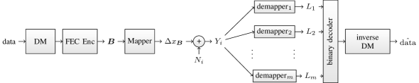
Figure 1: Resulting channel model of the bit-metric decoding receiver structure.

II System Model [4]

We consider transmission over a time discrete AWGN channel

$$Y_{i}=\Delta X_{i}+N_{i}$$ (1)

where the channel input $X_{i}$ has distribution $P_{X}$ on the $2^{m}$- ASK (ASK) constellation $\mathcal{X}=\left\{\pm 1,\pm 3,\ldots,\pm 2^{m}-1\right\}$ and the noise $N_{i}\sim\mathcal{N}(0,1)$ is Gaussian with zero mean and unit variance. We use the constellation scaling $\Delta\in\mathds{R}$ to set the $\text{SNR}=\operatorname{E}\left[(\Delta X_{i})^{2}\right]/1$. Using a uniform distribution on ASK constellations results in a shaping gap of $1.53\text{\,}\mathrm{d}\mathrm{B}$ in the high SNR regime [10, Sec. IV-B] compared to the capacity of the AWGN channel

$$C_{\text{AWGN}}(\text{SNR})=\frac{1}{2}\log_{2}(1+\text{SNR}),$$ (2)

which is achieved with Gaussian inputs of zero mean and variance SNR. This loss can be overcome by employing probabilistic shaping, i.e., imposing a non-uniform distribution on the ASK constellation points [4, Sec. III-D].

II-A Transmitter: Probabilistic Amplitude Shaping

In order to combine probabilistic shaping with FEC, we employ the PAS scheme [4, Sec. IV]. The optimal distribution $P_{X}^{*}$ for the AWGN channel is symmetric around the origin, i.e., $P_{X}^{*}(x)=P_{X}^{*}(-x)$. This allows for factorization into amplitude and sign, i.e.,

$$P_{X}(x)=P_{A}(\left|x\right|)P_{S}(\operatorname*{sign}(x)),$$

where the amplitude $A$ is defined on $\mathcal{A}=\left\{1,3,\ldots,2^{m}-1\right\}$ and $S=\operatorname*{sign}(X)$ is uniformly distributed on $\{-1,+1\}$. For the binary labeling of the constellation points, we use

$$\text{label}(x)=\beta(\operatorname*{sign}(x))\bm{\beta}(\left|x\right|)$$

Herein, the function $\bm{\beta}:\mathcal{A}\to\left\{0,1\right\}^{m-1}$ implements a BRGC (BRGC) [11] and $\beta(-1)=0,\beta(+1)=1$. Assuming a desired FEC blocklength of $n$, a DM (DM) [5] is used to transform uniformly distributed information bits into a sequence of $n_{\text{c}}=n/m$ amplitudes that follow a prescribed distribution and have entropy $\operatorname{H}(A)$. A systematic encoder copies their binary representation $\bm{\beta}(A^{n_{\text{c}}})$ together with potentially $(1-(1-c)\cdot m)\cdot n_{\text{c}}$ other uniformly distributed information bits to the final codeword and appends uniformly distributed check bits. Consequently, we obtain an overall SE $R$ [4, Sec. IV-D] of

$$R=\operatorname{H}(A)+1-(1-c)\cdot m=\operatorname{H}(X)-(1-c)\cdot m.$$ (3)

By changing the distribution $P_{X}$, the SE $R$ can be adjusted seamlessly keeping the same modcod, i.e., the modulation order $2^{m}$ and the code rate $c$.

Remark 1.

In case of uniform inputs, we have $\operatorname{H}(X)=m$, such that (3) reduces to the well known SE $c\cdot m$ of a system with uniform inputs.

II-B Receiver: Bit-Metric Decoding (BMD)

At the receiver side, we use BMD (BMD), i.e., a bitwise demapper followed by a binary decoder. This approach was introduced in [12] and is now mainly known as BICM (BICM) [13]. We identify each constellation symbol by its $m$ bit binary label $\bm{B}=B_{1}B_{2}\ldots B_{m}$, where

$$B_{1} =\beta(\operatorname*{sign}(x)),$$

$$B_{2}B_{3}\ldots B_{m} =\bm{\beta}(\left|x\right|),\quad x\in\mathcal{X}.$$

Bit-metric decoding can be interpreted from a mismatched decoding perspective [14], where the decoder assumes both an auxiliary channel metric $q_{y|\bm{B}}=\prod_{i=1}^{m}p_{Y|B_{i}}(y|b_{i})$ and an auxiliary input distribution $Q_{\bm{B}}(\bm{b})=\prod_{i=1}^{m}P_{B_{i}}(b_{i})$. These assumptions represent a setting with $m$ parallel and independent channels of the form

$$p_{Y|B_{i}}(y|b)=\frac{1}{P_{B_{i}}(b)}\sum_{\xi\in\mathcal{X}^{b}_{i}}p_{Y|X}(y|\xi)P_{X}(\xi),$$

where $\mathcal{X}^{b}_{i}$ denotes the set of symbols $x\in\mathcal{X}$ with $B_{i}=b$. The random variable $B_{i}$ has the marginal distribution

$$P_{B_{i}}(b)=\sum_{\xi\in\mathcal{X}^{b}_{i}}P_{X}(\xi).$$

$P_{B_{i}}(b)$ is both a function of the distribution $P_{X}$ and the labeling. For each bit-level $i=1,\ldots,m$ the soft-demapper then calculates its metric according to

$$L_{i}=\log\left(\frac{P_{B_{i}}(0)}{P_{B_{i}}(1)}\right)+\log\left(\frac{p_{Y|B_{i}}(y|0)}{p_{Y|B_{i}}(y|1)}\right),$$ (4)

which motivates our BICM channel model depicted in Fig. 1.

In [15], a BMD-achievable rate is given by

$$R_{\text{BMD}}=\left[\operatorname{H}(\bm{B})-\sum_{i=1}^{m}\operatorname{H}(B_{i}|Y)\right]^{+},$$ (5)

where $\left[\cdot\right]^{+}=\max(0,\cdot)$.

We introduce the notation $R_{\text{BMD}}(P_{X},\text{SNR})$ to denote the BMD achievable rate with input distribution $P_{X}$ and an average power constraint of SNR. We also introducde $R^{-1}_{\text{BMD}}(P_{X},R)$ which describes the required SNR such that $R_{\text{BMD}}(P_{X},\text{SNR})$ equals $R$.

III Robust LDPC Code Design

We target the design of protograph based LDPC codes that perform well over the range of SE from $0.7\text{\,}\mathrm{bpcu}2.7\text{\,}\mathrm{bpcu}$. We will first show that codes optimized for one specific SE tend to perform bad at other rates. This behavior can be avoided by accounting for the whole range during the code design.

III-A Operating Points and Signaling

We choose our operating points for different SE by changing the entropy of the distribution on the constellation symbols. Following (3) and considering a $c=13/16$ code and a 16-ASK constellation, the entropy and SE are

$$\operatorname{H}(X)=R+\left(1-\frac{13}{16}\right)\cdot 4\quad\Longrightarrow\quad R=\operatorname{H}(X)-\frac{3}{4}.$$ (6)

Let $P_{X}^{R}$ be the MB (MB) distribution [16] that leads to a SE $R$ with a 13/16 rate code.

Remark 2.

By (6) a rate constraint translates into an entropy constraint. The MB distribution is the solution to the following optimization problem:

$$\min_{\text{ \acl{PMF} (\acs{PMF})}P_{X}}\operatorname{E}\left[X^{2}\right]\quad\text{subject to }\quad\operatorname{H}(X)\geq H^{\prime}.$$

Hence, it is a natural choice for power-efficient signaling with an entropy constraint. Note that in general, MB distributions perform well on the AWGN channel, see, e.g., [4, Table I].

Fig. 2 depicts the achievable BMD rate performance for the considered scenario. The points $(\widetilde{\text{SNR}},R)$ on the dashed red curve are given by:

1. Calculate $P_{X}^{R}$ such that $R=\operatorname{H}(X)-\frac{3}{4}\stackrel{{\scriptstyle!}}{{=}}C_{\text{AWGN}}(\text{SNR})$.

2. Calculate $\widetilde{\text{SNR}}$ with $\widetilde{\text{SNR}}=R_{\text{BMD}}^{-1}(P_{X}^{R},R)$.

For reference, we also plot the uniform BMD rate, which is denoted as $R_{\text{BMD}}(P_{U},\text{SNR})$ and $P_{U}(x)=1/16,\forall x\in\mathcal{X}$.

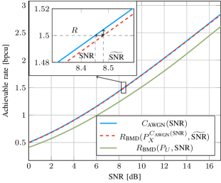
Figure 2: Comparison of $R_{\text{BMD}}$ to $C_{\text{AWGN}}(\text{SNR})$ for uniform and shaped input distributions on 16-ASK.

We observe that the loss due to BMD is negligible. This is also verified in Fig. 3, which depicts the SNR and rate gaps.

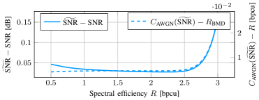
Figure 3: Comparison of the SNR and rate gaps for the considered range of $0.7\text{\,}\mathrm{bpcu}2.7\text{\,}\mathrm{bpcu}$.

III-B Protograph-Based LDPC Code Ensembles

LDPC codes are linear block codes with a sparse $(n-k)\times n$ parity-check matrix $\bm{H}$. The matrix $\bm{H}$ can be represented by a Tanner graph [17, Sec. 3.3] consisting of variable nodes $V_{i},i\in\{1,\ldots,n\}$ and check nodes $C_{j},j\in\{1,\ldots,n-k\}$. A variable or check node has degree $d$ if it is connected to $d$ check or variable nodes, respectively. LDPC code ensembles are usually characterized by the degree profiles of the variable and check nodes. For instance, $\lambda(x)=\sum_{d=1}^{d_{v}}\lambda_{d}x^{d-1}$ and $\rho(x)=\sum_{d=1}^{d_{c}}\rho_{d}x^{d-1}$ are the edge-perspective variable and check node degree polynomials with maximum degree $d_{v}$ and $d_{c}$, respectively. However, the degree profiles can not characterize the mapping of variable nodes to the $m$ different bit-channels resulting from our adapted BICM transmission scheme, see Fig. 1. In the following, we use the structured ensembles of protographs [9] to incorporate the bit-mapping in our threshold analysis. Protographs can be seen as a special instance of multi-edge type LDPC codes [18], where each edge represents an individual edge type.

Parity-check matrices are constructed from protographs as follows. Starting from a small bipartite graph represented via its basematrix $\bm{A}=[a_{lk}]$ of size $M\times N$, where $a_{lk}$ represents the number of edges between the protograph variable node $V_{k},k\in\{1,\ldots,N\}$ and the protograph check node $C_{l},l\in\{1,\ldots,M\}$, one applies a copy-and-permute operation (also known as lifting) to create $Q$ instances of the small graph and then permutes the edges so that the local edge connectivity remains the same. The $Q$ replicas of variable node $V_{k}$ must be connected only to replicas of the neighbors of $V_{k}$ while maintaining the original degrees for that specific edge. The resulting bipartite graph representing the final parity-check matrix $\bm{H}$ possesses $n=Q\cdot N$ variable nodes and $n-k=Q\cdot M$ check nodes. Parallel edges are allowed, but must be resolved during the copy-and-permute procedure.

III-C Code Design for Surrogate Channels

As pointed out in our previous work [8, Sect. IV], the usual design approaches for LDPC codes fail for the BICM channel because they rely on the assumption of binary-input symmetric-output channels so that the transmission of the all-zero codeword can be assumed for the analysis. The BICM channel densities $p_{L_{i}|B_{i}}$ do not exhibit this property, in particular when shaping is taken into account. Instead, [8] pursues an approach based on surrrogate channels, i.e., each BICM channel $p_{L_{i}|B_{i}}$ is replaced by a binary-input symmetric-output AWGN channel $\tilde{L}_{i}=\tilde{B}_{i}+\tilde{N}_{i}$ with $\tilde{B}_{i}$ uniform on $\{\pm\frac{2}{\sigma^{2}_{i}}\}$ and $\tilde{N}_{i}$ zero mean Gaussian with variance $\frac{4}{\sigma_{i}^{2}}$. The parameter $\sigma_{i}^{2}$ is now chosen such that

$$\operatorname{H}(\tilde{B}_{i}|\tilde{L}_{i})\stackrel{{\scriptstyle!}}{{=}}\operatorname{H}(B_{i}|L_{i}),\quad i=1,2,\ldots,m.$$ (7)

Using the surrogates, density evolution or methods based on EXIT (EXIT) charts can readily be applied. For our protograph based design, we resort to the PEXIT approach [19] to determine the asymptotic decoding threshold of a protograph ensemble. In the following, the notion of the asymptotic decoding threshold for $m$ parallel binary input AWGN channels is made precise.

We allow different variable node degrees for each of the $m$ distinct bit-channels. In order to have up to $D$ different degrees per bit-channel, the protograph matrix $\bm{A}$ must have at least $N=D\cdot m$ variable nodes. We introduce a mapping function of the form $T(k)=\left\lceil k/D\right\rceil$ to relate each protograph variable node $V_{k}$ to a corresponding bit-level $T(k)\in\{1,\ldots,m\}$. Let $\bm{\sigma}_{\text{SNR},P_{X}^{R}}=\begin{pmatrix}\sigma_{T(1)},\ldots,\sigma_{T(k)}\end{pmatrix}^{\mathrm{T}}$ be the set of surrogate channel parameters for a specific SNR and SE $R$ and let $I_{\text{app},k}^{\ell}$ be the a-posteriori mutual information of the $k$-th variable node in the $\ell$-th PEXIT iteration. The SNR convergence region $\mathcal{D}(\bm{A},P_{X}^{R})$ of the protograph $\bm{A}$ and using $P_{X}^{R}$ is then given as

$$\mathcal{D}(\bm{A},P_{X}^{R})=\left\{\text{SNR}\left|\bm{\sigma}_{\text{SNR},P_{X}^{R}}:I_{\text{app},k}^{\ell}\xrightarrow{\ell\to\infty}1,\forall k\right.\right\}.$$

The asymptotic decoding threshold follows as

$$\text{SNR}^{\text{th}}(\bm{A},P_{X}^{R})=\min\mathcal{D}(\bm{A},P_{X}^{R}).$$ (8)

III-D Differential Evolution and Optimization Metric

In order to find the protograph ensemble with the best decoding threshold, we employ differential evolution [20]. As the entries $a_{lk}$ of the protograph matrix $\bm{A}$ are integers, the original formulation has to be adopted as shown in [21, 22]. The asymptotic decoding threshold (8) is used as a metric for the selection of new population members, if the code is optimized for a single SE: A member $\bm{A}^{(g-1)}$ of the previous generation $(g-1)$ is replaced by its potential successor $\tilde{\bm{A}}^{(g)}$ if and only if $\tilde{\bm{A}}^{(g)}$ has a smaller asymptotic decoding threshold than $\bm{A}^{(g-1)}$. For the robust design, we advocate for the metric

$$\bm{A}^{(g)}=\operatorname*{argmin}_{\bm{A}\in\{\bm{A}^{(g-1)},\tilde{\bm{A}}^{(g)}\}}\max_{R\in\mathcal{P}}\text{SNR}^{\text{th}}(\bm{A},P_{X}^{R})-R^{-1}_{\text{BMD}}(P_{X}^{R},R),$$ (9)

where $\mathcal{P}\subseteq\left[$0.7$;$2.7$\right]$ is the set of all considered operating points for which the code should be optimized.

IV Simulation Results

We design a rate 13/16 code which allows up to $D=4$ different variable node degrees per bit-level such that the resulting base matrices have dimensions $3\times 16$. The number of parallel edges is limited to 3, which results in a maximum variable node degree of 9. The number of degree 2 variable nodes is limited to one column and all other nodes must have a degree of at least 3 to ensure a linear growth of the minimum distance [23]. We optimize basematrices for five scenarios. The first four target specific SE of $0.7\text{\,}\mathrm{bpcu}$, $1.1\text{\,}\mathrm{bpcu}$, $2.1\text{\,}\mathrm{b}\mathrm{p}\mathrm{c}\mathrm{u}$ and $2.7\text{\,}\mathrm{bpcu}$, respectively. The last protograph $\bm{A}_{\text{rob}}$ represents the robust approach that targets all rates in the interval $\left[0.7;2.7\right]$ jointly and is given as

$$\setcounter{MaxMatrixCols}{16}\begin{pmatrix}3&1&1&2&1&2&2&1&0&1&1&1&3&1&1&1\\ 3&2&2&0&2&2&2&2&2&0&1&1&3&2&1&2\\ \makebox[0.0pt][l]{$\smash{\underbrace{\phantom{\begin{matrix}3&0&0&1\end{matrix}}}_{\text{$B_{2}$}}}$}3&0&0&1&\makebox[0.0pt][l]{$\smash{\underbrace{\phantom{\begin{matrix}0&0&0&0\end{matrix}}}_{\text{$B_{3}$}}}$}0&0&0&0&\makebox[0.0pt][l]{$\smash{\underbrace{\phantom{\begin{matrix}1&2&3&3\end{matrix}}}_{\text{$B_{4}$}}}$}1&2&3&3&\makebox[0.0pt][l]{$\smash{\underbrace{\phantom{\begin{matrix}3&0&0&0\end{matrix}}}_{\text{$B_{1}$}}}$}3&0&0&0\end{pmatrix}$$

For its optimization, we chose $\mathcal{P}=\left\{0.7,1.1,2.1,2.7\right\}$. Including further rates did not improve the asymptotic decoding thresholds considerably – using less or other operating points resulted in inferior performance. We observed good results by including the boundaries of the operating region and pursuing the following heuristic approach: For each SE $R$ consider the set of surrogate channel parameters $\bm{\sigma}_{\text{SNR},P_{X}^{R}}$, which exhibit a certain ordering (“quality”) of the individual $m$ bit channels. If this ordering changes at a certain SE $R$ compared to previous ones, $R$ should be added to $\mathcal{P}$. In the considered example, the ordering of $\sigma_{1}$ and $\sigma_{4}$ changes around $R\approx$1.1\text{\,}\mathrm{bpcu}$$ and again $\sigma_{1}$ and $\sigma_{3}$ at around $R\approx$2.1\text{\,}\mathrm{bpcu}$$. For small protograph sizes and limited degrees of freedom, it may suffice to consider the boundary operating points only.

The protographs $\bm{A}_{R},R\in\{0.7,1.1,2.1,2.7\}$ as well as their parity-check-matrices can be found online at [24].

Fig. 4 depicts the SNR gap of the asymptotic decoding thresholds to AWGN capacity, i.e., $\text{SNR}^{\text{th}}(\bm{A},P_{X}^{R})-(2^{2R}-1)$, in $\mathrm{d}\mathrm{B}$ for the considered range of SE. Protographs which are optimized for one particular SE tend to perform poor if operated at other SE. This is particularly the case for the codes optimized for high SE, where the gap increases up to $1.3\text{\,}\mathrm{d}\mathrm{B}$ when operated at lower SNR. The robust protograph design exhibits the desired feature of minimizing the maximum gap for each operating point in $\mathcal{P}$ and therefore achieves a balanced behavior.

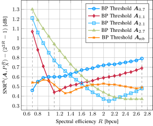
Figure 4: Gap in $\mathrm{d}\mathrm{B}$ to $C_{\text{AWGN}}(\text{SNR})$ of the asymptotic protograph BP decoding thresholds (8) over the range of considered spectral efficiencies.

For a finite length comparison in Fig. 5, the protographs have first been lifted by a factor of three to remove parallel edges and then by a factor of $338$ to yield parity-check matrices of size $2705\times 16224$. As a baseline for performance comparison, we choose the 5/6 DVB-S2 code for short frame sizes, which has a blocklength of $n=16200$ [3]. For the bit-mapping, bit-levels two to four are assigned consecutively to the first 12150 variable nodes, whereas bit-level one is assigned to the remaining ones. As the information part of the parity-check matrix has mostly degree three variable nodes and only a small number of 360 degree 13 variable nodes, optimizing the bit-mapper did not improve performance. In addition to the DVB-S2 reference, we also plot the random coding bound $2^{-n_{\text{c}}E_{G}(R)}$ [25], which provides an upper bound on the frame error performance of a random code ensemble for a given blocklength. Hereby, $E_{G}(R)$ denotes the Gallager exponent for rate $R$.

In all cases, $100$ BP iterations with a full sum-product update rule are performed. We observe that the predictions of the asymptotic decoding thresholds are well reflected in the finite-length performance as well.

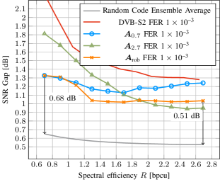
Figure 5: Gap in $\mathrm{d}\mathrm{B}$ to $C_{\text{AWGN}}(\text{SNR})$ for different protograph designs over the range of considered spectral efficiencies at a target FER of ${10}^{-3}$.

V Conclusion

In this work, we proposed a novel, robust design approach for protograph based LDPC codes for rate-adaptive communication via probabilistic amplitude shaping. Using one 16-ASK constellation and one 13/16 rate code, any SE between $0.7\text{\,}\mathrm{bpcu}2.7\text{\,}\mathrm{bpcu}$ can be achieved with a gap of at most $1.3\text{\,}\mathrm{d}\mathrm{B}$ for a target FER of ${10}^{-3}$ and a blocklength of $16\,224$. Future research should focus on investigating other robust optimization metrics, such as the rate-backoff at the decoding threshold and the influence of the choice of operating points in the set $\mathcal{P}$.

References

- [1] LTE; Evolved Universal Terrestrial Radio Access (E-UTRA); Physical layer procedures, European Telecommun. Standards Inst. (ETSI) Std. TS 136 213, Rev. 11.2.0, 2013.
- [2] Digital Video Broadcasting (DVB); Second generation framing structure, channel coding and modulation systems for Broadcasting, Interactive Services, News Gathering and other broadband satellite applications; Part 2: DVB-S2 Extensions (DVB-S2X), European Telecommun. Standards Inst. (ETSI) Std. EN 302 307-2, Rev. 1.1.1, 2014.
- [3] Digital Video Broadcasting (DVB); 2nd Generation Framing Structure, Channel Coding and Modulation Systems for Broadcasting, Interactive Services, News Gathering and Other Broadband Satellite Applications (DVB-S2), European Telecommun. Standards Inst. (ETSI) Std. EN 302 307, Rev. 1.2.1, 2009.
- [4] G. Böcherer, F. Steiner, and P. Schulte, “Bandwidth Efficient and Rate-Matched Low-Density Parity-Check Coded Modulation,” IEEE Trans. Commun., vol. 63, no. 12, pp. 4651–4665, Dec. 2015.
- [5] P. Schulte and G. Böcherer, “Constant Composition Distribution Matching,” IEEE Trans. Inf. Theory, vol. 62, no. 1, pp. 430–434, Jan. 2016.
- [6] F. Buchali, G. Böcherer, W. Idler, L. Schmalen, P. Schulte, and F. Steiner, “Experimental demonstration of capacity increase and rate-adaptation by probabilistically shaped 64-QAM,” in 2015 European Conference on Optical Communication (ECOC), Sep. 2015, paper PDP3.4.
- [7] F. Buchali, F. Steiner, G. Böcherer, L. Schmalen, P. Schulte, and W. Idler, “Rate Adaptation and Reach Increase by Probabilistically Shaped 64-QAM: An Experimental Demonstration,” J. Lightw. Technol., vol. 34, no. 7, pp. 1599–1609, Apr. 2016.
- [8] F. Steiner, G. Böcherer, and G. Liva, “Protograph-Based LDPC Code Design for Shaped Bit-Metric Decoding,” IEEE J. Sel. Areas Commun., vol. 34, no. 2, pp. 397–407, Feb. 2016.
- [9] J. Thorpe, “Low-density parity-check (LDPC) codes constructed from protographs,” IPN progress report, vol. 42, no. 154, pp. 42–154, 2003.
- [10] G. Forney, R. Gallager, G. Lang, F. Longstaff, and S. Qureshi, “Efficient Modulation for Band-Limited Channels,” IEEE J. Sel. Areas Commun., vol. 2, no. 5, pp. 632–647, Sep. 1984.
- [11] F. Gray, “Pulse code communication,” U. S. Patent 2 632 058, 1953.
- [12] E. Zehavi, “8-PSK trellis codes for a Rayleigh channel,” IEEE Trans. Commun., vol. 40, no. 5, pp. 873–884, May 1992.
- [13] G. Caire, G. Taricco, and E. Biglieri, “Bit-interleaved coded modulation,” IEEE Trans. Inf. Theory, vol. 44, no. 3, pp. 927–946, May 1998.
- [14] A. Martinez, A. Guillen i Fabregas, G. Caire, and F. Willems, “Bit-Interleaved Coded Modulation Revisited: A Mismatched Decoding Perspective,” IEEE Trans. Inf. Theory, vol. 55, no. 6, pp. 2756–2765, Jun. 2009.
- [15] G. Böcherer, “Achievable rates for shaped bit-metric decoding,” arXiv preprint, 2016. [Online]. Available: http://arxiv.org/abs/1410.8075
- [16] F. Kschischang and S. Pasupathy, “Optimal nonuniform signaling for Gaussian channels,” IEEE Trans. Inf. Theory, vol. 39, no. 3, pp. 913–929, May 1993.
- [17] T. Richardson and R. Urbanke, Modern coding theory. Cambridge University Press, 2008.
- [18] ——, “Multi-edge type LDPC codes,” Workshop honoring Prof. Bob McEliece on his 60th birthday, California Institute of Technology, Pasadena, California, pp. 24–25, 2002.
- [19] G. Liva and M. Chiani, “Protograph LDPC Codes Design Based on EXIT Analysis,” in Proc. IEEE Global Telecommun. Conf. (GLOBECOM), Nov. 2007, pp. 3250–3254.
- [20] R. Storn and K. Price, “Differential Evolution – A Simple and Efficient Heuristic for Global Optimization over Continuous Spaces,” J. Global Optimization, vol. 11, no. 4, pp. 341–359, Dec. 1997.
- [21] A. Pradhan, A. Subramanian, and A. Thangaraj, “Deterministic constructions for large girth protograph LDPC codes,” in Proc. IEEE Int. Symp. Inf. Theory (ISIT), Jul. 2013, pp. 1680–1684.
- [22] H. Uchikawa, “Design of non-precoded protograph-based LDPC codes,” in Proc. IEEE Int. Symp. Inf. Theory (ISIT), Jun. 2014, pp. 2779–2783.
- [23] T. V. Nguyen, A. Nosratinia, and D. Divsalar, “The Design of Rate-Compatible Protograph LDPC Codes,” IEEE Trans. Commun., vol. 60, no. 10, pp. 2841–2850, Oct. 2012.
- [24] Protograph and parity-check matrices of the considered example. [Online]. Available: http://experimental-it.org/istc2016/
- [25] R. G. Gallager, Information Theory and Reliable Communication. John Wiley & Sons, Inc., 1968.