Detection of Solar-Like Oscillations, Observational Constraints, and Stellar Models for $\theta$ Cyg, the Brightest Star Observed by the Kepler Mission

Abstract

$\theta$ Cygni is an F3 spectral-type main-sequence star with visual magnitude V=4.48. This star was the brightest star observed by the original Kepler spacecraft mission. Short-cadence (58.8 s) photometric data using a custom aperture were obtained during Quarter 6 (June-September 2010) and subsequently in Quarters 8 and 12-17. We present analyses of the solar-like oscillations based on Q6 and Q8 data, identifying angular degree $l$ = 0, 1, and 2 oscillations in the range 1000-2700 $\mu$Hz, with a large frequency separation of 83.9 $\pm$ 0.4 $\mu$Hz, and frequency with maximum amplitude $\nu_{\rm max}$ = 1829 $\pm$ 54 $\mu$Hz. We also present analyses of new ground-based spectroscopic observations, which, when combined with angular diameter measurements from interferometry and Hipparcos parallax, give $T_{\mathrm{eff}}$ = 6697 $\pm$ 78 K, radius 1.49 $\pm$ 0.03 R_⊙, [Fe/H] = -0.02 $\pm$ 0.06 dex, log $g$ = 4.23 $\pm$ 0.03. We calculate stellar models matching the constraints using several methods, including using the Yale Rotating Evolution Code and the Asteroseismic Modeling Portal. The best-fit models have masses 1.35–1.39 M_⊙ and ages 1.0–1.6 Gyr. $\theta$ Cyg’s $T_{\mathrm{eff}}$ and log $g$ place it cooler than the red edge of the $\gamma$ Doradus instability region established from pre-Kepler ground-based observations, but just at the red edge derived from pulsation modeling. The best-fitting models have envelope convection-zone base temperature of $\sim$320,000 to 395,000 K. The pulsation models show $\gamma$ Dor gravity-mode pulsations driven by the convective-blocking mechanism, with periods of 0.3 to 1 day (frequencies 11 to 33 $\mu$Hz). However, gravity modes were not detected in the Kepler data; one signal at 1.776 c d^-1 (20.56 $\mu$Hz) may be attributable to a faint, possibly background, binary. Asteroseismic studies of $\theta$ Cyg, in conjunction with those for other A-F stars observed by Kepler and CoRoT, will help to improve stellar model physics to sort out the confusing relationship between $\delta$ Sct and $\gamma$ Dor pulsations and their hybrids, and to test pulsation driving mechanisms.

1 Introduction

The mission of the NASA Kepler spacecraft, launched 2009 March 7, was to search for Earth-sized planets around Sun-like stars in a fixed field of view in the Cygnus-Lyra region using high-precision CCD photometry to detect planetary transits (Borucki et al., 2010). As a secondary mission Kepler surveyed and monitored over 10,000 stars for asteroseismology, using the intrinsic brightness variations caused by pulsations to infer the star’s mass, age, and interior structure (Gilliland et al., 2010a). After the failure of the second of four reaction wheels, the Kepler mission transitioned into a new phase, K2 (Howell et al., 2014), observing fields near the ecliptic plane for about 90 days each, with a variety of science objectives including planet searches.

The $V\,=\,4.48$ F3 spectral-type main-sequence star $\theta$ Cyg, also known as 13 Cyg, HR 7469, HD 185395, 2MASS 19362654+5013155, HIP 96441, and KIC 11918630, where KIC = Kepler Input Catalog (Brown et al., 2011), is the brightest star that fell on active pixels in the original Kepler field of view. $\theta$ Cyg is nearby and bright, so that high-precision ground-based data can be combined with high signal-to-noise and long time-series Kepler photometry to provide constraints for asteroseismology. The position of $\theta$ Cyg in the HR diagram is near that of known $\gamma$ Dor pulsators, suggesting the possibility that it may exhibit high-order gravity mode pulsations, which would probe the stellar interior just outside its convective core. $\theta$ Cyg is also cool enough to exhibit solar-like $p$-mode (acoustic) oscillations, which probe both the interior and envelope structure.

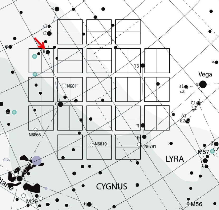
Figure 1: Kepler field of view with stars marked according to stellar magnitude created using “The Sky” astronomy software (http://www.bisque.com/sc/pages/TheSkyX-Editions.aspx). The location of $\theta$ Cyg is shown by the red arrow, and is marked with the symbol $\theta$ and a filled circle designating magnitude 4-5. Note that all stars brighter than $\theta$ Cyg fall in the regions between the CCD arrays to avoid saturating pixels.

$\theta$ Cyg has been observed using adaptive optics (Desort et al., 2009). It has a resolved binary M-dwarf companion of $\sim$0.35 M_⊙ with separation 46 AU. Following the orbit for nearly an orbital period (unfortunately $\sim$ 230 y) will eventually give an accurate dynamical mass for $\theta$ Cyg. Also, the system shows a 150-d quasi-period in radial velocity, suggesting that one or more planets could accompany the stars (Desort et al., 2009).

$\theta$ Cyg has also been observed using optical interferometry (Ligi et al., 2012; Boyajian et al., 2012; White et al., 2013, see Section 4). These observations provide tight constraints on the radius of $\theta$ Cyg and therefore a very useful constraint for asteroseismology.

$\theta$ Cyg’s projected rotational velocity is low; $v~{}\sin i$ = $3.4\pm 0.4$  km s^-1 (Gray, 1984, see Section 3). If $\sin i$ is not too small, $\theta$ Cyg’s slow rotation should simplify mode identification and pulsation modeling, as spherical approximations and low-order perturbation theory for the rotational splitting should be adequate.

This paper is intended to provide background on the $\theta$ Cyg system and to be a first look at the Kepler photometry data and consequences for stellar models and asteroseismology. We present light curves and detection of the solar-like $p$-modes based on Kepler data taken in observing Quarters 6 and 8 (Section 2). We summarize ground-based observational constraints from the literature (Appendix A) and present analyses based on new spectroscopic observations (Section 3) and optical interferometry (Section 4). We discuss inference of stellar parameters based on the large separation and frequency of maximum amplitude (Section 5), line widths (Section 6), and mode identification (Section 7). We use the observed $p$-mode oscillation frequencies and mode identifications as constraints for stellar models using several methods (Section 8). We discuss predictions for $\gamma$ Dor $g$-mode pulsations (Section 9), and results of a search for low frequencies consistent with $g$ modes (Section 10). We conclude with motivation for continued study of $\theta$ Cyg (Section 11).

We do not include in this paper the analyses of data from Quarters 12-17 for several reasons. First, we completed the bulk of this paper, including the spectroscopic analyses, and first asteroseismic analyses at the time when only the Q6 and Q8 data were available. Second, a problem has emerged with the Kepler data reduction pipeline for the latest data release for short-cadence data that will not be corrected until later in 2016; while $\theta$ Cyg is not on the list of affected stars, because $\theta$ Cyg required so many pixels and special processing, more work is needed to confirm that the problem has not introduced additional noise in the light curve. We estimate that inclusion of the full time-series data will result in finding a few more frequencies, and will improve the precision of the frequencies obtained by a factor of $\sim$1.8. Comparison of studies of the bright (V = 5.98) Kepler targets 16 Cyg A and B using one month versus thirty months of data show that the longer time series improved the accuracy and precision of results, but did not significantly change the frequencies or inferred stellar model parameters (Metcalfe et al., 2012, 2015).

Detailed analyses making use of the remaining time-series data and the Kepler pixel data will be the subject of future papers.

2 Detection of $\theta$ Cyg Solar-Like Oscillations by Kepler

$\theta$ Cyg is seven magnitudes brighter than the saturation limit of the Kepler photometry. Figure 1 shows the Kepler field of view superimposed on the constellations Cygnus and Lyra with $\theta$ Cyg on the CCD module at the top of the leftmost column in this figure. Kepler stars are observed using masks that define the pixels to be stored for that star. Special apertures can be defined to better conform to the distribution of charge for extremely saturated targets (see, e.g., Kolenberg et al., 2011). For $\theta$ Cyg the number of recorded pixels required was reduced from $>$10,000 to $\sim$1,800 by using an improved special aperture.

$\theta$ Cyg was observed 2010 June$-$September (Kepler Quarter 6) and 2011 Jan$-$March (Quarter 8) in short cadence (58.8 s integration; see Gilliland et al. (2010b) for details). Kepler measurements were organized in quarters because the satellite performed a roll every three months to maintain the solar panels directed towards the Sun and the radiators to cool the focal plane in shadow. Moreover, every month the satellite stopped data acquisition for less than 24 hours and pointed towards the Earth to transmit the stored data. Therefore, monthly interruptions occured in the Kepler observations. More details on the Kepler window function can be found in García et al. (2014a).

Figure 2 shows the 90-day minimally processed short-cadence light curves for Q6 and Q8. $\theta$ Cyg was not well-captured by the dedicated mask for $\sim$50% of Quarter 6 (a problem resolved for observations in subsequent quarters), so 42 d of the best-quality data in the flat portion of the Q6 light curve were used in the pulsation analysis. During Q8, the spacecraft entered a safe mode Dec. 22-Jan. 6, causing data loss at the beginning of the quarter, so only 67 d of data were obtained.

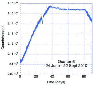
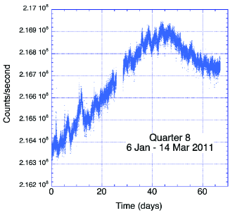
Figure 2: Kepler $\theta$ Cyg unprocessed light curve for Quarter 6 (left) and Quarter 8 (right). The custom aperture captured the target completely in Q6 only during 42 d (flat portion of curve) used in this analysis. The spacecraft entered a safe mode for part of Q8, so only 67 days of data were obtained.

These light curves were processed following the methods described by García et al. (2011) to remove outliers, jumps and drifts, as was done for other solar-like stars (e.g. Campante et al., 2011; Mathur et al., 2011a; Appourchaux et al., 2012b), including the binary system 16 Cyg (Metcalfe et al., 2012), where a special treatment was also applied because it is composed of two very bright stars. For the solar-like oscillation analysis of $\theta$ Cyg, we have removed the drifts by using a triangular smoothing filter with a width of 10 days (frequency 1.16 $\mu$Hz). The triangular smoothing filter is a rectangular (box car) filter of 10 days applied twice to the data; hence it is the convolution of two box cars, which is a triangle. Figure 3 shows the resultant light curve for the Q6 and Q8 data.

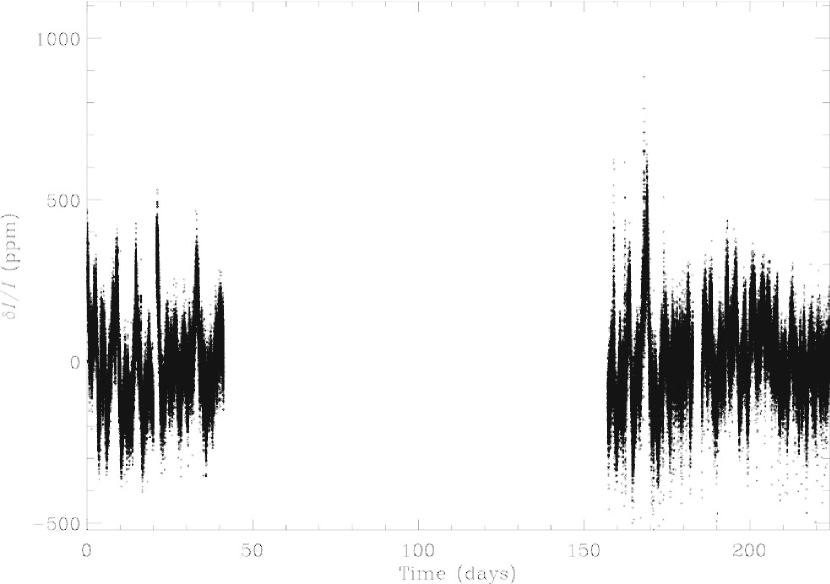
Figure 3: Combined Q6 and Q8 light curve after detrending and applying a 10-day triangular filter to remove low-frequency variations.

The Fourier Transform of the Q6 data revealed a rich spectrum of overtones of solar-like oscillations, with excess power above the background in the frequency range $\sim$1200 to 2500 $\mu$Hz. Figure 4 shows the power-density spectrum of the processed Q6 and Q8 data. The data show a large frequency separation $\Delta$$\nu$ of $\sim$84 $\mu$Hz with maximum oscillation amplitude at $\nu_{\rm max}$ = 1830 $\mu$Hz. The appearance of the oscillation spectrum is very similar to that of other well-studied F stars such as Procyon A (Bedding et al., 2010b; Bond et al., 2015), HD49933 (Appourchaux et al., 2008; Benomar et al., 2009b; Reese et al., 2012), HD181420 (Barban et al., 2009), and HD181906 (García et al., 2009); see also Table 1 of Mosser et al. (2013) and references therein. The envelope of oscillation power is very wide, and modes are evidently heavily damped, meaning the resonant peaks have large widths in the frequency spectrum, which makes mode identification difficult (see, e.g., Bedding & Kjeldsen, 2010a, and discussion in Section 7). For comparison to $\theta$ Cyg’s $\nu_{\rm max}$ (1830 $\mu$Hz), the maximum in the Sun’s power spectrum is at about 3150 $\mu$Hz, while for Procyon with mass 1.48 M_⊙ and luminosity 6.93 L_⊙, $\nu_{\rm max}$ is 1014 $\mu$Hz (Huber et al., 2011), and for HD49933, with mass 1.30 M_⊙ and luminosity 3.47 L_⊙, $\nu_{\rm max}$ is 1760 $\mu$Hz (Appourchaux et al., 2008).

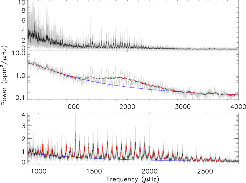
Figure 4: Top: Power-density spectrum of the Q6 and Q8 data shown using the minimally processed data (grey) and using a box-car smoothing of width $3$ $\mu$Hz (black). Middle: Power spectrum with a smoothing of width $3$ $\mu$Hz (grey) or $\Delta\nu/2=42$ $\mu$Hz (black). Superimposed is shown the best fit of the mode envelope with a Gaussian (red) and of the noise background (blue). Bottom: Zoom-in on the modes. The power spectrum is smoothed over $0.5$ $\mu$Hz (grey) or $3$ $\mu$Hz (black). The red curve shows the best fit to the individual pulsation modes with Lorentzian profiles.

3 New High-Resolution Spectra and Analyses

A review of the extensive literature prior to the Kepler observations suggests that $\theta$ Cyg is a normal, slowly rotating, solar-composition, F3V spectral-type star (Gray et al., 2003) with $T_{\mathrm{eff}}$ around 6700$\pm$100 K and $\log g$ around 4.3$\pm$0.1 dex (see Appendix A). This section summarizes analyses of high-resolution spectra taken subsequent to the Kepler observations by P. I. Pápics at the HERMES spectrograph on the Mercator Telescope in May 2011, and by the team of D. Latham at the TRES spectrograph in December 2011.

3.1 HERMES spectrum analyses of $\theta$ Cygni

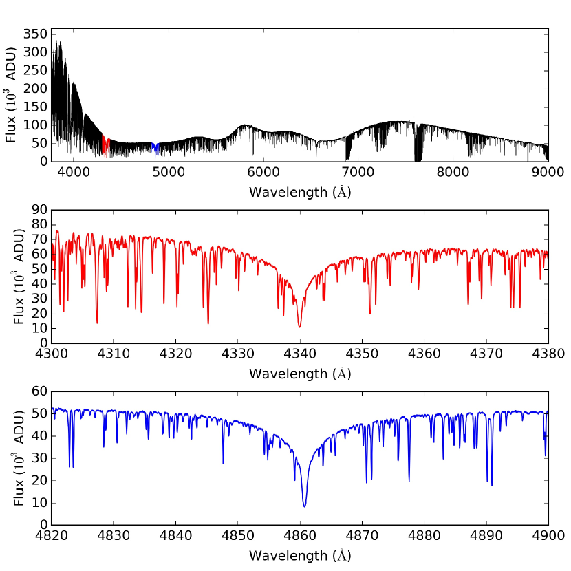
Figure 5: High-resolution spectrum of $\theta$ Cyg taken with HERMES Mercator spectrograph in May 2011 (top), and region around H$\gamma$ (middle) and H$\beta$ (bottom).

High-resolution high signal-to-noise spectra were taken using the HERMES spectrograph (Raskin et al., 2011) installed on the 1.2-meter Mercator telescope based at the Roque de los Muchachos Observatory on La Palma, Canary Islands, Spain. The spectrograph is bench-mounted and fiber-fed, and resides in a temperature-controlled enclosure to guarantee instrumental stability. During the observations, HERMES was set to the HRF mode using the high-resolution fiber with a spectral resolving power of $R=85,000$ delivering a spectral coverage from 377 to 900 nm in a single exposure and a peak efficiency of 28%. The final processed orders, along with merged spectra, were obtained on site using the integrated HERMES data reduction pipeline.

Analyses of the HERMES spectrum (Fig. 5), discussed next, was undertaken independently by five of us, using differing methods.

3.1.1 vwa

The Versatile Wavelength Analysis (vwa) method uses spectral synthesis to fit lines to determine their equivalent widths (EWs). $T_{\rm eff}$ is found by adjusting it to remove any slope in the Fe i versus excitation potential of the lower level, using lines with EW$<$100mÅ. The criterion for $\log{g}$ is that the average abundance from the Fe i and Fe ii lines agree. In addition, checks are made that Mg i b and Ca lines at 6122Å and 6162Å are well fitted. Since Van der Waals broadening is important for these lines, they have been adjusted to agree with the solar spectrum for $\log{g}$ = 4.437 (Bruntt et al., 2010b). The Fe abundance relative to solar, [Fe/H], is calculated as the mean of Fe i lines with EW$<$100 mÅ and $>$5 mÅ. Microturbulence, ${v_{\rm mic}}$, is found by minimizing Fe i abundances versus EW, using only lines with EW$<$90 mÅ. Model atmospheres are an interpolation in the MARCS grid, with line lists from VALD (Kupka et al., 1999). Using a solar spectrum, each line has been forced to give the abundance in Grevesse et al. (2007), in order to give the correction to the $\log{gf}$ values. Non-LTE effects are considered using Rentzsch-Holm (1996), since these effects can be important for stars with $T_{\rm eff}$ above 6500 K.

3.1.2 uclsyn

The analysis was performed based on the methods given in Doyle et al. (2013). The uclsyn code (Smith & Dworetsky, 1988; Smith, 1992) was used to perform the analysis and Kurucz atlas9 models with no overshooting were used (Castelli et al., 1997). The line list was compiled using the VALD database. The $H\alpha$ and $H\beta$ lines were used to give an initial estimate of $T_{\rm eff}$. The $\log{g}$ was determined from the Ca i line at 6439Å, along with the Na i D lines. Additional $T_{\rm eff}$ and $\log{g}$ diagnostics were performed using the Fe lines; however, the $T_{\rm eff}$ acquired from the excitation balance of the Fe i lines was found to be too high ($\sim$ 6900 K) and this $T_{\rm eff}$ was not used. A null dependence between the abundance and the equivalent width was used to constrain the microturbulence. The $\log{g}$ from the Fe lines was determined by requiring that the Fe i and Fe ii abundances agree, and the $T_{\rm eff}$ was also determined from the ionization balance.

The quoted error estimates include that given by the uncertainties in $T_{\rm eff}$, $\log{g}$, and $v_{\rm mic}$, as well as the scatter due to measurement and atomic data uncertainties.

The projected stellar rotation velocity ($v\sin i$) was determined by fitting the profiles of several unblended Fe i lines in the wavelength range 6000–6200Å. A value for macroturbulence of 6 km s^-1 was assumed, based on slight extrapolations of the calibration by Bruntt et al. (2010a) and Doyle et al. (2014), and a best-fitting value of $v\sin i=4.0\pm 0.4$ km s^-1 was obtained.

3.1.3 rotfit

The rotfit method is based on a $\chi^{2}$ minimization with a grid of spectra of real stars with well-known astrophysical parameters (Frasca et al., 2006; Metcalfe et al., 2010; Molenda-Żakowicz et al., 2013). Thus, full spectral regions (discarding those ones heavily affected by telluric lines), not individual lines, are used. The method derives $T_{\rm eff}$, $\log{g}$, [Fe/H], $v\sin i$ and MK classification.

3.1.4 SynthV

Stellar parameters ($T_{\rm eff}$, $\log{g}$, [M/H], $v_{\rm mic}$ and $v\sin i$) are obtained by computing synthetic spectra and comparing them to the observed spectrum (Lehmann et al., 2011). Atmosphere models were calculated with LLmodels (Shulyak et al., 2004), the computation of synthetic spectra was performed using SynthV (Tsymbal, 1996). Atomic data were taken from VALD. The spectrum synthesis was done on the wavelength range 4047–6849 Å, covering both metal and the first four lines of the Balmer series. The local continuum of the observed spectrum was corrected to fit those of the synthetic ones. $\chi^{2}$ statistics were used to determine the optimum values of the atmospheric parameters and their errors based on the 1-$\sigma$ confidence space in all parameters.

3.1.5 ares + moog

The stellar parameters were obtained from the automatic measurement of the equivalent widths of Fe i and Fe ii lines with ares (Sousa et al., 2007) and then imposing excitation and ionization equilibrium using the moog LTE line analysis code (Sneden, 1973) and a grid of Kurucz atlas9 model atmospheres (Kurucz, 1993). The Fe i and Fe ii line list comprises more than 300 lines that were individually tested using high-resolution spectra to check its stability to automatic measurement with ares. The atomic data were obtained from VALD, but with $\log{gf}$ adjusted through an inverse analysis of the Solar spectrum, in order to allow for differential abundance analyses relative to the Sun (Sousa et al., 2008). The errors on the stellar parameters are obtained by quadratically adding 100 K, 0.13 and 0.06 dex to the internal errors on $T_{\rm eff}$, $\log{g}$ and [Fe/H], respectively. These values were obtained by considering the typical dispersion plotted in each comparison of parameters presented in Sousa et al. (2008). A more detailed discussion on the errors derived for this spectroscopic method can be found in Sousa et al. (2011).

3.2 TRES Spectrum Analysis

Two spectra were obtained with the Tillinghast Reflector Échelle Spectrograph (TRES) on the 1.5-m Tillinghast Reflector at the Smithsonian’s Fred L. Whipple Observatory on Mount Hopkins, Arizona. The resolving power of these spectra is 44,000, and the signal-to-noise ratio per resolution element is 280 and 351 for one-minute exposures on BJD 2455905.568 and 2455906.544, respectively. The wavelength coverage extends from 385 to 909 nm, but only the three orders from 506 to 531 nm were used for the analysis of the stellar parameters using Stellar Parameter Classification (SPC, Buchhave et al., 2012), a tool for comparing an observed spectrum with a library of synthetic spectra. spc is designed to solve simultaneously for $T_{\rm eff}$, [M/H], $\log{g}$ and $v\sin{i}$. In essence, spc cross-correlates an observed spectrum with a library of synthetic spectra for a grid of Kurucz model atmospheres and finds the stellar parameters by determining the extreme of a multi-dimensional surface fit to the peak correlation values from the grid.

The consistency between the spc results for the two observations was excellent, but undoubtedly the systematic errors are much larger, such as the systematic errors due to the library of synthetic spectra. Based on past experience, we assign floor errors of 50 K, 0.1 dex, 0.08 dex and 0.5 km s^-1 for $T_{\rm eff}$, $\log{g}$, [M/H] and $v\sin{i}$, respectively. The library spectra were calculated assuming $v_{\rm mic}$ = 2 km s^-1. In tests of spc it has been noticed that the $\log{g}$ values can disagree systematically with cases that have independent dynamical determinations of the gravity for effective temperatures near 6500 K and above (e.g., for Procyon and Sirius). Therefore, as discussed in the next section, we have also used spc to determine $T_{\rm eff}$ and [M/H] whilst fixing $\log{g}$ to the value obtained from asteroseismology.

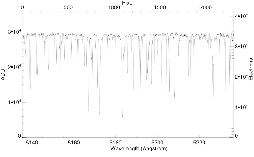
Figure 6: A spectrum of $\theta$ Cyg in the order containing the Mg b triplet, obtained with the TRES spectrograph on the 1.5-m reflector at the Fred Lawrence Whipple Observatory on Mount Hopkins, Arizona. The resolving power is 44,000 and the SNR is 350 per resolution element of 6.8 km/s, at the center of the order. The exposure time was 60 seconds. The échelle blaze function has been removed by dividing with an exposure of a quartz iodine tungsten filament lamp.

Table 1: Summary of the results from the spectral analyses

	vwa	uclsyn	rotfit	SynthV	ares + moog	spc
$T_{\rm eff}$ (K)	6650 $\pm$ 80	6800 $\pm$ 108	6500 $\pm$ 150	6720 $\pm$ 70	6942 $\pm$ 106	6637 $\pm$ 50
$\log{g}$	4.22 $\pm$ 0.08	4.35 $\pm$ 0.08	4.00 $\pm$ 0.15	4.28 $\pm$ 0.19	4.58 $\pm$ 0.14	4.11 $\pm$ 0.1
[Fe/H]	$-$0.07 $\pm$ 0.07	+0.02 $\pm$ 0.08	$-$0.2 $\pm$ 0.1	$-$0.22 $\pm$ 0.05	0.08 $\pm$ 0.06	$-$0.07 $\pm$ 0.08
$v_{\rm mic}$ (km s-1)	1.66 $\pm$ 0.06	1.48 $\pm$ 0.08	n/a	1.93 $\pm$ 0.25	1.94 $\pm$ 0.10	(2.0) ${\dagger}$
$v\sin{i}$ (km s-1)	n/a	4.0 $\pm$ 0.4	4.0 $\pm$ 1.5	6.36 $\pm$ 0.61	n/a	7.0 $\pm$ 0.5
fixing $\log{g}=4.23\pm 0.03$
$T_{\rm eff}$ (K)	6650 $\pm$ 80	6715 $\pm$ 92	n/a	6716 $\pm$ 67	6866 $\pm$ 125	6705 $\pm$ 50
[Fe/H]	$-$0.07 $\pm$ 0.07	$-$0.03 $\pm$ 0.09	n/a	$-$0.21 $\pm$ 0.05	0.06 $\pm$ 0.06	$-$0.03 $\pm$ 0.08
$v_{\rm mic}$ (km s-1)	1.66 $\pm$ 0.06	1.48 $\pm$ 0.08	n/a	1.92 $\pm$ 0.24	1.89 $\pm$ 0.10	(2.0) ${\dagger}$

3.3 Stellar Parameters

A summary of the results from the spectral analyses is given in Table 1. There is a relatively large spread in the values of $T_{\rm eff}$ and $\log{g}$ obtained from the spectral analyses. Examination of their locations in the $T_{\rm eff}$–$\log{g}$ diagram (Fig. 7), shows an apparent correlation between these two parameters. This coupling between the two parameters is a known and common problem with spectral analyses, with some methods more susceptible than others.

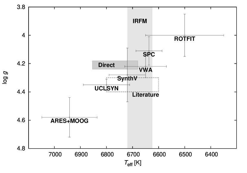
Figure 7: Comparisons of results from the analyses of HERMES and TRES spectra. The range of values of $T_{\rm eff}$ obtained by Blackwell & Lynas-Gray (1998) using the IRFM is shown by the light grey band. The interferometric $T_{\rm eff}$ from Ligi et al. (2012) and the asteroseismic $\log{g}$ value are given as the dark grey box labelled ‘Direct’. The dashed box indicates the most-probable parameters from the literature review.

To address this degeneracy, the spectral analyses were, therefore, repeated using a fixed $\log{g}=4.23\pm 0.03$ derived from the interferometric and asteroseismic constraints on $\theta$ Cyg’s mass and radius from White et al. (2013), and which is also in line with the log $g$ values of the best-fit asteroseismic models discussed in Section 8. The exception is rotfit, which due to its design for use with a grid of real stars, cannot be used to derive parameters for a fixed $\log{g}$. The results from the other methods are presented in the lower part of Table 1. With the exception of ares + moog, the model-atmosphere spectroscopic methods all agree to within the error bars and differ by less than 70 K. The ares + moog method is differential to the Sun, with a line list specifically prepared for precise analysis of stars with temperatures closer to solar, and, therefore, $\theta$ Cyg is too hot for this differential analysis.

It is interesting to explore why the model-independent rotfit method is giving slightly lower values. Fitting a spectrum to a grid of empirical spectra of stars with known properties ought to give reliable results. The surface gravity is higher than what would appear reasonable from external sources, including the measured stellar luminosity. Inspection of figure 4 in Molenda-Żakowicz et al. (2011) shows a similar difference at high $T_{\rm eff}$: cooler $T_{\rm eff}$ and lower log $g$ compared to model atmosphere results by $\sim$200 K and $\sim$0.2 dex, respectively. In fact, applying those corrections would bring the rotfit results into better agreement with the other spectroscopic results.

From the remaining four spectral analyses, we obtain an average (after fixing log $g$) of $T_{\rm eff}=6697\pm 78$ K, where the error has been determined from quadrature sum of the standard deviation of the average (31 K) and average of the individual methods’ errors (72 K). The latter is taken as a measure of the systematic uncertainty in the temperature determinations (Gómez Maqueo Chew et al., 2013). The result is consistent with $T_{\rm eff}=6672\pm 47$ K from the IRFM (Blackwell & Lynas-Gray, 1998), and with $T_{\rm eff}=6767\pm 87$ K (Ligi et al., 2012) or $T_{\rm eff}=6749\pm 44$ K (White et al., 2013) from interferometry.

3.3.1 Metallicity

The values for metallicity obtained from the spectroscopic analyses exhibit a scatter of nearly 0.3 dex. In order to compare these we need to ensure that they are all obtained relative to the same adopted solar value. The vwa and ares + moog methods are differential with respect to the Sun and provide a direct determination of [Fe/H]. The uclsyn and spc analyses adopt the Asplund et al. (2009) solar value of $\log A$(Fe) = 7.50, while the SynthV analysis uses $\log A$(Fe) = 7.45 (Grevesse et al., 2007). Adopting the Asplund et al. (2009) solar Fe abundance would decrease the SynthV value to [Fe/H] = $-$0.26. While this value is discrepant from the other analyses, it does agree with that found by rotfit using empirical spectra. The average metallicity from all the spectroscopic analyses, with the fixed $\log{g}$, is [Fe/H] = $-0.07\pm 0.12$ dex. If the SynthV analysis is omitted, then the value becomes [Fe/H] = $-0.02\pm 0.06$ dex. Thus we conclude that $\theta$ Cyg has a metallicity close to solar.

3.3.2 Rotational Velocity

The projected stellar rotational velocity ($v\sin{i}$) was determined by four of the methods. The uclsyn analysis assumed a macroturbulence of 6 km s^-1 based on slight extrapolations of the calibrations by Bruntt et al. (2010a) and Doyle et al. (2014), while the SynthV and spc analyses set macroturbulence to zero. The rotfit method which uses spectra of real stars implicitly includes macroturbulence and agrees with the result of uclsyn. Setting macroturbulence to zero in the uclsyn analysis yields $6.4\pm 0.2$ km s^-1, which is in agreement with SynthV and spc. However, setting macroturbulence to zero is not a good assumption for slowly rotating stars, and leads to a large overestimation of $v\sin i$ (see Murphy et al., 2016, and references therein). Using Fourier techniques, Gray (1984) obtained $v\sin i$ = 3.4 $\pm$ 0.4 km s^-1 and a macroturbulent velocity of 6.9 $\pm$ 0.3 km s^-1. Given that we have not determined macroturbulence in our spectral analyses, we adopt Gray’s values.

4 Interferometric Radius

$\theta$ Cyg has also been the object of optical interferometry observations. van Belle et al. (2008) used the Palomar Testbed Interferometer to identify 350 stars, including $\theta$ Cyg, that are suitably pointlike to be used as calibrators for optical long-baseline interferometric observations. They then used spectral energy distribution (SED) fitting (not the interferometry measurements) based on 91 photometric observations of $\theta$ Cyg to derive a bolometric flux at the stellar surface and a bolometric luminosity, and estimate its angular diameter to be $0.760\,\pm\,0.021$ milliarcsecond (mas). Combining this angular diameter estimate with the distance of 18.33 $\pm$ 0.05 pc given by the revised Hipparcos parallax 54.54 $\pm$ 0.15 mas (van Leeuwen, 2007b), the derived radius of $\theta$ Cyg is $1.50\,\pm\,0.04$ R_⊙.

Ligi et al. (2012) use observations from the VEGA/CHARA array to derive a limb-darkened angular diameter of 0.760 $\pm$ 0.003 mas, and a radius of 1.503 $\pm$ 0.007 R_⊙. White et al. (2013) use data from the Precision Astronomical Visual Observations (PAVO) combiner and the Michigan Infrared Combiner (MIRC) at the CHARA array, to derive a limb-darkened angular diameter of 0.753 $\pm$ 0.009 mas, and a radius of 1.48 $\pm$ 0.02  R_⊙. A radius of $1.49\pm 0.03$R_⊙ encompasses both the Ligi et al. (2012) and White et al. (2013) values.

Interferometry has the potential to constrain the radius of $\theta$ Cyg more accurately than spectroscopy and photometry alone. It is notable that all three results, the van Belle et al. (2008) estimate, and those reported in the two later observational papers, agree within their error bars on the angular diameter of $\theta$ Cyg, and that the inferred radius is constrained to better than would be obtainable without the interferometric observations. If one were to use only the literature log $L/L_{\odot}$ = 0.63 $\pm$ 0.03 (van Belle et al., 2008) ($L=4.26\pm 0.30L_{\odot}$) and $T_{\rm eff}$ 6745 $\pm$150K(Erspamer & North, 2003) and their associated error estimates to calculate the stellar radius, the derived radius would be $1.53\,\pm\,0.13$ R_⊙.

5 Large Separations, $\nu_{\rm max}$, and Estimating Stellar Parameters

Solar-like oscillations with high radial orders exhibit characteristic large frequency separations, $\Delta\nu$, between modes of the same degree $l$ and consecutive radial order. They also show small separations, $\delta\nu_{02}$ or $\delta\nu_{13}$, between $l=2$ and $l=0$, or between $l=1$ and $l=3$ modes of consecutive radial order, respectively (see, e.g., Aerts, Christensen-Dalsgaard & Kurtz, 2010).

An autocorrelation analysis of the frequency separations in the $\theta$ Cyg solar-like oscillations first published by the Kepler team (Haas et al., 2011) shows a peak at multiples of $\sim$42 $\mu$Hz, interpreted to be half the large separation, $\frac{1}{2}\Delta\nu$ (Fig. 8). For comparison, half of the large frequency separation for the Sun is 67.5 $\mu$Hz.

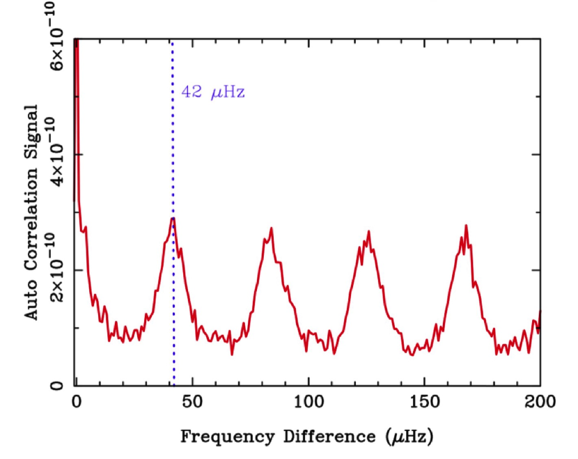
Figure 8: Autocorrelation of power spectrum, showing a 42-$\mu$Hz peak interpreted as half of the large frequency separation between modes.

For solar-like oscillators, the frequency of maximum oscillation power, $\nu_{\rm max}$, has been found to scale as $gT_{\rm eff}^{-1/2}$ (Brown et al., 1991; Kjeldsen & Bedding, 1995; Belkacem et al., 2011), where $g$ is the surface gravity and $T_{\rm eff}$ is the effective temperature of the star. The most obvious spacings in the spectrum are the large frequency separations, $\Delta\nu$. These large separations scale to very good approximation as $\left<\rho\right>^{1/2}$, $\left<\rho\right>\propto M/R^{3}$ being the mean density of the star with mass $M$ and surface radius $R$ (see, e.g., Ulrich, 1986; Christensen-Dalsgaard, 1993).

We used several independent analysis codes to obtain estimates of the average large separation, $\left<\Delta\nu\right>$, and $\nu_{\rm max}$, using automated analysis tools that have been developed, and extensively tested (Christensen-Dalsgaard et al., 2010; Hekker et al., 2010; Huber et al., 2009; Mosser & Appourchaux, 2009; Mathur et al., 2010a; Verner et al., 2011) for application to Kepler data (Chaplin et al., 2011). A final value of each parameter was selected by taking the individual estimate that lay closest to the average over all teams. The uncertainty on the final value was given by adding (in quadrature) the uncertainty on the chosen estimate and the standard deviation over all teams. The final values for $\left<\Delta\nu\right>$ and $\nu_{\rm max}$ were $83.9\pm 0.4\,\rm\mu Hz$ and $1829\pm 54\,\rm\mu Hz$, respectively.

We then provided a first estimate of the properties of the star using a grid-based approach, in which properties were determined by searching among a grid of stellar evolutionary models to get a best fit for the input parameters, which were $\left<\Delta\nu\right>$, $\nu_{\rm max}$, and the spectroscopically estimated $T_{\rm eff}=6650\pm 80\,\rm K$ and [Fe/H]=$-0.07\pm 0.07$ of the star. Descriptions of the grid-based pipelines used in the analysis may be found in Stello et al. (2009); Basu et al. (2010); Gai et al. (2010); Quirion et al. (2011) and Chaplin et al. (2014). The spread in the grid-pipeline results, which reflects differences in, for example, the evolutionary models and input physics, was used to estimate the systematic uncertainties.

The oscillation power envelope of $\theta$ Cyg (Fig. 4) does not have the typical Gaussian-like shape shown by cooler, Sun-like analogues. Instead, it has a plateau, very reminiscent of the extended, flat plateau shown by the oscillation power in the F-type subgiant Procycon A, which has a similar $T_{\rm eff}$ (Arentoft et al., 2008; Bedding et al., 2010b). The shape of the envelope raises potential questions over the robustness of the use of $\nu_{\rm max}$ as a diagnostic for the hottest solar-like oscillators.

Two sets of estimated stellar properties were returned by each grid-pipeline analysis: one in which both $\Delta\nu$ and $\nu_{\rm max}$ were included as seismic inputs; and one in which only $\Delta\nu$ was used.

Both sets returned consistent results for the mass ($M=1.35\pm 0.04\,\rm M_{\odot}$), $\log\,g$ ($4.208\pm 0.006\,\rm dex$) and age (${\rm\tau_{\odot}}=1.7\pm 0.4\,\rm Gyr$), but not the radius. There, using $\Delta\nu$ only yielded a radius of $R=1.51\pm 0.02\,\rm R_{\odot}$, in good agreement with the interferometric value (Section 4), while inclusion of $\nu_{\rm max}$ changed the best-fitting radius to $R=1.58\pm 0.03\,\rm R_{\odot}$, an increase of just under $2\sigma$ (combined uncertainty). This difference – albeit somewhat marginal – could be reconciled by a lower observed $\nu_{\rm max}$.

6 Estimated mode linewidths and amplitudes

We used theoretical calculations to estimate the linear damping rates $\eta(\nu)$ and amplitudes of the radial pulsation modes. The equilibrium and linear stability computations were similar to those by Chaplin et al. (2005, see also ). Convection was treated by means of a nonlocal, time-dependent generalization of Gough’s (1977a,b) mixing-length formulation. The nonlocal formulation includes two more parameters, $a$ and $b$, in addition to the mixing-length parameter, which control respectively the spatial coherence of the ensemble of eddies contributing to the turbulent fluxes of heat and momentum and the degree to which the turbulent fluxes are coupled to the local stratification. The momentum flux (turbulent pressure) was treated consistently in both the equilibrium and linear pulsation calculations. The mixing-length parameter was calibrated to obtain the same surface convection-zone depth as suggested by the AMP evolutionary calculations discussed in the Section 8.2. The nonlocal parameters, $a$ and $b$, were calibrated to reproduce the same maximum value of the turbulent pressure in the superadiabatic boundary layer as suggested by the grid results of three-dimensional (3D) convection simulations reported by Trampedach et al. (2014). Gough’s (1977a,b) time-dependent convection formulation includes also the anisotropy parameter $\Phi\equiv u_{i}u_{i}/w^{2}$, where $u_{i}=(u,v,w)$ is the convective velocity vector, for describing the anisotropy of the turbulent velocity field. In our model computations we varied $\Phi$ with stellar depth (Houdek et al. in preparation), guided by the 3D simulations by Trampedach et al. (2014), and calibrated the value such as to obtain a good agreement between modelled linear damping rates and measured linewidths (see Figure 9). The remaining model computations were as described in Chaplin et al. (2005).

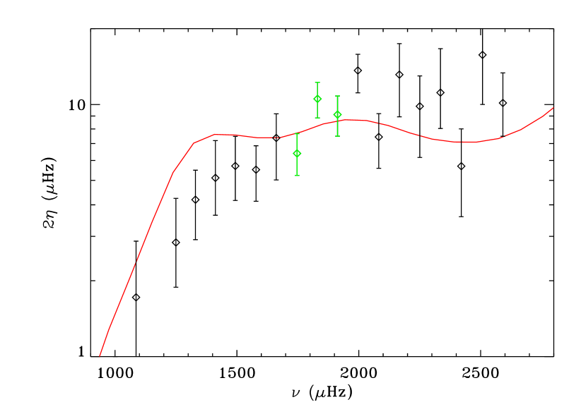
Figure 9: Twice the theoretical linear damping rates for radial modes as a function of frequency calculated for AMP Model 1 (Table 3) with mass $M=1.39$ M_⊙, luminosity $L=4.215$ L_⊙, effective temperature $T_{\rm eff}=6753$ K, and helium and heavy-element abundances by mass $X=0.7055$ and $Z=0.01845$ (solid red line). The diamond symbols show the measured linewidths for observed radial modes of Table 2, with 3$\sigma$ error bars. The green symbols indicate the three most prominent consecutive modes.

Figure 9 shows twice the value of the theoretical linear damping rates (roughly equal to the full width at half maximum of the spectral peaks in the acoustic power spectrum) as a function of frequency for a model with the global parameters of AMP Model 1 of Table 3. The theoretical values are in good agreement with the range of measured mean linewidths, 8.4 $\pm$ 0.3 $\mu$Hz, of the three most prominent modes (see Section 7 below). near $\nu_{\rm max}\simeq 1800\,\mu$Hz.

Amplitudes were estimated according to the scaling relation reported by Kjeldsen & Bedding (1995), but also with the more involved stochastic excitation model of Chaplin et al. (2005, see also ). In this model the acoustic energy-supply rate was estimated from the fluctuating Reynolds stresses adopting a Gaussian frequency factor and a Kolmogorov spectrum for the spatial scales (see e.g., Houdek, 2006, 2010; Samadi et al., 2007). Kjeldsen & Bedding’s scaling relation suggest a maximum luminosity (intensity) amplitude of about $2.2$ times solar, which is in reasonable agreement with the observed value of $4-5\,$ppm, assuming a maximum solar amplitude of $2.5\,$ppm (Chaplin et al., 2011). The adopted stochastic excitation model provides a maximum amplitude of about $2.6$ times solar, which is slightly larger than the value from the scaling relation. The overestimation of pulsation amplitudes in relatively ‘hot’ stars has been reported before, for example, for Procyon A, (see, e.g., Houdek, 2006; Appourchaux et al., 2010). Note that the most recent amplitude-scaling relation anchored on open-cluster red giants (Stello et al., 2011), which agrees with observations of main-sequence stars (Huber et al., 2011), predicts 5.1 ppm for $\theta$ Cyg, in good agreement with its observed value.

7 Mode Identification and Peak Bagging

7.1 Échelle diagram

A convenient way to visualise solar-like oscillations is with the échelle diagram (Grec, Fossat & Pomerantz, 1983), which makes use of the nearly-regular pattern exhibited by the modes. In these diagrams, the power spectrum is split up into slices of width $\Delta\nu$, which are stacked on top of each other. Modes of the same angular degree $l$ form nearly vertical ridges in these diagrams. The échelle diagram for $\theta$ Cyg is shown in Figure 10. The width of the échelle diagram is the large separation, $\Delta\nu=83.9$ $\mu\mathrm{Hz}$. The échelle diagram can be useful for finding weak modes that fall along the ridges, and also for making the mode identification, that is, determining the $l$ value of each mode.

In stars like the Sun, the mode identification can be trivially made from the échelle diagram because the $l=0$ and $l=2$ modes form a closely spaced pair of ridges that is well-separated from the $l=1$ modes. However, in hotter stars we see stronger mode damping, leading to shorter mode lifetimes and larger linewidths (Chaplin et al., 2009; Baudin et al., 2011; Appourchaux et al., 2012a; Corsaro et al., 2013). This blurs the $l=0,2$ pairs into a single ridge that is very similar in appearance to the $l=1$ ridge. This problem was first observed in the CoRoT F star HD 49933 (Appourchaux et al., 2008) and subsequently in other CoRoT stars (Barban et al., 2009; García et al., 2009), Procyon (Bedding et al., 2010b), and many Kepler stars (e.g., Mathur et al., 2012; Appourchaux et al., 2012b; Metcalfe et al., 2014). From Figure 10 it is clear that $\theta$ Cyg also suffers from this problem. Without a clear mode identification, the prospects for asteroseismology on this target are severely impeded.

Several methods have been proposed to resolve this mode identification ambiguity from échelle diagrams. One method is to attempt to fit both possible scenarios. A more likely fit should arise for the correct identification as it will better account for the additional power provided by the $l=2$ modes to one of the ridges. However, this method can run into difficulties with low signal-to-noise observations, or with short observations in which the Lorentzian mode profiles have not been well resolved. Rotational splitting, as well as wide linewidths and short lifetimes, will also create complications for this method.

Despite these difficulties, we attempted to fit the two possible mode identifications (or scenarios) using the Markov Chain Monte Carlo (MCMC) method and a Bayesian framework. A MCMC algorithm performs a random walk in the parameter space and explores the topology of the posteriori distribution (within bounds defined by the priors). This method enabled us to determine the full probability distribution of each of the parameters and to determine the so-called evidence (e.g. Benomar et al., 2009a, b). The evidence for the two mode identifications can be compared in order to evaluate the odds of the competing scenarios (hereafter referred as scenario A and scenario B) in terms of probability. Scenario A corresponds to $l=0$ at $\approx 1038$ $\mu$Hz (or $\varepsilon$ is 1.4), and scenario B corresponds to $l=0$ at $\approx 1086$ $\mu$Hz (or $\varepsilon$ is 0.9). With a probability of 70%, we found that scenario B is only marginally more likely.

7.2 $\varepsilon$ parameter

An alternative method has been introduced by White et al. (2012) following on from work by Bedding et al. (2010b), which uses the absolute mode frequencies, as encoded in the parameter $\varepsilon$. The value of $\varepsilon$ is determined by the phase shifts of the oscillations as they are reflected at their upper and lower turning points. In the échelle diagram, $\varepsilon$ can be visualized as the fractional position of the $l=0$ ridge across the diagram. The left ridge in Figure 10 is approximately 40% across the échelle diagram, so if this ridge is due to $l=0$ modes then the value of $\varepsilon$ is 1.4. We will refer to this as Scenario A. Alternatively, if the right ridge is due to $l=0$ modes (Scenario B), then the value of $\varepsilon$ is 0.9, since this ridge is approximately 90% across the échelle diagram. If it is known which value $\varepsilon$ should take, then the correct mode identification will be known.

It has been found that a relationship exists between $\varepsilon$ and effective temperature, $T_{\mathrm{eff}}$, both in models (White et al., 2011a) and observationally (White et al., 2011b). Furthermore, since a relation also exists between $T_{\mathrm{eff}}$ and mode line width, $\Gamma$ (Chaplin et al., 2009; Baudin et al., 2011; Appourchaux et al., 2012a; Corsaro et al., 2013), there is also a relation between $\varepsilon$ and $\Gamma$ (White et al., 2011b). Given these observed relationships between $\varepsilon$, $T_{\mathrm{eff}}$ and $\Gamma$ measured from an ensemble of stars, and the measured values of $T_{\mathrm{eff}}$ and $\Gamma$ in $\theta$ Cyg, the likelihood of obtaining either possible value of $\varepsilon$ ($\varepsilon_{\mathrm{A}}$ and $\varepsilon_{\mathrm{B}}$) can be calculated.

Following the method of White et al. (2012), we measured the ridge frequency centroids from the peaks of the heavily smoothed power spectrum. We perform a linear least-squares fit to the frequencies, weighted by a Gaussian window centered at $\nu_{\rm max}$ with FWHM of 0.25 $\nu_{\rm max}$, to determine the values of $\Delta\nu$, $\varepsilon_{\mathrm{A}}$ (1.40$\pm$0.04) and $\varepsilon_{\mathrm{B}}$ (0.90$\pm$0.04). The average linewidth, $\Gamma$ of the three highest amplitude modes is 8.4 $\pm$ 0.3 $\mu$Hz. The positions of $\theta$ Cyg in the $\varepsilon$ – $T_{\mathrm{eff}}$ and $\varepsilon$ – $\Gamma$ planes are shown in Fig. 11. We find the most likely scenario to be Scenario B, with a probability of $99.9$% (calculated in a Bayesian framework described in White et al. (2012)). According to Mosser et al. (2013), who compare the asymptotic and global seismic parameters, only scenario B with $\varepsilon\simeq 0.9$ is possible for a main-sequence star as massive as $\theta$ Cyg. Table 2 lists the frequencies for that most likely scenario.

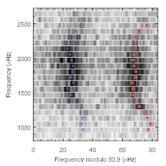
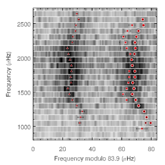
Figure 10: Échelle diagram of $\theta$ Cyg. Left: The blue triangles and red circles show the central frequencies along each ridge in the diagram. Blue triangles correspond to the $l$ = 0 ridge in Scenario A, while red circles correspond to the $l$ = 0 ridge in Scenario B. Right: Échelle diagram of $\theta$ Cyg showing identified frequencies for Scenario B in red. Modes are identified as $l$= 0 (circles), $l$= 1 (triangles), and $l$= 2 (squares). For reference in both figures, a smoothed gray-scale map of the power spectrum is shown in the background.

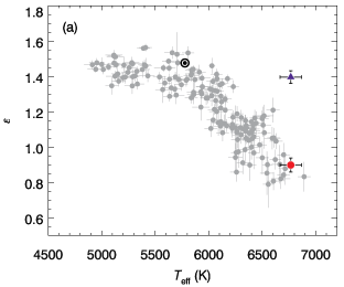
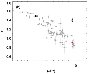
Figure 11: The possible locations of $\theta$ Cyg (blue triangles for Scenario A and red circles for Scenario B) in the (a) $\varepsilon$ – $T_{\mathrm{eff}}$ plane and (b) $\varepsilon$ – $\Gamma$ plane. Grey points are Kepler stars from White et al. (2012). The Sun is marked by its usual symbol. This figure shows that Scenario B is the more likely of the two discussed in Section 7, since an $\varepsilon$ value of $\sim$ 0.9 (as opposed to $\sim$ 1.4) for $\theta$ Cyg places it in line with the other Kepler stars.

7.3 Peak bagging

Individual pulsation frequencies probe the stellar interior, so that by taking them into account, it is possible to improve the precision on the global fundamental parameters of the star. This however requires to measure these frequencies precisely and accurately using the so-called peak-bagging technique. Peak bagging could be performed using several statistical methods. The most common is the Maximum Likelihood Estimator (MLE) approach (Anderson et al., 1990) and has been thoroughly used to analyze the low-degree global acoustic oscillations of the Sun (see, e.g., Chaplin et al., 1996).

Although fast, the MLE is only suited in cases where the likelihood function has a well defined single maximum so that convergence towards an unbiased measure of the fitted parameters is ensured (Appourchaux et al., 1998). Unfortunately, stellar pulsations often have much lower signal-to-noise ratio than solar pulsations, so that the likelihood may have several local maxima. In this situation, the MLE may not converge towards the true absolute maximum of probability.

Conversely, the Bayesian approaches that rely on sampling algorithms such as the MCMC do not suffer from convergence issues (Benomar et al., 2009a, b; Handberg & Campante, 2011). This is because whenever local maxima of probability exist, these are sampled and become evident on the posterior probability density function of the fitted parameters.

In order to get reliable estimates of the mode frequencies for Scenario B, we choose to use such a Bayesian approach. The power spectrum of each star was modelled as a sum of Lorentzian profiles, with frequency, height and width as free parameters. The fit also included the rotational splitting and the stellar inclination as additional free parameters. The noise background function was described by the sum of two Harvey-like profiles (Harvey, 1985) plus a white noise. Table 2 lists the median of the frequencies obtained from the fit the MCMC algorithm, along with the $1\sigma$ uncertainty.

8 Stellar Models Derived from $p$ Modes and Observational Constraints

We explored seismic models for $\theta$ Cyg matching the constraints from spectroscopic and interferometric constraints, as well as the $p$-mode frequencies and mode identifications derived from the Kepler data, using several different methods and stellar evolution and pulsation codes, as described below.

8.1 Results from YREC Stellar Modeling Grid

We use the Yale Rotating Stellar Evolution Code, YREC (Demarque et al., 2008), to calculate a grid of stellar models and their frequencies using a Monte Carlo algorithm to survey the parameter space constrained by the $\theta$ Cyg spectroscopic and interferometric observations summarized in Table 3. This Yale Monte Carlo Method (YMCM) is described in more detail by Silva Aguirre et al. (2015). The Scenario B frequencies of Table 2 are used as seismic constraints. The models are constructed using the OPAL equation of state (Rogers & Nayfonov, 2002), OPAL high-temperature opacities (Iglesias & Rogers, 1996), and Ferguson et al. (2005) low-temperature opacities. Nuclear reaction rates are from Adelberger et al. (1998) except for the ¹⁴N$(p,\gamma)^{15}$O reaction for which the rate of Formicola et al. (2004) is adopted. Convection was treated using the mixing-length formalism of Böhm-Vitense (1958). Models are constructed with a core overshoot of 0.2 pressure scale heights ($H_{p}$) unless the convective core size is less than $0.2~{}H_{p}$, in which case no overshoot is used. Oscillation frequencies are calculated using the code described by Antia & Basu (1994).

Modeling $\theta$ Cyg poses the usual challenges for an F star. The outer convection zone is relatively thin compared to that of the Sun, which means that unless diffusive settling is switched off, or artificially slowed down, the model soon loses most or all of the helium and metals at the photosphere. As a result models were constructed assuming that the gravitational settling of helium and heavy elements is too slow to affect the models.

These YMCM models use the surface-term correction of Ball & Gizon (2014). The surface term is the frequency-dependent deviation of model frequencies from the observed ones and is caused predominantly because of our inability to model the surface of stars properly. The main shortcoming of the models arises because the effect of turbulence is not included. In the solar case the surface term causes model frequencies to be larger than observed frequencies (see, e.g., Christensen-Dalsgaard et al., 1996). The frequencies of the low-frequency modes match observations, while those of high-frequency modes are larger than the observed ones. It is usually assumed that the surface term for models of stars other than the Sun can be simply scaled from the solar case (Kjeldsen et al., 2008; Ball & Gizon, 2014). For future work, 3-D hydrodynamical modeling (Sonoi et al., 2015) could be used to constrain the surface-effect corrections.

The best-fit models are identified by calculating a $\chi^{2}$ value for the seismic and spectroscopic quantities separately, and adding them together. A likelihood is defined using the total $e^{(-\chi^{2})}$ and then used as a weight to find the mean and standard deviation of the model properties. Table  3 summarizes the mean and standard deviations of properties of the models, as well as the properties of the best-fit (highest likelihood) model. Figure 12 shows the échelle diagram for this best-fit model compared to the observed frequencies.

8.2 Results from AMP Stellar Model Grid Optimization Search

The Asteroseismic Modeling Portal (AMP, Metcalfe et al., 2009) searches for models that minimize the average of the $\chi^{2}$ values for both the seismic and spectroscopic constraints. The AMP has been applied extensively to modeling of other Kepler targets (e.g., Mathur et al., 2012; Metcalfe et al., 2012). Although we ran many models exploring various optimization schemes and the effects of diffusive settling, we present results only for models without diffusive settling of helium or heavier elements, as the models including helium settling produce an unrealistic surface helium abundance, and AMP models do not (yet) include diffusion of heavier elements. As noted in Section 8.1 above, the envelope convection zone in F stars is shallow enough that most of the helium and metals would diffuse from the surface when diffusion is included; since we observe a non-zero metallicity at the surface of $\theta$ Cyg, it follows that some mechanisms, such as convective mixing or radiative levitation, are counteracting diffusive settling. However, it is not physically correct to turn off diffusive settling completely, as evidence from helioseismology supports diffusive settling in the Sun (see, e.g., Christensen-Dalsgaard et al., 1993; Guzik et al., 2005).

The AMP search makes use of an option that optimizes the fit to the frequency separation ratios defined by Roxburgh & Vorontsov (2003), as well as to the individual frequencies using the empirical surface correction of Kjeldsen et al. (2008). The fit to the frequencies is also weighted to de-emphasize the highest frequency modes that are most affected by inadequacies in modeling the stellar surface. For complete details, see Metcalfe et al. (2014). The models use the OPAL (Iglesias & Rogers, 1996) opacities and Grevesse & Noels (1993) abundance mixture, and do not include convective overshooting.

For our first optimization runs, we used Scenario B frequencies of Table 2 and chose constraints on $\theta$ Cyg luminosity $L=4.26$ $\pm$ 0.05 L_⊙ based on bolometric flux estimate and Hipparcos parallax, log $g$ = 4.2 $\pm$ 0.2 (Erspamer & North, 2003), metallicity $-$0.05 $\pm$ 0.15, and radius $R=1.503$ $\pm$ 0.007 R_⊙ (Ligi et al., 2012). Note that these spectroscopic constraints are consistent with, but do not exactly match the final recommended values of Sections 3 and 4. The AMP (and some preliminary YREC) models were being calculated in parallel with the spectroscopic analyses, and the early asteroseismic results were even used to constrain the log $g$ that was used in the spectroscopic analysis. The properties of this best-fit model (Model 1) are summarized in Table 3. Fig. 12 shows the échelle diagram for this model comparing the observed and calculated frequencies.

AMP Model 1 has a temperature at the convection-zone base near 320,000 K, exactly right for $\gamma$ Dor $g$-mode pulsations predicted via the convective-blocking mechanism (see Section 9). Because we did not find any $g$ modes in the $\theta$ Cyg data, we explored additional models with the final spectroscopic and interferometric constraints summarized in Column 2 of Table 3. The properties of a second AMP model are summarized in Table 3. AMP Model 2 gives an excellent fit to the observed frequencies (see Fig. 12). Note that the Model 2 échelle diagram uses the scaled surface corrections of Christensen-Dalsgaard (2012) instead of those of Kjeldsen et al. (2008), improving the match to the high-frequency modes. However, Model 2 has $T_{\rm eff}$ and radius slightly lower than the spectroscopic constraints, resulting in a low mass and luminosity compared to AMP Model 1 or to the YREC models. Model 2 has a rather high initial helium mass fraction (0.291), which combined with a lower metallicity (0.0157) compared to Model 1, results in a temperature at the convection-zone base of $\sim$350,000 K, not much higher than for Model 1, despite the lower mass and $T_{\rm eff}$ of Model 2. Note also that the age of Model 2 is more consistent with that of the best-fit YREC model.

Table 2: $\theta$ Cyg Frequencies ($\mu$Hz) Identified for Scenario B used in Asteroseismic Modeling Portal

$l$ = 0 frequency	$l$ = 1 frequency	$l$ = 2 frequency
1086.36 $\pm$ 0.15	1038.35 $\pm$ 0.82	996.59 $\pm$ 3.82
1167.53 $\pm$ 0.07	1122.87 $\pm$ 1.94	1083.06 $\pm$ 0.25
1249.77 $\pm$ 0.28	1207.90 $\pm$ 1.55
1329.96 $\pm$ 0.20	1288.13 $\pm$ 0.66
1411.84 $\pm$ 0.43	1368.96 $\pm$ 0.31
1493.41 $\pm$ 0.37	1450.85 $\pm$ 0.28	1405.70 $\pm$ 0.87
1578.48 $\pm$ 0.45	1533.79 $\pm$ 0.28	1487.17 $\pm$ 1.49
1661.52 $\pm$ 0.51	1619.81 $\pm$ 0.27	1573.61 $\pm$ 1.39
1746.90 $\pm$ 0.68	1703.47 $\pm$ 0.26	1658.62 $\pm$ 1.33
1830.76 $\pm$ 0.43	1787.82 $\pm$ 0.24	1743.02 $\pm$ 1.18
1912.95 $\pm$ 0.47	1871.74 $\pm$ 0.33	1826.99 $\pm$ 1.05
1996.41 $\pm$ 0.63	1954.68 $\pm$ 0.31
2082.14 $\pm$ 0.59	2037.49 $\pm$ 0.35
2166.77 $\pm$ 0.73	2120.73 $\pm$ 0.31	2079.39 $\pm$ 2.68
2250.35 $\pm$ 0.44	2207.91 $\pm$ 0.40	2160.91 $\pm$ 4.22
2335.22 $\pm$ 0.60	2292.26 $\pm$ 0.41	2243.93 $\pm$ 4.1
2420.55 $\pm$ 0.31	2377.88 $\pm$ 0.49	2326.40 $\pm$ 1.51
2507.82 $\pm$ 0.89	2462.11 $\pm$ 0.46	2413.11 $\pm$ 2.20
2591.20 $\pm$ 0.60	2547.92 $\pm$ 0.58	2500.15 $\pm$ 2.35
	2630.50 $\pm$ 0.71

Table 3: Observationally-Derived Parameters (Sections 3 and 4), and Properties of AMP and YREC Models

	Observations	AMPe	AMPe	YREC Ensemble	YREC
		Model 1	Model 2	Average	Best-Fit Model
Mass (M⊙)		1.39	1.26	1.346 $\pm$ 0.038	1.356
Luminosity (L⊙)		4.215	3.350	4.114 $\pm$ 0.156	4.095
$T_{\rm eff}$ (K)	6697 $\pm$ 78	6753	6477	6700 $\pm$ 49	6700
Radius (R⊙)	1.49 $\pm$ 0.03	1.503	1.457	1.507 $\pm$ 0.016	1.504
log $g$	4.23 $\pm$ 0.03	4.227	4.211	4.210 $\pm$ 0.005	4.216
[Fe/H]	$-$0.02 $\pm$ 0.06
[M/H]		0.028	$-$0.005	$-$0.017 $\pm$ 0.042	$-$0.035
Initial $Y^{a}$		0.276	0.291	0.272 $\pm$ 0.017	0.26475
Initial $Z^{b}$		0.01845	0.0157	$-$0.0158	0.015287
$\alpha$c		1.90	1.52	1.77 $\pm$ 0.14	1.69
Age (Gyr)		0.999	1.568	1.625 $\pm$ 0.171	1.516
$T$ CZd base (K)		320,550	354,200		391,916
$\chi^{2}$ seismicf		9.483	8.860		10.67
$\chi^{2}$ spectroscopicf		0.270	2.414		0.0644

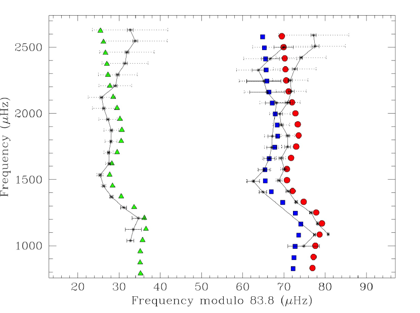
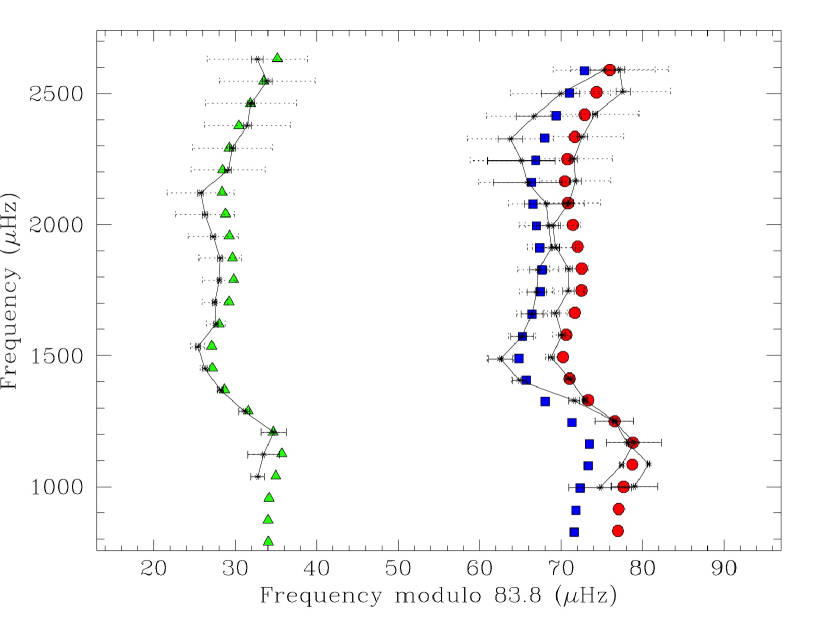
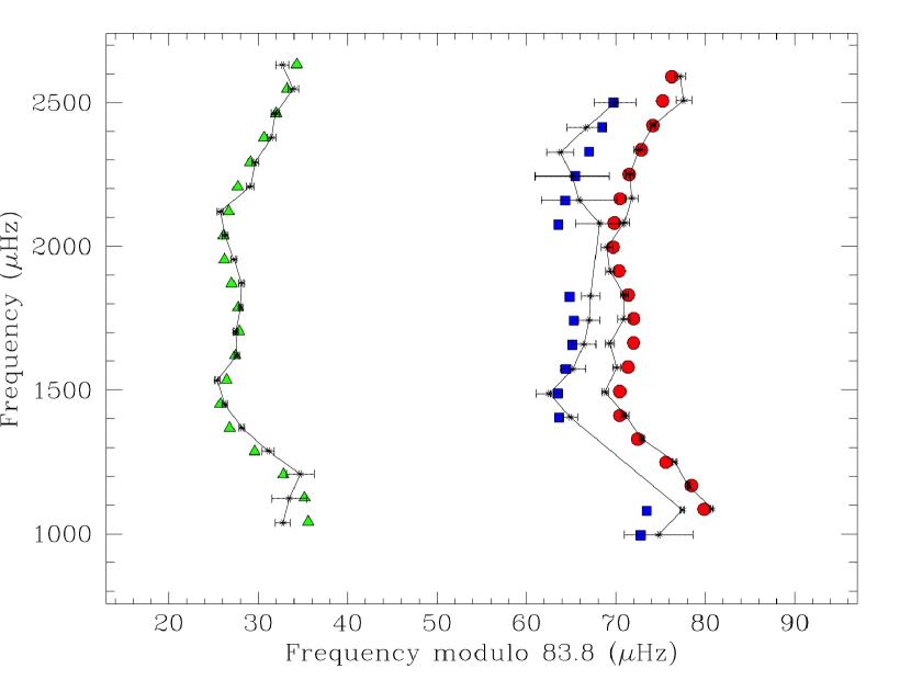
Figure 12: Échelle diagrams comparing the observed oscillation frequencies (connected points) with calculated frequencies of AMP Model 1 and Model 2 (top, left and right, respectively) and best-fit YREC model (bottom). The frequencies are derived from Kepler Q6 and Q8 data (Table 2). Solid error bars indicate the observational uncertainties for each frequency. Colored symbols show the radial ($\circ$), dipole ($\bigtriangleup$), and quadrupole ($\Box$) modes after applying an empirical surface correction. For the AMP models, dotted error bars show the effective uncertainties adopted for the modeling, which treats the surface correction as a systematic error in the model. AMP Model 1 uses the empirical surface corrections of Kjeldsen et al. (2008), while AMP Model 2 uses the scaled solar surface corrections of Christensen-Dalsgaard (2012). The YREC model uses the surface corrections of Ball & Gizon (2014).

9 $\gamma$ Doradus Stars and $g$-mode Predictions

To determine the predicted $\gamma$ Dor-like $g$ mode periods for the models of Table 3, we calculated corresponding models using the updated Iben evolution code (see Guzik et al., 2000). Recalculating the models using the Iben code was expedient, since at present we do not have an interface mapping the structure of the AMP model to the Pesnell (1990) nonadiabatic pulsation code that we use for $g$-mode predictions. We adjusted the mixing length in the Iben-code formulation to match the the radius at approximately the same age as the AMP or YREC best-fit models. The Iben models then also approximately matched the luminosity and envelope convection-zone depth of the AMP or YREC models. The models use OPAL (Iglesias & Rogers, 1996) opacities, Ferguson et al. (2005) low-temperature opacities, and the Grevesse & Noels (1993) abundance mixture. Table  4 gives the properties of the Iben models. While the Iben model initial masses, compositions, and opacities are the same as in the AMP or YREC models, differences in implementation of mixing-length theory, equation of state, opacity table interpolation, nuclear reaction rates, and fundamental physical constants could be responsible for the small differences in model structure.

Table 4: Properties of Iben-Code Models and $g$-Mode Predictions

	Iben	Iben	Iben
	Model 1	Model 2	Model 3
Mass (M⊙)	1.39	1.26	1.356
Luminosity (L⊙)	4.239	3.378	4.119
$T_{\rm eff}$ (K)	6763	6489	6712
Radius (R⊙)	1.503	1.457	1.504
log $g$	4.227	4.211	4.216
Initial $Y^{a}$	0.276	0.291	0.2648
Initial $Z^{b}$	0.01845	0.0157	0.0153
$\alpha$c	1.60	1.30	1.64
Age (Gyr)	1.04	1.60	1.49
$T$ CZd base (K)	319,850	355,500	393,250
Convective Timescalee at CZ base (days)	1.08	1.54	1.88
Largest $g$-mode growth rate per period	3.7e-06	1.4e-06	5.7e-07
$l$ = 1 $g$-mode period range (days)	0.55 to 1.0	0.58 to 1.1	0.59 to 1.0
$l$ = 1 $g$-mode frequency range ($\mu$Hz)	12 to 21	11 to 20	12 to 20
$l$ = 2 $g$-mode period range (days)	0.35 to 0.89	0.34 to 0.65	0.34 to 0.76
$l$ = 2 $g$-mode frequency range ($\mu$Hz)	13 to 33	18 to 34	15 to 34

For $\gamma$ Dor stars, the convective-envelope base temperature that optimizes the growth rates and number of unstable $g$ modes is predicted to be about 300,000 K (see Guzik et al., 2000; Warner et al., 2003). For models with convective envelopes that are too deep, the radiative damping below the convective envelope quenches the pulsation driving; for models with convective envelopes that are too shallow, the convective timescale becomes shorter than the $g$-mode pulsation periods, and convection can adapt during the pulsation cycle to transport radiation, making the convective blocking mechanism ineffective for driving the pulsations.

We calculated the $g$-mode pulsations of the Iben code models using the Pesnell (1990) non-adiabatic pulsation code, which also was used by Guzik et al. (2000) and Warner et al. (2003) to investigate the pulsation driving mechanism for $\gamma$ Dor pulsations and first define the instability-strip location. The Pesnell (1990) code adopts the frozen-convection approximation, which is valid for calculating $g$-mode growth rates, with the driving region at the envelope convection-zone base, only if the convective timescale (defined as the local pressure scale-height divided by the local convective velocity) at the convection-zone base is longer than the pulsation period. This criterion is met for the best-fit models presented here. Table 4 gives the convective timescale at the convective envelope base for each model, and the $g$-mode periods (or alternately, frequencies in $\mu$Hz) for the unstable modes of angular degree $l$=1 and $l$=2. Table 4 also gives the maximum growth rate (fractional change in kinetic energy of the mode) per period for each model, which decreases with increasing convection-zone depth because of increased radiative damping in deeper layers.

If $g$ modes were to be detected in $\theta$ Cyg, this star would become the first hybrid $\gamma$ Dor–solar-like oscillator. However, as discussed in Section 10, $g$ modes have not been detected in the data examined so far. It is possible that $\gamma$ Dor modes may be visible in high-resolution spectroscopic observations, but not in photometry. Brunsden et al. (2015) find for $V=5.74$ $\delta$ Sct/$\gamma$ Dor hybrid star HD 49434 that some $g$ modes found via high-resolution spectroscopy were not detected in CoRoT photometry, and vice versa. Another possibility discussed by Guzik et al. (2000) is that shear dissipation from turbulent viscosity near the convection-zone base or in an overshooting region below the convection zone may be comparable to the driving, and may quench the pulsations. The predicted $g$-mode growth rates of $\sim$10^-6 per period are smaller than typical $\delta$ Sct $p$-mode growth rates of $\sim$10^-3 per period. The models presented here do not take into account diffusive settling, radiative levitation, or changes in abundance mixture that could affect the convection zone depth and $g$-mode driving. $\theta$ Cyg may therefore be important for furthering our understanding of the role of stellar abundances, diffusive settling, and turbulent convection on stellar structure and asteroseismology.

10 Search for $g$ modes in $\theta$ Cyg Data

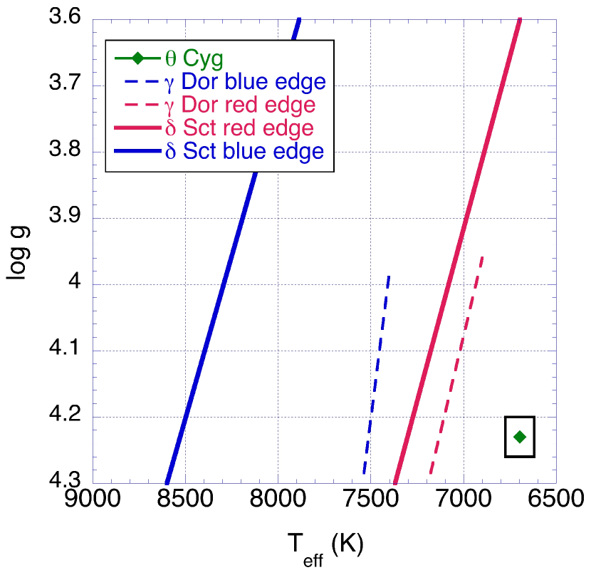
Figure 13: HR diagram location of $\theta$ Cyg relative to $\gamma$ Dor and $\delta$ Sct instability strip edges established from ground-based observations. In this figure $\theta$ Cyg is located at 6697 $\pm$ 78 K, and log $g$ = 4.23 $\pm$ 0.03 (see Section 3).

Figure 13 shows the location of $\theta$ Cyg relative to the instability strip locations established from ground-based discoveries of $\gamma$ Dor and $\delta$ Sct stars (see Uytterhoeven et al., 2011, and references therein). The temperature used for $\theta$ Cyg’s location in this figure is 6697 $\pm$ 78 K based on the spectroscopic observations summarized in Section 3. $\theta$ Cyg’s log $g$ and effective temperature in this figure places it to the right of the red edge of the $\gamma$ Dor instability strip established from pre-Kepler ground-based observations. Taking into account more generous uncertainties on effective temperature and surface gravity, $\theta$ Cyg could be just at the edge of the instability strip. $\gamma$ Dor candidates have been discovered in the Kepler data that appear to lie beyond this $\gamma$ Dor red edge based on Kepler Input Catalog parameters (see, e.g. Uytterhoeven et al., 2011; Guzik et al., 2015). However, the purer sample of Kepler $\gamma$ Dor stars with log $g$ and $T_{\rm eff}$ established from high-resolution spectroscopy (Van Reeth et al., 2015) does fall within the $\gamma$ Dor instability strip established from theory (Bouabid et al., 2013). See, in addition, Niemczura et al. (2015) and Tkachenko et al. (2013), who also do not show $\gamma$ Dor stars beyond this red edge. The theoretically derived instability regions of Bouabid et al. (2013) and Dupret et al. (2005) including time-dependent convection show the red edge extending at log $g$ = 4.2 to $\sim$6760 K, placing $\theta$ Cyg just at the red edge.

In contrast to stochastically excited solar-like oscillations, $g$-mode pulsations excited by the convective blocking mechanism are known to be coherent, resulting in sharp peaks in the Fourier spectrum, with line widths defined by the duration of the observations. Attributing low-frequency signals to $g$ modes requires caution, as other phenomena such as granulation, spots and instrumental effects occur at similar time scales. However it is possible to distinguish between these signatures. The granulation background noise, for example, as observed in many solar-type stars and red giants (e.g., Mathur et al., 2011b) but also in $\delta$ Scuti stars (e.g., Kallinger & Matthews, 2010; Mathur et al., 2011b), has a distinct signature which can be described as the sum of power laws with decreasing amplitude as a function of increasing frequency (e.g., Kallinger & Matthews, 2010). Long-lived stellar spots, on the other hand, which follow the rotation often result in a single peak; however, if latitudinal differential rotation occurs, and/or the spot sizes and lifetimes change, as observed in the Sun, spots can produce a peak with a multiplet structure (Mosser et al., 2009; Mathur et al., 2010b; Ballot et al., 2011; García et al., 2014b) which can be misinterpreted as $g$ modes. In the case of stellar activity, the temporal variability allows to draw a conclusion. Instrumental effects are not easy to identify; however, in the present case, we can compare the light curve of $\theta$ Cyg with that of other stars, observed during the same quarters and we can also exclude very long periods. Also, contamination by background stars needs to be taken into account, especially in the present case, as the collected light is spread over 1600 pixels on the detector.

Visual inspection of the processed light curve (Section 2, Fig. 3) indicates that we might observe rotational modulation due to spots, as discussed by Balona et al. (2011). In the Fourier spectrum, we find a peak at 0.159 d^-1 (1.840 $\mu$Hz), which translates into a period of 6.29 days. If this were a rotational period, using a radius $R=1.5$ R_⊙ and $v\sin{i}$ = $3.4\pm 0.4$ km s^-1 (Section 3), the rotational velocity would be 12 km s^-1 and the inclination angle would be 16 $\pm$ 2 degrees. The frequency at 0.159 c d^-1 is present in both quarters; however at the end of Q8 the amplitude at this frequency starts to diminish, a temporal variability consistent with a changing activity cycle. Rotational frequencies may also be distinguished from $g$-mode frequencies if the modes behave linearly (see, e.g., Thoul et al., 2013), as the rotational frequency would occur with multiple harmonics, whereas the $g$-mode frequency would not.

To search for $g$ modes, we analyzed the short-cadence Q6 and Q8 data separately, and then in combination. Figure 14 shows the amplitude spectrum, and Figure 15 shows a zoom-in of this spectrum for frequencies from 5 to 25 $\mu$Hz (0.43 to 2.16 d^-1). We find one significant peak at 20.56 $\mu$Hz (1.7763 d^-1), which is a good candidate for a $g$ mode, but one peak alone is usually not enough to claim the detection of such pulsation modes. From Kepler observations we know that $\gamma$ Dor stars as well as $\gamma$ Dor/$\delta$ Sct hybrids usually show more than one $g$ mode excited (Tkachenko et al., 2013). In the present case however we can definitely exclude this frequency from being a $g$ mode, because the binned phase plot clearly shows the signature of a binary system, which is around 10 magnitudes fainter than $\theta$ Cyg. Figure 16 shows the binned phase plot folded by 1.7763 d^-1 for the different quarters. Figures 14 and 15 show with vertical dashed gray lines the harmonics of this frequency.

We have not established whether the binary signal is related to the $\theta$ Cyg system. Identifying the source of the binary signal and its relationship to $\theta$ Cyg would require considerable work given the faintness of the source. One could investigate whether the signal is more prominent in the point-spread function by comparing the Fourier transform of data sets with different extraction masks, covering different parts of the point-spread function; if the signal is associated with $\theta$ Cyg, additional radial velocity measurements may also be required.

A question of interest is the effect of the binary signal on the light curve on the derived $p$-mode oscillation properties. In order to affect the signal in the 1000-3000 $\mu$Hz region of the $p$-mode spectrum, the signal would need to be approximately the 50th harmonic of the 1.7763 d^-1 binary frequency. Such high harmonics would not be visible, especially considering that the base frequency is barely significant, as shown in Fig. 15. The $p$-mode amplitudes, converting from ppm²/$\mu$Hz to ppm, are approximately 30 to 100 ppm, while the binary signal harmonics near 250 $\mu$Hz already have amplitudes as low as $\sim$2 ppm, and will become even smaller at higher frequencies.

In addition, simulations have been performed (see supplementary on-line information for Antoci et al., 2011) in the context of KIC 7548479 for artificial data containing coherent non-stochastic signals (binary and $g$ modes) and non-coherent solar-like oscillations, to understand whether prewhitening the coherent signals influences the non-coherent ones. It was found that prewhitening the coherent signals does not affect the solar-like oscillations.

It is interesting that the eclipsing binary orbital frequency is close to one-fourth of the large separation (4 x 20.56 $\mu$Hz = 82.24 $\mu$Hz $\simeq$ 83.9 $\mu$Hz). A single star orbiting $\theta$ Cyg at this period would have an orbital semi-major axis of $\sim$3.2 R_⊙, a little over twice $\theta$ Cyg’s radius. Another possibility is that a binary system with this orbital period is associated with $\theta$ Cyg (see discussion of $\theta$ Cyg B in the Appendix). In either case, it could be considered whether tidal effects could have some effect on the $p$-mode spacing. Tidal effects have been shown to drive modes separated by the orbital frequency in the so-called heartbeat stars (Thompson et al., 2012; Hambleton et al., 2015), but the modes driven are generally in the $g$-mode range. Additional shorter periods are also found in some heartbeat stars, and at least one heartbeat star, KIC 4544587, has some $\delta$ Sct $p$-modes separated by multiples of the orbital frequency (Hambleton et al., 2013) . However, if there were tidal forcing involved, we would expect the pulsation periods to be exact multiple integers of the orbital period, which is not the case for $\theta$ Cyg. Furthermore, such modes would be expected to be coherent, unlike the stochastically excited $p$ modes observed for $\theta$ Cyg. Therefore, we consider an association between the binary frequency and the $\theta$ Cyg $p$ modes to be unlikely.

The binary signal has very small amplitude, barely above the signal-to-noise criterion of 4, which means that if $g$ modes were present they should be visible in the spectrum of Figs. 14 and 15. We have done some tests with the long-cadence data, prewhitening for the binary harmonic, and find no other significant long-period modes.

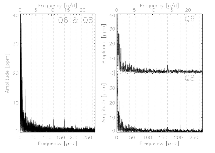
Figure 14: Fourier spectra of the individual quarters and the combined data, with the vertical dashed gray lines indicating the orbital frequency of the background binary and its harmonics. One remaining frequency at $\sim$ 1.7 d^-1 probably is attributable to a background binary (see text and Fig. 16).

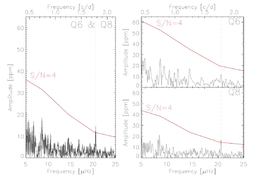
Figure 15: Zoom-in of the region from 5 to 25 $\mu$Hz (0.5 to 2.5 d^-1 ). The red line indicates the S/N (signal-to-noise) = 4.0 significance criterion calculated using Period04 (Lenz & Breger, 2005).

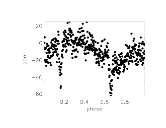
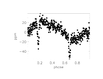
Figure 16: Q6 (left) and Q8 (right) light curve folded at 1.77627 d^-1 ($\sim$20.56 $\mu$Hz), showing that a faint background binary is the likely explanation for this frequency in the power spectrum.

11 Conclusions and Motivation for Continued Study of $\theta$ Cyg

We have analyzed Quarters 6 and 8 of Kepler $\theta$ Cyg data, finding solar-like $p$-modes, and not finding $\gamma$ Dor gravity modes that were initially expected given $\theta$ Cyg’s spectral tye. We have obtained new ground-based spectroscopic and interferometric observations and updated the observational constraints. Stellar models of $\theta$ Cyg that fit the $p$-mode frequencies and spectroscopic and interferometric constraints on $R$, $T_{\mathrm{eff}}$, log $g$, and [M/H] are predicted to show $g$-mode pulsations driven by the convective-blocking mechanism, according to nonadiabatic pulsation models. However, analysis of the light curves did not reveal any $g$ modes.

Reprocessed Kepler observations of $\theta$ Cyg for Quarters 12 through 17 including the pipeline corrections will be available in late 2016. We intend to examine the pixel-by-pixel data to remove the background binary if possible. As noted by Tkachenko et al. (2013) in analysis of their sample of 69 $\gamma$ Dor stars, use of the pixel data eliminated many spurious low frequencies detected using the standard pre-processed light curves. Analyses of a longer time series may reduce noise due to granulation, and more definitively rule out the presence of $g$ modes or identify features in the light curve resulting from rotation and stellar activity. The Kepler observations of $\theta$ Cyg, in conjunction with studies of many other A-F stars observed by Kepler and CoRoT, will be key to understanding the puzzles of $\gamma$ Dor/$\delta$ Sct hybrids and pulsating variables that appear to lie outside of instability regions expected from theoretical models, and to test stellar model physics and possible alternative pulsation driving mechanisms.

Attempting to find $g$ modes in $\theta$ Cyg and other mid-F spectral type stars is worthwhile, as $g$ modes are more sensitive to the stellar interior near the convective core boundary than are $p$ modes. Seismic measurements of convective core size and shape, and the structure of the overshooting region will help reduce uncertainties in stellar ages and understand the roles of penetrative overshooting and diffusive mixing. Progress has already been made in this area for Kepler slowly-pulsating B stars that are $g$ mode pulsators by, e.g., Moravveji et al. (2015), who used the spacings of 19 consecutive $g$ modes in KIC 9526294 to distinguish between models using exponentially decaying vs. a step-function overshooting prescription, and diagnose the need for additional diffusive mixing. However, note that progress is also being made studying convective cores using $p$ modes in low-mass stars (see, e.g. Deheuvels et al., 2016), as the molecular weight gradient outside the convective core introduces a discontinuity in sound-speed profile that is diagnosable with $p$ modes.

The core size and mode frequencies are also affected by rotation that is likely to be more rapid in the core than in the envelope. Van Reeth et al. (2015) discuss $g$-mode periods and spacings for a sample of 67 $\gamma$ Dor stars observed by Kepler, and find correlations between $v~{}\sin i$, $T_{\rm eff}$, period spacing values, and dominant periods. van Reeth et al. (2016, submitted), discuss a method for mode identification of high-order $g$ modes from the period spacing patterns for $\gamma$ Dor stars, allowing to deduce rotation frequency near the core. Bedding et al. (2015) discuss using period échelle diagrams for Kepler $\gamma$ Dor stars to measure period spacings and identify rotationally split multiplets with $l$ = 1 and $l$ = 2. Keen et al. (2015) study KIC 10080943, two hybrid $\delta$ Sct/$\gamma$ Dor stars in a non-eclipsing spectroscopic binary, and are able to use rotational splitting to estimate core rotation rates.

Because $\theta$ Cyg is nearby and bright, and data can be obtained with excellent precision, it is also a worthwhile target for continued long time-series ground- or space-based photometric or spectroscopic observations. With an even longer time series of data (obtainable by a follow-on to the Kepler mission), there is the possibility to study rotational splitting and differential rotation, infer convection zone depth directly from oscillation frequency inversions, measure sin $i$ directly from amplitude differences of rotationally split modes, and investigate possible magnetic activity cycles.

Appendix A The $\theta$ Cygni System

The field around $\theta$ Cyg (Fig. 17) has been examined to identify any stars which might be part of the system. Selected stars are now discussed. For the other stars within 2′ there is insufficient evidence to suggest that they are companions of $\theta$ Cyg.

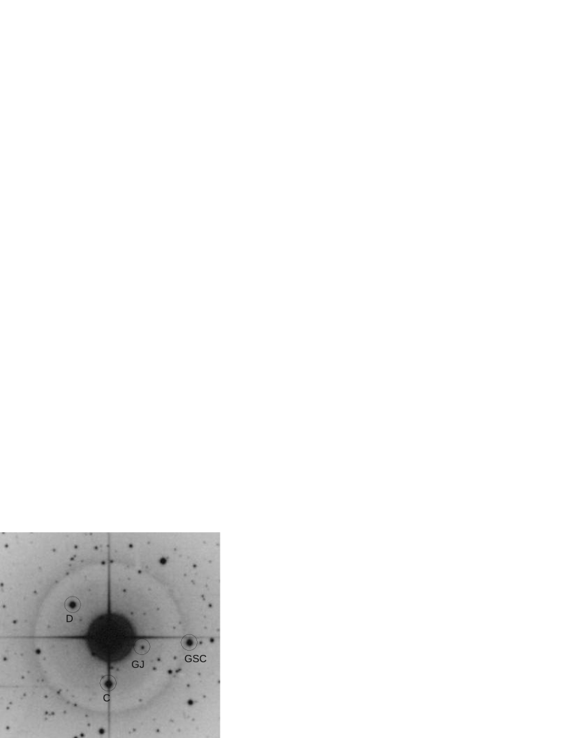
Figure 17: Digitized Sky Survey image showing the field around $\theta$ Cyg AB. The scale of this figure is approximately 5$\frac{1}{4}$ arc minutes wide. The stars discussed in the text are highlighted. GJ is GJ765B and GSC is GSC 03564-00642.

A.1 $\theta$ Cyg A

There is a vast literature on $\theta$ Cyg A, that is summarized in Table 5. This review of the literature prior to the Kepler observations shows that $\theta$ Cyg A is a normal slowly-rotating solar-composition F3V-type star (Gray et al., 2003) with $T_{\mathrm{eff}}$ around 6700$\pm$100 K and $\log g$ around 4.3$\pm$0.1 dex.

Table 5: A summary of parameter determinations of $\theta$ Cyg in the literature. While not all referenced values are new and independent determinations, the compilation does give an indication of the range of values previously found. At the bottom of table the averages and standard deviations are given, in order to indicate the typical scatter in results.

$T_{\mathrm{eff}}$	$\log g$	$[Fe/H]$	Reference
6700			Böhm-Vitense (1978)
7000	4.27	0.07	Philip & Egret (1980)
6545	4.40	-0.21	Thevenin et al. (1986)
6632	4.40	0.10	Boesgaard & Lavery (1986)
6840			Malagnini & Morossi (1990)
6770	4.41		Adelman et al. (1991)
6713			Blackwell & Lynas-Gray (1994)
6725	4.35	0.01	Marsakov & Shevelev (1995)
6462		0.04	Merchant (1966)
6550	4.4	0.00	Thevenin (1998)
6672			Blackwell & Lynas-Gray (1998)
6666			di Benedetto (1998)
6760	4.24		Allende Prieto & Lambert (1999)
6700	4.30	0.01	Cunha et al. (2000)
6640		-0.02	Taylor (2003)
6745	4.21	-0.03	Erspamer & North (2003)
6704	4.35	-0.02	Le Borgne et al. (2003)
6747	4.21	-0.04	Gray et al. (2003)
6594	4.04	-0.03	Valenti & Fischer (2005)
6810		0.1	Ryabchikova (2005)
	4.20		Takeda et al. (2007)
6650		-0.04	Holmberg et al. (2009)
6696	4.29	0.00
$\pm$ 115	$\pm$0.11	$\pm$ 0.08

A.2 $\theta$ Cyg B

The close companion $\theta$ Cyg B (KIC 11918644; 2MASS 19362771+5013419) is listed in the Washington Visual Double Star Catalog (WDS) (Mason et al., 2001) as a magnitude 12.9 star at 3.6″ and PA 44° in 1889. The orbital motion was discussed by Desort et al. (2009), who give a projected separation 46.5 AU, a minimum period of roughly 230 years and a mass from evolutionary codes of 0.35 $M_{\sun}$.

Using the $H$ and $K$ contrasts given in Desort et al. (2009), we estimate that $H\sim 8.3$ and $K\sim 8.0$. Using $V\sim 12.9$, an approximate bolometric flux of $F_{\rm bol}\sim 1.0^{-12}$ W m^-2 was obtained. Using the IRFM (Blackwell & Shallis, 1977), we estimate that $T_{\mathrm{eff}}$ = $3000\sim 3500$ K and an angular diameter of $\sim 0.18$ mas. Using Hipparcos distance, we get $\log L/L_{\sun}\sim-2.0$, $M_{\rm bol}\sim 9.7$ and $R\sim 0.36\,R_{\sun}$.

The approximate position of $\theta$ Cyg B in the HR diagram is shown in Fig. 18.

In Section 10 we identified a potential short-period binary within the Kepler mask. If this star is the binary and has equal components, then the individual stars have mass of $\sim 0.18\,M_{\sun}$ and radii of $\sim 0.25\,R_{\sun}$. The individual luminosities will be 0.3 dex lower, placing them closer to the isochrone in Fig. 18.

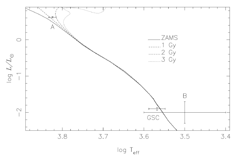
Figure 18: Hertzsprung-Russell diagram for $\theta$ Cyg system, showing components A and B, plus the common proper-motion companion GSC 03564-00642. Models are from Marigo et al. (2008).

A.3 $\theta$ Cyg C

The Bright Star Catalogue states that WDS 19364+5013AC (KIC 11918629) is a mag. 11.6 optical companion at 29.9″ and PA 186° in 1852. The current separation of $\sim$1′ supports this conclusion.

A.4 $\theta$ Cyg D

WDS 19364+5013AD (KIC 11918668) is a mag. 12.5 $T_{\mathrm{eff}}$ = 6800 K star at 82.1″ and PA 40° in 1923. With a current separation of 1.17′ and PA 50° this is an optical companion.

A.5 GJ 765B

With similar proper motions (Lépine & Shara (2005)), the star GJ 765B (2MASS 19362286+5013034; KIC 11918614) could be a common proper motion companion. Optical photometry ($V\sim 13.03$) and 2MASS suggest that this could be a hot star (A or B-type). The estimated $\log L/L_{\sun}\sim-2.0$ and $M_{\rm bol}\sim 9.9$ are inconsistent for a main-sequence star, but not a subdwarf.

Alternatively, this star might actually be 2MASS19362147+5012599 (KIC 11918601), but for the same $V$ magnitude this would also be a hot star with low luminosity ($\log L/L_{\sun}\sim-2.4$ and $M_{\rm bol}\sim 10.7$).

Further observations are required to confirm the nature of these stars, in order to determine whether or not this is a common proper motion companion.

A.6 GSC 03564-00642

Young & Farnsworth (1924) suggested that a faint companion (GSC 03564-00642, 2MASS J19361440+5013096; KIC 11918550) 2′ west of $\theta$ Cyg A was physical. Bidelman (1980) confirmed that the spectral type, M2/3 is consistent with this suggestion. The proper motion is slightly different from $\theta$ Cyg A, but not totally inconsistent with this suggestion considering the range of values in the various catalogues.

Available broad-band photometry, suggests $T_{\mathrm{eff}}\sim 3700$ K, $F_{\mathrm{bol}}\sim 1.2^{-12}$ W m^-2 and angular diameter $0.14\pm 0.03$ mas. Using the Hipparcos distance to $\theta$ Cyg A, we get $\log L/L_{\sun}=-1.90\pm 0.04$, $M_{\rm bol}=9.50\pm 0.11$ and $R=0.28\pm 0.06$ R_☉. The position in HR Diagram is also shown in Fig. 18, and the star appears to be part of the $\theta$ Cygni system.

References

- Aerts, Christensen-Dalsgaard & Kurtz (2010) Aerts, C., Christensen-Dalsgaard, J., Kurtz, D. W. 2010, Asteroseismology, Springer Science Publisher, Dordrecht
- Adelberger et al. (1998) Adelberger E. G., et al. 1998, Rev. Mod. Phys., 70, 1265
- Adelman et al. (1991) Adelman, S. J., Bolcal, C., Kocer, D., & Hill, G. 1991, MNRAS, 252, 329
- Alekseeva et al. (1997) Alekseeva, G. A., Arkharov, A. A., Galkin, V. D., et al. 1997, VizieR Online Data Catalog, 3201
- Alexander & Ferguson (1994) Alexander, D. R., & Ferguson, J. W. 1994, ApJ, 437, 879
- Allende Prieto & Lambert (1999) Allende Prieto, C., & Lambert, D. L. 1999, A&A, 352, 555
- Anderson et al. (1990) Anderson, E. R., Duvall, T. L., Jr., & Jefferies, S. M. 1990, ApJ, 364, 699
- Antia & Basu (1994) Antia, H. M., & Basu, S. 1994, A&AS, 107, 421
- Antoci et al. (2011) Antoci, V., Handler, G., Campante, T. L., et al. 2011, Nature, 477, 570
- Appourchaux et al. (1998) Appourchaux, T., Gizon, L., & Rabello-Soares, M.-C. 1998, A&AS, 132, 107
- Appourchaux et al. (2012b) Appourchaux, T., Chaplin, W. J., García, R. A., et al. 2012b, A&A, 543, A54
- Appourchaux et al. (2008) Appourchaux, T., Michel, E., Auvergne, M., et al. 2008, A&A, 488, 705
- Appourchaux et al. (2010) Appourchaux, T., Belkacem, K., Broomhall, A.-M., et al. 2010, A&A Rev., 18, 197
- Appourchaux et al. (2012a) Appourchaux, T., et al. 2012a, A&A, 537, A134
- Arentoft et al. (2008) Arentoft, T., Kjeldsen, H., Bedding, T. R., et al., 2008, ApJ687, 1180
- Asplund et al. (2009) Asplund, M., Grevesse, N., Sauval, A. J., & Scott, P. 2009, ARA&A, 47, 481 (AGSS09)
- Asplund et al. (2005) Asplund, M. et al. 2005, ASPC 336, 25 (AGS05)
- Baker & Kippenhahn (1965) Baker, N., & Kippenhahn, R. 1965, ApJ, 142, 868
- Ball & Gizon (2014) Ball, W. H., & Gizon, L. 2014, A&A, 568, A123
- Ballot et al. (2011) Ballot, J., Gizon, L., Samadi, R., et al. 2011, A&A, 530, A97
- Balmforth (1992) Balmforth N.J. 1992, MNRAS, 255, 603
- Balona et al. (2011) Balona, L. A., Guzik, J. A., Uytterhoeven, K., et al. 2011, MNRAS, 415, 3531
- Böhm-Vitense (1958) Böhm-Vitense, E. 1958, Zeitschrift für Astrophysik, 46, 108
- Böhm-Vitense (1978) Böhm-Vitense, E. 1978, ApJ, 223, 509
- Barban et al. (2009) Barban, C., et al. 2009, A&A, 506, 51
- Basu & Antia (2008) Basu, S. & Antia, H.M. 2008, Phys. Rep., 457, 217
- Basu et al. (2010) Basu, S., Chaplin, W. J., Elsworth, Y., 2010, ApJ, 710, 1596
- Baudin et al. (2011) Baudin, F., et al. 2011, A&A, 529, A84
- Bedding et al. (2010b) Bedding, T. R., Kjeldsen, H., Campante, T. L., et al., 2010b, ApJ, 713, 935
- Bedding & Kjeldsen (2010a) Bedding, T. R., & Kjeldsen, H. 2010a, Communications in Asteroseismology, 161, 3
- Bedding et al. (2015) Bedding, T. R., Murphy, S. J., Colman, I. L., & Kurtz, D. W. 2015, European Physical Journal Web of Conferences, 101, 01005
- Belkacem et al. (2011) Belkacem, K., Goupil, M. J., Dupret, M. A., et al. 2011, A&A, 530, A142
- Belkacem (2012) Belkacem, K. 2012, SF2A-2012: Proceedings of the Annual meeting of the French Society of Astronomy and Astrophysics, 173
- Benomar et al. (2009a) Benomar, O., Appourchaux, T., & Baudin, F. 2009, A&A, 506, 15
- Benomar et al. (2009b) Benomar, O., Baudin, F., Campante, T. L., et al. 2009, A&A, 507, L13
- Bernacca & Perinotto (1970) Bernacca, P. L., & Perinotto, M. 1970, Contributions dell’Osservatorio Astrofisica dell’Universita di Padova in Asiago, 239, 1
- Bidelman (1980) Bidelman, W. P. 1980, PASP, 92, 345
- Blackwell & Lynas-Gray (1994) Blackwell, D. E., & Lynas-Gray, A. E. 1994, A&A, 282, 899
- Blackwell & Lynas-Gray (1998) Blackwell, D. E., & Lynas-Gray, A. E. 1998, A&AS, 129, 505
- Blackwell & Shallis (1977) Blackwell, D.E. &Shallis, M.J., 1977, MNRAS, 180, 177
- Blackwell et al. (1990) Blackwell, D. E., Petford, A. D., Arribas, S., Haddock, D. J., & Selby, M. J. 1990, A&A, 232, 396
- Boesgaard & Lavery (1986) Boesgaard, A. M., & Lavery, R. J. 1986, ApJ, 309, 762
- Bond et al. (2015) Bond, H. E., Gilliland, R. L., Schaefer, G. H., et al. 2015, ApJ, 813, 106
- Borucki et al. (2010) Borucki, W.J., et al. 2010, Science, 327, 977
- Bouabid et al. (2013) Bouabid, M.-P., Dupret, M.-A., Salmon, S., et al. 2013, MNRAS, 429, 2500
- Boyajian et al. (2012) Boyajian, T. S., McAlister, H. A., van Belle, G., et al. 2012, ApJ, 746, 101
- Breger (1976) Breger, M. 1976, ApJS, 32, 7
- Brown et al. (1991) Brown, T. M., Gilliland, R. L., Noyes, R. W., Ramsey, L. W., 1991, ApJ, 368, 599
- Brown et al. (2011) Brown, T. M., Latham, D. W., Everett, M. E., & Esquerdo, G. A. 2011, AJ, 142, 112
- Brunsden et al. (2015) Brunsden, E., Pollard, K. R., Cottrell, P. L., et al. 2015, MNRAS, 447, 2970
- Bruntt et al. (2010a) Bruntt, H., Bedding, T. R., Quirion, P.-O., et al. 2010a, MNRAS, 405, 1907
- Bruntt et al. (2010b) Bruntt, H., Deleuil, M., Fridlund, M., et al. 2010b, A&A, 519, A51
- Buchhave et al. (2012) Buchhave, L. A., Latham, D. W., Johansen, A., et al. 2012, Nature, 486, 375
- Campante et al. (2011) Campante, T. L., Handberg, R., Mathur, S., et al. 2011, A&A, 534, A6
- Casagrande et al. (2010) Casagrande, L., Ramírez, I., Meléndez, J., Bessell, M., & Asplund, M. 2010, A&A, 512, A54
- Castelli et al. (1997) Castelli, F., Gratton, R. G. & Kurucz, R. L., 1997, A&A, 318, 841
- Chaplin et al. (1996) Chaplin, W. J., Elsworth, Y., Howe, R., et al. 1996, MNRAS, 280, 849
- Chaplin et al. (2005) Chaplin W., Houdek, G., Elsworth, Y., Gough, D.O., Isaac, G.R., New, R., 2005, MNRAS, 360, 859
- Chaplin et al. (2009) Chaplin, W. J., Houdek, G., Karoff, C., Elsworth, Y., & New, R. 2009, A&A, 500, L21
- Chaplin et al. (2011) Chaplin, W. J., Kjeldsen, H., Christensen-Dalsgaard, J., 2011, Science, 332, 213
- Chaplin et al. (2011) Chaplin, W. J., Kjeldsen, H., Bedding, T. R., et al. 2011, ApJ, 732, 54
- Chaplin et al. (2014) Chaplin, W. J., Basu, S., Huber, D., et al. 2014, ApJS, 210, 1
- Christensen-Dalsgaard (1982) Christensen-Dalsgaard, J. 1982, MNRAS, 199, 735
- Christensen-Dalsgaard et al. (1991) Christensen-Dalsgaard, J., Gough, D. O., & Thompson, M. J. 1991, ApJ, 378, 413
- Christensen-Dalsgaard et al. (1996) Christensen-Dalsgaard, J. et al. 1996, Science, 272, 1286
- Christensen-Dalsgaard (1993) Christensen-Dalsgaard, J. 1993, ASP Conf. 42, 347
- Christensen-Dalsgaard et al. (1993) Christensen-Dalsgaard, J., Proffitt, C. R., & Thompson, M. J. 1993, ApJ, 403, L75
- Christensen-Dalsgaard et al. (2010) Christensen-Dalsgaard, J., Kjeldsen, H., Brown, T. M., et al., 2010, ApJ, 713, L164
- Christensen-Dalsgaard (2012) Christensen-Dalsgaard, J. 2012, Astronomische Nachrichten, 333, 914
- Corsaro et al. (2013) Corsaro, E., Fröhlich, H.-E., Bonanno, A., et al. 2013, MNRAS, 430, 2313
- Cunha et al. (2000) Cunha, K., Smith, V. V., Boesgaard, A. M., & Lambert, D. L. 2000, ApJ, 530, 939
- Demarque et al. (2008) Demarque, P., Guenther, D. B., Li, L. H., Mazumdar, A., Straka, C. W. 2008, Ap&SS, 316, 311
- Desort et al. (2009) Desort, M., Lagrange, A.-M., Galland, F., et al. 2009, A&A, 506, 1469
- Deheuvels et al. (2016) Deheuvels, S., Brandão, I., Silva Aguirre, V., et al. 2016, arXiv:1603.02332
- Doyle et al. (2013) Doyle, A. P., Smalley, B., Maxted, P. F. L., et al. 2013, MNRAS, 428, 3164
- Doyle et al. (2014) Doyle, A. P., Davies, G. R., Smalley, B., Chaplin, W. J., & Elsworth, Y. 2014, MNRAS, 444, 3592
- di Benedetto (1998) di Benedetto, G. P. 1998, A&A, 339, 858
- Dupret et al. (2005) Dupret, M.-A., Grigahcène, A., Garrido, R., Gabriel, M., & Scuflaire, R. 2005, A&A, 435, 927
- Eggleton et al. (1973) Eggleton, P. P., Faulkner, J., & Flannery, B. P. 1973, A&A, 23, 325
- Erspamer & North (2003) Erspamer, D., & North, P. 2003, A&A, 398, 1121
- Ferguson et al. (2005) Ferguson, J. W., Alexander, D. R., Allard, F., et al. 2005, ApJ, 623, 585
- Formicola et al. (2004) Formicola A., et al. 2004, Physics Letters B, 591, 61
- Frasca et al. (2006) Frasca, A., Guillout, P., Marilli, E., et al. 2006, A&A, 454, 301
- Głȩbocki & Gnaciński (2005) Głȩbocki, R., & Gnaciński, P. 2005, 13th Cambridge Workshop on Cool Stars, Stellar Systems and the Sun, 560, 571
- Gai et al. (2010) Gai, N., Basu, S., Chaplin, W. J., Elsworth, Y., 2011, ApJ, 730, 63
- García et al. (2009) García, R. A., et al. 2009, A&A, 506, 41
- García et al. (2011) García R. A., Hekker, S., Stello, D., et al. 2011, MNRAS, 414, L6
- García et al. (2014a) García, R. A., Mathur, S., Pires, S., et al. 2014, A&A, 568, A10
- García et al. (2014b) García, R. A., Ceillier, T., Salabert, D., et al. 2014, A&A, 572, A34
- Gilliland et al. (2010a) Gilliland, R. et al. 2010a, PASP, 122, 131
- Gilliland et al. (2010a) Gilliland, R. L., Brown, T. M., Christensen-Dalsgaard, J., et al. 2010, PASP, 122, 131
- Gilliland et al. (2010b) Gilliland, R. L., Jenkins, J. M., Borucki, W. J., et al. 2010b, ApJ, 713, L160
- Glushneva et al. (1998) Glushneva, I. N., Doroshenko, V. T., Fetisova, T. S., et al. 1998, VizieR Online Data Catalog, 3208
- Gómez Maqueo Chew et al. (2013) Gómez Maqueo Chew, Y., Faedi, F., Cargile, P., et al. 2013, ApJ, 768, 79
- Gough (1977a) Gough D.O. 1977a, ApJ, 214, 196
- Gough (1977b) Gough D.O. 1977b, In: Problems of Stellar Convection, eds Spiegel E.A., Zahn J.-P., Springer-Verlag, Berlin, p. 15
- Gray et al. (2003) Gray, R. O., Corbally, C. J., Garrison, R. F., McFadden, M. T., & Robinson, P. E. 2003, AJ, 126, 2048
- Gray (1984) Gray, D. F. 1984, ApJ, 281, 719
- Grec, Fossat & Pomerantz (1983) Grec, G., Fossat, E., & Pomerantz, M. A. 1983, Sol. Phys., 82, 55
- Grevesse & Noels (1993) Grevesse, N., & Noels, A., in Origin and Evolution of the Elements, ed. N. Prantzos, E. Vangioni-Flam, & M. Cassé (Cambridge: Cambridge U. Press), 15 (GN93)
- Grevesse et al. (2007) Grevesse, N., Asplund, M., & Sauval, A. J. 2007, Space Sci. Rev., 130, 105
- Grigahcène et al. (2010) Grigahcène, A., Antoci, V., Balona, L., et al. 2010, ApJ, 713, L192
- Guzik & Mussack (2010) Guzik, J.A. & Mussack, K. 2010, ApJ, 713, 1108
- Guzik et al. (2000) Guzik, J. A., Kaye, A. B., Bradley, P. A., Cox, A. N., & Neuforge, C. 2000, ApJ, 542, L57
- Guzik et al. (2014) Guzik, J. A., Houdek, G., Chaplin, W. J., et al. 2014, Resolving The Future Of Astronomy With Long-Baseline Interferometry, 487, 105
- Guzik et al. (2015) Guzik, J. A., Bradley, P. A., Jackiewicz, J., et al. 2015, arXiv:1502.00175
- Guzik et al. (2005) Guzik, J. A., Watson, L. S., & Cox, A. N. 2005, ApJ, 627, 1049
- Haas et al. (2011) Haas, M.R. et al. 2011, BAAS, 43, No. 2, 140.07
- Hambleton et al. (2013) Hambleton, K. M., Kurtz, D. W., Prša, A., et al. 2013, MNRAS, 434, 925
- Hambleton et al. (2015) Hambleton, K., Kurtz, D., Prša, A., Fuller, J., & Thompson, S. 2015, European Physical Journal Web of Conferences, 101, 04007
- Handberg & Campante (2011) Handberg, R., & Campante, T. L. 2011, A&A, 527, A56
- Harvey (1985) Harvey, J. 1985, Future Missions in Solar, Heliospheric & Space Plasma Physics, 235,
- Hauck & Mermilliod (1998) Hauck, B., & Mermilliod, M. 1998, A&AS, 129, 431
- Hekker et al. (2010) Hekker, S., Broomhall, A.-M., Chaplin, W. J., et al., 2010, MNRAS, 402, 2049
- Holmberg et al. (2009) Holmberg, J., Nordström, B., & Andersen, J. 2009, A&A, 501, 941
- Houdek et al. (1999) Houdek G., Balmforth N.J., Christensen-Dalsgaard J., Gough D.O., 1999, A&A, 351, 582
- Houdek (2006) Houdek G. 2006, In SOHO18/ GONG 2006/HelAs I: Beyond the spherical Sun, Fletcher K., Thompson M.J., eds, ESA SP-624, Noordwijk, p. 28.1
- Houdek (2010) Houdek, G. 2010, Ap&SS, 328, 237
- Howell et al. (2014) Howell, S. B., Sobeck, C., Haas, M., et al. 2014, PASP, 126, 398
- Huber et al. (2009) Huber, D., Stello, D., Bedding, T. R., et al., 2009, CoAst, 160, 74
- Huber et al. (2011) Huber, D., Bedding, T. R., Stello, D., et al. 2011, ApJ, 743, 143
- Iglesias & Rogers (1996) Iglesias, C. & Rogers, F.J. 1996, ApJ, 464, 943
- Ishihara et al. (2010) Ishihara, D., Onaka, T., Kataza, H., et al. 2010, A&A, 514, A1
- Kallinger & Matthews (2010) Kallinger, T., & Matthews, J. M. 2010, ApJ, 711, L35
- Kallinger et al. (2014) Kallinger, T., De Ridder, J., Hekker, S., et al. 2014, A&A, 570, A41
- Keen et al. (2015) Keen, M. A., Bedding, T. R., Murphy, S. J., et al. 2015, MNRAS, 454, 1792
- Kjeldsen & Bedding (1995) Kjeldsen, H., Bedding, T. R., 1995, A&A, 293, 87
- Kjeldsen et al. (2008) Kjeldsen, H., Bedding, T. R., Christensen-Dalsgaard, J., 2008, ApJ, 683, L175
- Kolenberg et al. (2011) Kolenberg, K., Bryson, S., Szabó, R., et al. 2011, MNRAS, 411, 878
- Kóspál et al. (2009) Kóspál, Á., Ardila, D. R., Moór, A., & Ábrahám, P. 2009, ApJ, 700, L73
- Kunzli et al. (1997) Kunzli, M., North, P., Kurucz, R. L., & Nicolet, B. 1997, A&AS, 122, 51
- Kupka et al. (1999) Kupka, F., Piskunov, N., Ryabchikova, T. A., Stempels, H. C., & Weiss, W. W. 1999, A&AS, 138, 119
- Kurucz (1993) Kurucz, R. 1993, ATLAS9 Stellar Atmosphere Programs and 2 km/s grid. Kurucz CD-ROM No. 13. Cambridge, Mass.: Smithsonian Astrophysical Observatory, 1993., 13
- Lépine & Shara (2005) Lépine, S., & Shara, M. M. 2005, AJ, 129, 1483
- Le Borgne et al. (2003) Le Borgne, J.-F., Bruzual, G., Pelló, R., et al. 2003, A&A, 402, 433
- Lehmann et al. (2011) Lehmann, H., Tkachenko, A., Semaan, T., et al. 2011, A&A, 526, A124
- Lenz & Breger (2005) Lenz, P., & Breger, M. 2005, Communications in Asteroseismology, 146, 53
- Ligi et al. (2012) Ligi, R., Mourard, D., Lagrange, A. M., et al. 2012, A&A, 545, A5
- Magain (1984) Magain, P., 1984, A&A, 134, 189
- Malagnini & Morossi (1990) Malagnini, M. L., & Morossi, C. 1990, A&AS, 85, 1015
- Marigo et al. (2008) Marigo P., Girardi L., Bressan A., et al., 2008, A&A, 482, 883
- Marsakov & Shevelev (1995) Marsakov, V. A., & Shevelev, Y. G. 1995, Bulletin d’Information du Centre de Donnees Stellaires, 47, 13
- Mason et al. (2001) Mason, B. D., Wycoff, G. L., Hartkopf, W. I., Douglass, G. G., & Worley, C. E. 2001, AJ, 122, 3466
- Mathur et al. (2010a) Mathur, S., García, R. A., Régulo C., et al., 2010a, A&A, 511, 46
- Mathur et al. (2010b) Mathur, S., García, R. A., Catala, C., et al. 2010b, A&A, 518, A53
- Mathur et al. (2011a) Mathur, S., Handberg, R., Campante, T. L., et al. 2011a, ApJ, 733, 95
- Mathur et al. (2011b) Mathur, S., Hekker, S., Trampedach, R., et al. 2011b, ApJ, 741, 119
- Mathur et al. (2012) Mathur, S., Metcalfe, T. S., Woitaszek, M., et al. 2012, ApJ, 749, 152
- Maury & Pickering (1897) Maury, A. C., & Pickering, E. C. 1897, Annals of Harvard College Observatory, 28, 1
- Merchant (1966) Merchant, A. E. 1966, ApJ, 143, 336
- Metcalfe et al. (2009) Metcalfe, T. S., Creevey, O. L., & Christensen-Dalsgaard, J. 2009, ApJ, 699, 373
- Metcalfe et al. (2010) Metcalfe, T. S., Monteiro, M. J. P. F. G., Thompson, M. J., et al. 2010, ApJ, 723, 1583
- Metcalfe et al. (2012) Metcalfe, T. S., Chaplin, W. J., Appourchaux, T., et al. 2012, ApJ, 748, L10
- Metcalfe et al. (2014) Metcalfe, T. S., Creevey, O. L., Doğan, G., et al. 2014, ApJS, 214, 27
- Metcalfe et al. (2015) Metcalfe, T. S., Creevey, O. L., & Davies, G. R. 2015, ApJ, 811, L37
- Molenda-Żakowicz et al. (2011) Molenda-Żakowicz, J., Latham, D. W., Catanzaro, G., Frasca, A., Quinn, S. N., 2011, MNRAS, 412, 1210
- Molenda-Żakowicz et al. (2013) Molenda-Żakowicz, J., Sousa, S. G., Frasca, A., et al. 2013, MNRAS, 434, 1422
- Moon & Dworetsky (1985) Moon T.T. & Dworetsky M.M., 1985, MNRAS, 217, 305
- Moon (1985) Moon, T. T. 1985, Commun. Univ. London Obs., 78
- Moravveji et al. (2015) Moravveji, E., Aerts, C., Pápics, P. I., Triana, S. A., & Vandoren, B. 2015, A&A, 580, A27
- Mosser & Appourchaux (2009) Mosser, B., Appourchaux, T., 2009, A&A, 508, 877
- Mosser et al. (2013) Mosser, B., Michel, E., Belkacem, K., et al. 2013, A&A, 550, A126
- Mosser et al. (2009) Mosser, B., Baudin, F., Lanza, A. F., et al. 2009, A&A, 506, 245
- Murphy et al. (2016) Murphy, S.J., et al., 2016, MNRAS, in press.
- Niemczura et al. (2015) Niemczura, E., Murphy, S. J., Smalley, B., et al. 2015, MNRAS, 450, 2764
- Nordström et al. (2004) Nordström, B. et al. 2004, A&A, 418, 989
- Pesnell (1990) Pesnell, W. D. 1990, ApJ, 363, 227
- Petford & Blackwell (1989) Petford, A. D., & Blackwell, D. E. 1989, A&AS, 78, 511
- Philip & Egret (1980) Philip, A. D., & Egret, D. 1980, A&AS, 40, 199
- Quirion et al. (2011) Quirion, P.-O., Christensen-Dalasgaard, J., Arentoft, T., 2011, ApJ, 725, 2176
- Raskin et al. (2011) Raskin, G., van Winckel, H., Hensberge, H., et al., 2011, A&A, 526, 69
- Reese et al. (2012) Reese, D. R., Marques, J. P., Goupil, M. J., Thompson, M. J., & Deheuvels, S. 2012, A&A, 539, A63
- Rentzsch-Holm (1996) Rentzsch-Holm, I. 1996, A&A, 312, 966
- Rogers & Nayfonov (2002) Rogers, F. J., Nayfonov, A. 2002, ApJ, 576, 1064
- Roxburgh & Vorontsov (2003) Roxburgh, I. W., & Vorontsov, S. V. 2003, A&A, 411, 215
- Rufener (1976) Rufener, F. 1976, A&AS, 26, 275
- Ryabchikova (2005) Ryabchikova, T. A. 2005, Astronomy Letters, 31, 388
- Samadi et al. (2007) Samadi, R., Georgobiani, D., Trampedach, R., et al. A&A, 463, 29
- Selby et al. (1988) Selby, M. J., Hepburn, I., Blackwell, D. E., et al. 1988, A&AS, 74, 127
- Shulyak et al. (2004) Shulyak, D., Tsymbal, V., Ryabchikova, T., Stütz, C., & Weiss, W. W. 2004, A&A, 428, 993
- Silva Aguirre et al. (2015) Silva Aguirre, V., Davies, G. R., Basu, S., et al. 2015, MNRAS, 452, 2127
- Smalley & Kupka (1997) Smalley, B., & Kupka, F. 1997, A&A, 328, 349
- Smalley (1993) Smalley, B. 1993, A&A, 274, 391
- Smith (1992) Smith, K. C., 1992, PhD Thesis, University of London
- Smith & Dworetsky (1988) Smith, K. C., & Dworetsky, M. M. 1988, Elemental Abundance Analyses, 32
- Sneden (1973) Sneden, C. A. 1973, Ph.D. Thesis, Univ. of Texas http://www.as.utexas.edu/~chris/moog.html
- Soderblom (1982) Soderblom, D. R. 1982, ApJ, 263, 239
- Sonoi et al. (2015) Sonoi, T., Samadi, R., Belkacem, K., et al. 2015, A&A, 583, A112
- Sousa et al. (2007) Sousa, S. G., Santos, N. C., Israelian, G., Mayor, M., & Monteiro, M. J. P. F. G. 2007, A&A, 469, 783
- Sousa et al. (2008) Sousa, S. G., Santos, N. C., Mayor, M., et al. 2008, A&A, 487, 373
- Sousa et al. (2011) Sousa, S. G., Santos, N. C., Israelian, G., et al. 2011, A&A, 526, A99
- Stello et al. (2009) Stello, D., Chaplin, W. J., Bruntt, H., 2009, MNRAS, 700, 1589
- Stello et al. (2011) Stello, D., Huber, D., Kallinger, T., et al. 2011, ApJ, 737, L10
- Takeda et al. (2007) Takeda, G., Ford, E. B., Sills, A., et al. 2007, ApJS, 168, 297
- Taylor (2003) Taylor, B. J. 2003, A&A, 398, 721
- Thevenin et al. (1986) Thevenin, F., Vauclair, S., & Vauclair, G. 1986, A&A, 166, 216
- Thevenin (1998) Thevenin, F., 1998, Bull. Inf. CDS 49 (unpublished)
- Thompson et al. (2012) Thompson, S. E., Everett, M., Mullally, F., et al. 2012, ApJ, 753, 86
- Thoul et al. (2013) Thoul, A., Degroote, P., Catala, C., et al. 2013, A&A, 551, A12
- Tkachenko et al. (2013) Tkachenko, A., Aerts, C., Yakushechkin, A., et al. 2013, A&A, 556, A52
- Trampedach et al. (2014) Trampedach, R., Stein, R. F., Christensen-Dalsgaard, J., Nordlund, Å., & Asplund, M. 2014, MNRAS, 445, 4366
- Tsymbal (1996) Tsymbal, V. 1996, M.A.S.S., Model Atmospheres and Spectrum Synthesis, 108, 198
- Ulrich (1986) Ulrich, R. K. 1986, ApJ, 306, L37
- Uytterhoeven et al. (2011) Uytterhoeven, K., Moya, A., Grigahcène, A., et al. 2011, A&A, 534, A125
- Valenti & Fischer (2005) Valenti, J. A., & Fischer, D. A. 2005, ApJS, 159, 141
- van Altena et al. (1995) van Altena, W. F., Lee, J. T., & Hoffleit, E. D. 1995, New Haven, CT: Yale University Observatory, —c1995, 4th ed., completely revised and enlarged
- van Belle et al. (2008) van Belle, G. T., van Belle, G., Creech-Eakman, M. J., et al. 2008, ApJS, 176, 276
- van Leeuwen (2007a) van Leeuwen, F. 2007, A&A, 474, 653
- van Leeuwen (2007b) van Leeuwen, F. 2007, “Hipparcos, the New Reduction of the Raw Data,” Astrophysics and Space Science Library, Vol. 350
- Van Reeth et al. (2015) Van Reeth, T., Tkachenko, A., Aerts, C., et al. 2015, ApJS, 218, 27
- Verner et al. (2011) Verner, G. A., Elsworth, Y., Chaplin, W. J., 2011, MNRAS, 415, 3539
- Warner et al. (2003) Warner, P. B., Kaye, A. B., & Guzik, J. A. 2003, ApJ, 593, 1049
- Wesselius et al. (1982) Wesselius, P. R., van Duinen, R. J., de Jonge, A. R. W., et al. 1982, A&AS, 49, 427
- White et al. (2011a) White, T. R., Bedding, T. R., Stello, D., et al. 2011, ApJ, 743, 161
- White et al. (2011b) White, T. R., Bedding, T. R., Stello, D., et al. 2011, ApJ, 742, L3
- White et al. (2012) White, T. R., Bedding, T. R., Gruberbauer, M., et al. 2012, ApJ, 751, L36
- White et al. (2013) White, T. R., Huber, D., Maestro, V., et al. 2013, MNRAS, 1445
- Young & Farnsworth (1924) Young, A. S., & Farnsworth, A. H. 1924, AJ, 35, 180