Stochastic calculation of the Dirac spectrum on the lattice and a determination of chiral condensate in 2+1-flavor QCD

Abstract

We compute the chiral condensate in 2+1-flavor QCD through the spectrum of low-lying eigenmodes of Dirac operator. The number of eigenvalues of the Dirac operator is evaluated using a stochastic method with an eigenvalue filtering technique on the background gauge configurations generated by lattice QCD simulations including the effects of dynamical up, down and strange quarks described by the Möbius domain-wall fermion formulation. The low-lying spectrum is related to the chiral condensate, which is one of the leading order low-energy constants in chiral effective theory, as dictated by the Banks-Casher relation. The spectrum shape and its dependence on the sea quark masses calculated in numerical simulations are consistent with the expectation from one-loop chiral perturbation theory. After taking the chiral limit as well as the continuum limit using the data at three lattice spacings ranging 0.080-0.045 fm, we obtain $\Sigma^{1/3}(\mathrm{2~{}GeV})$ = 270.0(4.9) MeV, with the error combining those from statistical and from various sources of systematic errors. Finite volume effect is confirmed to be under control by a direct comparison of the results from two different volumes at the lightest available sea quarks corresponding to 230 MeV pions.

1 Introduction

Spectrum $\rho(\lambda)$ of the eigenvalues $\lambda$ of the Dirac operator $D$ in Quantum Chromodynamics (QCD) reflects the properties of background gauge field. At zero temperature, pairs of quark and antiquark condense in the vacuum as represented by the Banks-Casher relation $\rho(0)=\Sigma/\pi$ Banks:1979yr , which is valid in the thermodynamical limit, i.e. massless quark limit after taking an infinite volume limit. In other words, the density of near-zero eigenvalues of the Dirac operator is related to the chiral condensate $\Sigma$, which is an order parameter of spontaneous chiral symmetry breaking in QCD. In the chiral effective theory, for which pions play the role of effective degrees of freedom of QCD at low energy, the chiral condensate $\Sigma$ and pion decay constant $F_{\pi}$ are the most fundamental parameters appearing at the lowest order in an expansion in terms of pion mass and momenta. The QCD Dirac spectrum can thus be related to physical observables involving pions at low energy.

The chiral effective theory predicts the functional form of $\rho(\lambda)$ in the low energy regime. In the limit of infinite volume, the slope of $\rho(\lambda)$ at $\lambda=0$ was calculated including the loop effect of pions Smilga:1993in , and the dependence on the number of dynamical quark flavors was predicted. In a finite volume, the lowest end of the spectrum is largely affected and exact zero-modes play a special role. Such system is related to the chiral Random Matrix Theory (RMT), with which the distribution of individual eigenvalue can be calculated Osborn:1998qb . (For more results, see a recent review article Akemann:2016keq .) The most elaborate calculation to date includes finite volume and finite quark mass corrections in a systematic expansion Damgaard:2008zs .

In lattice gauge theory calculations, the spectral density has so far been calculated by direct computation of the low-lying eigenvalues or by stochastic estimates of the mode number below some value Giusti:2008vb . The direct computation of individual eigenvalues has an advantage of allowing a comparison of the microscopic distribution with that predicted by chiral RMT. Even with a few lowest eigenvalues, one can then extract $\Sigma$ assuming the correspondence between the chiral effective theory and the random matrix theory. In our previous works using the overlap fermion formulation, we studied the quark mass and volume dependence of the eigenvalue distribution and extracted the value of $\Sigma$ in 2-flavor Fukaya:2007fb ; Fukaya:2007yv and 2+1-flavor QCD Fukaya:2009fh ; Fukaya:2010na . Since the overlap fermion preserves exact chiral symmetry, the smallest eigenvalues satisfy the relations derived from chiral symmetry, and the correspondence between the non-perturbative lattice calculation and the analytic prediction of the effective theory and chiral RMT Damgaard:1997ye ; Damgaard:2000ah has been precisely established.

In order to achieve precise calculation of the physical value of $\Sigma$, on the other hand, the direct eigenvalue calculation with the exactly chiral fermion formulation is computationally too expensive. Finite volume effect and discretization effect are best controlled by calculating on sufficiently large and fine lattices. The number of relevant low-lying eigenvalues to be calculated grows as the (four-dimensional) volume $V$, and the computation of individual eigenvalues rapidly becomes impractical. The stochastic estimate introduced in Giusti:2008vb offers an alternative method in such situations. The method has been successfully applied to extract $\Sigma$ in 2- and/or 2+1-flavor QCD with Wilson Engel:2014cka ; Engel:2014eea and twisted-mass Cichy:2013gja fermion formulations.

In this work we use a slightly different implementation of the stochastic estimate. It is based on a filtering of eigenvalues in a given interval DiNapole:2013 . The method allows us to estimate the number of eigenvalues in any interval once the necessary coefficients have been calculated. We use the domain-wall fermion formulation, with which chiral symmetry can be maintained at the level that the effective residual quark mass is of order of 1 MeV. We design the eigenvalue filtering such that the number of eigenvalues in a bin of 5 MeV or larger is counted and the possible effect of the residual chiral symmetry violation is harmless.

We calculate the eigenvalue spectrum on the lattices generated with 2+1 flavors of light sea quarks described by the Möbius domain-wall fermion. Sea quark masses in the simulations correspond to the pion mass in the range of 230–500 MeV. Physical volume is sufficiently large, $L\sim$ 2.6 fm or larger, in order to safely neglect the effect of finite volume which affects the lowest eigenvalues of order $\lambda\sim 1/(\Sigma V)$ ($\sim$ 1–2 MeV) most strongly while the number of eigenvalues below 10–20 MeV is little affected. The finite volume effect due to the loop effects of light pions is suppressed as $\exp(-M_{\pi}L)$, and is sufficiently small on our lattices satisfying $M_{\pi}L>4$.

Our lattice ensembles are in a range of lattice spacing $a$ between 0.080–0.044 fm. The corresponding lattice cutoff $a^{-1}$ ranges between 2.45 GeV and 4.50 GeV. On these fine lattices, the discretization effects for the near-zero eigenvalues of order 10 MeV should be negligible. Indeed, we found that the scaling violation is consistent with zero for the spectral function.

The Möbius domain-wall fermion is an (approximate) implementation of the Ginsparg-Wilson relation Ginsparg:1981bj . The residual mass with our parameter choices is $O(\mbox{1~{}MeV})$ or less strongly depending on the lattice spacing, and its effect on the calculation of the eigenvalue spectral density is minor.

Using these data sets we obtain the spectral density, which we then fit with the formula predicted by the chiral effective theory to obtain the value of chiral condensate $\Sigma$ in the chiral limit of up and down quarks.

The rest of the paper is organized as follows. In Section 2 we review the method of the eigenvalue filtering and the stochastic eigenvalue counting. Section 3 summarizes the lattice fermion formulation, which is followed by the details of our data sets in Section 4. The spectral function in the entire range of eigenvalues is shown in the plots given in Section 5. We then focus on the low-lying eigenvalue spectrum to extract the low-energy constants including the chiral condensate using the chiral perturbation theory, as described in Section 6. Our conclusion is in Section 7. A preliminary report of this work is found in Cossu:2016yzp .

2 Stochastic estimate of eigenvalue count

We review the method to evaluate the eigenvalue count of a hermitian matrix in a given interval. More details are described in DiNapole:2013 . In the lattice gauge theory calculations, the method is introduced recently in Fodor:2016hke .

Let $A$ be a hermitian matrix and assume that its eigenvalues are distributed in the range $[-1,1]$. If not, we can easily rescale the matrix by a linear transformation. We aim at calculating the number of eigenvalues of this matrix in a given interval $[s,t]$. By introducing a step function $h(A)$ that has a value 1 only in the interval $[s,t]$ and zero elsewhere, the number of eigenvalues is written as $n[s,t]=\mathrm{Tr}\,h(A)$. Then, introducing $N_{v}$ Gaussian random noise vectors $\xi_{k}$ with a normalization $(1/N_{v})\sum_{k=1}^{N_{v}}\xi_{k}^{\dagger}\xi_{k}=12V$ in the limit of large $N_{v}$, one may evaluate $n[s,t]$ as

$$n[s,t]=\frac{1}{N_{v}}\sum_{k=1}^{N_{v}}\xi_{k}^{\dagger}h(A)\xi_{k}$$ (1)

in the limit of large $N_{v}$. This evaluation can be promoted to the ensemble average as

$$\bar{n}[s,t]=\frac{1}{N_{v}}\sum_{k=1}^{N_{v}}\langle\xi_{k}^{\dagger}h(A)\xi_{k}\rangle,$$ (2)

where $\langle\cdots\rangle$ represents an average over Monte Carlo samples, or the gauge configurations. With sufficiently large number of gauge configurations, we may even take $N_{v}=1$ to obtain a statistically significant signal.

The discrete function $h(A)$ may be constructed approximately using a polynomial function even when the matrix $A$ is large. The best approximation of $h(x)$ in the sense of min-max (smallest maximum deviation) in the interval $x\in[-1,1]$ achieved within a given computation cost is the Chebyshev approximation using the Chebyshev polynomial $T_{j}(x)$. Explicitly, we may write

$$h(x)\simeq\sum_{j=0}^{p}\gamma_{j}T_{j}(x),$$ (3)

with coefficients $\gamma_{j}$, which can be calculated as a function of $s$ and $t$. See equation (7) of DiNapole:2013 , which is reproduced below for convenience:

$$\gamma_{j}=\left\{\begin{array}[]{ll}\displaystyle\frac{1}{\pi}\left(\arccos(s)-\arccos(t)\right)&\;\;j=0,\\ \displaystyle\frac{2}{\pi}\left(\frac{\sin(j\arccos(s))-\sin(j\arccos(t))}{j}\right)&\;\;j>0.\end{array}\right.$$ (4)

In order to suppress a strong oscillation emerging with this approximation, the so-called Jackson damping factor $g_{j}^{p}$ is introduced, sacrificing the “best” approximation. An explicit formula, equation (10) of DiNapole:2013 , is

$$g_{j}^{p}=\frac{\left(1-\frac{j}{p+2}\right)\sin\alpha_{p}\cos(j\alpha_{p})+\frac{1}{p+2}\cos\alpha_{p}\sin(j\alpha_{p})}{\sin\alpha_{p}},$$ (5)

where $\alpha_{p}=\pi/(p+2)$.

The formula (3) can then be modified as

$$h(x)\simeq\sum_{j=0}^{p}g_{j}^{p}\gamma_{j}T_{j}(x).$$ (6)

Using this form, the stochastic estimate of (2) can be approximated as

$$\bar{n}[s,t]\simeq\frac{1}{N_{v}}\sum_{k=1}^{N_{v}}\left[\sum_{j=0}^{p}g_{j}^{p}\gamma_{j}\langle\xi_{k}^{\dagger}T_{j}(A)\xi_{k}\rangle\right].$$ (7)

This approximation is convenient, because one can obtain the eigenvalue count in any range $[s,t]$ once we have the set of measurements for $\langle\xi_{k}^{\dagger}T_{j}(A)\xi_{k}\rangle$.

The Chebyshev polynomial is constructed using the recursion relation: $T_{0}(x)=1$, $T_{1}(x)=x$ and

$$T_{j}(x)=2xT_{j-1}(x)-T_{j-2}.$$ (8)

There is also an useful formula, $2T_{m}(x)T_{n}(x)=T_{m+n}(x)+T_{|m-n|}(x)$, which in particular reads

$$\left\{\begin{array}[]{ccc}T_{2n-1}(x)&=&2T_{n-1}(x)T_{n}(x)-T_{1}(x)\\ T_{2n}(x)&=&2T_{n}^{2}(x)-T_{0}(x)\end{array}\right..$$ (9)

One can then apply $A$ on $\xi_{k}$ repeatedly to obtain $\xi_{k}^{\dagger}T_{j}(A)\xi_{k}$. Note that the $2n$-th order is obtained from $(T_{n}(A)\xi)^{\dagger}(T_{n}(A)\xi)$ using the formula above. One therefore needs $n$ multiplication of $A$ to obtain the order of polynomial $p=2n$.

The accuracy of the approximation depends on the order of the polynomial $p$. The size of error is discussed in the next section for the application to the spectral function of the domain-wall fermion Dirac operator.

3 Domain-wall Dirac operator

In this work we utilize the Möbius domain-wall fermion formulation Brower:2012vk to define the Dirac operator on the lattice. It is a generalization of the domain-wall fermion Kaplan:1992bt ; Shamir:1993zy introduced to achieve better chiral symmetry within a given computational cost. In this fermion formulation, the fermion field is defined on a five-dimensional (5D) lattice, and a four-dimensional (4D) fermion emerges on the 4D surfaces of the 5D space. The fermion modes of right-handed and left-handed chiralities localize on the opposite 4D surfaces, and thus chiral fermion is realized with exponentially suppressed violation as a function of the extent in the fifth direction $L_{s}$.

The effective 4D Dirac operator $D^{(4)}$ is constructed combining the 5D Dirac operator $D_{DW}^{(5)}(m)$ with a fermion mass $m$ as Brower:2012vk

$$D^{(4)}=\left[{\cal P}^{-1}(D_{GDW}^{(5)}(1))^{-1}D_{GDW}^{(5)}(0){\cal P}\right]_{11}.$$ (10)

Here ${\cal P}$ is a certain permutation operator acting on the fifth coordinate $s$ designed to move the physical surface modes (both left-handed and right-handed) to the slice of $s=1$. The suffix “11” then means to extract that 4D slice. The term $(D_{GDW}^{(5)}(1))^{-1}$ implies an introduction of a Pauli-Villars field, which cancels unnecessary 5D modes in the ultraviolet limit.

The 4D operator $D^{(4)}$ approximately satisfies the Ginsparg-Wilson relation Ginsparg:1981bj

$$D^{(4)}\gamma_{5}+\gamma_{5}D^{(4)}=2D^{(4)}\gamma_{5}D^{(4)},$$ (11)

and the eigenvalues of the hermitian operator $D^{(4)\dagger}D^{(4)}$ are constrained in the range $[0,1]$. In order to apply the eigenvalue filtering method described in the previous section, we therefore define

$$A=2D^{(4)\dagger}D^{(4)}-1,$$ (12)

such that $A$ has eigenvalues between $-1$ and $1$.

The low upper limit (=1) of the eigenvalue of $D^{(4)\dagger}D^{(4)}$ is one of the advantages of using the domain-wall fermion. With the Wilson fermion formulation, for instance, the highest eigenvalue is $8^{2}=64$ (or slightly less for interacting cases) and one has to shrink the whole eigenvalue range by multiplying a factor $\sim$ 30 to fit in $[-1,1]$ when we map the Wilson operator on $A$ as in (12). The target eigenvalue interval is then much narrower for $A$, and one needs larger polynomial order $p$ to obtain the same level of accuracy. Although the numerical cost is higher for the domain-wall fermion due to the inversion of the Pauli-Villars operator for each application of $D^{(4)}$, the difference of the entire eigenvalue range nearly compensates the cost compared to the Wilson fermion.

An eigenvalue $a^{2}\lambda_{D^{\dagger}D}$ of $D^{(4)\dagger}D^{(4)}$ can be related to that of $D^{(4)}$ assuming the Ginsparg-Wilson relation (11) as well as the $\gamma_{5}$-hermiticity property $D^{(4)\dagger}=\gamma_{5}D^{(4)}\gamma_{5}$. The relation (11) is slightly violated in the actual implementation, and the associated error is discussed later. The eigenvalues $\lambda_{D}$ of $D^{(4)}$ lie on a circle on the complex plane to satisfy $|a\lambda_{D}-1/2|=1/2$. We project them to the imaginary axis to obtain the continuum-like eigenvalue $\lambda$ as

$$a\lambda\equiv\sqrt{\frac{a^{2}\lambda_{D^{\dagger}D}}{1-a^{2}\lambda_{D^{\dagger}D}}}.$$ (13)

This is a convention, and other definitions such as $a\lambda=|a\lambda_{D}|$ are equally valid up to the discretization effect of $O(a^{2})$. For the low-lying modes below 20 MeV, which are the eigenmodes we use to extract the chiral condensate, the discretization error of $O(a^{2})$ is expected to be very small.

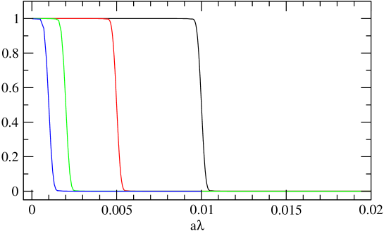
Figure 1: Approximate step function for the lowest bin $a\lambda=[0,a\delta]$. The cases of $a\delta$ = 0.01, 0.005, 0.002 and 0.001 are plotted. The degree of polynomial is $p$ = 8000.

Examples of the filtering function are shown in Figure 1 for the order of polynomial $p$ = 8000. Here, the Dirac eigenvalue $a\lambda$ as defined in (13) is taken on the horizontal axis. The plot shows the function to extract the count in the lowest bin $[0,a\delta]$ of bin size $a\delta$ = 0.01, 0.005, 0.002 and 0.001. The approximation of the step function is very precise except for the region close to the threshold $a\lambda=a\delta$. The width where the function varies is nearly independent of $a\delta$, and as a result, the relative error of the approximation is smaller for larger bin sizes. Note that the lowest eigenvalue is the worst case, because it is mapped onto a narrow bin of size $2(a\delta)^{2}$ of $A$.

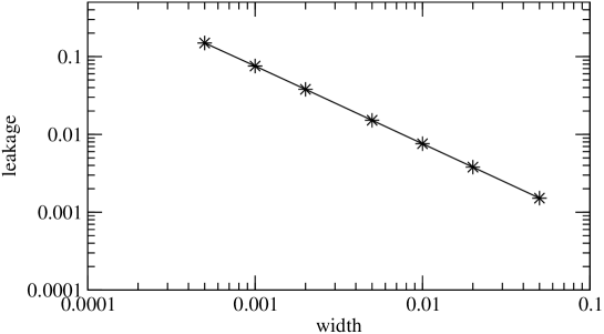
Figure 2: Fractional leakage from the lowest bin $\lambda=[0,\delta]$ to the neighboring bin. The fraction of the leakage is plotted as a function of the bin size $a\delta$. The case of $p$ = 8000 is plotted.

In order to quantify the size of the error in filtering, we calculate a fraction of leakage from the lowest bin $[0,a\delta]$ to the neighboring bin. It is defined as an integral of the filtering function from $a\delta$ to infinity, which should vanish for the exact step function. The leakage is equal to the deficit in the bin of interest $[0,a\delta]$. Figure 2 shows the leakage for various widths $a\delta$. The relative error increases for smaller $a\delta$ as an inverse power $1/a\delta$. If we allow an 1% error for the calculation of the spectral function, we may take $a\delta$ to be 0.005 when $p$ = 8000. This bin size corresponds to 12 MeV on our coarsest lattice. On finer lattices we take larger values of $p$ so that the error with a fixed $\delta$, which implies a smaller $a\delta$ on a finer lattice, is not larger than 0.005. Since the deficit is largely compensated by the leakage from the neighboring bin when the spectral function is nearly constant as it is the case for zero temperature QCD, the actual error would be much smaller than this naive estimate.

According to the general theory of the Chebyshev approximation, the error as measured by the $L_{2}$ norm scales as $1/\sqrt{p}$ DiNapole:2013 . With the Jackson damping factor implemented in this work, this bound does not apply, but an actual calculation as outlined above indicates that the leakage decreases as $1/p$. This determines the computational cost when one wants to improve the precision using this method.

4 Lattice ensembles

$\beta$	$a^{-}1$	$L/a$	$am_{ud}$	$am_{s}$	$m_{\pi}$	$p$	$N_{meas}$
	[GeV]				[MeV]
4.17	2.453(4)	32	0.019	0.030	498.0(0.7)	8,000	100
			0.012		396.8(0.7)		100
			0.007		309.8(1.0)		100
			0.019	0.040	498.7(0.7)	8,000	100
			0.012		399.0(0.8)		100
			0.007		309.2(1.0)		100
			0.0035		229.8(1.1)		100
		48	$\uparrow$		225.8(0.3)	9,000	100
4.35	3.610(9)	48	0.0120	0.0180	498.5(0.9)	16,000	50
			0.0080		407.0(1.2)		50
			0.0042		295.9(1.2)		50
			0.0120	0.0250	500.7(1.0)	16,000	50
			0.0080		407.8(1.0)		50
			0.0042		299.9(1.2)		50
4.47	4.496(9)	64	0.0030	0.0150	284.2(0.7)	15,000	40

Table 1: Lattice ensembles used in the eigenvalue spectrum calculation. Spatial lattice size $L/a$ and sea quark masses $am_{ud}$, $am_{s}$ are listed in the lattice unit. $p$ is the order of the Chebyshev polynomial, and $N_{meas}$ is the number of measurements. Empty entries are the same as the ones in the previous line.

We calculate the spectral function at three $\beta$ values on 15 gauge ensembles in total, generated with 2+1 flavors of sea quarks Noaki:2014sda , as listed in Table 1. The formulation for the sea quarks is the Möbius domain-wall fermion, which is the same for the lattice Dirac operator used in the eigenvalue counting. The gauge action is tree-level Symanzik improved, and we apply the stout link smearing Morningstar:2003gk three times for the link variables entering the definition of the fermionic operators.

The lattice spacings determined through the Wilson flow scale $t_{0}$ are 0.0803(1), 0.0546(1) and 0.0438(1) fm at $\beta$ = 4.17, 4.35, 4.47, respectively, where we report only the statistical error. We chose the input $t_{0}^{1/2}$ = 0.1465(21)(13) fm from Borsanyi:2012zs . The error on this input value is taken into account as one of the sources of systematic error.

Except for the finest lattice ($\beta$ = 4.47), we generated lattices at several values of $(am_{ud},am_{s})$, combinations of the up/down and strange quark masses. Corresponding pion mass $m_{\pi}$ covers the range between 230 and 500 MeV. Two strange quark masses sandwich its physical value. The finest lattice at $\beta$ = 4.47 is available only at one combination of sea quark masses. The corresponding pion mass is about 280 MeV.

The spatial extent of the lattice $L/a$ is chosen such that the physical size $L$ is kept constant around 2.6–2.8 fm. The measure of the finite volume effect $m_{\pi}L$ is larger than 3.9 for all ensembles except for the one of the lightest sea quark mass ($am_{ud}$ = 0.0035) on the $L/a=32$ lattice. For this parameter we prepare a lattice ensemble of larger volume, $L/a=48$, in order to examine the finite volume effect. On this larger lattice, $m_{\pi}L$ = 4.4. The results from the $L/a=32$ lattice at this parameter are used only to investigate the finite volume effect and not included in the final analysis of the chiral condensate. The temporal size $T$ is always twice as large as the spatial size $L$.

For each ensemble we run a Hybrid Monte Carlo simulation for 10,000 molecular-dynamics trajectories, out of which we chose (equally separated) $N_{meas}$ = 40–100 gauge configurations for the calculation of the spectral function.

The Möbius domain-wall fermion is defined on a 5D lattice. The extent in the fifth dimension $L_{s}$ is chosen such that the violation of the Ginsparg-Wilson relation is sufficiently small. By taking $L_{s}$ = 12 on the coarsest lattice at $\beta$ = 4.17 we confirm that the residual mass is roughly 1 MeV Hashimoto:2014gta . On the finer lattices at $\beta$ = 4.35 and 4.47, we take $L_{s}$ = 8 and the residual mass is much smaller: 0.2 MeV at $\beta$ = 4.35 and $<0.1$ MeV at $\beta$ = 4.47. These small but non-zero residual mass may distort the low-lying Dirac spectrum. With the bin size we chose to count the eigenvalues, such effect would be minor; we eventually eliminate the associated error by taking the continuum limit using the three lattice spacings we prepared.

The same set of ensembles is used for a wide variety of applications including a determination of non-perturbative renormalization constant Tomii:2016xiv , a determination of the charm quark mass from temporal moments of charmonium correlator Nakayama:2016atf , a calculation of the $\eta^{\prime}$ meson mass through a gluonic observable Fukaya:2015ara , and a calculation of $D_{(s)}$ meson decay constant Fahy:2015xka . Numerical calculations of the projects are performed using the code set IroIro++ Cossu:2013ola .

5 Spectral function: overview

First, we demonstrate how the eigenvalue filtering method works by showing the results on our coarsest lattices, i.e. $32^{3}\times 64$ lattices at $\beta=4.17$. The sea quark masses are $(am_{ud},am_{s})$ = (0.0035,0.040), (0.007, 0.040), (0.012, 0.040), (0.019, 0.040). The corresponding pion mass ranges between 230 MeV and 500 MeV.

Averaging over 50 gauge configurations each with only one noise per configuration, we calculated $\langle\xi_{k}^{\dagger}T_{j}(A)\xi_{k}\rangle$. The mode number $\bar{n}[s,t]$ is then evaluated by summing over $j$ from 0 to $p$ as (6). The spectral density is obtained with an appropriate normalization,

$$a^{3}\rho(\lambda;\delta)=\frac{1}{2V/a^{4}}\frac{\bar{n}[s,t]}{a\delta},$$ (14)

where $a\lambda=s^{1/2}/(1-s)$ and $a(\lambda+\delta)=t^{1/2}/(1-t)$. The factor 2 in the denominator of (14) reflects the pairing of the eigenvalues, i.e. $\pm i\lambda$.

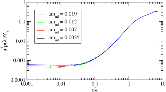
Figure 3: Spectral function in the entire range of $a\lambda$. Both the horizontal and vertical axes are logarithmic. Data obtained at $\beta$ = 4.17 at four values of light quark mass $am_{ud}$.

Figure 3 shows the spectral density $a^{3}\rho(\lambda)$ in the whole range of $a\lambda$. The bin size is $a\delta$ = 0.005. One can clearly observe that the spectrum starts from a tiny constant at $\lambda\simeq 0$ and increases towards higher eigenvalues. The near-zero modes show some dependence on the sea quark mass (see below), but the high modes are nearly independent of the sea quark mass.

The increase towards the perturbative regime at high $a\lambda$ is qualitatively consistent with the free-theory scaling $\sim\lambda^{3}$, but saturates at around $a\lambda\sim 1$ due to the discretization effect.

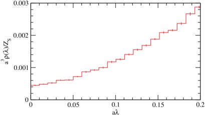
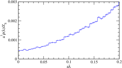
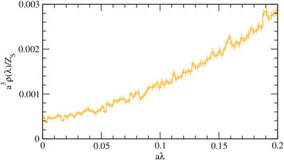
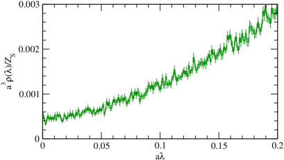
Figure 4: Spectral function in the low-lying region. The data at $\beta=4.17$ and $(am_{ud},am_{s})$ = (0.007, 0.030). Results with different bin sizes are shown: $a\delta$ = 0.01, 0.005, 0.002, and 0.001 from top left to bottom right.

Figure 4 shows the spectral function in the low-lying regime. The data at $(am_{ud},am_{s})$ = (0.007, 0.030) are shown. Results of different bin sizes ($a\delta$ = 0.01, 0.005, 0.002, 0.001) are plotted. We find that they are consistent within the statistical errors. The statistical error is larger for smaller bins since the number of eigenvalues in each bin is fewer.

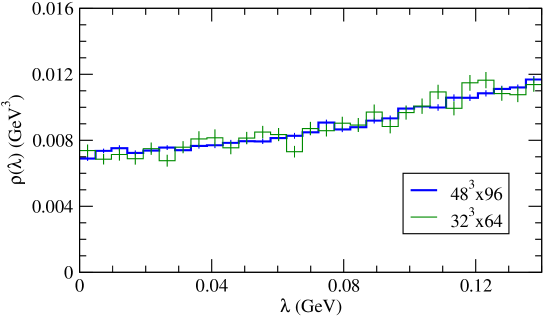
Figure 5: Volume scaling of the spectral function $\rho(\lambda)$. The data on the coarsest lattice ($\beta$ = 4.17) at two different volumes $48^{3}\times 96$ (thick line) and $32^{3}\times 64$ (thin) at $am_{ud}$ = 0.0035 and $am_{s}$ = 0.040.

The volume scaling of the spectral function is demonstrated in Figure 5. For the lightest pion ($m_{\pi}\simeq$ 230 MeV), there are data on two volumes $32^{3}\times 64$ and $48^{3}\times 96$ available. We calculate the spectral density on both lattices with exactly the same method. The results are consistent with each other within the statistical error, which is about 5% on the $32^{3}\times 64$ lattice. The statistical error is smaller, about 2%, on the larger volume since the number of eigenvalues in a given bin is proportional to the physical volume $V$.

6 Analysis with chiral perturbation theory

The Banks-Casher relation $\rho(0)=\Sigma/\pi$ is valid only in the chiral limit after taking the infinite volume limit. Therefore, the effects of finite sea quark masses and finite volume need to be taken into account in the analysis. We use the functional form predicted by the chiral effective theory to analyze the quark mass dependence. The finite volume effect is also estimated within the same framework, but it turned out to be negligible in our setup as discussed below.

The analytic calculation is available at the one-loop order of chiral perturbation theory ($\chi$PT), which is valid at the leading non-trivial order of finite quark mass correction, i.e. of order $m_{\pi}^{2}/(4\pi F_{\pi})^{2}$. The formula is concisely written in the form Damgaard:2008zs (see also Fukaya:2010na )

$$\rho(\lambda)=\frac{\Sigma}{\pi}\left[1-\frac{1}{F^{2}}\left(\sum_{i}\mathrm{Re}\Delta(0,M_{vi}^{2})-\mathrm{Re}G(0,M_{vv}^{2},M_{vv}^{2})-16L_{6}\sum_{i}M_{ii}^{2}\right)\right]_{m_{v}=i\lambda},$$ (15)

where the chiral condensate $\Sigma$ and pion decay constant $F$ are those in the chiral limit. One of the low-energy constants at the one-loop order, $L_{6}$, appears for this quantity. The functions $\Delta(0,M^{2})$ and $G(0,M^{2},M^{2})$ are given as

$$\Delta(0,M^{2}) = \frac{M^{2}}{16\pi^{2}}\ln\frac{M^{2}}{\mu_{sub}^{2}}+g_{1}(M^{2}),$$ (16)

$$G(0,M^{2},M^{2}) = \frac{1}{2}\left[\Delta(0,M^{2})+(M^{2}-M_{\pi}^{2})\partial_{M^{2}}\Delta(0,M^{2})\right].$$ (17)

They are evaluated at a “pion mass” as determined by the Gell-Mann-Oakes-Renner (GMOR) relation $M_{ij}^{2}=(m_{i}+m_{j})\Sigma/F^{2}$, where the indices $i$ and $j$ label the sea quark mass or a fictitious valence quark $v$. For the sea quark mass, it gives a leading-order estimate of the corresponding pion mass. It slightly deviates from the actual pion mass calculated on the lattice with the same quark mass, but the difference is from higher orders of the chiral expansion and thus can be neglected at the order considered for $\rho(\lambda)$. The “valence quark” mass $m_{v}$ is taken at an imaginary value $i\lambda$ to obtain the spectral function $\rho(\lambda)$ at a finite $\lambda$, according to the procedure in Damgaard:2008zs . The scale parameter $\mu_{sub}$ denotes the renormalization scale, which is conventionally taken at the $\rho$ meson mass.

The function $g_{1}(M^{2})$ in (16) represents the finite volume effect and is written in terms of a sum of the modified Bessel function. In the analysis of chiral extrapolation, we ignore the contribution of $g_{1}(M^{2})$, which is a good approximation for our data. The largest possible finite volume effect may arise for the ensemble of lightest pion with the smaller volume, i.e. the $32^{3}\times 64$ lattice of $am_{ud}=0.0035$ at $\beta=4.17$, for which our estimate of $g_{1}(M^{2})/F^{2}$ is $\sim$0.05 (0.02) at $\lambda\simeq$ 5 MeV (10 MeV). The maximum finite volume effect appears for smaller $\lambda$. Even for this maximum case, the expected error due to neglecting such effects is about the same size as the statistical error. For the analysis of chiral extrapolation, we mainly use a larger bin of size 15 MeV, for which the estimated finite volume effect is well below the statistical error.

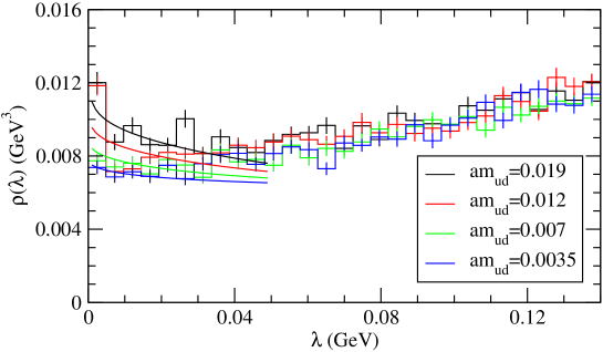
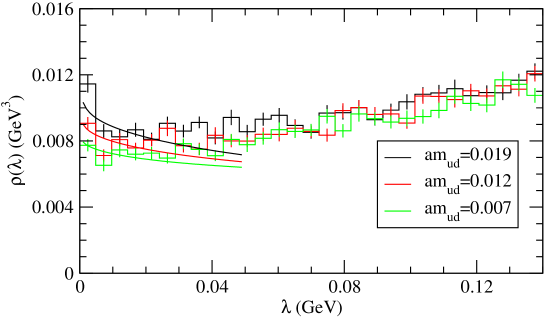
Figure 6: Dirac spectrum in the low-lying region. The data on the coarsest lattice ($\beta$ = 4.17) at two different strange quark masses: $am_{s}$ = 0.040 (top) and 0.030 (bottom). Results at $am_{ud}$ = 0.019 (black), 0.012 (red), 0.007 (green), 0.0035 (blue) are plotted. Curves are from chiral perturbation theory. See text for details.

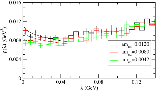
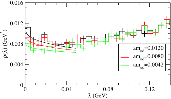
Figure 7: Dirac spectrum in the low-lying region. The data on the mid-fine lattice ($\beta$ = 4.35) at two different strange quark masses: $am_{s}$ = 0.025 (top) and 0.018 (bottom). Results at $am_{ud}$ = 0.0120 (black), 0.0080 (red), and 0.0045 (green) are plotted. Curves are from chiral perturbation theory. See text for details.

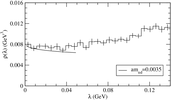
Figure 8: Dirac spectrum in the low-lying region. The data on the finest lattice ($\beta$ = 4.47) at $am_{ud}$ = 0.0035 and $am_{s}$ = 0.0150 (black) are plotted. Curves are from chiral perturbation theory. See text for details.

In Figures 6–8 we compare the lattice results with those of $N_{f}=2$ $\chi$PT at one-loop. The plots for each $\beta$ and strange quark mass are shown in separate panels. The lattice data are renormalized with the renormalization factor for the scalar-density operator calculated separately using the short-distance current correlator Tomii:2016xiv . The renormalization scheme is that of the $\overline{\mbox{MS}}$ scheme at the scale of 2 GeV. The values are $Z_{S}(\mathrm{2~{}GeV})$ = 1.037(15), 0.934(9), and 0.893(7), for $\beta$ = 4.17, 4.35, and 4.47, respectively.

From the data we can see a clear dependence on the up-down quark mass near $\lambda=0$. In $\chi$PT, the quark mass dependence is induced at the one-loop order through the functions $\Delta(0,M^{2})$ and $G(0,M^{2},M^{2})$ as well as through the counter term including $L_{6}$. Another prominent feature of the low-mode spectrum $\rho(\lambda)$ is the increase below $\lambda\sim$ 20 MeV, which is more pronounced for heavier sea quarks, while the rise almost disappears at the lightest up and down sea quarks available at $\beta$ = 4.17 (upper panel of Figure 6).

The one-loop $\chi$PT prediction of $N_{f}=2$ is shown by curves in Figures 6–8. The curves are for $\Sigma^{1/3}(\mathrm{2~{}GeV})$ = 270 MeV and $L_{6}$ = 0.0030, which are the central values of a fit (see below) with a nominal value of $F$ = 90 MeV. The strange quark mass dependence is introduced assuming a linear dependence of $\Sigma^{1/3}(\mathrm{2~{}GeV})$ on $m_{s}$. The value of $\Sigma^{1/3}(\mathrm{2~{}GeV})$ mentioned is at the physical strange quark mass.

Figures 6–8 demonstrate that the $\chi$PT curves also show the increase toward $\lambda=0$ especially for heavier sea quarks and nicely reproduce the lattice data, which show the increase below $\lambda\sim$ 15–20 MeV. This is not due to a tuning of parameters. In fact, the extra parameter $L_{6}$ appearing at the one-loop order controls only the overall shift of $\rho(\lambda)$ without influencing its $\lambda$ dependence. The functional form of the pion-loop contribution, $\mathrm{Re}\Delta(0,M_{vi}^{2})$ and $\mathrm{Re}G(0,M_{vv}^{2},M_{vv}^{2})$, is responsible for the increase toward $\lambda$ = 0. On the other hand, the one-loop $\chi$PT formula does not explain the slight growth toward larger $\lambda$ above $\lambda\sim$ 20 MeV. The higher order calculations would be needed to describe this regime.

With the $N_{f}=3$ $\chi$PT in which kaons and $\eta$ are also taken as the dynamical degrees of freedom of chiral effective theory, the number of parameters is reduced as we do not need to separately model the strange quark mass dependence. It turned out that a formula including $\Sigma^{1/3}(\mathrm{2~{}GeV})$, $L_{6}$ and a parameter to describe the discretization effect as fit parameters does not fit the data well. ($\chi^{2}$/dof is larger than 3.5.) It is probably due to too large strange quark mass to be treated within the $\chi$PT framework. In fact, our data for $\rho(\lambda)$ deviates from the one-loop $\chi$PT results above $\lambda\simeq$ 20 MeV. The physical strange quark mass 90–100 MeV is far beyond this threshold.

We determine the parameters $\Sigma$ and $L_{6}$ through a fit of the lattice data while fixing $F$ = 90 MeV. The fit is done for the value of

$$\bar{\rho}[0:\delta]=\frac{1}{\delta}\int_{0}^{\delta}d\lambda\rho(\lambda)$$ (18)

with $\delta$ = 0.015 GeV. Both the lattice data and the $\chi$PT formula are integrated in the region $[0,\delta]$. This value of $\delta$ corresponds to $2\delta\Sigma/F^{2}\simeq$ 250 MeV, which is well below the kaon mass. It corresponds to the lowest three bins in the plots shown in Figures 6–8. In this region, the $\chi$PT formula describes the data quite well.

The strange quark mass dependence of $\rho(\lambda)$ is introduced assuming a linear dependence of $\rho(\lambda)$ on $m_{s}$. In the narrow range of the strange quark quark mass adopted in our simulation and with the mild dependence of $\rho(\lambda)$ on $m_{s}$, this approximation should describe the data well. Namely, we multiply

$$1+c_{s}(M_{\eta_{ss}}^{2}-M_{\eta_{ss}}^{\mathrm{(phys)}2})$$ (19)

as an overall factor to $\rho(\lambda)$ in (15) to interpolate the data to the physical strange quark mass. The parameter $c_{s}$ is to be determined by a fit. Here, $M_{\eta_{ss}}^{\mathrm{(phys)}}$ = 687 MeV is a mass of fictitious $s\bar{s}$ pseudo-scalar meson estimated using the GMOR relation. Our lattice ensembles contain those of different strange quark masses while other parameters are fixed. The strange quark masses in the simulations are chosen in such a way that they sandwich its physical value. We in effect interpolate between them by (19).

Similarly, the discretization effect is parameterized by a linear function in $a^{2}$, multiplying $1+c_{a}a^{2}$ as an overall factor with $c_{a}$ a fit parameter.

The fit for the all available data points yield $\Sigma^{1/3}(\mathrm{2~{}GeV})$ = 270.0(1.3) MeV, $L_{6}$ = 0.00016(6), as well as $c_{s}$ = 0.50(30) GeV^-2, $c_{a}$ = 0.00(15) GeV², with $\chi^{2}/\mathrm{dof}$ = 1.29. As advertised, the discretization effect is invisible within the statistical error.

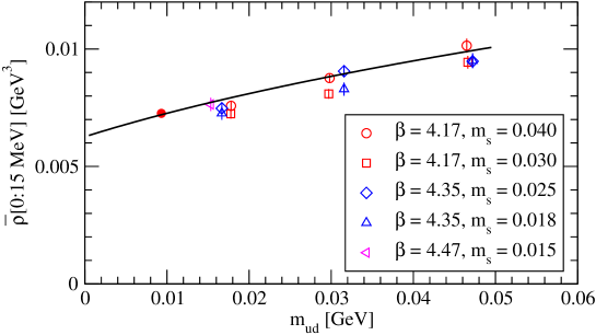
Figure 9: Chiral extrapolation of $\bar{\rho}[0:\delta]$. Data are averaged in the lowest bin of $\delta$ = 15 MeV. Open symbols are lattice data from each ensemble. Different symbols correspond to different lattice spacings and strange quark masses, as denoted in the inset. A filled circle near $m_{ud}$ = 0.01 GeV is that of lightest quark at $\beta$ = 4.17 and $am_{s}$ = 0.040 on the larger volume $48^{3}\times 96$. Data are plotted against the up-down quark mass $m_{ud}$ renormalized with the $\overline{\mathrm{MS}}$ scheme at a scale 2 GeV. The solid curve is that of the one-loop $\chi$PT fit in the continuum limit and at the physical strange quark mass.

Chiral extrapolation of $\bar{\rho}[0:\delta]$ is shown in Figure 9 as a function of sea up and down quark mass $m_{ud}$. Data points do not lie on a single universal curve because the data at different strange quark masses are put in the same plot. In other words, there is a significant strange quark mass dependence, which seems to be well described by an overall shift of the curve. Dependence on the lattice spacing is not very significant from the plot, as the fit also suggests. The curvature due to the one-loop correction is not strong but still visible, and makes the chiral limit slightly lower than a naive linear extrapolation in $m_{ud}$.

We list the possible sources of systematic errors in the following. First of all, the renormalization constant $Z_{S}(\mathrm{2~{}GeV})$ determined in Tomii:2016xiv contains some errors. (The numbers are given above.) The size is 1.4%, 1.0% and 0.8% for coarse, medium and fine lattices, respectively. We take the largest error, 1.4%, to be conservative, for the estimate of the error for $\Sigma(\mathrm{2~{}GeV})$. When we quote the number for $\Sigma^{1/3}(\mathrm{2~{}GeV})$, we therefore assign 0.5% as an estimated systematic error from this source.

The discretization effect is well under control in our calculation. In fact, our fit implies that the lattice-spacing dependence is consistent with zero. Although it is insignificant, by keeping the term describing this effect in the fit function, we can take account of possible systematic effect. We therefore do not add extra errors from the discretization effects.

Finite volume effect is explicitly checked on the ensembles with the lightest pion ($\sim$ 230 MeV) as shown in Figure 5. We do not observe any statistically significant difference between the two volumes ($32^{3}$ and $48^{3}$), which is consistent with an expectation from $\chi$PT, i.e. the predicted size of the finite volume effect is about 5% for the smaller lattice and is about the same size as the statistical error. For heavier pions the $\chi$PT predicts exponentially suppressed finite volume effects. Therefore, for all the data used in the fit to extract the chiral condensate, this source of error is within our statistical error. (Note that the smaller volume data at $M_{\pi}\sim$ 230 MeV are not included in the fit.)

Higher-order corrections from $\chi$PT may be significant especially for larger $\lambda$ and heavier quarks. Since we can explicitly confirm the consistency of the lattice data with the one-loop $\chi$PT for its $\lambda$-dependence in the range of our analysis, we expect that two-loop correction is insignificant below $\lambda$ = 15 MeV. We checked that the result with a slightly smaller bin size, 10 MeV, is consistent within the statistical error. Also for the quark mass, the one-loop $\chi$PT fits the lattice data well up to the data points of heaviest pion masses ($\sim$ 500 MeV). In order to examine the significance of the higher order effects, we tried to fit the data with a function including the analytic terms of $O(M^{4}/F^{4})$. The coefficient obtained from such an analysis is of order of $3\times 10^{-6}$ and statistically consistent with zero. The best fit value of $\Sigma^{1/3}(\mathrm{2~{}GeV})$ is shifted by only 0.1 MeV, which is much smaller than the statistical error. We can conclude that such effects are well below the statistical error in our analysis.

There is a potential effect of slightly inaccurate implementation of the Ginsparg-Wilson relation with the Möbius domain-wall fermion. As we already discussed, the 4D effective operator of the Möbius domain-wall fermion violates the Ginsparg-Wilson relation by the amount characterized by the residual mass, which is about 1 MeV on our coarsest lattice and an order of magnitude smaller on finer lattices. It means that the eigenvalue of the Dirac operator is distorted by the amount of $O(\mathrm{1~{}MeV})$ on the lattices at $\beta$ = 4.17. Since the bin size in the analysis is much larger (= 15 MeV), the error due to this effect is minor. Moreover, the effect should be negligible on finer lattices, and it is also taken into account by the continuum extrapolation. We therefore do not introduce additional error budget for this effect.

Finally, our input value for lattice spacing has an error of 1.7%, which affects dimensionful quantities, including the chiral condensate. We therefore add this size of error for $\Sigma^{1/3}$.

Having these various systematic errors considered, we quote

$$\Sigma^{1/3}(\mathrm{2~{}GeV})=\mbox{270.0(1.3)(1.3)(4.6)~{}MeV},$$ (20)

where the errors are those from statistical, renormalization, and lattice scale, respectively. Adding in quadrature, the total error is 4.9 MeV, which is 1.8%. The Flavour Lattice Averaging Group (FLAG) quotes the chiral condensate for $N_{f}$ = 2+1, $\Sigma^{1/3}(\mathrm{2~{}GeV})$ = 274(3) MeV Aoki:2016frl , as an average of Blum:2014tka ; Bazavov:2010yq ; Borsanyi:2012zv ; Durr:2013goa . They are obtained by fitting meson masses and decay constants with the $\chi$PT formulae, where the chiral condensate appears as a coefficient in the Gell-Mann-Oakes-Renner (GMOR) relation. Our result (20) is consistent with the world average and the precision is comparable.

7 Conclusion

The eigenvalue spectrum of the Dirac operator reflects the quantum effects of QCD. The near-zero eigenvalue regime is special, as it can be connected to the order parameter of spontaneous chiral symmetry breaking in QCD, i.e. the chiral condensate. This relation known as the Banks-Casher relation can be extended to the case of finite $\lambda$ as well as finite quark masses using $\chi$PT. This work provides a direct test of these relations by calculating the spectral function in lattice QCD simulations.

The Möbius domain-wall fermion formulation used in this work to define the Dirac operator possesses an approximate chiral symmetry with an error of order 1 MeV at most, and the accumulation of the eigenvalues above this value is not much affected by this artifact. We extract the chiral condensate from the spectrum below 15 MeV by fitting the lattice data with the $\chi$PT formula. The discretization error is well under control and even extrapolated away to the continuum limit using relatively fine-grained lattices of $a$ = 0.080–0.044 fm.

The remaining uncertainty is at the level of 2% for $\Sigma^{1/3}(\mathrm{2~{}GeV)}$. This provides a precise test of the GMOR relation, since there is no free parameter left for the leading-order equation $m_{\pi}^{2}/m=2\Sigma/F^{2}$ once $m_{\pi}$ and $F$ are calculated. The agreement of our result 270.0(4.9) MeV with that of an average of previous results obtained through GMOR gives further evidence supporting $\chi$PT as an effective theory of QCD at low energies.

The eigenvalue filtering technique utilized in this work is proven to be effective to obtain the spectral function of the Dirac operator. In this analysis we used only the near-zero regime of the eigenvalues, while the entire spectrum is calculated as a by-product. Such information may be useful to extract the mass anomalous dimension of QCD with a non-perturbative method as discussed in Fodor:2016hke .

References

- (1) T. Banks and A. Casher, Nucl. Phys. B 169 (1980) 103. doi:10.1016/0550-3213(80)90255-2
- (2) A. V. Smilga and J. Stern, Phys. Lett. B 318, 531 (1993). doi:10.1016/0370-2693(93)91551-W
- (3) J. C. Osborn, D. Toublan and J. J. M. Verbaarschot, Nucl. Phys. B 540, 317 (1999) doi:10.1016/S0550-3213(98)00716-0 [hep-th/9806110].
- (4) G. Akemann, arXiv:1603.06011 [math-ph].
- (5) P. H. Damgaard and H. Fukaya, JHEP 0901, 052 (2009) [arXiv:0812.2797 [hep-lat]].
- (6) L. Giusti and M. Luscher, JHEP 0903, 013 (2009) [arXiv:0812.3638 [hep-lat]].
- (7) H. Fukaya et al. [JLQCD Collaboration], Phys. Rev. Lett. 98, 172001 (2007) doi:10.1103/PhysRevLett.98.172001 [hep-lat/0702003].
- (8) H. Fukaya et al. [TWQCD Collaboration], Phys. Rev. D 76, 054503 (2007) doi:10.1103/PhysRevD.76.054503 [arXiv:0705.3322 [hep-lat]].
- (9) H. Fukaya et al. [JLQCD Collaboration], Phys. Rev. Lett. 104, 122002 (2010) Erratum: [Phys. Rev. Lett. 105, 159901 (2010)] doi:10.1103/PhysRevLett.104.122002, 10.1103/PhysRevLett.105.159901 [arXiv:0911.5555 [hep-lat]].
- (10) H. Fukaya et al. [JLQCD and TWQCD Collaborations], Phys. Rev. D 83, 074501 (2011) doi:10.1103/PhysRevD.83.074501 [arXiv:1012.4052 [hep-lat]].
- (11) P. H. Damgaard and S. M. Nishigaki, Nucl. Phys. B 518, 495 (1998) doi:10.1016/S0550-3213(98)00123-0 [hep-th/9711023].
- (12) P. H. Damgaard and S. M. Nishigaki, Phys. Rev. D 63, 045012 (2001) doi:10.1103/PhysRevD.63.045012 [hep-th/0006111].
- (13) G. P. Engel, L. Giusti, S. Lottini and R. Sommer, Phys. Rev. Lett. 114, no. 11, 112001 (2015) doi:10.1103/PhysRevLett.114.112001 [arXiv:1406.4987 [hep-ph]].
- (14) G. P. Engel, L. Giusti, S. Lottini and R. Sommer, Phys. Rev. D 91, no. 5, 054505 (2015) doi:10.1103/PhysRevD.91.054505 [arXiv:1411.6386 [hep-lat]].
- (15) K. Cichy, E. Garcia-Ramos and K. Jansen, JHEP 1310, 175 (2013) doi:10.1007/JHEP10(2013)175 [arXiv:1303.1954 [hep-lat]].
- (16) E. Di Napoli, E. Polizzi and Y. Saad, arXiv:1308.4275 [cs.NA].
- (17) P. H. Ginsparg and K. G. Wilson, Phys. Rev. D 25, 2649 (1982). doi:10.1103/PhysRevD.25.2649
- (18) G. Cossu, H. Fukaya, S. Hashimoto, T. Kaneko and J. Noaki, arXiv:1601.00744 [hep-lat].
- (19) Z. Fodor, K. Holland, J. Kuti, S. Mondal, D. Nogradi and C. H. Wong, arXiv:1605.08091 [hep-lat].
- (20) R. C. Brower, H. Neff and K. Orginos, arXiv:1206.5214 [hep-lat].
- (21) D. B. Kaplan, Phys. Lett. B 288, 342 (1992) doi:10.1016/0370-2693(92)91112-M [hep-lat/9206013].
- (22) Y. Shamir, Nucl. Phys. B 406, 90 (1993) doi:10.1016/0550-3213(93)90162-I [hep-lat/9303005].
- (23) J. Noaki et al. [JLQCD Collaboration], PoS LATTICE 2014, 069 (2014).
- (24) C. Morningstar and M. J. Peardon, Phys. Rev. D 69, 054501 (2004) doi:10.1103/PhysRevD.69.054501 [hep-lat/0311018].
- (25) S. Borsanyi et al., JHEP 1209, 010 (2012) doi:10.1007/JHEP09(2012)010 [arXiv:1203.4469 [hep-lat]].
- (26) S. Hashimoto, S. Aoki, G. Cossu, H. Fukaya, T. Kaneko, J. Noaki and P. A. Boyle, PoS LATTICE 2013, 431 (2014).
- (27) M. Tomii et al. [JLQCD Collaboration], arXiv:1604.08702 [hep-lat].
- (28) K. Nakayama, B. Fahy and S. Hashimoto, arXiv:1606.01002 [hep-lat].
- (29) H. Fukaya et al. [JLQCD Collaboration], Phys. Rev. D 92, no. 11, 111501 (2015) doi:10.1103/PhysRevD.92.111501 [arXiv:1509.00944 [hep-lat]].
- (30) B. Fahy, G. Cossu, S. Hashimoto, T. Kaneko, J. Noaki and M. Tomii, arXiv:1512.08599 [hep-lat].
- (31) G. Cossu, J. Noaki, S. Hashimoto, T. Kaneko, H. Fukaya, P. A. Boyle and J. Doi, arXiv:1311.0084 [hep-lat].
- (32) S. Aoki et al., arXiv:1607.00299 [hep-lat].
- (33) T. Blum et al. [RBC and UKQCD Collaborations], Phys. Rev. D 93, no. 7, 074505 (2016) doi:10.1103/PhysRevD.93.074505 [arXiv:1411.7017 [hep-lat]].
- (34) A. Bazavov et al., PoS LATTICE 2010, 083 (2010) [arXiv:1011.1792 [hep-lat]].
- (35) S. Borsanyi, S. Durr, Z. Fodor, S. Krieg, A. Schafer, E. E. Scholz and K. K. Szabo, Phys. Rev. D 88, 014513 (2013) doi:10.1103/PhysRevD.88.014513 [arXiv:1205.0788 [hep-lat]].
- (36) S. Dürr et al. [Budapest-Marseille-Wuppertal Collaboration], Phys. Rev. D 90, no. 11, 114504 (2014) doi:10.1103/PhysRevD.90.114504 [arXiv:1310.3626 [hep-lat]].