Using the PPML approach for constructing a low-dissipation, operator-splitting scheme for numerical simulations of hydrodynamic flows

Abstract

An approach for constructing a low-dissipation numerical method is described. The method is based on a combination of the operator-splitting method, Godunov method, and piecewise-parabolic method on the local stencil. Numerical method was tested on a standard suite of hydrodynamic test problems. In addition, the performance of the method is demonstrated on a global test problem showing the development of a spiral structure in a gravitationally unstable gaseous galactic disk.

1 INTRODUCTION

During the last two decades, two main approaches have been used for numeral hydrodynamics simulations of astrophysical flows: the Lagrangian smooth particle hydrodynamics methods (hereafter, the SPH method) and Eulerian mesh-based methods. Numerous comparisons between the SPH and mesh-based methods have been performed [1, 2]. The main disadvantages of most SPH methods are the inaccurate computation of large gradients and discontinuities [3], suppression of physical instabilities [1], difficulty with choosing the proper smoothing kernel [4] and the use of artificial viscosity [5]. The main disadvantages of most mesh-based methods are their Galilean non-invariance on the mesh [2, 6], difficulty with coding and implementation, and difficulty with treating multi-component systems, such as stars and gas [7]. During the last decade, the combined Eulerian-Lagrangian approach has been developed and actively used for numerical simulations of astrophysical hydrodynamics flows [8, 9]. These methods unite the advantages of both approaches, while attempting to reduce the disadvantages.

Recently, another Eulerian-Lagrangian numerical scheme for astrophysical flows has been presented, which employs the operator-splitting methodology and Godunov-type methods [3, 10, 11, 12, 13]. This numerical method is based on the solution of hydrodynamic equations in two stages. At the first Eulerian step, the hydrodynamic equations are solved excluding the advective terms. At the second Lagrangian step, equations for the advective transport are solved. This separation into two stages can effectively solve the problem of Galilean-invariance and the use of Godunov methods for the Eulerian step enables correct modelling of discontinuous solutions. This numerical method has been successfully employed for modeling collisions between galaxies [12, 14]. A significant disadvantage of the method lays in the fact that it was first-order accurate. The main shortcoming of first-order schemes is dissipation of the numerical solution on discontinuities. It is therefore our main motivation to extend the original method to a higher order of accuracy.

There are several well-known high-order numerical hydrodynamics methods such as the MUSCL (Monotonic Upstream-Centered Scheme for Conservation Laws) method [15, 16], total variation diminishing (TVD) method [17, 18, 19, 20, 21], and piecewise parabolic method (PPM) [22]. The general idea of their approach is the construction of a piecewise-polynomial function on each cell of the numerical mesh. It may be a piecewise-linear reconstruction (in the case of the MUSCL scheme) or piecewise-parabolic reconstruction (in the case of the PPM method). For the construction of a monotonized numerical solution (needed to avoid the growth of spurious extrema) the limiters are usually employed in TVD methods [23]. The problem of selection of limiters is analogous to the choice of artificial viscosity in SPH methods: the wrong choice of artificial viscosity for the SPH method (or limiters for the TVD method) can cause a substantial distortion of the numerical solution. The PPM method does not have the monotonicity problem, because piecewise-polynomial solutions on each cell are constructed without extrema. The main disadvantage of the PPM method is the use of a non-local stencil for computing hydrodynamic quantities on the next time step. The non-local stencil has problems with the proper choice of boundary conditions, domain decomposition, and dissipation of numerical solution. To resolve these problems, a modification of the PPM method was suggested – the so-called piecewise-parabolic method on the local stencil (PPML) [24, 25]. The main idea of the PPML method is the use of a piecewise parabolic numerical solution on the previous time step for computing the Riemann problem.

Numerical simulations of galaxies are an indispensable tool for studying their properties and evolution, taking into account the complexity of physical processes involved. The main galactic components such as gas and dust can be modelled as fluids, making numerical hydrodynamics simulations the main numerical approach. The main focus of this paper is concentrated on the extension of the original method [3, 10, 11, 12, 13] based on the PPML approach to a higher order of accuracy. The methods presented here are specific to astrophysical flows where the extraordinarily high flow speeds, as well as the effect of self-gravity, impose further restrictions on the kinds of flow solvers that are designed. The operator splitting between the force terms and advected terms is certainly non-standard and would not be appropriate for a traditional flow solver.

In the first section, the details of the original method and the construction of a high order extension are described. The second section contains a verification of the high order nature of the modified method. In the third section, we provide computational experiments dealing with gravitational instability in disk galaxies and the development of a spiral structure.

2 NUMERICAL SCHEME

We aim at solving numerically the following system of hydrodynamic equations describing the dynamics of gas in galaxies:

$$\frac{\partial\rho}{\partial t}+\nabla\cdot(\rho\vec{v})=0,$$ (1)

$$\frac{\partial\rho\vec{v}}{\partial t}+\nabla\cdot(\vec{v}\rho\vec{v})=-\nabla p-\rho\nabla\Phi,$$ (2)

$$\frac{\partial\rho E}{\partial t}+\nabla\cdot(\rho E\vec{v})=-(\nabla\cdot p\vec{v})-\rho\nabla\Phi\cdot\vec{v},$$ (3)

$$\frac{\partial\rho\epsilon}{\partial t}+\nabla\cdot(\rho\epsilon\vec{v})=-(\gamma-1)\rho\epsilon\nabla\cdot\vec{v},$$ (4)

where $p$ is the gas pressure, $\rho$ is the gas volume density, $\vec{v}$ is the gas velocity, $E$ is the total energy per unit mass, $\Phi$ is the gravitational potential computed using the Poisson equation $\Delta\Phi=4\pi G\rho$. The gas pressure is related to the internal energy per unit mass using the following equation of state $p=(\gamma-1)\rho\epsilon$, where $\gamma$ is the ratio of specific heats. The reason for using equations for both $\epsilon$ and $E$ will be described later.

The entropy equation is sometimes used instead of the non-conservative equation for internal energy equation [26, 27, 28, 29]. This approach has a clear advantage in case of high Mach numbers [26]. We decided to use the equation for internal energy, because this form can be easier expanded to include the effects of radiative cooling and heating, and also chemistry, which are important extensions of the classic hydrodynamics equations in astrophysics.

The solver for system (1-4) is based on a combination of the operator-splitting method and Godunov method [12]. The method consists of two steps: the Eulerian one and Lagrangian one. During the first (Eulerian) step, system (1-4) is solved excluding the advective terms (second terms on the left-hand-side). During the second (Lagrangian) step, the advective transport of hydrodynamic variables $\rho$, $\vec{v}$, $E$, and $\epsilon$ are computed.

Let us consider for simplicity a one-dimensional analogue to system  (1)- (4) written in the following non-conservative form:

$$\frac{\partial}{\partial t}\left(\begin{array}[]{c}\rho\\ v\\ p\end{array}\right)+\left(\begin{array}[]{ccc}v&\rho&0\\ 0&v&\rho^{-1}\\ 0&\gamma p&v\end{array}\right)\frac{\partial}{\partial x}\left(\begin{array}[]{c}\rho\\ v\\ p\end{array}\right)=0.$$ (5)

Here, we made use of the adopted equation of state to substitute the internal energy $\epsilon$ with the gas pressure $p$. This set of one-dimensional equations will be used for constructing the Riemann problem at the Eulerian step and advective transport at the Lagrangian step.

2.1 The hydrodynamic solver at the Eulerian step

Using the adopted equation of state, system (5) can be reduced to the following non-conservative matrix form:

$$\frac{\partial}{\partial t}\left(\begin{array}[]{c}v\\ p\end{array}\right)+\left(\begin{array}[]{cc}0&\rho^{-1}\\ \gamma p&0\end{array}\right)\frac{\partial}{\partial x}\left(\begin{array}[]{c}v\\ p\end{array}\right)=0.$$ (6)

We note that the continuity equation (1) for the density $\rho$ contains only Lagrangian terms. The traditionally known operator splitting methods do not justify going from equation (5) to equation (6), especially since equation (6) is in non-conservative form. However, its usage here is, unfortunately, a compromise needed to remove the advective terms from equation (5).

We can solve the Riemann problem for this system using a Godunov-type method as described below. Let us rewrite system (6) in the following form:

$$\frac{\partial u}{\partial t}+B\frac{\partial u}{\partial x}=0,$$ (7)

where the vector $u=\left(\begin{array}[]{c}v\\ p\end{array}\right)$ and matrix $B$ is written as:

$$B=\left(\begin{array}[]{cc}0&\widehat{\rho}^{-1}\\ \gamma\widehat{p}&0\end{array}\right),$$ (8)

where $\widehat{\rho}$ and $\widehat{p}$ are the space-averaged density and pressure on the cell interfaces. The method for computing these quantities is described later in this section.

Unfortunately, the matrix equation (7) is not easy to solve analytically, because the matrix $B$ has a peculiar non-diagonal form. We note, however, that system (7) is hyperbolic and hence matrix $B$ can be represented as $B=R\times\Lambda\times L$, where $R$ and $L$ are the right-hand-side and left-hand-side eigenvector matrices, respectively, and $\Lambda$ is a diagonal matrix of the eigenvalues of matrix $B$:

$$R=\left(\begin{array}[]{cc}\frac{1}{\sqrt{1+\gamma\widehat{p}\widehat{\rho}}}&\frac{1}{\sqrt{1+\gamma\widehat{p}\widehat{\rho}}}\\ \frac{\widehat{\rho}\sqrt{\gamma\widehat{p}/\widehat{\rho}}}{\sqrt{1+\gamma\widehat{p}\widehat{\rho}}}&-\frac{\widehat{\rho}\sqrt{\gamma\widehat{p}/\widehat{\rho}}}{\sqrt{1+\gamma\widehat{p}\widehat{\rho}}}\end{array}\right),$$ (9)

$$L=\left(\begin{array}[]{cc}\frac{\widehat{\rho}\left(\widehat{\rho}^{-1}+\gamma\widehat{p}\right)}{2\sqrt{1+\gamma\widehat{p}\widehat{\rho}}}&\frac{\left(\widehat{\rho}^{-1}+\gamma\widehat{p}\right)}{2\sqrt{1+\gamma\widehat{p}\widehat{\rho}}\sqrt{\gamma\widehat{p}/\widehat{\rho}}}\\ \frac{\widehat{\rho}\left(\widehat{\rho}^{-1}+\gamma\widehat{p}\right)}{2\sqrt{1+\gamma\widehat{p}\widehat{\rho}}}&-\frac{\left(\widehat{\rho}^{-1}+\gamma\widehat{p}\right)}{2\sqrt{1+\gamma\widehat{p}\widehat{\rho}}\sqrt{\gamma\widehat{p}/\widehat{\rho}}}\end{array}\right),$$ (10)

$$\Lambda=\left(\begin{array}[]{cc}\sqrt{\gamma\widehat{p}/\widehat{\rho}}&0\\ 0&-\sqrt{\gamma\widehat{p}/\widehat{\rho}}\end{array}\right).$$ (11)

Let us multiply system (7) with matrix $L$:

$$L\frac{\partial u}{\partial t}+L\times R\times\Lambda\times L\frac{\partial u}{\partial x}=0.$$ (12)

Using the identity for eigenvectors $L\times R=R\times L=I$, where $I$ is the unit matrix, and making the substitution $w=Lu$, the last system can be written as:

$$\frac{\partial w}{\partial t}+\Lambda\frac{\partial w}{\partial x}=0,$$ (13)

where $\Lambda$ is a diagonal, sign-definite matrix with eigenvalues $\lambda_{j}$ ($j$=1,2).

$$\lambda_{1}=\sqrt{\gamma\widehat{p}/\widehat{\rho}}\qquad\lambda_{2}=-\sqrt{\gamma\widehat{p}/\widehat{\rho}}.$$ (14)

The matrix equation (13) with the diagonal matrix $\Lambda$ can now be easily solved analytically. To do this, we need to define the values of $w$ on the left and right cell interfaces. In the case of piecewise-constant functions, the initial conditions for system (13) can be written as:

$$w(x,0)=w^{0}(x)=\left\{\begin{array}[]{c}w^{L},x<0\\ w^{R},x>0\end{array}\right.=\left\{\begin{array}[]{c}Lu^{L},x<0\\ Lu^{R},x>0\end{array}\right.,$$ (15)

where $x$ is the x-coordinate of the cell interface, $u^{L}$ and $u^{R}$ are piecewise-constant initial conditions at the l.h.s. and r.h.s. of the cell interface and $w^{L}=Lu^{L}$ and $w^{R}=Lu^{R}$.

The last system has an analytic solution $w_{j}(x,t)=w^{0}_{j}(x-\lambda_{j}t)$, where $j=1,2$. Once $w_{1}(x,t)$ and $w_{2}(x,t)$ have been found, we proceed with determining the vector $u$ (i.e., the velocity and pressure) using the inverse substitution

$$u(x,t)=Rw(x,t),$$ (16)

where $w(x,t)=\left(\begin{array}[]{c}w_{1}(x,t)\\ w_{2}(x,t)\end{array}\right)$. We note that $u(x,t)=\left(\begin{array}[]{c}u_{1}(x,t)\\ u_{2}(x,t)\end{array}\right)$ can be used to find the solution of the Riemann problem.

Now, we proceed with defining the space-averaged elements of matrices $\Lambda$, $R$, and $L$ at the cell interfaces. To do this, we will use a modification of the Roe approach [30] and the average density and pressure on the cell interfaces can be written as:

$$\widehat{\rho}=\frac{\rho^{3/2}_{L}+\rho^{3/2}_{R}}{\sqrt{\rho_{L}}+\sqrt{\rho_{R}}},$$ (17)

$$\widehat{p}=\frac{p_{L}\sqrt{\rho_{L}}+p_{R}\sqrt{\rho_{R}}}{\sqrt{\rho_{L}}+\sqrt{\rho_{R}}}.$$ (18)

The reason for this modification of the Roe approach is that it allows for an accurate calculation of the boundary between the high- and low-density gas in isothermal flows. Let us consider the interface between the high- and low-density regions with density and pressure of gas equal to 1.0 and $10^{-4k},k>0$, respectively. Using the Roe approach [30], the speed of sound at the interface is $\approx 10^{k}$, while on the left and right hand side from the interface the sound speed $\approx 1.0$. In the case of our modification, the sound speed is $\approx 1.0$ everywhere, including at the interface. This modification allows us to manage higher Courant-Friedrichs-Lewy numbers. Additionally, with this modification we can better solve the problem of gas expanding into vacuum, as demonstrated in Section 4. Finally, the values of $\widehat{\rho}$ and $\widehat{p}$ are used to find the vector $u(x,t)$ using equation (16).

Now, we can proceed with solving one-dimensional equations of hydrodynamics (along the $x$-coordinate) at the Eulerian step in conservative variables

$$\frac{\partial\rho v}{\partial t}=-\frac{\partial p}{\partial x},$$ (19)

$$\frac{\partial\rho E}{\partial t}=-\frac{\partial pv}{\partial x},$$ (20)

$$\frac{\partial\rho\epsilon}{\partial t}=-(\gamma-1)\rho\epsilon\frac{\partial v}{\partial x}.$$ (21)

The numerical scheme for the one-dimensional system (19)-(21) can be written in the following form:

$$\frac{\rho^{n+1/2}_{i}-\rho^{n}_{i}}{\tau}=0,$$ (22)

$$\frac{\rho v^{n+1/2}_{i}-\rho v^{n}_{i}}{\tau}=-\frac{P_{i+1/2}-P_{i-1/2}}{h},$$ (23)

$$\frac{\rho E^{n+1/2}_{i}-\rho E^{n}_{i}}{\tau}=-\frac{P_{i+1/2}V_{i+1/2}-P_{i-1/2}V_{i-1/2}}{h},$$ (24)

$$\frac{\rho\epsilon^{n+1/2}_{i}-\rho\epsilon^{n}_{i}}{\tau}=-(\gamma-1)\rho\epsilon^{n}_{i}\frac{V_{i+1/2}-V_{i-1/2}}{h},$$ (25)

where the values with indices $i\pm 1/2$ are the solution of the Riemann problem at the cell interfaces, while the values with indices $i$ are hydrodynamic variables defined at the cell centers. The index $n$ defines the values at the current time step, while the index $n+1/2$ corresponds to the values updated during the Eulerian step.

The solution of the Riemann problem for the normal velocity and pressure at the cell interfaces can be written as:

$$V=u_{1}(0,\tau)=\frac{v_{L}+v_{R}}{2}+\frac{p_{L}-p_{R}}{2}\sqrt{\frac{(\sqrt{\rho_{L}}+\sqrt{\rho_{R}})^{2}}{\gamma(\rho^{3/2}_{L}+\rho^{3/2}_{R})(p_{L}\sqrt{\rho_{L}}+p_{R}\sqrt{\rho_{R}})}},$$ (26)

$$P=u_{2}(0,\tau)=\frac{p_{L}+p_{R}}{2}+\frac{v_{L}-v_{R}}{2}\sqrt{\frac{\gamma(\rho^{3/2}_{L}+\rho^{3/2}_{R})(p_{L}\sqrt{\rho_{L}}+p_{R}\sqrt{\rho_{R}})}{(\sqrt{\rho_{L}}+\sqrt{\rho_{R}})^{2}}}.$$ (27)

The time step $\tau$ is chosen using the Courant–Friedrichs–Lewy condition:

$$\frac{\tau\times\left(|v_{max}|+|c_{max}|\right)}{h}=CFL<1,$$ (28)

where $v_{max}$ is the maximal gas velocity, $c_{max}$ is the maximal sound speed, $CFL$ is the Courant number. In our simulation the Courant number was chosen to be $CFL=0.2$.

2.2 Low-dissipation hydrodynamic solver at the Eulerian step

In the previous section, we used a piecewise-constant function on every cell to define the initial conditions for system (13):

$$w(x,0)=w^{0}(x)=\left\{\begin{array}[]{c}w^{L},x<0\\ w^{R},x>0\end{array}\right.=\left\{\begin{array}[]{c}Lu^{L},x<0\\ Lu^{R},x>0\end{array}\right..$$ (29)

This scheme may be rather dissipative, because it assumes a piecewise-constant function in every numerical cell. We can improve the accuracy of our scheme by using a local three-point stencil (the current cell and one adjacent cell on each side) to construct a piecewise-parabolic function. Then the Riemann problem for the Eulerian stage can be formulated for piecewise-polynomial initial conditions. In this case, the initial conditions can be written as:

$$w(x,0)=w^{0}(x)=\left\{\begin{array}[]{c}w^{L}(x),x<0\\ w^{R}(x),x>0\end{array}\right.=\left\{\begin{array}[]{c}Lu^{L}(x),x<0\\ Lu^{R}(x),x>0\end{array}\right.,$$ (30)

where $u^{L}(x)$ and $u^{R}(x)$ are piecewise-parabolic initial condition and $w^{L}(x)=Lu^{L}(x)$ and $w^{R}(x)=Lu^{R}(x)$. The last system has an analytical solution $w_{j}(x,t)=w^{0}_{j}(x-\lambda_{j}t),j=1,2$, where the values of $\lambda_{j}$ are defined similar to Equation (14)

$$\lambda_{1,2}=\pm\sqrt{\frac{\gamma(p_{L}\sqrt{\rho_{L}}+p_{R}\sqrt{\rho_{R}})}{\rho^{3/2}_{L}+\rho^{3/2}_{R}}}.$$ (31)

We note that the analytical solution $w_{j}(x,t)=w^{0}_{j}(x-\lambda_{j}t),j=1,2$ is a piecewise-parabolic function rather than a piecewise-constant function considered in the previous section. This approach is called the piecewise-parabolic method on local stencil (PPML) and it was first applied in [24, 25]. We make an inverse substitution and the solution of the Riemann problem for $u$ can be written as

$$u(x,t)=Rw(x,t),$$ (32)

where $w(x,t)=\left(w_{1}(x,t),w_{2}(x,t)\right)$. Finally, the solution for the normal velocity and pressure at the cell interfaces can be written as:

$$V=\frac{v_{L}(-\lambda t)+v_{R}(\lambda t)}{2}+\frac{p_{L}(-\lambda t)-p_{R}(\lambda t)}{2}\sqrt{\frac{(\sqrt{\rho_{L}}+\sqrt{\rho_{R}})^{2}}{\gamma(\rho^{3/2}_{L}+\rho^{3/2}_{R})(p_{L}\sqrt{\rho_{L}}+p_{R}\sqrt{\rho_{R}})}},$$ (33)

$$P=\frac{p_{L}(-\lambda t)+p_{R}(\lambda t)}{2}+\frac{v_{L}(-\lambda t)-v_{R}(\lambda t)}{2}\sqrt{\frac{\gamma(\rho^{3/2}_{L}+\rho^{3/2}_{R})(p_{L}\sqrt{\rho_{L}}+p_{R}\sqrt{\rho_{R}})}{(\sqrt{\rho_{L}}+\sqrt{\rho_{R}})^{2}}},$$ (34)

where the expressions for $p_{L}(-\lambda t)$, $p_{R}(\lambda t)$, $v_{L}(-\lambda t)$, $v_{R}(\lambda t)$ can be found in the Appendix.

2.3 Hydrodynamic solver at the Lagrangian step

At the Lagrangian step, hydrodynamic equations are written in the following form:

$$\frac{\partial\rho}{\partial t}+\nabla\cdot(\rho\vec{v})=0,$$ (35)

$$\frac{\partial\rho\vec{v}}{\partial t}+\nabla\cdot(\vec{v}\rho\vec{v})=0,$$ (36)

$$\frac{\partial\rho E}{\partial t}+\nabla\cdot(\rho E\vec{v})=0,$$ (37)

$$\frac{\partial\rho\epsilon}{\partial t}+\nabla\cdot(\rho\epsilon\vec{v})=0.$$ (38)

This system can be recast in the following general form:

$$\frac{\partial f}{\partial t}+\nabla\cdot(f\vec{v})=0,$$ (39)

where $f$ can be the density $\rho$, momentum density $\rho\vec{v}$, total energy density $E$ or internal energy density $\epsilon$. The Lagrangian step describes advective transport of all hydrodynamics variables. To solve the system of equations (39) we will use a Godunov-type method. For the calculation of the fluxes $F=f\vec{v}$ at the cell interfaces we use a one-dimensional linearized analogue of system (39)

$$\frac{\partial f}{\partial t}+\widehat{v_{x}}\frac{\partial f}{\partial x}=0.$$ (40)

This system has a trivial eigenvalue decomposition: the eigenvalue is equal $\lambda=\widehat{v_{x}}$. In this case, the eigenvalue is not a sign-definite variable, and therefore the solution can be written in the following form:

$$F=\widehat{v_{x}}\times\left\{\begin{array}[]{c}f_{L}(-|\lambda|t),\widehat{v_{x}}\geq 0\\ f_{R}(|\lambda|t),\widehat{v_{x}}<0\end{array}\right.,$$ (41)

where $f_{L}(-|\lambda|t)$ and $f_{R}(|\lambda|t)$ are piecewise-parabolic function and the space-averaged velocity at the cell interfaces can be written in the following form:

$$\widehat{v_{x}}=\frac{v_{L}\sqrt{\rho_{L}}+v_{R}\sqrt{\rho_{R}}}{\sqrt{\rho_{L}}+\sqrt{\rho_{R}}}.$$ (42)

We use space averaging similar to that applied to the density and pressure at the Eulerian stage.

The numerical scheme for a one-dimensional system  (39) can be written in the following form:

$$\frac{f^{n+1}_{i}-f^{n+1/2}_{i}}{\tau}=-\frac{F_{i+1/2}-F_{i-1/2}}{h},$$ (43)

where the values with indices $i\pm 1/2$ are the fluxes  (41) through the corresponding cell interfaces, while the values with indices $i$ are the hydrodynamic variables defined at the cell centers. The indices $n+1/2$ denote the values taken from the Eulerian step and indices $n+1$ correspond to the values updated during the Lagrangian step.

A significant disadvantage of this approach is that the values of $\widehat{v_{x}}$ are defined using only the information from the cells in the $x$-direction, which is strictly valid only in the one-dimensional case. In multi-dimensions, we use the following equation to calculate the space-averaged velocity $\widehat{v_{x}}$

$$\widehat{v_{x}}=\frac{\widetilde{v_{L}}\sqrt{\rho_{L}}+\widetilde{v_{R}}\sqrt{\rho_{R}}}{\sqrt{\rho_{L}}+\sqrt{\rho_{R}}},$$ (44)

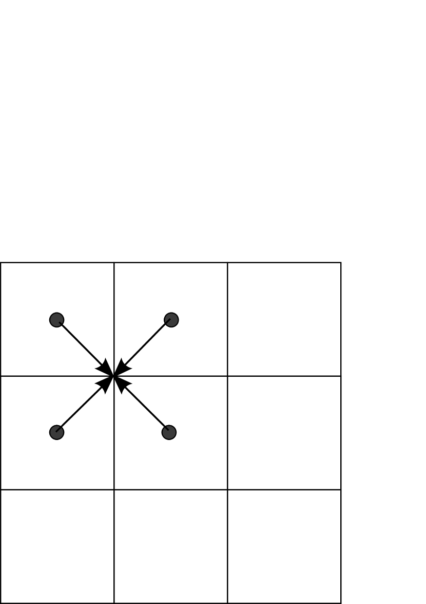
(a)

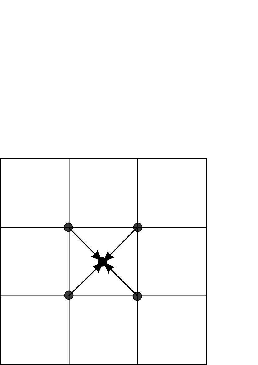
(b)

(c)

Figure 1: Scheme for calculating space-averaged velocities. Project of the normal velocities from the cell centers to the corner of cells (a), from the cells to the center (b) by means weight template (c).

where $\widetilde{v_{L}}$ and $\widetilde{v_{R}}$ are defined using a two-level scheme. At the first level, we project the normal velocities from the cell centers to the corner of the neighboring cells (see fig. 1a), thus taking into account the information from the cells in the direction perpendicular to the $x$-direction. At the second level, we project the normal velocities from the cell corners to the center of the given cell (see fig. 1b). This value will be used to define $\widetilde{v_{L}}$ and $\widetilde{v_{R}}$. The weight template is shown in Figure (1c). For convenience, we give an explicit formula to compute velocity $\widetilde{v}$ in cell $(i,k,l)$

$$\widetilde{v}_{(i,k,l)}=\frac{1}{16}\left(v_{i,k+1,l+1}+v_{i,k+1,l-1}+v_{i,k-1,l+1}+v_{i,k-1,l-1}\right)+$$ (45)

$$\frac{1}{8}\left(v_{i,k+1,l}+v_{i,k-1,l}+v_{i,k,l+1}+v_{i,k,l-1}\right)+\frac{1}{4}v_{i,k,l}.$$

This approach is based on the geometric transformation described in [11, 50], which takes into account fluxes from all possible directions. Of course, multidimensional Riemann solvers can also be used [31, 32, 33, 34, 35, 36, 37, 38, 39], which may be important when solving the multidimensional magnetohydrodynamics equations.

Now, we present the detailed algorithm for computing the Lagrangian step for hydrodynamic variables $f$ (density, momentum, internal and total energies) in each cell $(i,k,l)$ of the computational domain. Equation (39) in the Cartesian coordinates has the following form:

$$\frac{f^{n+1}_{i,k,l}-f^{n+1/2}_{i,k,l}}{\tau}=-\frac{F^{x}_{i+1/2,k,l}-F^{x}_{i-1/2,k,l}}{h_{x}}-\frac{F^{y}_{i,k+1/2,l}-F^{y}_{i,k-1/2,l}}{h_{y}}-\frac{F^{z}_{i,k,l+1/2}-F^{z}_{i,k,l-1/2}}{h_{z}}.$$

We consider the flux of $f$ along the $x$-direction ($i$-index), the other two fluxes can be computed by analogy. First, we calculate the values of $\widetilde{v}_{x}$ in cells $i-1$, $i$, and $i+1$ using the following equation:

$$\widetilde{v}_{x,([i\pm 1,i],k,l)}=\frac{1}{16}\left(v_{x,([i\pm 1,i],k+1,l+1)}+v_{x,([i\pm 1,i],k+1,l-1)}+v_{x,([i\pm 1,i],k-1,l+1)}+v_{x,([i\pm 1,i],k-1,l-1)}\right)+$$

$$\frac{1}{8}\left(v_{x,([i\pm 1,i],k+1,l)}+v_{x,([i\pm 1,i],k-1,l)}+v_{x,([i\pm 1,i],k,l+1)}+v_{x,([i\pm 1,i],k,l-1)}\right)+\frac{1}{4}v_{x,([i\pm 1,i],k,l)}.$$

Second, we compute $\widehat{v}_{x}$ using Equation (44):

$$\widehat{v}_{x,i+1/2,k,l}=\frac{\widetilde{v}_{x,(i+1,k,l)}\sqrt{\rho_{i+1,k,l}}+\widetilde{v}_{x,(i,k,l)}\sqrt{\rho_{i,k,l}}}{\sqrt{\rho_{i+1,k,l}}+\sqrt{\rho_{i,k,l}}},$$

$$\widehat{v}_{x,i-1/2,k,l}=\frac{\widetilde{v}_{x,(i-1,k,l)}\sqrt{\rho_{i-1,k,l}}+\widetilde{v}_{x,(i,k,l)}\sqrt{\rho_{i,k,l}}}{\sqrt{\rho_{i-1,k,l}}+\sqrt{\rho_{i,k,l}}}.$$

Finally, the fluxes of hydrodynamic variables can be computed based on Equation (41) as follows:

$$F^{x}_{i+1/2,k,l}=\widehat{v}_{x,i+1/2,k,l}\times\left\{\begin{array}[]{c}f_{i,k,l}(-|\widehat{v}_{x,i+1/2,k,l}|t),\widehat{v}_{x,i+1/2,k,l}\geq 0\\ f_{i+1,k,l}(|\widehat{v}_{x,i+1/2,k,l}|t),\widehat{v}_{x,i+1/2,k,l}<0\end{array}\right.,$$

$$F^{x}_{i-1/2,k,l}=\widehat{v}_{x,i-1/2,k,l}\times\left\{\begin{array}[]{c}f_{i-1,k,l}(-|\widehat{v}_{x,i-1/2,k,l}|t),\widehat{v}_{x,i-1/2,k,l}\geq 0\\ f_{i,k,l}(|\widehat{v}_{x,i-1/2,k,l}|t),\widehat{v}_{x,i-1/2,k,l}<0\end{array}\right..$$

We compare the 1-point stencil and 9-point stencil approaches for calculating the velocities $u_{\rm L}$ and $u_{\rm R}$ on the problem of rotating gaseous disk. For this test problem, we define the gas density and pressure as:

$$p(r)=\rho(r)=\left\{\begin{array}[]{c}2-r,r<1\\ 1,r\geq 1\end{array}\right.,$$

$$\omega(r)=\left\{\begin{array}[]{c}1,r<1\\ 0,r\geq 1\end{array}\right..$$

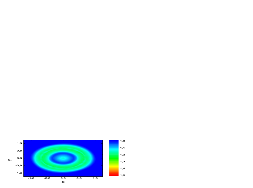
Figure 2: Rotation of a gaseous disk. Left: velocity is defined using Equation (42). Right: velocity is defined using Equation (44).

Figure (2) shows the results of using of the 1-point stencil (left) and 9-point stencil (right) for the definition of velocity at the Lagrangian step. The red points visible in the left panel are the geometrical artifacts and they disappear when applying the 9-point stencil.

2.4 The conservation of total energy

Our system of hydrodynamics equations is overdefined. We use two approaches to conserve the total energy:

1. Renormalization of the absolute value of the velocity, with each component of the velocity remaining unchanged (on boundary gas-vacuum) [13]:

   $$|\vec{v}|=\sqrt{2(E-\epsilon)}.$$

2. The internal energy (or entropy) correction [29]:

   $$|\rho\epsilon|=\left(\rho E-\frac{\rho\vec{v}^{2}}{2}\right).$$

In the very low density regions (more than five orders of magnitude lower than the mean density), we use the first approach, while in the other regions the second approach is applies. Such a modification of the method keeps the detailed energy balance and guaranteed non-decrease of entropy. Similar approaches were used in [40, 41]. Other authors using approach for retaining positivity of pressure and conservation [42, 43], which are particularly important at high Mach number.

2.5 The Poisson solver

Our hydrodynamics equations include the effect of self-gravity. It is therefore necessary to compute the gravitational potential using the gas current density distribution. In our method, we use a finite-difference representation of the Poisson equation on the 27-point stencil:

$$-\frac{38}{9}\Phi_{i,k,l}+$$ (46)

$$\frac{4}{9}\left(\Phi_{i-1,k,l}+\Phi_{i+1,k,l}+\Phi_{i,k-1,l}+\Phi_{i,k+1,l}+\Phi_{i,k,l-1}+\Phi_{i,k,l+1}\right)+$$

$$\frac{1}{9}\left(\Phi_{i-1,k-1,l}+\Phi_{i+1,k-1,l}+\Phi_{i-1,k+1,l}+\Phi_{i+1,k+1,l}+\Phi_{i-1,k,l-1}+\Phi_{i+1,k,l-1}\right.+$$

$$\left.\Phi_{i-1,k,l+1}+\Phi_{i+1,k,l+1}+\Phi_{i,k-1,l-1}+\Phi_{i,k+1,l-1}+\Phi_{i,k-1,l+1}+\Phi_{i,k+1,l+1}\right)+$$

$$\frac{1}{36}\left(\Phi_{i-1,k-1,l-1}+\Phi_{i-1,k+1,l-1}+\Phi_{i-1,k-1,l+1}+\Phi_{i-1,k+1,l+1}\right.+$$

$$\left.\Phi_{i+1,k-1,l-1}+\Phi_{i+1,k+1,l-1}+\Phi_{i+1,k-1,l+1}+\Phi_{i+1,k+1,l+1}\right)=4\pi Gh^{2}\rho_{i,k,l}.$$

The main motivation for the 27-point stencil is the Galilean invariance of the numerical solution. The algorithm for solving Equation 46 consists of the following several stages.

Stage 1. Formulation of boundary conditions for Poisson equation. To find the gravitational potential at the boundaries, we use the first two terms of the multipole expansion:

$$\Phi(x,y,z)|_{D}=-\frac{M}{r}-\frac{1}{r^{3}}\left(I_{x}+I_{y}+I_{z}-3I_{0}\right),$$ (47)

where

$$I_{0}=\frac{\left(x^{2}I_{x}+y^{2}I_{y}+z^{2}I_{z}\right)-2\left(xyI_{xy}+xzI_{xz}+yzI_{yz}\right)}{r^{2}},$$ (48)

$$I_{x}=\sum_{j}\left(z^{2}_{j}+y^{2}_{j}\right)m_{j}\qquad I_{y}=\sum_{j}\left(x^{2}_{j}+z^{2}_{j}\right)m_{j}\qquad I_{z}=\sum_{j}\left(x^{2}_{j}+y^{2}_{j}\right)m_{j},$$ (49)

$$I_{xy}=\sum_{j}x_{j}y_{j}m_{j}\qquad I_{xz}=\sum_{j}x_{j}z_{j}m_{j}\qquad I_{yz}=\sum_{j}y_{j}z_{j}m_{j},$$ (50)

where $x,y,z$ are the coordinates of the boundary cells, $r=\sqrt{x^{2}+y^{2}+z^{2}}$ the distance from the boundary cells to the coordinate center, $x_{j},y_{j},z_{j}$ the coordinates of computational cells, $m_{j}$ the mass in each cell, $M$ the total mass in the computational domain, and the summation is performed over all grid cells. Whenever boundary values of the potential appear on the left-hand side of Equation (46), they are taken to the right-hand side and added to the density term.

Stage 2. The Fourier transformation of density to the harmonic space. In the second step, we take a direct Fourier transform of the density to obtain their harmonic amplitudes

$$\sigma_{j,m,n}=\sum_{i,k,l}\rho_{i,k,l}exp\left(-\frac{\vec{i}2\pi ij}{I}-\frac{\vec{i}2\pi km}{K}-\frac{\vec{i}2\pi ln}{L}\right),$$ (51)

where $I,K,L$ is number of cells along coordinates, $\vec{i}$ is the imaginary unit.

Stage 3. The solution of Poisson equation in the harmonic space. We assume that the gravity is represented as a superposition of eigenfunctions of the Laplace operator:

$$\Phi_{i,k,l}=\sum_{j,m,n}\phi_{j,m,n}exp\left(\frac{\vec{i}2\pi ij}{I}+\frac{\vec{i}2\pi km}{K}+\frac{\vec{i}2\pi ln}{L}\right).$$ (52)

After substituting this expansion into equation (46), we obtain a simple formula to compute the harmonic amplitudes of the gravitational potential:

$$\phi_{j,m,n}=\frac{\frac{2}{3}\pi h^{2}\sigma_{j,m,n}}{1-\left(1-\frac{2sin^{2}\frac{\pi j}{I}}{3}\right)\left(1-\frac{2sin^{2}\frac{\pi m}{K}}{3}\right)\left(1-\frac{2sin^{2}\frac{\pi n}{L}}{3}\right)}.$$ (53)

To transform the gravitational potential from the harmonic space into the physical space, the inverse Fourier transform is used. For the numerical implementation of the Fast Fourier Transform, we use the FFTW library [44].

The verification of the Poisson equation solver was done on the following density profile

$$\rho(r)=\left\{\begin{array}[]{@{\,}r@{\quad}l@{}}2r^{3}-2r^{2}+1,&r\leq 1\\ 0,&r>1\end{array}\right.,$$

which has the following analytical solution

$$\Phi(r)=\left\{\begin{array}[]{@{\,}r@{\quad}l@{}}\frac{4\pi}{15}r^{5}-\frac{3\pi}{5}r^{4}+\frac{2\pi}{3}r^{2}-\frac{3\pi}{5},&r\leq 1\\ -\frac{4\pi}{15r},&r>1\end{array}\right..$$

Table (1) shows the behavior of the numerical solution on a sequence of meshes with increasing numerical resolution. Our method is fourth-order accurate.

3 DISCUSSION

The limiter problem. The main trend in constructing accurate numerical methods (e.g. PPM, TVD and WENO) has been the use of high-order polynomials in the interpolation schemes. However, this practice often produces unphysical oscillations around discontinuous solutions. To resolve this problem, the limiters are introduced to create a monotonic interpolation scheme and remove nonphysical extrema [45, 46, 47]. However, the use of different limiters results often in the incorrect calculation of the shock wave velocity. The operator splitting approach allows us to use limiters only when calculating piecewise parabolic functions in, e.g., equations (33), (34), and (41). We do not provide a rigorous proof here, but we simply state that this property of our scheme has been experimentally confirmed.

The Roe average. In our numerical scheme, we provide a modification of the classic Roe space-averaging of hydrodynamic variables, which behaves better on modelling the gas-vacuum boundary. In fact, the use of the classic Roe scheme for density at the gas-vacuum boundary (and, in general, at any high density and pressure jumps) yields too large sound speeds. In general, the gas-vacuum boundary should be modelled by means a gas kinetic approach because of low collision frequency between gas particles, but that it is technically not feasible today.

Advantages and disadvantages of our numerical method. In our understanding, the advantages of our numerical scheme are: 1) accuracy on sufficiently smooth solutions and low dissipation on discontinuous solutions, 2) limiter-free and artificial-viscosity-free implementation, 3) Galilean invariance, 4) guaranteed non-decrease of the entropy [29], 5) extensibility on other hyperbolic models, 6) simplicity of program implementation, and 7) high scalability. We note that the use of a computational mesh results in distortion of the numerical solution. In the case of complex nonlinear hydrodynamic flows, such distortions can lead to the artificial alignment of the numerical solution with the cell boundaries. The use of non-regular or adaptive meshes alleviates but does not resolve this problem. Therefore, it is desirable to construct Galilean invariant numerical schemes, which produce numerical solutions that does not depend on the orientation of the computational mesh. We think that our numerical method can be effectively implemented on GPUs, as the GPUPEGAS code [48], and on the Intel Phi architecture, as the AstroPhi code [49], because it uses the same algorithms.

Our numerical method has disadvantages, the three most significant of which we discuss below:

1. A rather simple finite-difference scheme for the time derivative. By example, the WENO code uses the Runge-Kutta fourth-order-accurate scheme for the time derivative. The advantage of such multilayer schemes is the expansion of the computational stencil (on regular 3D mesh to $9^{3}$ cells). It is a very strong solution for the Galilean invariance problem.

2. The construction of the interpolation parabola for problems with complex geometries. When using non-regular meshes (e.g. triangle cells), the construction of piecewise parabola is a non-trivial problem, which requires the use of a special spline technique adapted to cells with an arbitrary simplex of cells.

3. At the Eulerian step we solve the Riemann problem, which in turn relies on the analytic solution of the spectral problem (because the numerical solution of the eigenvalue/eigenvector problem is ill-posed). Finding the analytic solution for any hyperbolic equations is difficult. A possible solution is to use ”the potentials technique” [50], but this technique requires the singular value decomposition of matrices, which is very expensive.

The future work. In the future, we plan to expand our numerical method to ”collisionless” hydrodynamics, which solves for the first three moments of the collisionless Boltzmann equation [7, 51]. The main features of this expansion will be the formulation of the equation of state for collisionless component and the development of thermodynamically consistent star formation process with guaranteed non-decrease of the entropy.

4 THE VERIFICATION OF NUMERICAL METHOD

In this section, we test the performance of our numerical code using a comprehensive set of test problems. For all numerical simulations, a CFL number equal to 0.2 was used.

4.1 The Sod shock-tube problem

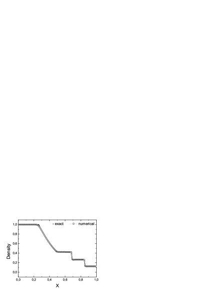
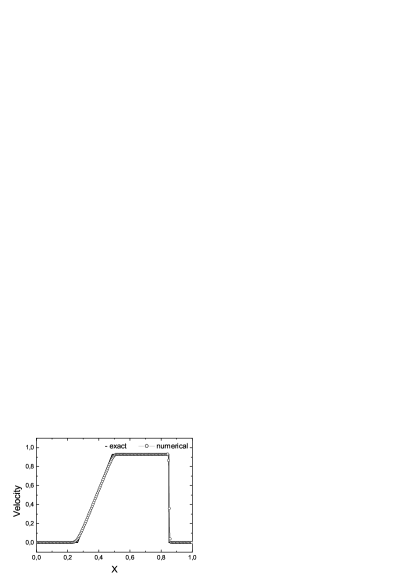
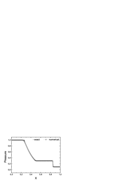
Figure 3: Results of the first shock tube problem.

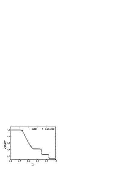
Figure 6: Comparison of the first-order (left) and higher-order (right) methods using the first Sod shock tube problem.

We choose the shock-tube problem to demonstrate the advantages of using our high-order method for simulating discontinuities with low dissipation. This test can also highlight problems with simulating the rarefaction waves, since many methods are known to produce a non-physical increase of the internal energy in the rarefaction region. Moreover, a large initial drop of pressure (five orders of magnitude) is the standard robustness test showing the capability of numerical methods to simulate the strong perturbations with quickly spreading shock waves. The initial configurations for three different tests are shown in Table (2), where $x_{0}$ is the position of the interface between two initial states and indexes L and R represent the l.h.s. and r.h.s. states, respectively. For this test, we use hundred grid cells. The results of simulations are shown in Figures (3), (4), and (5), and the comparison of the high-order and first-order methods is presented in Figure (6).

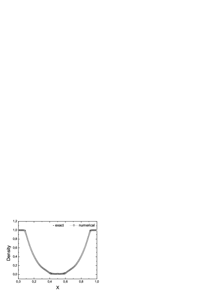
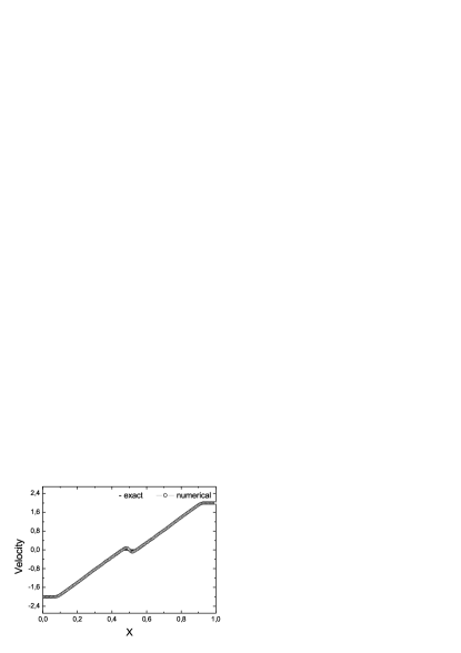
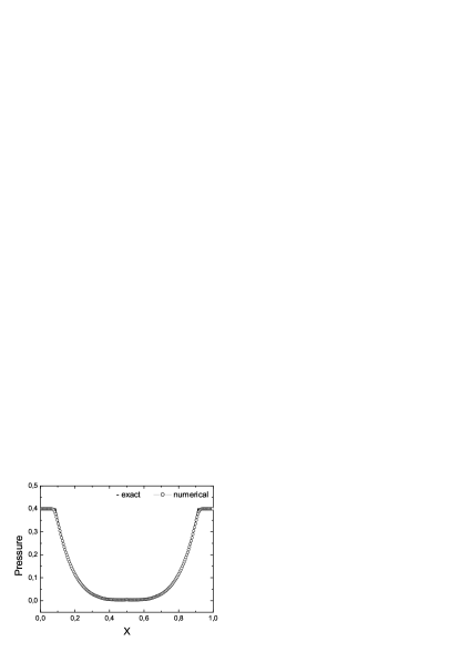
Figure 4: Results of the second shock tube problem.

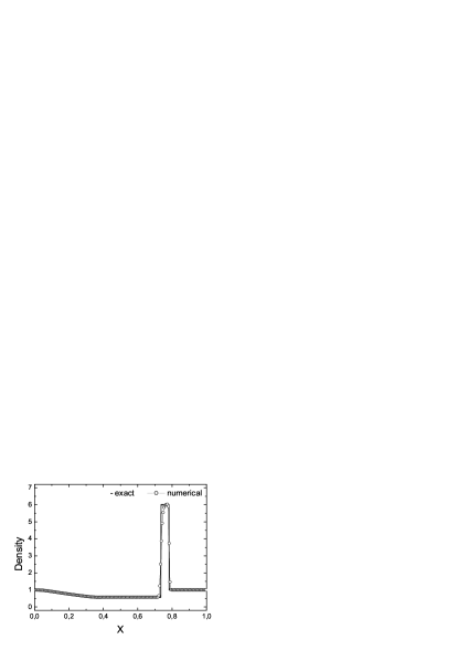
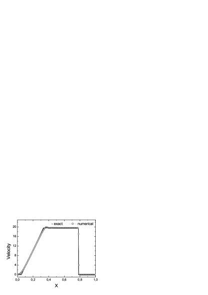
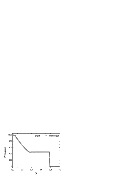
Figure 5: Results of the third shock tube problem.

The main purpose of the first test shown in Figure (3) is the correct simulation of the shock wave region. Our numerical method performs well on this problem, showing low dissipation and no unphysical oscillations. When compared with the first-order method, the number of cells over which the shock is spread reduces from 12 to just two (see Figure 6). The main purpose of the second test shown in Figure (4) is to test the code’s ability to simulate correctly the rarefaction region. The main purpose of the third test shown in Figure (5) is to test the code’s ability to simulate correctly the strong shock wave. Our numerical method correctly reproduces all types of solutions.

4.2 Simulation of the Kelvin-Helmholtz and Releigh-Taylor instabilities.

It is important to show that our numerical method does not suppress physical instabilities that may develop during numerical simulations. To check this, we investigated the growth of the Rayleigh-Taylor and Kelvin-Helmholtz instabilities. The Rayleigh-Taylor instability arises at the interface of two fluids with different densities when the lighter fluid pushes against the heavier one due to gravitational acceleration and the Kelvin-Helmholtz instability arises at the interface of two fluids moving with respect to each other. Both instabilities give rise to nonlinear hydrodynamic turbulence.

To simulate the development of the Kelvin-Helmholtz instability, we set up a square region with size of $[-0.5:0.5]^{2}$. The initial density and the x-component of velocity are chosen as:

$$\rho_{0}(x,y)=\left\{\begin{array}[]{c}1,|y|>0.25+0.01(1+cos(8\pi x))\\ 2,|y|\leq 0.25+0.01(1+cos(8\pi x))\end{array}\right.,$$

$$v_{x,0}(x,y)=\left\{\begin{array}[]{c}-0.5,|y|>0.25+0.01(1+cos(8\pi x))\\ 0.5,|y|\leq 0.25+0.01(1+cos(8\pi x))\end{array}\right..$$

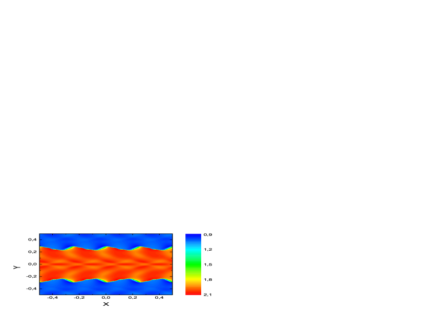
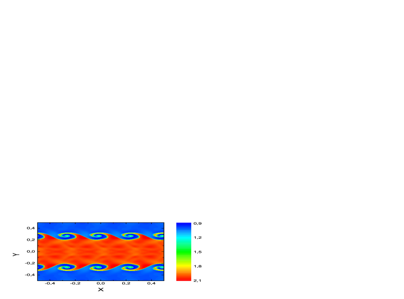
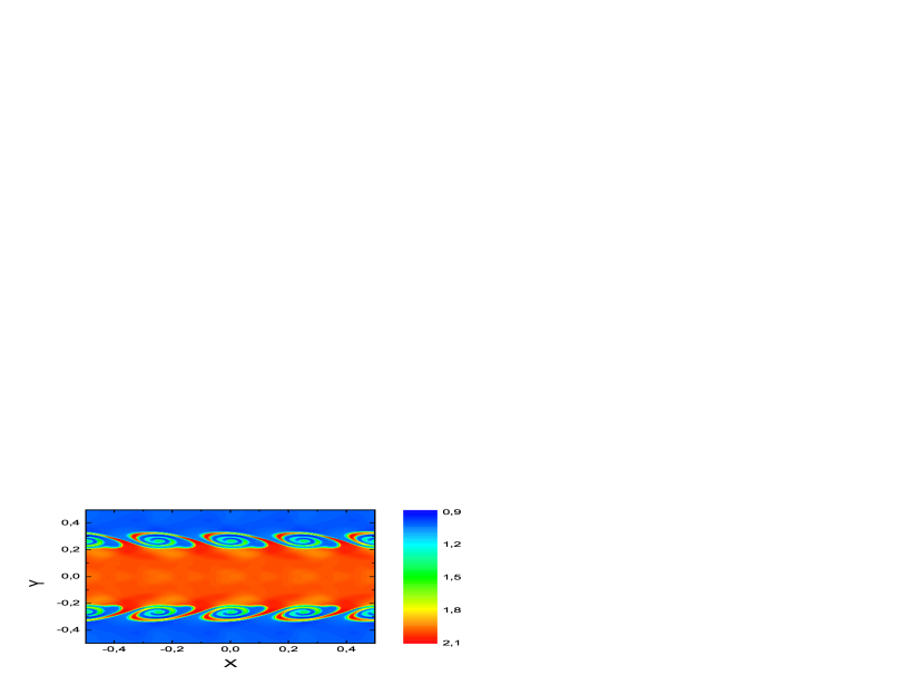
Figure 7: Development of the Kelvin-Helmholtz instability. The evolution times are 0.0 (top-left), 0.2 (top-right), 0.5 (bottom-left) and 0.8 (bottom-right).

Here, the perturbation to the interface between two fluids is set by a cosine wave with amplitude $A=0.01$ and wave number $k=4$. The gas pressure is set to $p=2.5$ and the adiabatic index is set to $\gamma=1.4$. A small sinusoidal perturbation is given to both the gas density and velocity in order to initiate the growth of the instability. For numerical simulations, a computational mesh of $256^{2}$ grid zones was used. The development of the Kelvin-Helmholtz instability is shown in Figure (7). To calculate the characteristic growth time of the Kelvin-Helmholtz instability we use the following formula:

$$\tau_{KH}=\frac{\lambda\left(\rho_{in}+\rho_{out}\right)}{v_{rel}\sqrt{\rho_{in}\rho_{out}}},$$ (54)

where $\lambda=1/4$ is the inverse frequency of the sinusoidal perturbation, $v_{rel}=1$ the relativity velocity between both fluids, $\rho_{in}=2$ the density in the inner region, and $\rho_{out}=1$ the density in the outer region. For these parameters, $\tau_{KH}\approx 0.53$, which is in good agreement with our test simulations shown in Figure (7). Indeed, fully developed turbulent eddies at the interface between two fluids occur at $t>0.5$.

To simulate the Rayleigh-Taylor instability, we set the $[-0.25;0.25]\times[-1.5;1.5]$ box with the following parameters:

$$\rho_{0}(x,y)=\left\{\begin{array}[]{c}1,|y|>0.75\\ 2,|y|\leq 0.75\end{array}\right.,$$

$$p=0.15-\rho\cdot g\cdot|y|,$$

where $p$ is the pressure in hydrostatic equilibrium, $g=0.1$ the acceleration of free fall, $y$ the vertical coordinate, and $\gamma=1.4$.

The initial hydrostatic equilibrium receives a perturbation of the form: $v_{y,0}(x,y)=A(|y|-0.75)[1+cos(2\pi x)][1+cos(2\pi y)]$, where

$$A(y)=\left\{\begin{array}[]{c}10^{-2},|y|\leq 0.01\\ 0,|y|>0.01\end{array}\right..$$

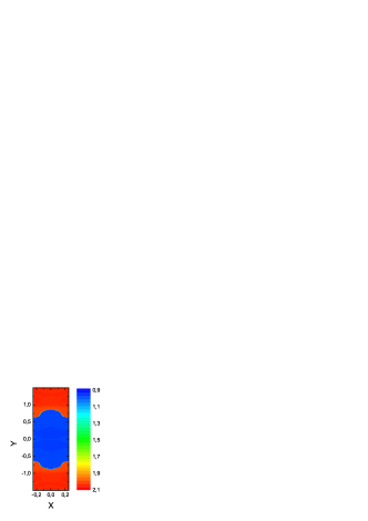
Figure 8: Development of the Rayleigh-Taylor instability. The evolution times are 0.0 (top-left), 7.0 (top-right), 10.0 (bottom-left), and 13.0 (bottom-right).

For numerical simulations, a computational mesh of $100\times 600$ grid zones was used. The development of the Rayleigh-Taylor instability is shown in Figure (8). To analyse the growth of the Rayleigh-Taylor instability, we use the following formula for the perturbation amplitude

$$p(t)=0.01exp\left(t\sqrt{Ag}\right)\simeq 0.01exp\left(0.25t\right),$$ (55)

where $A=2/3$ is the Atwood number. For example, at $t=13$ the perturbation amplitude is $p(t=13)\simeq 0.25$, which is in good agreement with our simulations. Indeed, the initial location of the interface between two fluids is at $y=\pm 0.75$. By the time $t=13$, the density perturbation has propagated by approximately $dy=\pm 0.25-0.3$.

4.3 The Sedov blast wave

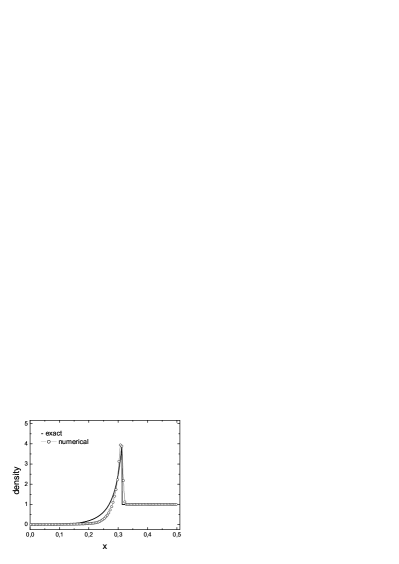
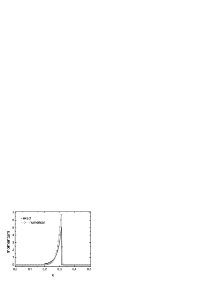
Figure 9: Density (left) and momentum (right) in the Sedov blast wave problem. The solid lines represent the exact solution.

The Sedov blast is a spherical explosion caused by the point injection of energy and in astronomy is representative of a supernova explosion. The initial setup for this test is as follows: $[-0.5;0.5]^{3}$ is the computational domain, $\gamma=5/3$ the adiabatic index, $\rho_{0}=1$ the initial density, and $p_{0}=10^{-5}$ the initial pressure. At time $t=0$, the thermal energy $E_{0}=0.6$ is injected. The energy is injected in a central sphere with radius $r_{central}=0.02$. For numerical simulations, a computational mesh of $100^{3}$ grid zones was used. The resulting radial profiles of the density and momentum at time $t=0.05$ are shown in Figure (9).

The Sedov blast wave problem is the standard test which verifies the code’s ability to manage strong shocks with high Mach numbers. The sound speed of the background medium is negligibly small, so that the Mach number is high $M=1432$. Our numerical method performs at this difficult problem quite well and reproduces accurately the position of the shock and profile of the shock wave in the wake.

4.4 The expansion of gas into vacuum

Numerical hydrodynamics methods that use the classic Roe space-averaging scheme for gas density behave poorly on the gas-vacuum boundary. Thanks to the special space-averaging scheme (see Section 1.1), our numerical method can model the gas-vacuum boundary with conservation of total energy. To demonstrate this, we set up a test problem describing the expansion of gas into vacuum. More specifically, we set up a gas sphere with unit radius on the $[-2;2]^{3}$ domain:

$$p_{0}(r)=\rho_{0}(r)=\left\{\begin{array}[]{c}1,r\leq 1\\ 0,r>1\end{array}\right..$$

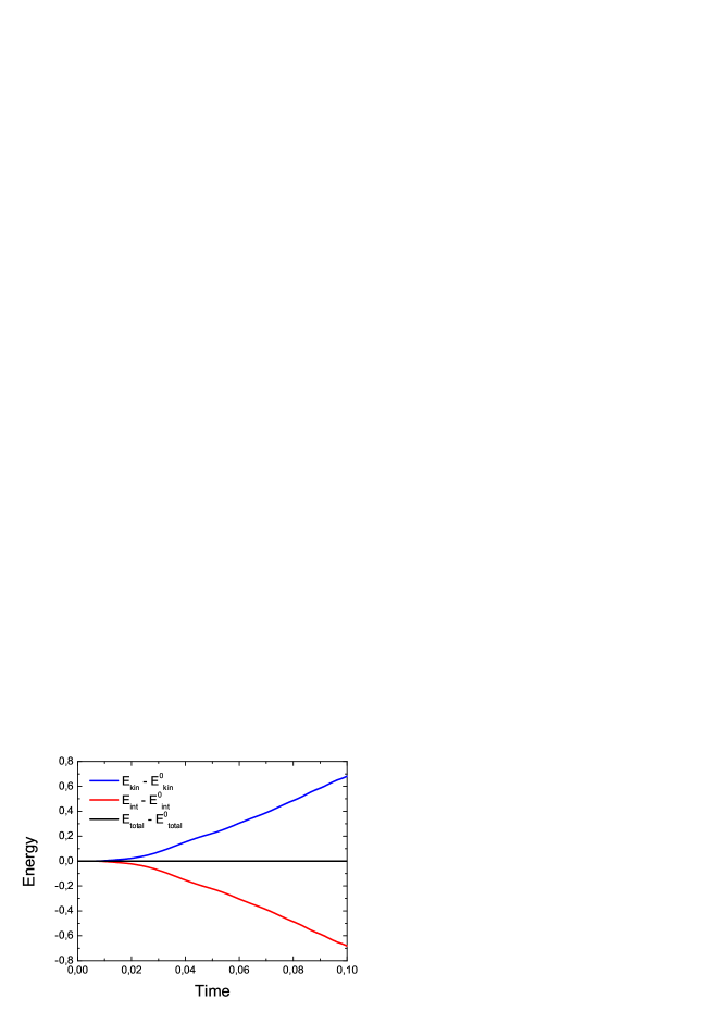
Figure 10: Time evolution of the kinetic, internal, and total energies with respect to their initial values in the test problem with expansion of gas into vacuum.

The ratio of specific heats $\gamma=1.4$ and initial velocity $\vec{v}$ is set to zero. For numerical simulations, a computational mesh of $256^{3}$ grid zones was used. The behaviour of the kinetic, internal, and total energies of gas are shown in Figures (10). As expected, the kinetic energy increases owing to expansion of gas into vacuum, the internal energy decreases owing to adiabatic cooling, but the total energy stays constant within the machine precision.

It’s the synthetic test for control of total energy behaviour for the expand of gas cloud to vacuum. On realistic astrophysical simulations don’t use a vacuum region, but numerical method must be able to simulate such regions with conservation of total energy.

4.5 Three test problem of Calella & Woodward (1984)

To further verify our numerical hydrodynamics scheme, three test problem from [52] were used: two interacting blast waves, a Mach 3 wind tunnel with a step, and double Mach reflection of a strong shock. We note that these test problems do not have analytic solutions or predictions, unlike other tests used in our paper.

4.5.1 Two Interacting Blast Waves

This test is designed to check the code’s ability to simulate the interaction of strong shock waves in a narrow region. The initial density is set to unity and the velocity is zero everywhere on the $[0;1]$ domain. The pressure for $x<0.1$ is set to $p_{L}=1000$, while for $0.1<x<0.9$ and $x>0.9$it is set to $p_{C}=0.01$ and $p_{R}=100$, respectively. Reflecting boundary conditions are used. For numerical simulations, a computational mesh of $2400$ grid zones was used. The result of numerical simulation is presented in Figure (11). Our numerical scheme correctly reproduces the position of shock waves and contact discontinuities, but similar to many other numerical schemes smears somewhat the contact discontinuity at $x=0.6$. The shock wave at $x=0.76$ has a correct amplitude of $\approx 6.5$ and the precursor wave at $x=0.86$ has a correct amplitude of $\approx 1.0$. The velocity field having two peak at $x=0.65$ and $x=0.86$ is also correctly reproduced in our test problem. We note that we used an equidistant mesh, while Woodward & Colella used adaptive meshes.

4.5.2 A Mach 3 Wind Tunnel with a Step

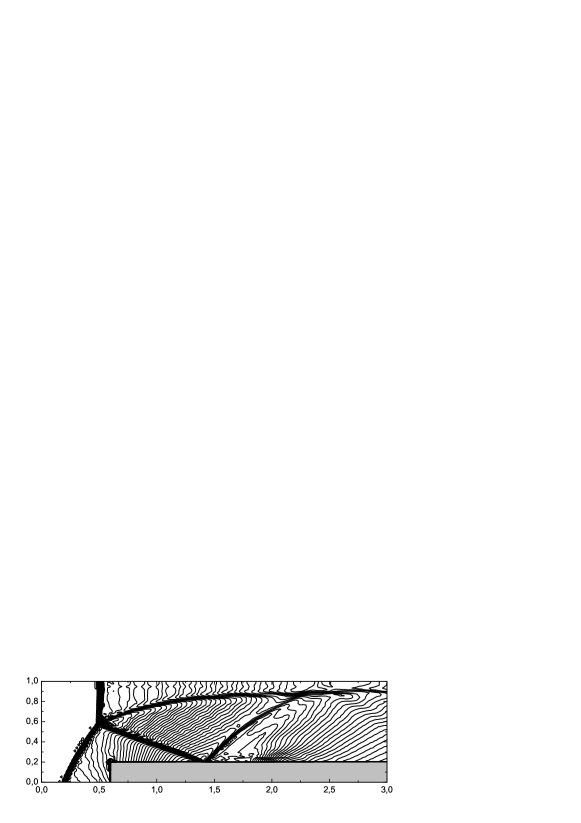
Figure 12: The a Mach 3 wind tunnel with a step problem. The isolines of density for computational mesh of $720\times 240$ (bottom) grid zones

In this test problem, a flow with a Mach number equal to 3 is set in a tunnel with dimensions $[0;3]\times[0;1]$ containing a step. More specifically, the initial density and pressure are set to $\rho_{0}=1.4$ and $p_{0}=1$, respectively, the $y$-component of velocity is equal to zero, and the $x$-component of velocity is equal to 3.0 at $x<0.5$ and is zero elsewhere. The ratio of specific heats is $\gamma=1.4$. The inflow and outflow boundary conditions are chosen on the left and right boundaries, respectively, while on the top and bottom walls the reflecting boundary conditions are used. For numerical simulations, a computational mesh of $720\times 240$ grid zones was used. The results are presented in Figure (12). Evidently, our numerical scheme performs well on this difficult test problem. The position of all shock waves is correctly reproduced [53]. We note that in our method, we did not use any special adjustments for computing the singularity point at the corner of the step, in contrast to other numerical schemes [52]. This is due to a fundamental difference between the PPM and PPML methods, the latter using the local stencil for calculating the interpolation parabolas.

4.5.3 Double Mach Reflection of a Strong Shock

In this test problem, the reflection of a Mach 10 shock from an inclined plane is simulated. The initial density, pressure and velocity are set in the $[0;3.5]\times[0;1]$ domain as follows:

$$\rho_{0}=\left\{\begin{array}[]{c}8,x<1/2+y/tan(\pi/3)\\ 1.4,x\geq 1/2+y/tan(\pi/3)\end{array}\right.\qquad p_{0}=\left\{\begin{array}[]{c}116.5,x<1/2+y/tan(\pi/3)\\ 1,x\geq 1/2+y/tan(\pi/3)\end{array}\right.$$

$$v_{x,0}=\left\{\begin{array}[]{c}7.1447,x<1/2+y/tan(\pi/3)\\ 0,x\geq 1/2+y/tan(\pi/3)\end{array}\right.\qquad v_{y,0}=\left\{\begin{array}[]{c}-4.125,x<1/2+y/tan(\pi/3)\\ 0,x\geq 1/2+y/tan(\pi/3)\end{array}\right.,$$

the ratio of specific heats $\gamma=1.4$. On the left wall, the inflow boundary condition is set. On the right wall, on the top wall and on the bottom wall for $x<0.5$, the outflow boundary condition is used, while at the bottom wall for $x>0.5$ the reflection boundary condition is set. For numerical simulations, a computational mesh of $840\times 240$ grid zones was used. The results are presented in Figure (13). Our scheme performs well on this test problem. The position of all shock waves and contact discontinuities is reproduced correctly, similar to the classic PPM method of Woodward & Colella (1984). All shock waves are narrow, implying low dissipation, and exhibit no numerical artifacts near the boundaries. The reflected wave emerges from the bottom wall at $x=0.5$ and its amplitude reaches $\sim 0.5$ at $x=1.8$. At $x=2.6$ and $x=3.0$, the first and second triple Mach reflections are correctly reproduced.

4.6 The Aksenov Test

For the accuracy analysis of our numerical method we have chosen the Aksenov test [54]. It is a one-dimensional hydrodynamical test with the analytical periodic solution, which belongs to a class of infinitely differentiable functions. Let us consider the initial setup consisting of a density distribution of the following form

$$\rho=1+0.5\cos(x)$$ (56)

on the $x=[0:2\pi]$ domain with the periodic boundary conditions. The velocity is set to $u=0$ everywhere and the equation of state has the following form $p=\rho^{\gamma}$, where $\gamma=3$. Then the analytical solution is described as follows:

$$\rho=1+0.5\cos(x-ut)\cos(\rho t),$$ (57)

$$u=0.5\sin(x-ut)\sin(\rho t).$$ (58)

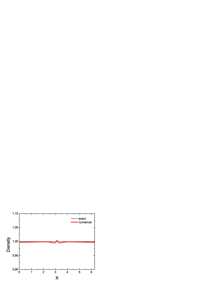
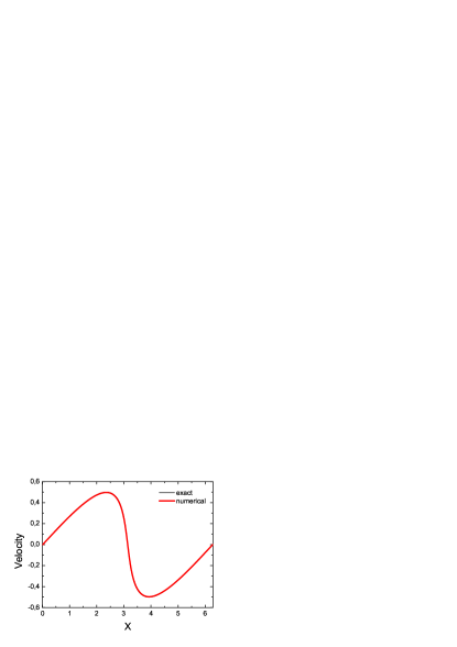
Figure 14: Results of the Aksenov test.

The results of the simulation for time $t=\pi/2$ are given in Figure (14). For the analysis of accuracy of our numerical method we use the following equation:

$$T=\log_{2}\left(\frac{E_{N}}{E_{N/2}}\right),$$ (59)

where $E_{N}=\sum_{1}^{N}|f_{i}^{\rm exact}-f_{i}^{\rm num}|$, $f_{i}^{\rm exact}$ is the exact solution of Aksenov test in cell $i$, $f_{i}^{\rm num}$ the numerical solution in cell $i$, and $N$ the number of grid zones. For this test problem, a computational mesh of $N=628$ grid zones was used. The resulting accuracy of our numerical scheme using the density distribution for $f_{i}$ is $T=1.713$.

5 NUMERICAL SIMULATION OF THE SPIRAL INSTABILITY IN A GALACTIC DISK

In this section, we will demonstrate the development of the spiral instability in a galactic disk adopting the isothermal approximation with $\gamma=1$. A thin gaseous disk is unstable to an axisymmetric perturbation if the Toomre $Q$-parameter is less than unity [55]:

$$Q=\frac{c_{s}\kappa}{\pi G\Sigma}<Q_{\rm crit}=1.0,$$ (60)

where $c_{s}$ is the sound speed, $\Sigma$ is the column density and $\kappa$ is the epicyclic frequency defined as:

$$\kappa^{2}=\frac{2\Omega}{r}\frac{d}{dr}\left(r^{2}\Omega\right)$$ (61)

where $\Omega$ is the angular velocity and $r$ is the radial coordinate. For local non-axisymmetric perturbations and three-dimensional disks with finite thickness, the critical Toomre parameter for the development of spiral instability can be somewhat greater, $Q_{\rm crit}\approx 1.5$ [56, 57].

The initial setup consists of a self-gravitating galactic gaseous disk submerged in a fixed dark matter (DM) halo of the following form:

$$\rho_{DM}=\frac{\rho_{0}}{1+\left(r/r_{0}\right)^{2}}$$ (62)

where $\rho_{0}=1.97M_{\odot}$ pc^-3 is the central DM density, $r_{0}=1.6$ kpc the characteristic scale length of the DM halo and $r_{h}=78.55$ kpc the halo radius. The DM mass is set to $5\times 10^{10}\leavevmode\nobreak\ M_{\odot}$. The details of the procedure for generating an equilibrium profile of a galactic gaseous disk in the gravitational potential of the DM halo can be found in [58].

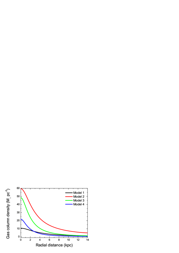
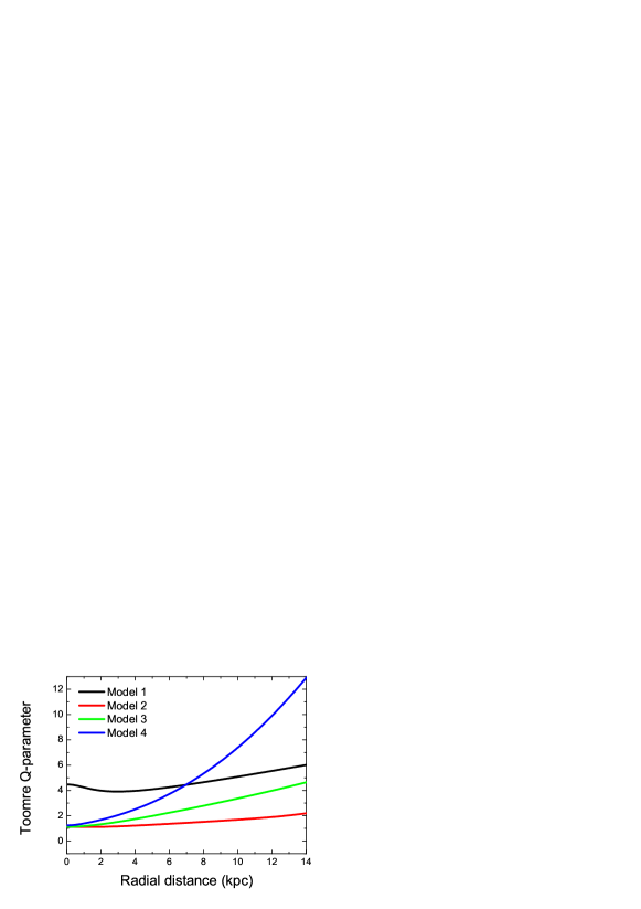
Figure 15: Initial profiles of column density (left) and Toomre $Q$-parameter (right) for all models.

We have considered four models, the parameters of which are listed in Table (3). The initial distributions of the gas column density $\Sigma$ and Toomre $Q-$parameter are shown in Figure (15). The gas temperature in models 1-3 is set to $T=10^{4}$ K, while in model 4 it equals to $T=2\times 10^{3}$ K. At the beginning of simulations, we introduce a small density perturbation characterized by a normal distribution with a zero mean and $10^{-4}$ root-mean-square deviation. For all numerical simulations a CFL number equal 0.2 and a computational mesh of $512^{3}$ grid zones are used.

To quantify the strength of spirals modes in numerical simulations of gravitationally unstable disks, we calculate the global Fourier amplitudes on the local sub-domain $r\leq R_{f}=8$ kpc, where $r$ is the distance from the coordinate center. The total computational box has the size of $[-16;16]^{3}$ kpc³:

$$A_{m}(t)=\frac{\left|\int\limits_{-R_{f}}^{R_{f}}\int\limits_{-\sqrt{R_{f}^{2}-x^{2}}}^{\sqrt{R_{f}^{2}-x^{2}}}\Sigma(x,y,t)e^{im\phi}dxdy\right|}{\int\limits_{-R_{f}}^{R_{f}}\int\limits_{-\sqrt{R_{f}^{2}-x^{2}}}^{\sqrt{R_{f}^{2}-x^{2}}}\Sigma(x,y,t)dxdy}$$ (63)

where $m=1,2,\ldots$ is the spiral mode, $\Sigma(x,y,y)$ the gas column density, and $\phi=\tan^{-1}(y/x)$ the polar angle. When the disk is axisymmetric, the amplitudes of all modes are equal to zero. When, say, $A_{m}(t)=0.1$, the amplitude of spiral modes is 10% that of the underlying axisymmetric density distribution.

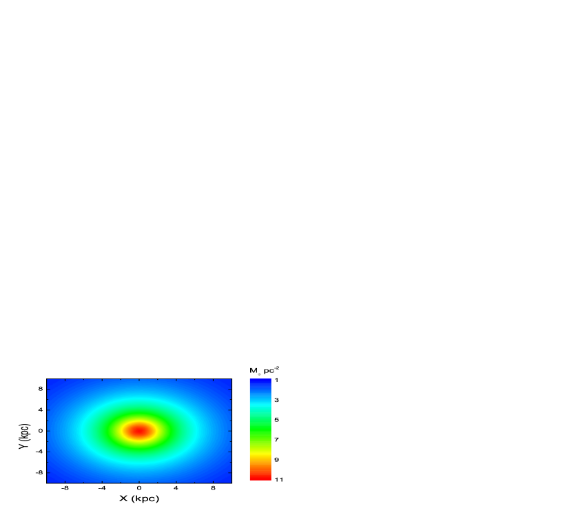
Figure 16: Evolution of the column density (in $M_{\odot}pc^{-2}$) in model 1. The evolution times are 0 Myr (top-left), 200 Myr (top-right), 300 Myr (bottom-left) and 400 Myr (bottom-right). The model is gravitationally stable.

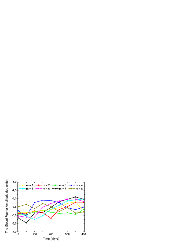
Figure 17: Time evolution of the global Fourier amplitudes (in log scale) in model 1.

Figure (16) shows the time evolution of the gas column density in model 1 during 400 Myr. The $Q$-parameter in this model is everywhere greater than a critical value of $Q_{\rm crit}\approx 1.5$. As expected, the initial perturbations die out with time and this model does not show any significant deviations from the initial near-axisymmetric state. The time behaviour of the global Fourier amplitudes shown in Figure (17) confirms our findings. The amplitudes of the first eight modes stay in the $(-6.0:-5.0)$ range (in the log scale), which corresponds to a 0.001% density perturbation relative to the underlying axisymmetric disk. The higher-order amplitudes show a similar behaviour. This test therefore confirms the expected stability of model 1 against small perturbations.

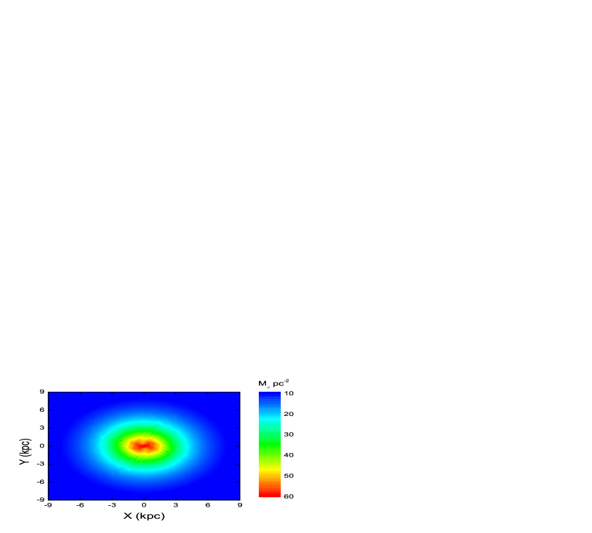
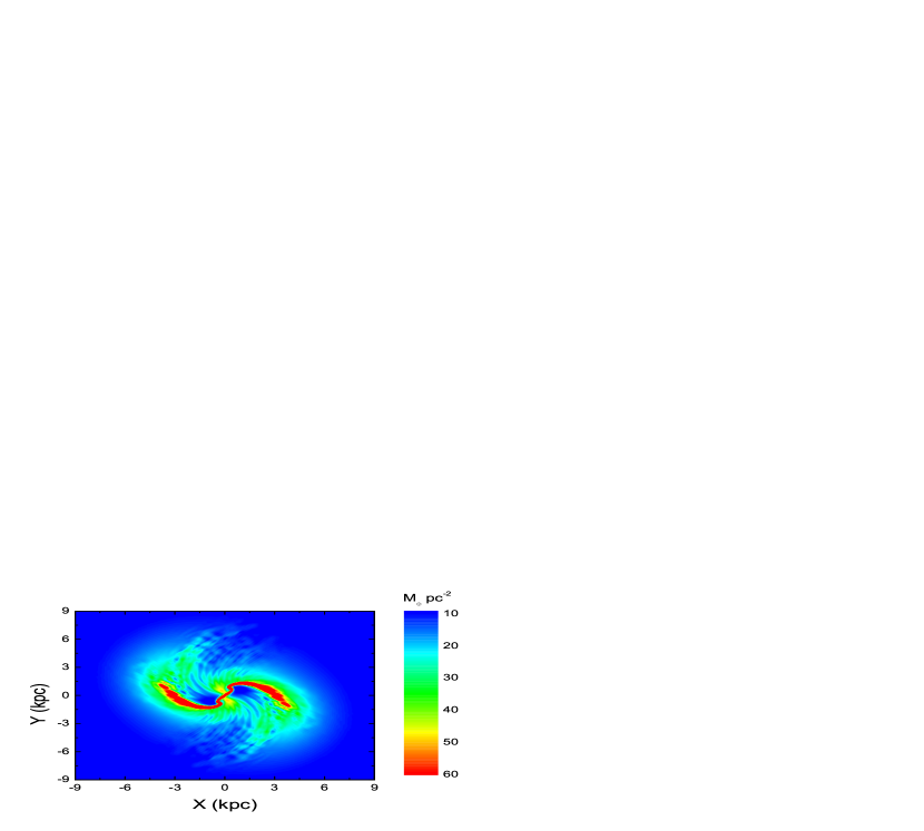
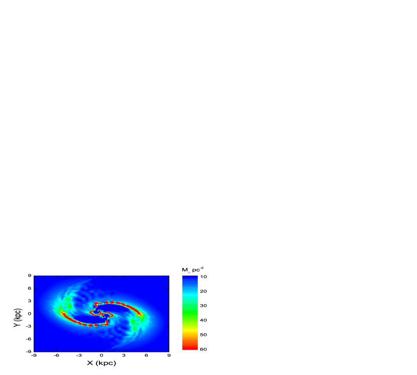
Figure 18: Evolution of the column density (in $M_{\odot}pc^{-2}$) in model 2. The evolution times are 0 Myr (top-left), 100 Myr (top-right), 200 Myr (bottom-left) and 280 Myr (bottom-right). The model is gravitationally unstable and develops a two-armed spiral pattern.

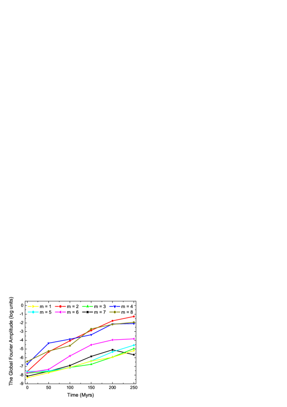
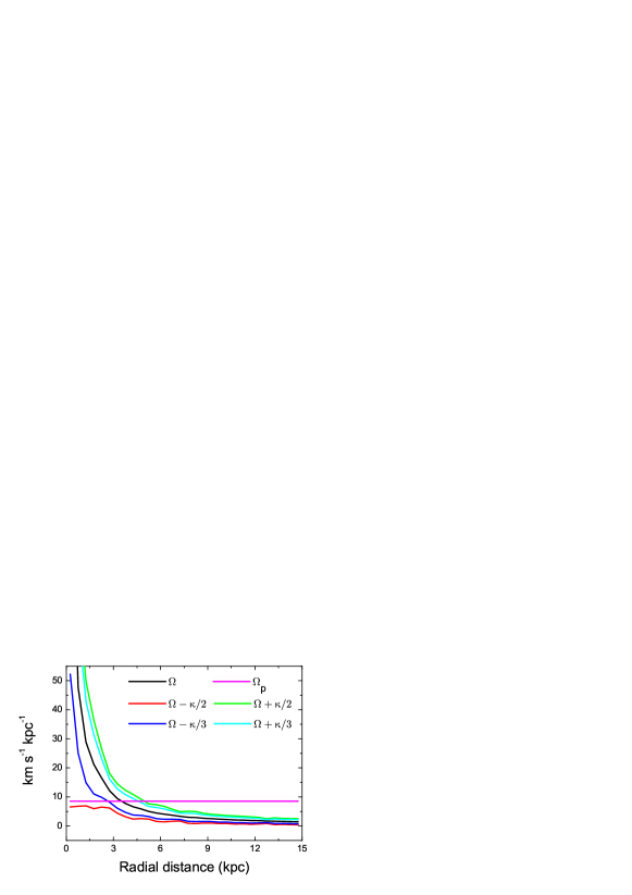
Figure 19: Top: Time evolution of the global Fourier amplitudes in model 2. Bottom: radial profiles of $\Omega$, $\Omega_{p}$, $\Omega\pm\kappa/2$, and $\Omega\pm\kappa/3$. The intersection of $\Omega_{p}$ with other profiles gives the position of resonances. In particular, the intersection of $\Omega_{p}$ with $\Omega-\kappa/3$ marks the position of the inner Lindblad resonance for the $m=3$ mode.

The time evolution of the gas column density in model 2 is presented in Figure (18). This model is characterized by the maximum disk mass and the highest ratio of the disk to DM halo mass, $\xi=0.1708$. The Toomre $Q$-parameter is the lowest among all four models and stays below a critical value of 1.5 in the inner 7 kpc. As a consequence, model 2 is very unstable and shows the development of a two-armed spiral pattern. The time evolution of the Fourier amplitudes in the upper panel of Figure (19) confirms our conclusions, demonstrating that the $m=2$, 4 and 8 modes are the fastest growing ones. By the end of simulations, the $m=2$ mode dominates and exceeds -1.5 in log units.

Why does our model disk develop a two-armed global spiral pattern rather than a three-armed or any other multi-armed pattern? The reason for the development of the $m=2$ mode can be understood when applying the swing amplification theory [59, 60, 61] The initial density perturbation applied to our model galactic disk creates a spectrum of disturbances. Amplification in a gravitationally unstable disk occurs when any leading spiral disturbance unwinds into a trailing one due to differential rotation. However, feedback loops that turn trailing disturbances into leading ones must be present in galactic discs in order for swing amplification to operate continuously [62]. Reflection of trailing spiral disturbances from a steep, high-$Q$ barrier [59] or propagation of trailing spiral disturbances through the galactic center naturally lead to the emergence of leading spiral disturbances and present positive feedback loops.

Regions with steeply increasing $Q$-parameters are absent in our model disc (see Fig. 15). Therefore, the propagation of disturbances through the disk centre presents the only possible feedback loop. This mechanism operates if there is no inner Lindblad resonance (ILR) for a specific spiral mode. The position of Lindblad resonances can be defined as

$$m(\Omega_{\rm p}-\Omega)=\pm\kappa,$$ (64)

where $\Omega_{\rm p}$ is the speed of the spiral pattern.

In the bottom panel of Figure (19) we plot the radial profiles of $\Omega_{\rm p}$, $\Omega\pm\kappa/m$, and $\Omega$ for the $m=2$ and $m=3$ modes. The intersection of $\Omega_{\rm p}$ with $\Omega-\kappa/2$ and $\Omega-\kappa/3$ gives the radial position of the ILRs for the $m=2$ and $m=3$ modes, respectively. Evidently, the ILR for the $m=2$ mode is absent, while it s present for the $m=3$ mode. Therefore, the $m=2$ trailing disturbances can propagate through the centre and emerge on the other side as leading ones, thus providing a feedback for the swing amplifier. As a result, the $m=2$ mode grows while the $m=3$ (and higher-$m$ modes) die out with time.

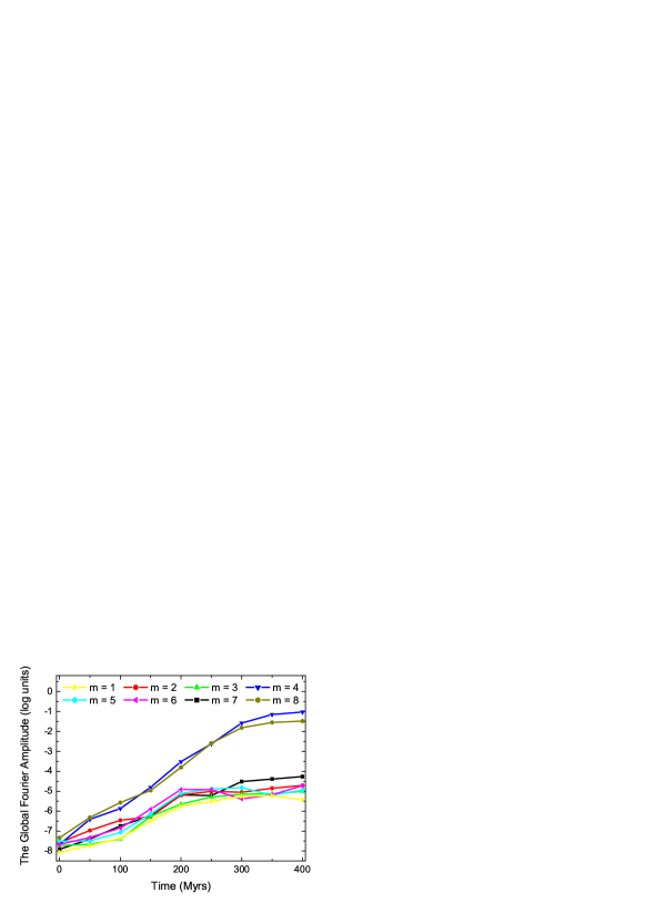
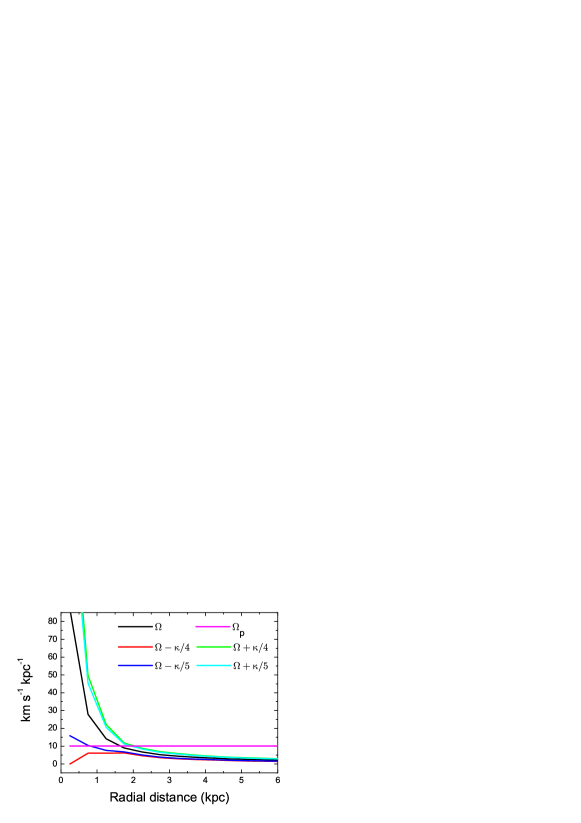
Figure 21: Top: Time evolution of the global Fourier amplitudes in model 3. Bottom: radial profiles of $\Omega$, $\Omega_{p}$, $\Omega\pm\kappa/4$, and $\Omega\pm\kappa/5$. The intersection of $\Omega_{p}$ with $\Omega-\kappa/5$ marks the position of the inner Lindblad resonance for the $m=5$ mode.

Figure (20) demonstrates the development of a four-armed spiral pattern in model 3. This model is characterized by more than a factor of 2 smaller ratio of the disk to the DM halo mass, $\xi=0.0668$, than in model 2. The global Fourier amplitudes shown in the upper panel of Figure (21) confirm that the $m=4$ mode is the dominant one. The bottom panel in Figure (21) shows that the ILR is absent for the $m=4$ mode but is present for the $m=5$ mode (and higher-$m$ modes), explaining the growth and dominance of the $m=4$ mode in this model. We note, however, that the $m=8$ mode is only a factor of 2 smaller in strength than the dominant $m=4$ notwithstanding the fact that there is the ILR for the $m=8$ mode. The reason for the growth of the $m=8$ mode is not clear. It may be caused by the non-linear interaction of the $m=4$ and $m=8$ modes, leading to a partial redistribution of energy between the modes.

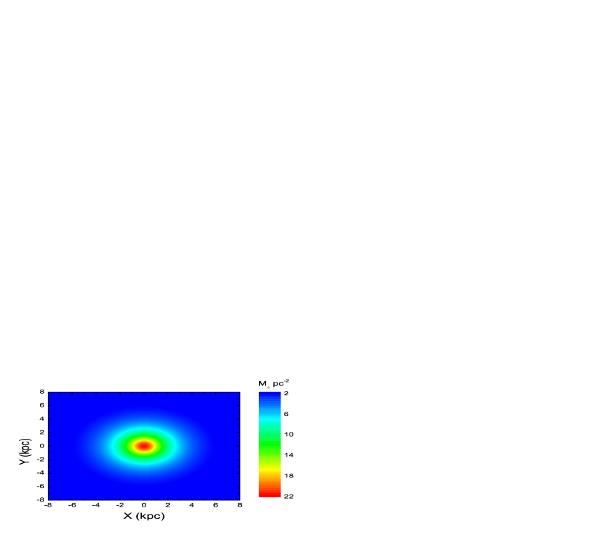
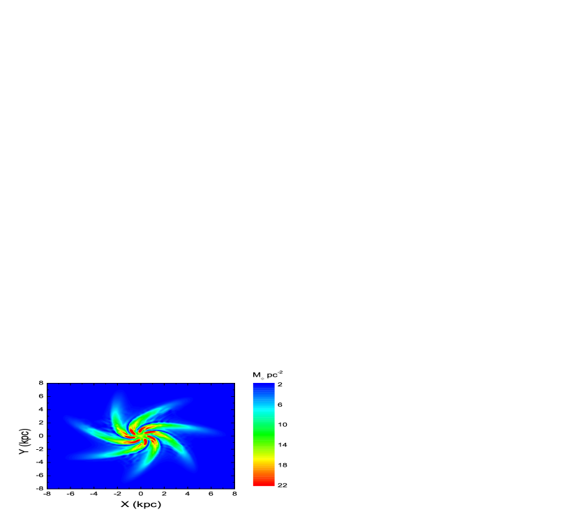
Figure 22: Evolution of the column density (in $M_{\odot}pc^{-2}$) in model 4. The evolution times are 0 Myr (top-left), 100 Myr (top-right), 150 Myr (bottom-left) and 200 Myr (bottom-right).

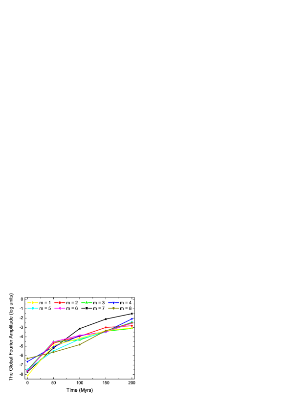
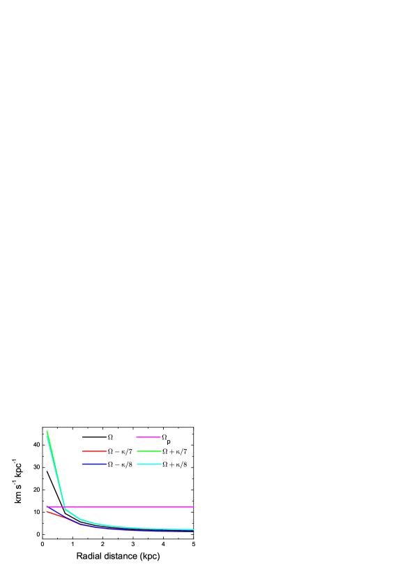
Figure 23: Top: Time evolution of the global Fourier amplitudes in model 4. Bottom: radial profiles of $\Omega$, $\Omega_{p}$, $\Omega\pm\kappa/7$, and $\Omega\pm\kappa/8$. The intersection of $\Omega_{p}$ with $\Omega-\kappa/8$ marks the position of the inner Lindblad resonance for the $m=8$ mode.

Finally, in Figure (22) we show the development a seven-armed spiral pattern in model 4. This model has the smallest ratio of the disk mass to the DM mass among all models, $\xi=0.0236$. The time evolution of the global Fourier amplitudes shown in the upper panel of Figure (23) confirms that the $m=7$ mode is the fastest growing one. The bottom panel in Figure (23) demonstrates that the ILR for the $m=7$ is absent, while the ILR for the $m=8$ mode is present in model 4.

To conclude, our numerical code behaves in accordance with the theoretical expectations on this difficult test problem. We find that the systems with a smaller disk to DM mass ratio develop patterns with a higher number of spiral arms, which may have interesting implications for the studies of global non-axisymmetric structures in disk galaxies.

CONCLUSIONS

In this paper, we present a new approach for constructing a low-dissipation numerical scheme to simulate hydrodynamic flows in astrophysics. The method is based on a combination of the operator-splitting method, Godunov method, and piecewise-parabolic method on the local stencil. Our numerical method was tested on an extensive suite of hydrodynamic test problems. The performance of the method is demonstrated on a global astrophysical problem showing the development of a multi-arm spiral structure in a gravitationally unstable gaseous galactic disk in accordance with the swing amplification theory.

Our numerical method has the following advantages: 1) High-order numerical solution on continuous functions and low-dissipation numerical solution on discontinuous functions, 2) absence of artificial viscosity and flux limiters, 3) Gallilean-invariance of numerical solutions, 4) guaranteed non-decrease of entropy, 5) extensibility on other numerical hyperbolic systems, 6) simplicity of parallel implementation on hybrid and classic supercomputers, 7) high scalability.

Main disadvantages of the numerical method is a rather simple finite-difference scheme for the time derivative. In future works, we will focus on extending our numerical method to include the moments of collisionless Boltzmann equations to describe the dynamics of stars and dark matter in galaxies [7, 48, 51, 63, 64]. We also plan to include the magnetohydrodynamics effects. This model will be used for numerical modelling of galactic dynamics and evolution of protostellar disks [65]. We also plan to implement our numerical scheme on GPU supercomputer (SSCC SB RAS) [48] and on Intel Xeon Phi supercomputers (JSCC RAS) [49]. In addition, the numerical method can be used for non astrophysical problem, for example to model explosion welding problems [50].

Appendix. The construction of piecewise-parabolic functions

In this section, we construct a piecewise-parabolic function $q(x)$ on a regular mesh with step $h$. For simplicity, we choose a spacial domain $[x_{i-1/2},x_{i+1/2}]$. A parabola on this local domain has the following form [22]:

$$q(x)=q_{i}^{L}+\xi\left(\bigtriangleup q_{i}+q_{i}^{(6)}(1-\xi)\right),$$ (65)

where $q_{i}$, $q_{i}^{L}$, and $q_{i}^{R}$ are defined at the cell center, at the left-hand side and right-hand side interface, respectively, $\xi=(x-x_{i-1/2})h^{-1}$, $\bigtriangleup q_{i}=q_{i}^{L}-q_{i}^{R}$ and $q_{i}^{(6)}=6(q_{i}-1/2(q_{i}^{L}+q_{i}^{R}))$. We note that equation (65) satisfies the conservation law

$$q_{i}=h^{-1}\int_{x_{i-1/2}}^{x_{i+1/2}}q(x)dx.$$

For calculating the values of $q_{i}^{R}=q_{i+1}^{L}=q_{i+1/2}$, we used a 4-th order interpolation function of the following form:

$$q_{i+1/2}=1/2(q_{i}+q_{i+1})-1/6(\delta q_{i+1}-\delta q_{i}),$$

where $\delta q_{i}=1/2(q_{i+1}-q_{i-1})$.

Below we present an algorithm for constructing the local parabola $q(x)$. The input for this algorithm are the values of $q_{i}$ at the cell centers. The output of the algorithm are the local parabolas on each domain $[x_{i-1/2},x_{i+1/2}]$.

Step 1. At the first step, we construct $\delta q_{i}=1/2(q_{i+1}-q_{i-1})$. To do this, we use the values of $q_{i+1},q_{i-1}$ at the neighbouring cells. To eliminate possible extrema on the local parabola, we must modify the formula for $\delta q_{i}$ as follows:

$$\delta_{m}q_{i}=\left\{\begin{array}[]{c}\min(|\delta q_{i}|,2|q_{i+1}-q_{i}|,2|q_{i}-q_{i-1}|){\rm sgn}(\delta q_{i}),(q_{i+1}-q_{i})(q_{i}-q_{i-1})>0\\ 0,(q_{i+1}-q_{i})(q_{i}-q_{i-1})\leq 0\end{array}\right..$$

After computing $\delta_{m}q_{i}$, we find the values on the boundary as:

$$q_{i}^{R}=q_{i+1}^{L}=q_{i+1/2}=1/2(q_{i}+q_{i+1})-1/6(\delta_{m}q_{i+1}-\delta_{m}q_{i}).$$

Step 2. At the second step, we can construct parabolas $q(x)$ on the local domain as follows:

$$\bigtriangleup q_{i}=q_{i}^{L}-q_{i}^{R},$$

$$q_{i}^{(6)}=6(q_{i}-1/2(q_{i}^{L}+q_{i}^{R})).$$

In the case of non-monotonic local parabolas, we must reconstruct the values on the boundary $q_{i}^{L},q_{i}^{R}$ as:

$$q_{i}^{L}=q_{i},q_{i}^{R}=q_{i},(q_{i}^{L}-q_{i})(q_{i}-q_{i}^{R})\leq 0,$$

and

$$q_{i}^{L}=3q_{i}-2q_{i}^{R},\bigtriangleup q_{i}q_{i}^{(6)}>(\bigtriangleup q_{i})^{2},$$

$$q_{i}^{R}=3q_{i}-2q_{i}^{L},\bigtriangleup q_{i}q_{i}^{(6)}<-(\bigtriangleup q_{i})^{2}.$$

Step 3. At the third step, we recalculate every parabola on the local domain using the following equations:

$$\bigtriangleup q_{i}=q_{i}^{L}-q_{i}^{R},$$

$$q_{i}^{(6)}=6(q_{i}-1/2(q_{i}^{L}+q_{i}^{R})).$$

This step completes the construction of local parabolas on each domain $[x_{i-1/2},x_{i+1/2}]$. These parabolas may be discontinuous on the cell boundaries. In this case, we must solve the Riemann problem. In the classic piecewise-parabolic method parabolas are continuous, but in the PPML methods local parabolas may be discontinuous, which is an important feature of the latter method.

To construct the Riemann solver, we must integrate $q(x)$ along the characteristics $\pm\lambda t$ to the left and to the right from the cell interface. The result can be written in the following form:

$$q_{L}(-\lambda t)=(\lambda t)^{-1}\int_{x_{i+1/2}-\lambda t}^{x_{i+1/2}}q(x)dx=q_{i}^{R}-\frac{\lambda t}{2h}\left(\bigtriangleup q_{i}-q_{i}^{(6)}\left(1-\frac{2\lambda t}{3h}\right)\right),$$

$$q_{R}(\lambda t)=(\lambda t)^{-1}\int_{x_{i+1/2}}^{x_{i+1/2}+\lambda t}q(x)dx=q_{i}^{L}+\frac{\lambda t}{2h}\left(\bigtriangleup q_{i}+q_{i}^{(6)}\left(1-\frac{2\lambda t}{3h}\right)\right).$$

These values can be used in Equations (33),  (34) and (41) for $v_{L}(\pm\lambda t)$, $v_{R}(\pm\lambda t)$, $p_{L}(\pm\lambda t)$, $p_{R}(\pm\lambda t)$, $f_{L}(-|\lambda|t)$ and $f_{R}(|\lambda|t)$.

Figure 11: Results of the two interacting blast waves problem.

Figure 13: The problem double Mach reflection of a strong shock. The isolines of density for computational mesh of $840\times 240$ grid zones

Figure 20: Evolution of the column density (in $M_{\odot}pc^{-2}$) in model 3. The evolution times are 0 Myr (top-left), 100 Myr (top-right), 250 Myr (bottom-left) and 360 Myr (bottom-right).

Table 1: Behavior of Poisson solver on meshes with different resolution

The mesh size	The relative error
$16^{3}$	4.799777e-005
$32^{3}$	2.978253e-006
$64^{3}$	1.862059e-007
$128^{3}$	1.164110e-008
$256^{3}$	7.278760e-010
$512^{3}$	4.548964e-011
$1024^{3}$	2.843139e-012

Table 2: Initial state of the shock tube problem

N	$\rho_{L}$	$v_{L}$	$p_{L}$	$\rho_{R}$	$v_{R}$	$p_{R}$	$x_{0}$	$t$
1	1	0	1	0.125	0	0.1	0.5	0.2
2	1	-2	0.4	1	2	0.4	0.5	0.15
3	1	0	1000	1	0	0.01	0.5	0.012

Table 3: Model parameters

Model	$M_{\rm disk}$	$\xi=M_{\rm disk}/M_{\rm DM}$	$Q_{\rm min}$	$T$	dominant mode
	($10^{10}M_{\odot}$)			K
1	0.217	0.0434	3.912	$10^{4}$	—
2	0.854	0.1708	1.109	$10^{4}$	2
3	0.334	0.0668	1.122	$10^{4}$	4
4	0.118	0.0236	1.243	$2\times 10^{3}$	7

References

- [1] O. Agertz, et al., Fundamental differences between SPH and grid methods, Monthly Notices of the Royal Astronomical Society. 380, 963-978, (2007).
- [2] E.J. Tasker, et al., A test suite for quantitative comparison of hydrodynamic codes in astrophysics, Monthly Notices of the Royal Astronomical Society. 390, 1267-1281, (2008).
- [3] I. Kulikov, G. Lazareva, A. Snytnikov and V. Vshivkov, Supercomputer Simulation of an Astrophysical Object Collapse by the Fluids-in-Cell Method, Lectures Notes of Computer Science. 5698, 414-422, (2009).
- [4] R. Attwood, S. Goodwin and A. Whitworth, Adaptive smoothing length in SPH, Astronomy & Astrophysics. 464, 447-450, (2007).
- [5] D. Sijacki and V. Springel, Physical Viscosity in Smoothed Particle Hydrodynamics Simulations of Galaxy Clusters, Monthly Notices of the Royal Astronomical Society. 371, 1025-1046, (2006).
- [6] J. Wadsley, G. Veeravalli and H. Couchman, On the treatment of entropy mixing in numerical cosmology, Monthly Notices of the Royal Astronomical Society 387, 427-438, (2008).
- [7] N. Mitchell, E. Vorobyov and G. Hensler, Collisionless Stellar Hydrodynamics as an Efficient Alternative to N-body Methods, Monthly Notices of the Royal Astronomical Society. 428, 2674-2687, (2013).
- [8] J. Murphy and A. Burrows, BETHE-Hydro: An Arbitrary Lagrangian-Eulerian Multidimensional Hydrodynamics Code for Astrophysical Simulations, The Astrophysical Journal Supplement Series. 179, 209-241, (2008).
- [9] V. Springel, E pur si muove: Galilean-invariant cosmological hydrodynamical simulations on a moving mesh, Monthly Notices of the Royal Astronomical Society. 401, 791-851, (2010).
- [10] I. Kulikov, PEGAS: Hydrodynamical code for numerical simulation of the gas components of interacting galaxies, Book Series of the Argentine Astronomical Society. 4, 91-95, (2013).
- [11] V. Vshivkov, G. Lazareva and I. Kulikov, A modified fluids-in-cell method for problems of gravitational gas dynamics, Optoelectronics, Instrumentation and Data Processing. 43, 530-537, (2007).
- [12] V. Vshivkov, G. Lazareva, A. Snytnikov, I. Kulikov and A. Tutukov, Hydrodynamical code for numerical simulation of the gas components of colliding galaxies, The Astrophysical Journal Supplement Series. 194, 47, (2011).
- [13] Vshivkov, V., Lazareva, G., Snytnikov, A., Kulikov, I., Tutukov, A., Computational methods for ill-posed problems of gravitational gasodynamics, Journal of Inverse and Ill-posed Problems. 19, 151-166, (2011).
- [14] A. Tutukov, G. Lazareva and I. Kulikov, Gas Dynamics of a Central Collision of Two Galaxies: Merger, Disruption, Passage, and the Formation of a New Galaxy, Astronomy Reports. 55, 770-783, (2011).
- [15] A. Kurganov and E. Tadmor, New High-Resolution Central Schemes for Nonlinear Conservation Laws and Convection-Diffusion Equation, J. Comput. Phys. 160, 214-282, (2000).
- [16] B. Van Leer, Towards the Ultimate Conservative Difference Scheme, V. A Second Order Sequel to Godunov’s Method, J. Comput. Phys. 32, 101-136, (1979).
- [17] S. Jin and Z. Xin, The Relaxation Schemes for Systems of Conservation Laws in Arbitrary Space Dimensions, Communications on Pure and Applied Mathematics. 48, 235-276, (1995).
- [18] G.-S. Jiang and C.-W. Shu, Efficient Implementation of Weighted ENO Schemes J. Comput. Phys. 126, 202-228, (1996).
- [19] D. Balsara and C.-W. Shu, Monotonicity Preserving Weighted Essentially Non-oscillatory Schemes with Increasingly High Order of Accuracy, J. Comput. Phys. 160, 405-452, (2000).
- [20] D. Balsara, T. Rumpf, M. Dumbser and C.-D. Munz, Efficient, high accuracy ADER-WENO schemes for hydrodynamics and divergence-free magnetohydrodynamics, J. Comput. Phys. 228, 2480-2516, (2009).
- [21] A. Henrick, T. Aslam and J. Powers, Mapped weighted essentially non-oscillatory schemes: Achieving optimal order near critical points, J. Comput. Phys. 207, 542-567, (2005).
- [22] P. Collela and P.R. Woodward, The Piecewise Parabolic Method (PPM) Gas-Dynamical simulations, J. Comput. Phys. 54, 174-201, (1984).
- [23] N. Watersona and H. Deconinck, Design principles for bounded higher-order convection schemes – a unified approach, J. Comput. Phys. 224, 182-207, (2007).
- [24] M. Popov and S. Ustyugov, Piecewise parabolic method on local stencil for gasdynamic simulations, Computational Mathematics and Mathematical Physics. 47, 1970-1989, (2007).
- [25] M. Popov and S. Ustyugov, Piecewise parabolic method on a local stencil for ideal magnetohydrodynamics, Computational Mathematics and Mathematical Physics. 48, 477-499, (2008).
- [26] D. Balsara and D. Spicer, Maintaining Pressure Positivity in Magnetohydrodynamic Simulations, J. Comput. Phys. 148, 133–148, (1999).
- [27] D. Ryu, J. Ostriker, H. Kang and R. Cen, A cosmological hydrodynamic code based on the total variation diminishing scheme, The Astrophysical Journal. 414, 1-19, (1993).
- [28] V. Springel and L. Hernquist, Cosmological smoothed particle hydrodynamics simulations: the entropy equation, Monthly Notices of the Royal Astronomical Society. 333, 649-664, (2002).
- [29] S. Godunov and I. Kulikov, Computation of Discontinuous Solutions of Fluid Dynamics Equations with Entropy Nondecrease Guarantee, Computational Mathematics and Mathematical Physics. 54, 1012-1024, (2014).
- [30] P. Roe, Approximate Riemann solvers, parameter vectors, and difference solvers, J. Comput. Phys. 135, 250-258, (1997).
- [31] D. Balsara, Multidimensional HLLE Riemann solver: Application to Euler and magnetohydrodynamic flows, J. Comput. Phys. 229, 1970-1993, (2010).
- [32] D. Balsara, A two-dimensional HLLC Riemann solver for conservation laws: Application to Euler and magnetohydrodynamic flows, J. Comput. Phys. 231, 7476-7503, (2012).
- [33] D. Balsara, M. Dumbser and R. Abgrall, Multidimensional HLLC Riemann solver for unstructured meshes – With application to Euler and MHD flows, J. Comput. Phys. 261, 172-208, (2014).
- [34] D. Balsara, Multidimensional Riemann problem with self-similar internal structure. Part I –- Application to hyperbolic conservation laws on structured meshes, J. Comput. Phys. 277, 163-200, (2014).
- [35] D. Balsara and M. Dumbser, Multidimensional Riemann problem with self-similar internal structure. Part II – Application to hyperbolic conservation laws on unstructured meshes, J. Comput. Phys. 287, 269-292, (2015).
- [36] D. Balsara, Three dimensional HLL Riemann solver for conservation laws on structured meshes: Application to Euler and magnetohydrodynamic flows, J. Comput. Phys. 295, 1-23, (2015).
- [37] D. Balsara and M. Dumbser, Divergence-free MHD on unstructured meshes using high order finite volume schemes based on multidimensional Riemann solvers, J. Comput. Phys. 299, 687-715, (2015).
- [38] W. Boscheri, D. Balsara and M. Dumbser, Lagrangian ADER-WENO finite volume schemes on unstructured triangular meshes based on genuinely multidimensional HLL Riemann solvers, J. Comput. Phys. 267, 112-138, (2014).
- [39] W. Boscheri, D. Balsara, and M. Dumbser, High-order ADER-WENO ALE schemes on unstructured triangular meshes-application of several node solvers to hydrodynamics and magnetohydrodynamics. International journal for numerical methods in fluids. 76, 737-778, (2014).
- [40] G. Bryan, et al., ENZO: An Adaptive Mesh Refinement Code for Astrophysics, The Astrophysical Journal Supplement Series. 211, 19 (2014).
- [41] D. Clarke, On the Reliability of ZEUS-3D, The Astrophysical Journal Supplement Series. 187, 119-134, (2010).
- [42] D. Balsara, Self-adjusting, positivity preserving high order schemes for hydrodynamics and magnetohydrodynamics, J. Comput. Phys. 231, 7504-7517, (2012).
- [43] X. Zhang and C.-W. Shu, On positivity-preserving high order discontinuous Galerkin schemes for compressible Euler equations on rectangular meshes, J. Comput. Phys. 229, 8918-8934, (2010).
- [44] M. Frigo and S. Johnson, The Design and Implementation of FFTW3, Proceedings of the IEEE. 93, 216-231, (2005).
- [45] V. Goloviznin and S. Karabasov, Nonlinear correction of Cabaret scheme, Mathematical Modelling Journal. 10, 107-123, (1998).
- [46] C.-W. Shu, Total-Variation-Diminishing time discretizations, SIAM Journal on Scientific and Statistical Computing. 9, 1073-1084, (1988).
- [47] C.-W. Shu and S. Osher, Efficient implementation of essentially non-oscillatory shock-capturing schemes, J. Comput. Phys. 77, 439-471, (1988).
- [48] I. Kulikov, GPUPEGAS: A New GPU-accelerated Hydrodynamic Code for Numerical Simulations of Interacting Galaxies, The Astrophysical Journal Supplements Series. 214, 12, (2014).
- [49] I. Kulikov, I. Chernykh, A. Snytnikov, B. Glinskiy and A. Tutukov, AstroPhi: A code for complex simulation of dynamics of astrophysical objects using hybrid supercomputers, Computer Physics Communications. 186, 71-80, (2015).
- [50] S. Godunov, S. Kiselev, I. Kulikov and V. Mali, Numerical and experimental simulation of wave formation during explosion welding, Proceedings of the Steklov Institute of Mathematics. 281, 12-26, (2013).
- [51] E. Vorobyov and Ch. Theis, Boltzmann moment equation approach for the numerical study of anisotropic stellar discs, Monthly Notices of the Royal Astronomical Society. 373, 197-208, (2006).
- [52] P. Woodward and P. Colella, The Numerical Simulation of Two-Dimensional Fluid Flow with Strong Shocks, J. Comput. Phys. 54, 115-173, (1984).
- [53] S.-H. Yoon, C. Kim and K.-H. Kim, Multi-dimensional limiting process for three-dimensional flow physics analyses, J. Comput. Phys. 227, 6001-6043, (2008).
- [54] A.V. Aksenov, Linear Differential Relations Between Solutions of the Class of Euler-Poisson-Darboux Equations, Journal of Mathematical Sciences. 130, 4911-4940, (2005).
- [55] A. Toomre, On the gravitational stability of a disk of stars, The Astrophysical Journal. 139, 1217-1238, (1964).
- [56] A. Nelson, W. Benz, F. Adams and D. Arnett, Dynamics of Circumstellar Disks, The Astrophysical Journal. 502, 342–371, (2008).
- [57] V. Polyachenko, E. Polyachenko and A. Strel’nikov, Stability criteria for gaseous self-gravitating disks, Astronomy Letters. 23, 483-491, (1997).
- [58] E. Vorobyov, S. Recchi and G. Hensler, Self-gravitating equilibrium models of dwarf galaxies and the minimum mass for star formation, Astronomy & Astrophysics 543, A129, (2012).
- [59] E. Athanassoula, The spiral structure of galaxies, Physics Reports. 114, 319-403 (1984).
- [60] P. Goldreich and D. Lynden-Bell II. Spiral arms as sheared gravitational instabilities, Monthly Notices of the Royal Astronomical Society. 130, 125-158, (1965).
- [61] A. Toomre, What amplifies the spirals, In ”The Structure and Evolution of Normal Galaxies” Fall S. M., Lynden-Bell D., eds, Cambridge University Press, Cambridge. 283, (1981).
- [62] J. Binney and S. Tremaine, Galactic Dynamics, Princeton Univ. Press, Princeton, NJ. 904 (2008).
- [63] E. Vorobyov and Ch. Theis, Shape and orientation of stellar velocity ellipsoids in spiral galaxies, Monthly Notices of the Royal Astronomical Society. 383, 817-830, (2008).
- [64] V. Protasov, A. Serenko, V. Nenashev, I. Kulikov and I. Chernykh, High-Performance Computing in Astrophysical Simulations, Journal of Physics: Conference Series. 681, 012022, (2016).
- [65] E. Vorobyov, D. Lin and M. Guedel, The effect of external environment on the evolution of protostellar disks, Astronomy & Astrophysics. 573, A5, (2015).
(a)
(b)
(c)