A mean-field approach applied for the ferromagnetic spin-1 Blume-Capel model

Abstract

We applied a mean-field approach associated to Monte Carlo simulations in order to study the spin-1 ferromagnetic Blume-Capel model in the square and the linear lattice. This new technique, which we call MFT-MC, determines the molecular field as the magnetization response of a Monte Carlo simulation. The resulting phase diagram is qualitatively correct, in contrast to effective-field approximations, in which the first-order line is not perpendicular to the anisotropy axis at low temperatures. Thermodynamic quantities, as the entropy and the specific heat curves can be obtained so as to analyze the nature of the phase transition points. Also, the possibility of using larger sizes constitutes an improvement regarding other mean-field approximations that use clusters.

PACS numbers: 64.60.Ak; 64.60.Fr; 68.35.Rh

I Introduction

In general, many-body systems with interactions are very difficult to solve exactly. A way to overcome this difficulty is by approaching the many-body problem by a one-body problem, in which a mean-field replaces the interactions affecting the body. This idea is applied to the ferromagnetic Ising Model (see reference kadanoff1 ). In the most simple mean-field approach, the nearest-neighbor interactions affecting each spin $S_{i}$ are replaced in such a way that $S_{i}$ now interacts with an effective field given by $zJ\langle S_{i}\rangle$, where $z$ is the coordination number, $J$ the exchange constant, and $\langle S_{i}\rangle$ is the thermal average of the spin $i$. This is the so called ”Weiss mean-field approach” weiss . Nevertheless, it neglects the spin correlations, and it leads the transition temperature $T_{c}$ as well as the values of the critical exponents away from the exact values ($T_{c}=zJ/k_{B}$, for all dimensions). However, for the one-dimensional case, the Ising model lacks of a phase transition at finite temperature, but Weiss’ approach wrongly predicts that $T_{c}=2J/k_{B}$.

A further step for improving the solution of this problem, is to use the proposal of Hans Bethe, which consists in considering that a central spin should interact with all its nearest-neighbor spins forming a cluster bethe . Then, that cluster would interact to an effective -field that approaches the next-nearest-neighbor spins surrounding the cluster. Thus, this improvement gives $T_{c}=2J/k_{B}\ln(z/(z-2))$, which not only betters the approximation of the critical temperatures, but leads correctly to $T_{c}=0$, for the one-dimensional case. In this way, the correlations between the spins has been included to some degree by considering a cluster of spins interacting with its nearest-neighbors.

The mean-field approach used in Ising-like models with finite-size clusters is based on the following Hamiltonian splitting:

$$\mathcal{H}=\mathcal{H}_{c}+\mathcal{H}_{v},$$ (1)

where $\mathcal{H}_{c}$ corresponds to the energy that is composed of spin variables of the finite cluster, whereas $\mathcal{H}_{v}$, corresponds to the energy of the neighborhood, whose spins do not belong to the central sites of the finite cluster. In the canonical ensemble, the calculation of mean values of the spin variables $G_{c}$ belongs to the subspace $n_{c}$ of the finite cluster, and it is computed by the following procedure:

$$\left\langle G_{c}\right\rangle =\frac{TrG_{c}\exp(-\beta\mathcal{H})}{Tr\exp(-\beta\mathcal{H})}$$

$$=\left\langle\frac{Tr_{n_{c}}G_{c}\exp(-\beta\mathcal{H}_{c})}{Tr_{n_{c}}\exp(-\beta\mathcal{H}_{c})}\right\rangle,$$ (2)

This equation is exact if $\left[\mathcal{H}_{c},\mathcal{H}_{v}\right]=0$.

The great merit of Eq.(2), is that we can solve the model of the infinite system by using a finite system in the subspace $n_{c}$. Various approximation methods use Eq.(2) as a starting point. One of them is the effective-field theory (EFT) proposed by Honmura and Kaneyoshi Kaneyoshi for solving the spin-1/2 ferromagnetic system. Sousa et al. Jsousa1 ; Jsousa2 ; Jsousa3 ; Jsousa4 applied EFT so as to treat different magnetic models with competing interactions. Recently, Viana et al. Viana developed a mean-field proposal for spin models, denominated effective correlated mean-field (ECMF), based on the following ansatz:

$$\sigma_{j}=\lambda_{m}\left\langle S_{c}\right\rangle,$$ (3)

where $\sigma_{j}$ are the neighbors of the central spins of the finite cluster, $\left\langle S_{c}\right\rangle$ is the mean of the spin variable of the cluster, and $\lambda_{m}$ is a term exhibiting the behavior of a molecular parameter. There are many ways of determining the parameter $\lambda_{m}$. In the present work we use Eq. (3) by proposing that $\lambda_{m}$ be the mean response of the spins of a Monte Carlo simulation (SMC), thus we make use of the following expression:

$$\lambda_{m}\equiv\left\langle S_{j}\right\rangle_{MC}$$ (4)

where

$$\left\langle S_{j}\right\rangle_{MC}=\frac{1}{p}\overset{p}{\underset{k=1}{\sum}}\left(\frac{1}{Q}\left|\overset{Q}{\underset{j=1}{\sum}}S_{j}\right|\right)_{k},$$ (5)

where $p$ is the number of Monte Carlo steps of the traditional Metropolis algorithm, and $Q$ is the total number of sites $S_{j}$ used in SMC. In what follows, we call this new mean-field Monte Carlo technique as MFT-MC.

The aim of this proposal is the improvement of the results obtained by other mean-field techniques, but we believe that the main advantage of our mean-field proposal is the simplicity in which we can treat the first-order phase transitions. Accordingly, in this work, we implemented this proposal in the spin-1 Blume-Capel model in the linear chain and in the square lattice.

We remark that the Blume-Capel model ($\bf BC$) Blume ; Capel is one of the most suitable models for studying magnetic systems from the point of view of the Statistical Mechanics. This model and its generalization, the Blume-Emery-Griffiths model, ($\bf BEG$) was proposed to describe the $\lambda$ transition in $\bf{}^{4}He-^{3}He$ mixtures beg as well as ordering in a binary alloy rys ; hint . Furthermore, its applications also include the description of ternary fluids mukamel1974 ; furman1977 , solid-liquid-gas mixtures and binary fluids laj1975 ; siv1975 , micro-emulsions schick1986 ; gompper1990 , ordering in semiconducting alloys newman1983 ; newman1991 and electron conduction models kivelson1990 . Indeed, the BC model is found in many works using different lattices, spin degrees, including disorder and different Statistical Mechanic techniques Grollau ; Kimel ; Xavier ; Plascak ; zaim2008 ; Polat1 ; Polat2 ; Zhang ; Kopec .

The BC model is represented by the following Hamiltonian:

$$\mathcal{H}_{N}=-J\overset{N}{\underset{i\neq j}{\sum}}S_{i}^{z}S_{j}^{z}+D\overset{N}{\underset{i\neq j}{\sum}}\left(S_{i}^{z}\right)^{2},$$ (6)

where $J$ is the ferromagnetic coupling between the spins $S_{i}^{z}=\pm 1,0$ of the lattice and $D$ is the anisotropy parameter. When the value of $D$ increases from zero, the energy levels $\mathcal{H}_{N}$ tend to the state $S_{i}^{z}=0$, in such a way that when $D>D_{c}$ all the spins take the value $S_{i}^{z}=0$ and the system suffers a first-order phase transition, i.e., the system goes from the ordered state ($S_{i}^{z}=\pm 1$) to the state ($S_{i}^{z}=0$) through a jump discontinuity. The critical value $D_{c}$ can be determined by equating the energy of the order and disordered states, i.e.,

$$\mathcal{H}_{N}(S_{j}^{z}=\pm 1)=\mathcal{H}_{N}(S_{j}^{z}=0).$$ (7)

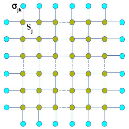
Figure 1: Scheme for sites located on a square lattice, where we have the central sites (yellow color) and neighboring sites (blue color).

Therefore, the BC model provides us a phase diagram with a a tricritical point separating a second and a first-order frontier that divides the ferromagnetic order (F) and the paramagnetic region (PM). This rich critical behavior qualifies the BC model for representing different phase transitions, and our purpose is to apply the MFT-MC method in it. The phase diagram of the BC model with equivalent-neighbor interactions can be seen in Fig.1 of reference octavio , which is qualitatively the same for dimensions greater than one.

II Implementation of the technique

In order to study the ferromagnetic model in the square lattice, we use Fig.1 as a reference. In this figure we may see that $\sigma_{k}$ represents the neighbors of the central sites $S_{j}^{z}$, which compose the finite cluster of $N_{c}$ sites. So, the Hamiltonian of the BC model is conveniently written in the following form:

$$\mathcal{H}_{N_{c}}=-J\overset{N_{c}}{\underset{i\neq j}{\sum}}S_{i}^{z}S_{j}^{z}+D\overset{N_{c}}{\underset{i\neq j}{\sum}}\left(S_{i}^{z}\right)^{2}-J\overset{N_{c}}{\underset{j=1}{\sum}}\overset{n_{j}}{\underset{k=1}{\sum}}\sigma_{k}S_{j}^{z},$$ (8)

where $J$ is the ferromagnetic coupling factor, $n_{j}$ is the number of spins $\sigma_{k}$ interacting with $S_{j}$ and $D$ is the anisotropy parameter. Note that Eq. (8) can be rewritten as follows:

$$-\beta\mathcal{H}_{N_{c}}=K\overset{N_{c}}{\underset{i\neq j}{\sum}}S_{i}^{z}S_{j}^{z}-Kd\overset{N_{c}}{\underset{i\neq j}{\sum}}\left(S_{i}^{z}\right)^{2}+\overset{N_{c}}{\underset{j=1}{\sum}}C_{j}S_{j}^{z},$$ (9)

where $K=\beta J$ ($\beta=1/k_{B}T$), $d=D/J$ and

$$C_{j}=K\overset{n_{j}}{\underset{k=1}{\sum}}\sigma_{k}.$$ (10)

In the present work the ansatz given in Eq. (3) is our fundamental assumption, so

$$C_{j}=n_{j}\lambda_{m}K\left\langle S_{c}^{z}\right\rangle.$$ (11)

In this work we considered clusters containing $N_{c}=2,4,9,25,36,49,64,81,100$ central sites. Thus, we have the following relations:

$$\text{ }N_{c} =2\text{: }C_{j}=3\lambda_{m}K\left\langle S_{c}^{z}\right\rangle.$$ (12)

$$\text{ }N_{c} =4\text{: }C_{j}=2\lambda_{m}K\left\langle S_{c}^{z}\right\rangle.$$ (13)

$$\text{ }N_{c} \geq 9\text{: }C_{j}=2\lambda_{m}K\left\langle S_{c}^{z}\right\rangle\text{ or }C_{j}=\lambda_{m}K\left\langle S_{c}^{z}\right\rangle\text{ or }C_{j}=0.\text{\ }$$ (14)

The magnetization per particle $m=\left\langle S_{c}^{z}\right\rangle$ of the magnetic system is given by the following definition:

$$\left\langle S_{c}^{z}\right\rangle=\frac{1}{N_{c}}\frac{Tr_{\Omega}\left(\overset{N_{c}}{\underset{j=1}{\sum}}S_{j}^{z}\right)\exp(-\beta\mathcal{H}_{N_{c}})}{Z_{N_{c}}},$$ (15)

where the partition function in the space of sites $S_{j}^{z}$ is given by

$$Z_{N_{c}}=Tr_{\Omega}\exp(-\beta\mathcal{H}_{N_{c}}).$$

An important issue is the thermodynamic treatment of the spin system, accordingly, we use the free energy given by the following equation:

$$\phi=-\frac{1}{N_{c}}t\ln\left(Z_{N_{c}}\right)+\gamma m^{2},$$ (16)

where $t=k_{B}T/J$ is the reduced temperature and $\gamma$ is a parameter to be determined. At the equilibrium, the free energy is minimized, thus:

$$\frac{\partial\phi}{\partial m}=f_{m}\equiv 0\text{,}$$ (17)

where the function $f_{m}$ stands for the equation of state given by

$$f_{m}=m-\left\langle S_{c}^{z}\right\rangle,$$ (18)

and we can determine the parameter $\gamma$ by using Eq. (17).

III Results

We firstly obtained the phase diagram of the BC model in the plane $d$-$t$ in a square lattice, based on the considerations of the previous section. In Fig. (2) we show the phase diagram for clusters containing $N_{c}=2$ (in (a)) and $N_{c}=16$ (in (b)) central sites. We faced the computational problem of solving the model for big clusters, inasmuch as the number of accessible states corresponds to $3^{N_{c}}$ states. For instance, for $N_{c}=16$ and $N_{c}=100$ sites, we have accessible states of order $10^{7}$ and $10^{47}$, respectively, which are huge numbers. Accordingly, for clusters of sizes $N_{c}>16$, we prefer only to calculate the critical temperature $t_{c}$, for $d=0$, and the coordinates of the tricritical point $P(d_{t},t_{t})$.

In order to plot the frontiers in Fig. (2), we used $L=80$, for the size of the square lattice, and $p=10^{7}$ Monte Carlo steps in the simulation so as to obtain the molecular parameter $\lambda_{m}$. It should be noted that, for $L>80$ and $p>10^{7}$, the results of the physical parameters obtained in the mean-field approach are just the same. In this figure we may observe that the critical value of the anisotropy corresponds to $d_{c}=2.0$, for $t\rightarrow 0$, which agrees with exact results obtained when equating the energy of the ordered state $(S_{j}^{z}=\pm 1)$, with the energy of the disordered one ($S_{j}^{z}=0$), for a finite system of $N$ sites, i.e.,

$$d_{c}=\frac{q}{2},$$ (19)

where $q$ is the coordination number of the lattice. The black circle represents the tricritical point that separates the second-order and the first-order frontier. We observe that the critical temperature $t_{c}$ decreases as the size of the cluster $N_{c}$ increases. The first-order frontier correctly falls perpendicularly to the anisotropy axis, however, in general, effective-field results do not reproduce this feature of the first-order frontier (see the IEFT curve in Figure 5 of reference Polat ).

In Table 1 we present the values of $t_{c}$, obtained for each cluster size $N_{c}$, where we compare the results of this work using MFT-MC with the mean-field approximation that uses clusters (MFT), where $\lambda_{m}=1$, in this case. We remark that Yüksel et al. Polat obtained $t_{c}\simeq 1.690$, by using a Metropolis Monte Carlo simulation, whereas Silva et al. Plascak obtained $t_{c}\simeq 1.714$ using Wang-Landau sampling. In references Beale and Xavier we have $t_{c}\simeq 1.695$ and $t_{c}\simeq 1.681$, respectively. We may observe that the results obtained by the MFT-MC approach are close to the SMC values when the cluster size is increased. Nevertheless, if compared with the MFT results, $t_{c}$ is better estimated by the MFT-MC method, regarding the SMC results as a reference.

The calculations of the tricritical points $P(d_{t},t_{t})$ through the MFT-MC technique are shown in Table 2. We see that when the cluster size $N_{c}$ is increased, the values of the critical anisotropy $d_{t}$ approach the values $d_{t}=1.966(2)$ and $d_{t}=1.974$ obtained by the Monte Carlo simulations of references Plascak and Polat , respectively. In what the value $t_{t}$ respects, the tendency of the convergence is closer to that of reference Polat , which gives $t_{t}=0.753$, within their effective-field approach (IEFT).

The coordinates of the tricritical point were determined through a Landau expansion,

$$\phi(d,t)=\overset{\infty}{\underset{p=0}{\sum}}A_{p}(d,t)m^{p}.$$ (20)

From this equation, we are interested in solving the following system of equations

$$A_{2}(d_{t},t_{t}) = 0$$ (21)

$$A_{4}(d_{t},t_{t}) = 0,$$ (22)

in order to obtain the tricritical point. So, we may note that

$$A_{p}=-\frac{t}{N_{c}}\frac{1}{Z_{N_{c}}}\left(\frac{\partial^{p}Z_{N_{c}}}{\partial m^{p}}\right)_{m=0}+\left(\frac{\partial^{p}}{\partial m^{p}}\left(\gamma m^{2}\right)\right)_{m=0}$$ (23)

corresponds to the equation that determines the coefficients $a_{p}$.

In Fig. (3) and Fig. (4) we can see the behavior of the magnetization and the entropy, respectively. These are related to the phase diagram shown in Fig. (2), for $N_{c}=16$. Thus, the magnetization and the entropy curves, as functions of the temperature, were used to exemplify the first-order phase transition happening for $d=1.9$, and the second-order phase transition, for $d=0.9$. In Fig. (3) we may observe that the magnetization falls down to zero continuously for the second-order phase transition (see curve (a)), while it suffers of jump discontinuity for the first-order one (see curve (b)). The study of the entropy per site is developed from the following expression:

$$s=-\left(\frac{\partial\phi}{\partial T}\right)_{v},$$ (24)

where $v$ means that all the other variables must be fixed in this differentiation. In Fig. (4) the entropy exhibits an inflection point at the second-order transition (in curve (b)), nevertheless, we may see a discontinuity at the first-order transition being characterized by $\Delta s\neq 0$ (see curve (a)), thus indicating the presence of a latent heat equal to $T\Delta s$, at the corresponding transition temperature. In the limit of high temperatures ($t\rightarrow\infty$) the entropy is $s(t\rightarrow\infty)=\ln\left(3\right)$, where the number $3$ is the number of accessible states for each spin of a spin-1 system. This result is correct in the canonical formalism.

In order to study other lattices, we particularly consider the criticality of an uni-dimensional lattice. In Fig. (5) we have the scheme of an uni-dimensional lattice used in modeling the mean-field theory. The terms $C_{j}$ correspond to the following expressions for each size $N_{c}$:

$$\text{ }N_{c} =1\text{: }C_{j}=2\lambda_{m}Km.$$ (25)

$$\text{ }N_{c} =2\text{: }C_{j}=\lambda_{m}Km.$$ (26)

$$\text{ }N_{c} \geq 3\text{: }C_{j}=\lambda_{m}Km\text{ or }C_{j}=0.\text{ }$$ (27)

In Table 3 we show the results of the critical temperature $t_{c}$ for the uni-dimensional lattice, running $p=10^{7}$ Monte Carlo steps so as to get the molecular parameter $\lambda_{m}$. We may observe that when the size of the cluster $N_{c}$ is increased the value of the critical temperature tends to zero, which is correct for an uni-dimensional system with nearest-neighbor interactions. So, though the convergence to the zero temperature is slow with $N_{c}$, it proves that the MFT-MC works in the lowest dimension.

IV Conclusions

In this paper we study the ferromagnetic spin-1 Blume-Capel model with nearest-neighbor interactions, within a mean-field approach, which uses the magnetization response of a Monte Carlo simulation, as the molecular field. We call this new approach as MFT-MC. For the bi-dimensional case, we implemented the model in the square lattice. The results show that when the size of the cluster $N_{c}$ increases, the values of the critical temperature $t_{c}$ (for null anisotropy) tend to $1.690$, which is the Monte Carlo estimation of Yüksel et al. Polat (see Table 1).

Another important result is related to the estimation of the tricritical point $P(d_{t},t_{t})$ in comparison with the results of Silva Plascak and YükselPolat (see Table 2). Our MFT-MC values of $d_{t}$ reasonably agree with the results of the Monte Carlo simulations, as $N_{c}$ increases, whereas $t_{t}$ tends to the effective-field (IEFT) result developed in reference Polat .

In order to test our MFT-MC approach, we applied it to the uni-dimensional case, where we can verify through Table 3, that the critical temperature converges to zero for larger sizes. This shows that the MFT-MC works well for uni-dimensional and bi-dimensional lattices. Furthermore, this proposal allows an analysis of the thermodynamic properties after obtaining the entropy and the specific heat curves. On the other hand, the possibility of working with larger sizes constitutes an advantage for analyzing the finite-size effects. Finally, we hope that this new approaching technique can be applied satisfactorily in other models and lattices .

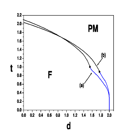
Figure 2: Phase diagram of the BC model obtained by our new approching technique called MFT-MC. The black circles represent tricritical points separating first- and second-order frontier lines. Frontiers (a) and (b) were produced with $N_{c}=2$ and $N_{c}=16$, respectively.

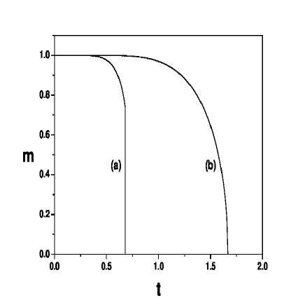
Figure 3: The behavior of the magnetization for $N_{c}=16$, showing the case of first- and second-order phase transitions where in (a) $d=1.9$ and in (b) $d=0.9$, respectively.

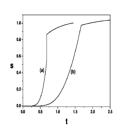
Figure 4: The behavior of the entropy, for $N_{c}=16$, showing the case of first- and second-order phase transitions using (a) $d=1.9$ and (b) $d=0.9$, respectively.

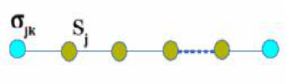
Figure 5: Scheme for sites located on a unidimensional lattice, where we have the central sites (yellow color) and neighboring sites (blue color).

Table 1: Critical temperatures obtained for different cluster sizes using the MFT-MC and a MFT approach, in which $\lambda_{m}=1$ in Eq.(3).

$N_{c}$	2	4	9	16	25	36	49	64	81	100
MFT-MC	$2.097\$	$2.075\$	$\ 2.054\$	$\ 2.033\$	$1.989\$	$\ 1.966\$	$\ 1.942$	$\ 1.931$	$1.916\ \$	$\ 1.883\$
MFT	$2.551$	$2.406\ \$	$2.309\ \$	$\ \ 2.259$	$2.117\ \$	$2.073\ \$	$2.015\ \$	$1.994\ \$	$1.983\$	$1.966\$

Table 2: Values of the tricritical points $P(d_{t},t_{t})$ obtained by the MFT-MC approach, for different cluster sizes. The points $(d_{t}=1.966(2),t_{t}=0.609(3))$ and $(d_{t}=1.974,t_{t}=0.56)$ obtained in references Plascak and Polat , can be reference points for comparison.

$N_{\mathbf{c}}$	$2$	$4$	$9$	$16$	$25$	$36$	$49$	$64$	$81$	$100$
$\ d_{t}$	$1.548$	$1.631$	$1.702$	$1.772$	$1.814$	$1.855$	$1.871$	$1.892$	$1.922$	$1.941$
$t_{t}$	$1.002$	$0.982$	$0.933$	$0.891$	$0.862$	$0.841$	$0.813$	$0.772$	$0.754$	$0.725$

Table 3: Critical temperatures for unidimensional lattice obtained for various cluster sizes using MFT-MC technique.

$N_{\mathbf{c}}$	4	20	50	100	200	500	1000	2000
$t_{c}$	0.614	0.4870	0.423	0.381	0.345	0.239	0.145	0.002