Parallelized Structures for MIMO FBMC under Strong Channel Frequency Selectivity

Abstract

A novel architecture for MIMO transmission and reception of filterbank multicarrier (FBMC) modulated signals under strong frequency selectivity is presented. The proposed system seeks to approximate an ideal frequency-selective precoder and linear receiver by Taylor expansion, exploiting the structure of the analysis and synthesis filterbanks. The resulting architecture is implemented by linearly combining conventional MIMO linear transceivers, which are applied to sequential derivatives of the original filterbank. The classical per-subcarrier precoding/linear receiver configuration is obtained as a special case of this architecture, when only one stage is fixed at both transmitter and receiver. An asymptotic expression for the resulting intersymbol/intercarrier (ISI/ICI) distortion is derived assuming that the number of subcarriers grows large. This expression can in practice be used in order to determine the number of parallel stages that need to be implemented in the proposed architecture. Performance evaluation studies confirm the substantial advantage of the proposed scheme in practical frequency-selective MIMO scenarios.

I Introduction

The increasing demand for high data rate wireless services has recently motivated a renewed interest in spectrally efficient signalling methodologies in order to overcome the current spectrum scarcity. In this context, filterbank multicarrier (FBMC) modulations have become very strong candidates to guarantee an optimum spectrum usage while maintaining the nice processing properties of multicarrier signals, such as reduced complexity equalization. Unlike cyclic-prefix OFDM (CP-OFDM), FBMC modulations do not require the use of a cyclic prefix and can be constructed via spectrally contained pulse shaping architectures. This significantly increases the spectral efficiency of the system, improves the spectral localization of the transmitted signal and reduces the need for guard bands. FBMC modulations can be combined with multi-antenna MIMO technology in order to boost the link system capacity, leading to an extremely high spectral efficiency.

Even though several alternative FBMC modulation formats have been proposed over the last few years, the most interesting one from the point of view of spectral efficiency remains to be FBMC based on offset QAM (FBMC/OQAM) [1, 2]. This modulation is constructed via a critically sampled uniformly spaced filterbanks modulated by real-valued symbols. Given the fact that there is no CP and since the filterbanks are critically sampled, FBMC/OQAM achieves the largest possible spectral efficiency in the whole class of FBMC modulations. Furthermore, by conveniently selecting the prototype filters at the transmit and receive side, one can perfectly recover the transmitted symbols at the receiver in the presence of a noiseless frequency flat channel. For this reason, this modulation is widely considered as the most prominent FBMC modulation.

A second important class of FBMC modulations are typically referred to as Filtered Multi Tone (FMT) or FBMC/QAM [3, 4]. The idea behind these modulations consists in directly modulating complex QAM symbols instead of real-valued ones, avoiding again the introduction of a CP. The approach is clearly more versatile than FBMC/OQAM and since the signalling is carried out on complex symbols, the modulation operative becomes very similar to classical CP-OFDM. However, it can be seen that if the filterbank is critically sampled it is not possible to perfectly recover the transmitted symbols, even in the presence of a noiseless frequency flat channel. For this reason, FBMC/QAM is typically implemented using oversampled filterbanks, which clearly reduce the spectral efficiency of the system. As a consequence of using oversampled filterbanks, the different constituent filters have little overlap in the frequency domain, which minimizes potential problems in terms of inter-carrier interference (ICI) with respect to FBMC/OQAM. For all these reasons, FBMC/QAM is today a valid alternative employed in commercial systems such as the professional mobile radio system TETRA Enhanced Data System (TEDS) [6]. However, due to the introduction of redundancy (oversampling) in the transmit/receive filterbanks, FBMC/QAM can only achieve a portion of the spectral efficiency of a classical FBMC/OQAM modulation.

Several other alternative FBMC modulations have been proposed in the literature, although they typically rely on the introduction of CP, which simplifies the equalization but clearly incurs in a significant spectral loss. This CP is not needed in FBMC modulations, because under relatively mild channel frequency selectivity the channel response can be assumed to be approximately flat within each subcarrier band. Hence, a single-tap per-subcarrier weighting is in principle sufficient to equalize the system, as it is the case in CP-OFDM. Unfortunately, in the presence of strong channel frequency selectivity, the channel can no longer be approximated as flat within each subcarrier pass band, and FBMC modulations require more sophisticated equalization systems (see e.g. [7] and references therein for a review of FBMC equalization techniques). In practical terms, if the receiver keeps using a single-tap per-subcarrier equalizer in the presence of a highly frequency-selective channel, its output will appear contaminated by a residual distortion superposed to the background noise. In FBMC/QAM modulations, this distortion will eminently be related to the inter-symbol-interference (ISI) caused by the channel within each subband. In FBMC/OQAM modulations, the strong overlap between the different subband filters will result in both ICI and ISI at the output in the presence of a frequency-selective channel. Consequently, the effect of channel frequency selectivity becomes more problematic in FBMC/OQAM modulations, a fact that has prevented a more widespread acceptance of this modulation in spite of its clear superiority in terms of spectral efficiency.

This residual distortion under channel frequency selectivity is much more devastating in MIMO transmissions, basically due to a superposition effect of the multiple parallel antennas/streams [8, 9, 10]. This incremental distortion effect in MIMO contexts has traditionally been mitigated using complex receiver strategies, such as sophisticated equalization architectures [11, 12, 13], or algorithms based on successive interference cancellation [14, 15, 13]. More recent approaches have additionally considered the optimization of the transmitter architecture in order to mitigate the effect of the channel frequency selectivity. For example, [16] considers the optimization of the precoder/linear receiver pair in order to achieve spatial diversity while minimizing the residual distortion at the output of the receiver. A related approach can be found in [17, 18], where a polynomial-based (multi-tap) SVD precoder is applied together with an equivalent multi-tap equalizer at the receiver.

Here we take an approach similar to the one in [19] and propose a general architecture that can be used to implement multiple MIMO transceivers (precoder plus linear receiver) in highly frequency-selective channels. Our approach is substantially different from the one in [16, 17, 18], because rather than focusing on a particular objective to optimize the transceiver, the proposed architecture provides a general framework that can be used to construct a variety of MIMO transceivers. On the other hand, the results in this paper generalize [19] in several important aspects, even under the SISO configuration. First, the approach in [19] considers the specific case where the transmitter does not apply any precoding/pre-equalization processing, while the receiver performs direct channel inversion. Here, we consider a much more general setting with a generic precoder/pre-equalizer at the transmitter together with the corresponding equalizer at the receiver. Second, the asymptotic performance analysis in [19] is based on the assumption that the prototype pulses are perfect reconstruction (PR) filters. Here, the analysis is generalized to the case where the prototypes are not necessarily PR, which is typically the case in practice. Finally, the analysis in [19] is only valid for finite impulse response (FIR) channel models. Here, the analysis is generalized to more general channel forms, not necessarily having finite impulse response.

Before going into the technical development, it is worth pointing out that the present study assumes linear, time invariant and perfectly estimated channel responses. These assumptions are not perfectly met in a practical situation, mainly because of the presence of amplifier nonlinearities, Doppler effects and the use of finite training sequences. Still, we assume that all these imperfections are negligible for the sake of analytical tractability. The detrimental effect of these nonidealities could in principle be reduced by increasing the cost of the power amplifier and by employing channel estimates are refreshed frequently enough and obtained with a sufficiently large training sequence. However, in practice these ideal conditions do not hold, and therefore some degradation in the performance should be expected. Previous analyses establish that the negative effect of these non-idealities in FBMC is similar to the one in CP-OFDM [20, 21, 22], which leads us to believe that the associated performance degradation will not be dramatic.

The rest of the paper is organized as follows. Section II presents the general MIMO signal model and the ideal frequency-selective transceiver that is considered in this paper and Section III presents the proposed parallel multi-stage approach for general FBMC systems. The asymptotic performance of the proposed MIMO architecture is analyzed in Section IV for general FBMC/OQAM modulations under the assumption that the number of subcarriers grows large. Finally, Section V provides a numerical evaluation of the multi-stage technique and Section VI concludes the paper. All technical derivations have been relegated to the appendices.

II Signal model

We consider a MIMO system with $N_{T}$ transmit and $N_{R}$ receive antennas. Let $\mathbf{H}(\omega)$ denote an $N_{R}\times N_{T}$ matrix containing the frequency response of the MIMO channels, so that the $\left(i,j\right)$th entry of $\mathbf{H}(\omega)$ contains the frequency response between the $j$th transmit and the $i$th receive antennas. We assume that the MIMO system is used for the transmission of $N_{S}$ parallel signal streams, $1\leq N_{S}\leq\min\left\{N_{R},N_{T}\right\}$, which correspond to FBMC modulated signals. More specifically, we will denote by $\mathbf{s}(\omega)$ an $N_{S}\times 1$ column vector that contains the frequency response of the signal transmitted at each of the $N_{S}$ parallel streams. Hence, each entry of the vector $\mathbf{s}(\omega)$ is the Fourier transform of a FBMC modulated symbol stream.

Let us assume that the transmitter applies a frequency-dependent linear precoder, which will be denoted by the $N_{T}\times N_{S}$ matrix $\mathbf{A}(\omega)$. The signal transmitted through the $N_{T}$ transmit antennas can be expressed as

$$\mathbf{x}(\omega)=\mathbf{A}(\omega)\mathbf{s}(\omega)$$ (1)

where $\mathbf{x}(\omega)$ is an $N_{T}\times 1$ column vector containing the frequency response of the transmitted signal. On the other hand, let $\mathbf{y}(\omega)$ denote an $N_{R}\times 1$ column vector containing the frequency response of the received signals in noise, namely

$$\mathbf{y}(\omega)=\mathbf{H}(\omega)\mathbf{x}(\omega)+\mathbf{n}(\omega)$$

where $\mathbf{n}(\omega)$ is the additive Gaussian white noise. We assume that the receiver estimates the transmitted symbols by linearly transforming the received signal vector $\mathbf{y}(\omega)$. More specifically, we consider a certain $N_{R}\times N_{S}$ receive matrix $\mathbf{B}(\omega)$ so that the symbols are estimated by

$$\mathbf{\hat{s}}(\omega)=\mathbf{B}^{H}(\omega)\mathbf{y}(\omega).$$

The whole ideal frequency-selective transceiver chain is implemented in Fig. 1 for a FBMC-modulated system. The number of subcarriers is fixed to be even, and will be denoted by $2M$.

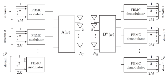
Figure 1: Ideal implementation of a frequency selective precoder $\mathbf{A}(\omega)$ and a linear receiver $\mathbf{B}(\omega)$ in a FBMC modulation system with $2M$ subcarriers.

The main problem with the MIMO architecture presented in Fig. 1 comes from the fact that, in practice, the frequency-dependent matrices $\mathbf{A}(\omega),$ $\mathbf{B}(\omega)$ need to be implemented using real filters. However, these filters have very large (or even infinite) impulse responses, which may be difficult to implement in practice. This can partly be solved in multicarrier modulations, as long as it can be assumed that the frequency selectivity is not severe, so that the channel response is approximately flat at on each subcarrier pass band. When this is the case, one can construct the MIMO precoder/receiver operations by applying the matrices $\mathbf{A}(\omega_{k}),$ $\mathbf{B}(\omega_{k})$ to each subcarrier stream, where here $\omega_{k}$ denotes the central frequency associated with the $k$th subcarrier. This is further illustrated in Fig. 2 for the particular case of $N_{T}=N_{R}=2$ antennas in a FBMC modulation transmission. Observe that the traditional (per-subcarrier) implementation in Fig. 2 is the result of changing the position of the precoder/linear receiver with respect to the FBMC modulator/demodulator in the ideal implementation.

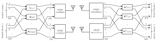
Figure 2: Traditional implementation of the frequecy-selective linear MIMO transmitter and receiver in multicarrier modulations, for the specific case of $N_{T}=2$ transmit antennas, $N_{R}=2$ receive antennas and $2M$ subcarriers.

As pointed out above, the traditional solution essentially relies on the fact that the channel frequency selectivity is mild enough to guarantee that each sub-carrier observes a frequency non-selective channel. However, under severe frequency selectivity, the system will suffer from a non-negligible distortion that will critically impair the performance of the MIMO system. This will be confirmed below, both analytically and via simulations. Next, we propose an alternative solution that tries to overcome this effect.

III Proposed approach

In this section we propose an alternative solution that, with some additional complexity, significantly mitigates the distortion caused by the channel frequency selectivity. We assume that the transmit and receive filterbanks are constructed by modulating a given prototype filter, which may be different at the transmit and receive sides. We will denote as $p[n]$ and $q[n]$ the real-valued impulse responses of the transmit and receive prototype pulses, with Fourier transforms respectively denoted by $P\left(\omega\right)$ and $Q\left(\omega\right)$, $\omega\in\mathbb{R}/2\pi\mathbb{Z}$. Hence, the frequency response of the $k$th filter in the transmit filterbank is assumed to be equal to $P\left(\omega-\omega_{k}\right)\,$ where $\omega_{1},\ldots,\omega_{2M}$ denote the subcarrier frequencies, assumed to be equispaced along the transmitted bandwidth, namely $\omega_{k}=2\pi\left(k-1\right)/\left(2M\right)$. The following approach could also be applied to the situation where $P\left(\omega\right)$ is different at each subcarrier, as well as in situations where these subcarriers are not equispaced. However we prefer to concentrate on the simpler case of uniform filterbanks to simplify the exposition.

Let us consider the combination of the FBMC transmission scheme with the frequency-selective MIMO precoder $\mathbf{A}(\omega)$. More specifically, consider the $k$th subcarrier associated with the $n_{S}$th MIMO signal stream that is sent through the $n_{T}$th transmit antenna. Assuming that the ideal frequency-selective precoder matrix $\mathbf{A}(\omega)$ is implemented (Fig. 1), this stream will effectively go through a transmit linear system with equivalent frequency response proportional to

$$P\left(\omega-\omega_{k}\right)\left\{\mathbf{A}(\omega)\right\}_{n_{T},n_{S}}.$$

The traditional (per-subcarrier) implementation of this precoder is based on the assumption that $\mathbf{A}(\omega)$ is almost flat along the bandwidth of $P\left(\omega-\omega_{k}\right)$ so that we can approximate

$$P\left(\omega-\omega_{k}\right)\left\{\mathbf{A}(\omega)\right\}_{n_{T},n_{S}}\simeq P\left(\omega-\omega_{k}\right)\left\{\mathbf{A}(\omega_{k})\right\}_{n_{T},n_{S}}.$$ (2)

In this situation, we can apply a constant precoder $\mathbf{A}(\omega_{k})$ to all the symbols that go through the $k$th subcarrier, which means that we can in practice change the order of precoder and FBMC modulator with respect to the ideal implementation (cf. Fig. 2). Under strong frequency selectivity of the ideal precoder $\mathbf{A}(\omega)$, the approximation in (2) does not hold anymore and a more accurate description of $\mathbf{A}(\omega)$ around $\omega_{k}$ is needed.

Assume that the entries of the precoding matrix $\mathbf{A}(\omega)$ are analytic functions of $\omega$, so that they are expressible as their Taylor series development around $\omega_{k}$, namely

$$\mathbf{A}(\omega)=\sum_{\ell=0}^{\infty}\frac{1}{\ell!}\mathbf{A}^{(\ell)}(\omega_{k})\left(\omega-\omega_{k}\right)^{\ell}$$

where $\mathbf{A}^{(\ell)}(\omega_{k})$ denotes the $\ell$th derivative of $\mathbf{A}(\omega)$ evaluated at $\omega=\omega_{k}$. The idea behind the classical precoder implementation in (2) and in Fig. 2 is to truncate this Taylor series development and to consider only its first term ($\ell=0$). Here, we suggest to go a bit further and consider the truncation of the above series representation to include its first $K_{T}$ terms ($T$ denoting transmit side), so that the transmitter filter has an effective frequency response equal to

$$\mathbf{A}(\omega)\simeq\sum_{\ell=0}^{K_{T}-1}\frac{1}{\ell!}\left(\omega-\omega_{k}\right)^{\ell}\mathbf{A}^{(\ell)}(\omega_{k}).$$ (3)

for $\omega$ sufficiently close to $\omega_{k}$. The main advantage of extending this truncation to the case $K_{T}>1$ comes from the fact that one can effectively implement the above filter by using $K_{T}$ parallel polyphase FBMC modulators corresponding to the $K_{T}$ sums in (3), so that each of the $K_{T}$ parallel precoders consists of single-tap per-subcarrier implementations. To see this, assume that the prototype pulse $p[n]$ is a sampled version of an original analog waveform $p(t)$ and define as $p^{(\ell)}[n]$ a sampled version of $p^{(\ell)}(t)$, namely the $\ell$th derivative of the analog waveform $p(t)$. These definitions will be more formally presented in Section IV. Then, under certain regularity conditions on the waveform $p(t)$, the Fourier transform of the sequence $p^{(\ell)}[n]$ can be approximated for large $M$ as

$$P^{(\ell)}\left(\omega\right)\simeq\left(2M\textnormal{j}\omega\right)^{\ell}P\left(\omega\right).$$ (4)

Hence, by conveniently rewriting (3), we see that we can approximate

$$P\left(\omega-\omega_{k}\right)\mathbf{A}(\omega)\simeq\\ \simeq\sum_{\ell=0}^{K_{T}-1}\frac{1}{\ell!}\left(\frac{-\textnormal{j}}{2M}\right)^{\ell}P^{(\ell)}\left(\omega-\omega_{k}\right)\mathbf{A}^{(\ell)}(\omega_{k}).$$ (5)

Now, observe that each term of the above sum has exactly the same form as the first order (single-tap per-subcarrier) precoder $P\left(\omega-\omega_{k}\right)\mathbf{A}(\omega_{k})$, replacing the actual precoder matrix $\mathbf{A}(\omega_{k})$ and the original prototype pulse $P\left(\omega\right)$ by their derivative-associated counterparts $\mathbf{A}^{(\ell)}(\omega_{k})$, $P^{(\ell)}\left(\omega\right)$. From all this, we can conclude that the $K_{T}$-term truncation of the ideal transmit precoder frequency response can be generated by combining a set of $K_{T}$ parallel conventional precoders. This is further illustrated in Fig. 3, where we represent the suggested implementation of the transmit precoder when the number of parallel stages was fixed to $K_{T}=2$ and the number of transmit antennas to $N_{T}=2$. We  have represented in red the additional stage that needs to be superposed to the original one (in black), which is the same as in Fig. 2

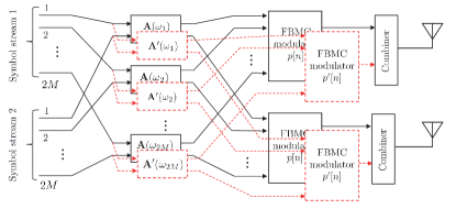
Figure 3: Proposed implementation of the frequecy-selective precoder for the specific case of $N_{T}=2$ transmit antennas and $N_{T}=2$ parallel stages.

We can follow the same approach in order to approximate the ideal frequency-selective linear receiver matrix $\mathbf{B}(\omega)$ in combination with the receive prototype pulse. Fig. 4 illustrates the proposed architecture for the simple case of $N_{R}=2$ receive antennas and $K_{R}=2$ parallel stages. From all the above, we can conclude that we can approximate the ideal frequency-selective precoder/linear receiver as depicted in Fig. 1 by simply increasing the number of parallel stages ($K_{T}$, $K_{R}$) that are implemented at the transmitter and at the receiver. In the following section we analyze the performance of the proposed transceiver architecture in terms of the residual ISI/ICI distortion at the output of the receiver.

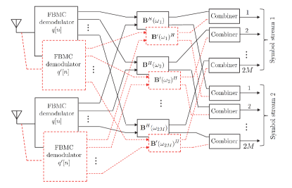
Figure 4: Proposed implementation of the frequecy-selective linear receiver for the specific case of $N_{R}=2$ receive antennas and $K_{R}=2$ parallel stages.

Let us now provide a more formal description of the proposed algorithm. Consider the transmission of $N$ complex-valued (QAM) multicarrier symbols through each of the $N_{S}$ MIMO streams. We will denote by $\mathbf{S}_{n}$, $n=1\ldots N_{S}$, a $2M\times N$ matrix that contains, at each of its columns, the multicarrier symbols that are transmitted through the $n$th MIMO stream. Let $\mathcal{Z}_{n}$, $n=1\ldots N_{S}$, denote the $2M\times\tilde{N}$ matrix of received samples corresponding to the reception of the $n$th MIMO stream (see further Fig. 1), where $\tilde{N}$ is the total number of non-zero received samples associated with the transmission of the $N$ multicarrier symbols (note that $\tilde{N}\geq N$ due to the memory of the filterbank). Observe that $\mathcal{Z}_{n}$ will inherently have contributions from all the symbol matrices $\mathbf{S}_{1},\ldots,\mathbf{S}_{N_{S}}$.

Remark 1

In what follows, given a general frequency-dependent quantity $X=X(\omega)$ we define $\Lambda\left(X\right)=\textnormal{diag}\left\{X(\omega_{1}),\ldots,X(\omega_{2M})\right\}$, i.e. a diagonal matrix containing the value of the function $X$ at the points $\omega_{1},\ldots,\omega_{2M}$. We will also write $H_{n_{R},n_{T}}=\left\{\mathbf{H}\left(\omega\right)\right\}_{n_{R},n_{T}}$, $A_{n_{T},n_{{}_{S}}}^{\left(\ell\right)}=A_{n_{T},n_{{}_{S}}}^{\left(\ell\right)}(\omega)=\left\{\mathbf{A}^{\left(\ell\right)}(\omega)\right\}_{n_{T},n_{{}_{S}}}$ and $B_{n_{R},n}^{\left(\ell\right)}=B_{n_{R},n}^{\left(\ell\right)}(\omega)=\left\{\mathbf{B}^{\left(\ell\right)}(\omega)\right\}_{n_{R},n}$. We will sometimes omit the dependence on $\omega$ in several frequency-dependent quantities when this fact is clear from the context.

Let us first provide a formal description of the receive signal samples $\mathcal{Z}_{n}$ associated with the $n$th MIMO symbol stream under the traditional per-subcarrier design in Figure 2. The $n_{S}$th symbol stream matrix $\mathbf{S}_{n_{S}}$ is precoded as $\Lambda\left(A_{n_{T},n_{{}_{S}}}\right)\mathbf{S}_{n_{S}}$ for each of the transmit antennas $n_{T}=1,\ldots,N_{T}$ and FBMC-modulated. The signal that is transmitted through the $n_{T}$ antenna goes through the channel $H_{n_{R},n_{T}}$ and is received by the $n_{T}$th antenna and FBMC-demodulated. We will denote by

$$\mathcal{Z}_{p,q}^{H_{n_{R},n_{T}}}\left(\Lambda\left(A_{n_{T},n_{{}_{S}}}\right)\mathbf{S}_{n_{S}}\right)$$ (6)

the $2M\times\tilde{N}$ matrix of received samples at the output of the corresponding FBMC demodulator, where $p,q$ are the prototype filters used at the transmitter and the receiver respectively. In order to recover the original symbols associated with the $n$th MIMO stream, a multiplicative coefficient is finally applied at this signal at the per-subcarrier level, so that the matrix in (6) is left multiplied by the diagonal $\Lambda\left(B_{n_{R},n}^{\ast}\right)$. The total received signal associated with the $n$th MIMO stream contains the contribution of all transmit streams, all transmit and all receive antennas, so that it can be expressed as

$$\mathcal{Z}_{n}=\sum_{n_{R}=1}^{N_{R}}\sum_{n_{T}=1}^{N_{T}}\sum_{n_{S}=1}^{N_{s}}\Lambda\left(B_{n_{R},n}^{\ast}\right)\mathcal{Z}_{p,q}^{H_{n_{R},n_{T}}}\left(\Lambda\left(A_{n_{T},n_{{}_{S}}}\right)\mathbf{S}_{n_{S}}\right)$$ (7)

plus some additive noise that we omit in this discussion. Now, if the channel and the precoder are sufficiently flat in the frequency domain, one may approximate (see Appendix A for a more formal exposition)

$$\mathcal{Z}_{p,q}^{H_{n_{R},n_{T}}}\left(\Lambda\left(A_{n_{T},n_{{}_{S}}}\right)\mathbf{S}_{n_{S}}\right)\simeq\Lambda\left(H_{n_{R},n_{T}}A_{n_{T},n_{{}_{S}}}\right)\mathcal{Y}_{p,q}\left(\mathbf{S}_{n_{S}}\right)$$ (8)

where $\mathcal{Y}_{p,q}\left(\mathbf{S}_{n_{S}}\right)=\mathcal{Z}_{p,q}^{1}\left(\mathbf{S}_{n_{S}}\right)$ is the matrix of FBMC-demodulated samples under an ideal SISO channel. Inserting this approximation into (7) we see that

$$\mathcal{Z}_{n}\simeq\sum_{n_{S}=1}^{N_{s}}\Lambda\left(\left\{\mathbf{B}^{H}\mathbf{HA}\right\}_{n,n_{S}}\right)\mathcal{Y}_{p,q}\left(\mathbf{S}_{n_{S}}\right).$$

If, additionally we force $\mathbf{B}^{H}\mathbf{HA=I}_{N_{S}}$, we will approximately have $\mathcal{Z}_{n}\simeq\mathcal{Y}_{p,q}\left(\mathbf{S}_{n}\right)$ which will be a close approximation of the transmitted symbols $\mathbf{S}_{n}$ if the prototype pulses are well designed.

Next, let us formulate the signal model under the proposed parallel multi-stage architecture, assuming that the number of parallel stages is $K_{T}$ at the transmit side and $K_{R}$ at the receive side. In order to define the derivatives of the prototype pulses of (4) in a formal manner, we make the following assumption:

$\mathbf{(As1)}$ The transmit and receive prototype pulses $p[n]$, $q[n]$ have length $2M\kappa$, where $\kappa$ is the overlapping factor. Furthermore, these pulses are obtained by discretization of smooth real-valued analog waveforms $p(t)$, $q(t)$, which are smooth functions $\mathcal{C}^{R+1}\left(\left[-T_{s}\kappa/2,T_{s}\kappa/2\right]\right)$, $R\geq K_{T}+K_{R}$, so that

$$p[n]=p\left(\left(n-\frac{2M\kappa+1}{2}\right)\frac{T_{s}}{2M}\right),\ n=1,\ldots,2M\kappa$$

and equivalently for $q[n]$, where $T_{s}$ is the multicarrier symbol period. Furthermore, the pulses $p(t)$, $q(t)$ and their $R+1$ sequential derivatives are null at the end-points of their support, namely at $t=\pm T_{s}\kappa/2$.

Thanks to the above assumption, we can define $p^{(r)}$ and $\,q^{(r)}$ as the sampled version of the $r$th derivative of $p(t)$ and $q(t)$ respectively, that is

$$p^{(r)}[n]=T_{s}^{r}p^{(r)}\left(\left(n-\frac{2M\kappa+1}{2}\right)\frac{T_{s}}{2M}\right),\ n=1,\ldots,2M\kappa$$

and equivalently for $q^{(r)}$. In order to construct the proposed multi-stage equalization system, we will assume that all quantities are sufficiently smooth in the frequency domain, namely:

$\mathbf{(As2)}$ The frequency-depending quantities $\mathbf{A}(\omega),\mathbf{B}(\omega)$ and $\mathbf{H}(\omega)$ are $\mathcal{C}^{R^{\prime}+1}\left(\mathbb{R}/2\pi\mathbb{Z}\right)$ functions, where $R^{\prime}>\left(2R+1\right)\left(R+1\right)$. Furthermore, these matrices are constructed so that $\mathbf{B}^{H}(\omega)\mathbf{H}(\omega)\mathbf{A}(\omega)=\mathbf{I}_{N_{s}}$.

Having established the definition of the time-domain derivative of the prototype pulses and the smoothness conditions on precoder and channel, we can now formulate the received signal model under the proposed parallel multi-stage precoding/receiving architecture. Let $\mathcal{Z}_{n}^{\left(\ell_{1},\ell_{2}\right)}$ be defined as the $2M\times\tilde{N}$ received signal matrix (equivalent to $\mathcal{Z}_{n}$), when transmitter and receiver employ the $\ell_{1}$th and $\ell_{2}$th parallel stages respectively. Keeping in mind that the $\ell$th parallel stage is constructed by replacing the prototype pulse and the precoder/decoder by their corresponding $\ell$th order derivatives, we can write

$$\mathcal{Z}_{n}^{\left(\ell_{1},\ell_{2}\right)}=\\ =\sum_{n_{{}_{S}}=1}^{N_{S}}\sum_{n_{R}=1}^{N_{R}}\sum_{n_{T}=1}^{N_{T}}\Lambda\left(B_{n_{R},n}^{\left(\ell_{2}\right)\ast}\right)\mathcal{Z}_{p^{(\ell_{1})},q^{(\ell_{2})}}^{H_{n_{R},n_{T}}}\left(\Lambda\left(A_{n_{T},n_{{}_{S}}}^{\left(\ell_{1}\right)}\right)\mathbf{S}_{n_{S}}\right)$$ (9)

which is basically the same equation as (7), but replacing $\left\{p,\mathbf{A}\right\}$ by $\left\{p^{(\ell_{1})},\mathbf{A}^{\left(\ell_{1}\right)}\right\}$ and $\left\{q,\mathbf{B}\right\}$ by $\left\{q^{(\ell_{2})},\mathbf{B}^{(\ell_{2})}\right\}$. The total received signal is therefore described by the linear combination of the signals that are transmitted and received by the multiple parallel stages, using the coefficients established in (5), namely

$$\mathcal{Z}_{n}=\sum_{\ell_{1}=0}^{K_{T}-1}\sum_{\ell_{2}=0}^{K_{R}-1}\frac{\left(-\textnormal{j}\right)^{\ell_{1}+\ell_{2}}}{\ell_{1}!\ell_{2}!\left(2M\right)^{\ell_{1}+\ell_{2}}}\mathcal{Z}_{n}^{\left(\ell_{1},\ell_{2}\right)}.$$ (10)

We claim that, assuming that precoder/receiver are constructed so that $\mathbf{B}^{H}(\omega)\mathbf{H}(\omega)\mathbf{A}(\omega)\mathbf{=I}_{N_{S}}$, the above signal model is a very good approximation of the multicarrier signal that would be received under frequency flat conditions, namely $\mathcal{Y}_{p,q}\left(\mathbf{S}_{n}\right)$. This will be more formally established in Section IV, where we provide an asymptotic characterization of the resulting distortion error. In order to provide these asymptotic results, we specifically focus on FBMC/OQAM modulations, which allow perfect orthogonality conditions under an ideal channel.

III-A Specificities of the FBMC/OQAM signal model

The conceptual form of the FBMC/OQAM modulator and demodulator is illustrated in Fig. 5. As mentioned above, this modulation is widely considered in the literature, thanks to the higher spectral efficiency with respect to other filterbank multicarrier modulations and the possibility of achieving perfect reconstruction of the transmitted symbols under perfect channel conditions [2]. It can be described as a uniform, critically sampled FBMC modulation scheme with different prototype pulses as the transmitter ($p$) and the receiver ($q$), where the transmitted symbols are drawn from a QAM modulation and staggered into an offset QAM (OQAM) format.

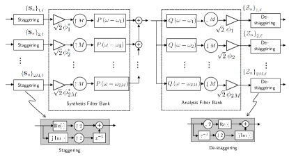
Figure 5: Basic form of a FBMC/OQAM modulator and demodulator. Here, $P(\omega)$ and $Q(\omega)$ are the transmit and receive prototype pulses, and $\phi_{k}=\text{e}^{-\textnormal{j}\pi(M+1)(k-1)/(2M)}$

.

As in the general description above, we consider that a total of $N$ complex QAM multicarrier symbols ($2N$ real-valued symbols) are sequentially transmitted through the $n$th stream, and let $\mathbf{S}_{n}$ denote a $2M\times 2N$ matrix that contains the symbols after the staggering operation. Each pair of columns of $\mathbf{S}_{n}$ corresponds to a complex multicarrier symbol, and will be denoted by $\mathbf{s}_{n}(\ell)$, $\ell=1,\ldots,N$. We will write $\mathbf{b}_{n}(\ell)=\textnormal{Re}\mathbf{s}_{n}(\ell)$ and $\mathbf{c}_{n}(\ell)=\textnormal{Im}\mathbf{s}_{n}(\ell)$, and we will denote as $\mathbf{B}_{n}$ and $\mathbf{C}_{n}$ the $2M\times N$ matrices obtained by stacking these vectors in columns. $\mathbf{b}_{n}(\ell)$ and $\mathbf{c}_{n}(\ell)$, so that $\mathbf{s}_{n}(\ell)=$ $\mathbf{b}_{n}(\ell)+\textnormal{j}\mathbf{c}_{n}(\ell)$. The signal matrix $\mathcal{Z}_{n}$ in (10) gathers the samples of the received signal associated with the $n$th MIMO substream before the de-staggering operation (see Fig. 5).

Following the notation in (8), under an ideal SISO channel and in the absence of precoder/receiver, the received samples matrix $\mathcal{Z}_{n}$ corresponding to the complex symbols $\mathbf{S}_{n}$ will be denoted by $\mathcal{Y}_{p,q}\left(\mathbf{S}_{n}\right)$. It can be seen [19] that matrix $\mathcal{Y}_{p,q}\left(\mathbf{S}_{n}\right)$ can be constrained to have dimensions  $2M\times\left(2N+2\kappa\right)$. The number of columns of this matrix corresponds to twice the number of transmitted multicarrier symbols ($2N$) plus some additional columns ($2\kappa$) that account for the tail effects of the prototypes $p,q$. From $\mathcal{Y}_{p,q}\left(\mathbf{S}_{n}\right)$, we can construct two matrices $\mathcal{Y}_{p,q}^{\text{odd}}\left(\mathbf{S}_{n}\right)$, $\mathcal{Y}_{p,q}^{\text{even}}\left(\mathbf{S}_{n}\right)$ which contain its even- and odd-numbered columns, so that

$$\mathcal{Y}_{p,q}\left(\mathbf{S}_{n}\right)=\mathcal{Y}_{p,q}^{\text{odd}}\left(\mathbf{S}_{n}\right)\otimes[0,1]+\mathcal{Y}_{p,q}^{\text{even}}\left(\mathbf{S}_{n}\right)\otimes[1,0]$$ (11)

where $\otimes$ is the Kronecker product. According to the FBMC/OQAM modulation, the original multicarrier symbols are retrieved by taking the real/imaginary parts of the appropriate columns of $\mathcal{Y}_{n}^{\text{odd}}\left(p,q\right)$ and $\mathcal{Y}_{n}^{\text{even}}\left(p,q\right)$, that is via a de-staggering operation

$$\mathbf{\hat{s}}_{n}(\ell)=\textnormal{Re}\left\{\mathcal{Y}_{p,q}^{\text{odd}}\left(\mathbf{S}_{n}\right)\right\}_{:,\ell+\kappa-1}+\textnormal{j}\textnormal{Im}\left\{\mathcal{Y}_{p,q}^{\text{even}}\left(\mathbf{S}_{n}\right)\right\}_{:,\ell+\kappa}\text{ .}$$ (12)

A exact expression of $\mathcal{Y}_{p,q}^{\text{odd}}\left(\mathbf{S}_{n}\right)$ and $\mathcal{Y}_{p,q}^{\text{even}}\left(\mathbf{S}_{n}\right)$ can be found in [19, (3)-(4)], see further (31) in Appendix A.

It is well known [2] that one can choose $p,q$ to meet some “bi-orthogonality” or perfect reconstruction (PR) conditions, which guarantee that $\mathbf{\hat{s}}_{n_{S}}(\ell)=\mathbf{s}_{n_{S}}(\ell)$ in (12). In order to formulate these conditions, let $\mathbf{P}$ and $\mathbf{Q}$ denote two $2M\times\kappa$ matrices obtained by arranging the original prototype pulse samples in columns. In other words, the $k$th row of $\mathbf{P}$ (resp. $\mathbf{Q}$) contains the $k$th polyphase component of the original pulse $p$ (resp. $q$). Next, consider two $2M\times\left(2\kappa-1\right)$ matrices $\mathcal{R}\left(p,q\right)$ and $\mathcal{S}\left(p,q\right)$ obtained as

$$\mathcal{R}\left(p,q\right) =\mathbf{P\circledast J}_{2M}\mathbf{Q}$$ (13)

$$\mathcal{S}\left(p,q\right) =\left(\mathbf{J}_{2}\otimes\mathbf{I}_{M}\right)\mathbf{P\circledast J}_{2M}\mathbf{Q}$$ (14)

where $\mathbf{\circledast}$ indicates row-wise convolution between matrices and $\mathbf{J}_{2M}$ is the anti-identity matrix of size $2M$. It is well known that one can impose PR conditions on the pulses $p$ and $q$ by imposing [19]

$$\mathbf{U}^{+}\mathcal{R}\left(p,q\right)=\mathcal{I},\quad\mathbf{U}^{-}\mathcal{S}\left(p,q\right)=\mathbf{0}$$ (15)

where $\mathbf{U}^{+}=\mathbf{I}_{2}\otimes\left(\mathbf{I}_{M}+\mathbf{J}_{M}\right)$, $\mathbf{U}^{-}=\mathbf{I}_{2}\otimes\left(\mathbf{I}_{M}-\mathbf{J}_{M}\right)$, and where $\mathcal{I}$ is a $2M\times\left(2\kappa-1\right)$ matrix with ones in its central column and zeros elsewhere. The above PR conditions can be significantly simplified when $p=q$ and assuming that the prototype pulses are symmetric or anti-symmetric in the time domain [2].

IV Performance analysis under FBMC/OQAM

Ideally, one would like to have $\mathcal{Z}_{n}$ as similar as possible to the signal of the output of the decimators in the FBMC demodulators when the ideal frequency-selective precoder and linear receiver are used (Fig. 1). In practice, however this only holds approximately, in the sense that $\mathcal{Z}_{n}$ in (10) can be written as

$$\mathcal{Z}_{n}=\mathcal{Y}_{p,q}\left(\mathbf{S}_{n}\right)+\mathcal{E}_{p,q}\left(\mathbf{S}_{n}\right)$$ (16)

for some error $\mathcal{E}_{p,q}\left(\mathbf{S}_{n}\right)$. More specifically, decomposing $\mathcal{Z}_{n}$ into $\mathcal{Z}_{n}^{\text{odd}}$ and $\mathcal{Z}_{n}^{\text{even}}$ as in (11), one would estimate the $\ell$th multicarrier symbol as

$$\mathbf{\hat{s}}_{n}(\ell)=\textnormal{Re}\left\{\mathcal{Z}_{n}^{\text{odd}}\right\}_{:,\ell+\kappa-1}+\textnormal{j}\textnormal{Im}\left\{\mathcal{Z}_{n}^{\text{even}}\right\}_{:,\ell+\kappa}\text{ .}$$ (17)

Two different sources of error will be present in this estimation of the symbols: an implementation error due to the frequency selectivity of the system, namely $\mathcal{E}_{p,q}\left(\mathbf{S}_{n_{S}}\right)$, plus a representation error which arises from the fact that the PR conditions in (15) may not hold. In this section, we characterize the behavior of the total resulting error by assuming that the number of subcarriers is asymptotically large ($M\rightarrow\infty$). The following additional assumptions will be needed in order to provide the corresponding result:

$\mathbf{(As3)}$ The transmitted complex symbols are drawn from a bounded constellation.

$(\mathbf{As4})$ The real and imaginary parts of the transmitted symbols are independent, identically distributed random variables with zero mean and power $P_{s}/2$.

Under these assumptions, it is possible to characterize the behavior of the residual distortion at the output of the receiver, assuming that the number of subcarriers is asymptotically high ($M\rightarrow\infty$). In order to formulate the result, we need some additional definitions, that are presented next. Given four integers $m,n,m^{\prime},n^{\prime}$, we define $\eta_{(m,n,m^{\prime},n^{\prime})}^{\left(+,-\right)}$ as the following pulse-specific quantity:

$$\eta_{(m,n,m^{\prime},n^{\prime})}^{\left(+,-\right)} =\frac{P_{s}}{2M}\textnormal{tr}\Bigg{[}\mathcal{R}\left(p^{(m)},q^{(n)}\right)\mathcal{R}^{T}\left(p^{(m^{\prime})},q^{(n^{\prime})}\right)\mathbf{U}^{+}$$

$$+\mathcal{S}\left(p^{(m)},q^{(n)}\right)\mathcal{S}^{T}\left(p^{(m^{\prime})},q^{(n^{\prime})}\right)\mathbf{U}^{-}\Bigg{]}$$

where $\mathcal{R(}$·,·$)$ and $\mathcal{S(}$·,·$)$ are defined in (13)-(14). The quantity $\eta_{(m,n)}^{\left(-,+\right)}$ is equivalently defined, but swapping $\mathbf{U}^{+}$ and $\mathbf{U}^{-}$ in the above equation. Let $\Psi_{K}^{\left(+,-\right)}$ denote a $2\times 2$ matrix constructed as

$$\Psi_{K}^{\left(+,-\right)}=\left[\begin{array}[c]{cc}\eta_{(K,0,K,0)}^{\left(+,-\right)}\mathbb{I}_{\left\{K_{T}=K\right\}}&\eta_{(K,0,0,K)}^{\left(+,-\right)}\mathbb{I}_{\left\{K_{R}=K_{T}\right\}}\\ \eta_{(K,0,0,K)}^{\left(+,-\right)}\mathbb{I}_{\left\{K_{R}=K_{T}\right\}}&\eta_{(0,K,0,K)}^{\left(+,-\right)}\mathbb{I}_{\left\{K_{R}=K\right\}}\end{array}\right]$$ (18)

where $\mathbb{I}_{\left\{\text{\textperiodcentered}\right\}}$ is the indicator function. Let $\Psi_{K}^{\left(-,+\right)}$ be constructed as $\Psi_{K}^{\left(+,-\right)}$ but changing all instances of $\left(+,-\right)$ for $\left(-,+\right)$.  The following quantities will take into account the fact that PR conditions may not hold

$$\delta =\frac{P_{s}}{2M}\textnormal{tr}\Bigg{[}\left(\mathcal{R}\left(p,q\right)-\frac{1}{2}\mathcal{I}\right)\left(\mathcal{R}\left(p,q\right)-\frac{1}{2}\mathcal{I}\right)^{T}\mathbf{U}^{+}$$

$$+\mathcal{S}\left(p,q\right)\mathcal{S}^{T}\left(p,q\right)\mathbf{U}^{-}\Bigg{]}$$

$$\mu_{(m,n)} =\frac{P_{s}}{2M}\textnormal{tr}\Bigg{[}\left(\mathcal{R}\left(p,q\right)-\frac{1}{2}\mathcal{I}\right)\mathcal{R}^{T}\left(p^{(m)},q^{(n)}\right)\mathbf{U}^{+}$$

$$+\mathcal{S}\left(p,q\right)\mathcal{S}^{T}\left(p^{(m)},q^{(n)}\right)\mathbf{U}^{-}\Bigg{]}$$

$$\tilde{\mu}_{\left(\ell,m\right)}^{(K)} =\sum_{j=K}^{\ell}\left(-1\right)^{j+K}\binom{\ell}{j}\binom{j-1}{K-1}\mu_{\left(j,m-j\right)}.$$

Indeed, observe that these two quantities are zero under the PR conditions in (15): clearly $\mathbf{U}^{-}\mathcal{S}\left(p,q\right)=\mathbf{0}$ whereas

$$\mathbf{U}^{+}\left(\mathcal{R}\left(p,q\right)-\frac{1}{2}\mathcal{I}\right)=\mathbf{U}^{+}\mathcal{R}\left(p,q\right)-\mathcal{I}=\mathbf{0.}$$

We will additionally need some channel-specific functions $\alpha_{n,n_{S}}^{(m,\ell)}\left(\omega\right)$, $\beta_{n,n_{S}}^{(m,\ell)}\left(\omega\right)$ and $\gamma_{n,n_{S}}\left(\omega\right)$, defined as

$$\alpha_{n,n_{S}}^{(m,\ell)} =\frac{\sqrt{2}\left(-\textnormal{j}\right)^{m}}{m!}\binom{m}{\ell}\left\{\left(\mathbf{B}^{H}\mathbf{H}\right)^{\left(m-\ell\right)}\mathbf{A}^{\left(\ell\right)}\right\}_{n,n_{S}}$$ (19)

$$\beta_{n,n_{S}}^{(m,\ell)} =\frac{\sqrt{2}\left(-\textnormal{j}\right)^{m}}{m!}\binom{m}{\ell}\left\{\mathbf{B}^{\left(\ell\right)H}\left(\mathbf{HA}\right)^{\left(m-\ell\right)}\right\}_{n,n_{S}}$$ (20)

$$\gamma_{n,n_{S}} =\frac{\sqrt{2}\left(-\textnormal{j}\right)^{K_{R}+K_{T}}}{K_{T}!K_{R}!}\left\{\mathbf{B}^{\left(K_{R}\right)H}\mathbf{HA}^{\left(K_{T}\right)}\right\}_{n,n_{S}}.$$ (21)

where we have omitted the dependence of all quantities on $\omega$ to ease the notation and where $\ell\leq m$. We have now all the ingredients to characterize the asymptotic distortion power associated with the $n$th parallel symbol stream observed at the $k$th subcarrier output of the FBMC/OQAM demodulator, which will be denoted by $P_{e}\left(k,n\right)$, $1\leq k\leq 2M$, $1\leq n\leq N_{S}$.

Theorem 1

Consider the linear parallelized MIMO FBMC system presented above, with $K_{T}\geq 1$ parallel stages at the transmitter and $K_{R}\geq 1$ parallel stages at the receiver. Let $\mathbf{\hat{s}}_{n}\left(\ell\right)$ be as defined in (17), i.e. as the estimate of $\mathbf{s}_{n}\left(\ell\right)$, the $\ell$th column vector of the complex-valued symbol matrix. Assume that $\mathbf{(As1)-(As4)}$ hold and let $K=\min\left(K_{T},K_{R}\right)$. Then for any $\ell\in\left\{\kappa,\ldots,N-\kappa\right\}$ one can write

$$\mathbb{E}\left[\left|\left\{\mathbf{\hat{s}}_{n}\left(\ell\right)\right\}_{k}-\left\{\mathbf{s}_{n}\left(\ell\right)\right\}_{k}\right|^{2}\right]=P_{e}\left(k,n\right)+o\left(M^{-2K}\right)$$

as $M\rightarrow\infty$. The term $P_{e}\left(k,n\right)$ can be decomposed in two terms, namely $P_{e}\left(k,n\right)=P_{e,1}\left(k,n\right)+P_{e,2}\left(k,n\right)$, with

$$P_{e,1}\left(k,n\right)=2\delta$$

$$-\sum_{m=K_{R}}^{2K}\frac{2\sqrt{2}}{\left(2M\right)^{m}}\sum_{\ell=K_{R}}^{m}\mu_{\left(0,m\right)}\textnormal{Re}\left(\beta_{n,n}^{(m,\ell)}\right)$$

$$-\sum_{m=K_{T}}^{2K}\frac{2\sqrt{2}}{\left(2M\right)^{m}}\sum_{\ell=K_{T}}^{m}\tilde{\mu}_{\left(\ell,m\right)}^{(K_{T})}\textnormal{Re}\left(\alpha_{n,n}^{(m,\ell)}\right)$$

$$+\frac{2\sqrt{2}}{\left(2M\right)^{2K}}\textnormal{Re}\gamma_{n,n}\mu_{(K,K)}\mathbb{I}_{\left\{K_{R}=K_{T}\right\}}$$

and

$$P_{e,2}\left(k,n\right) =\frac{1}{\left(2M\right)^{2K}}\sum_{n_{{}_{S}}=1}^{N_{S}}\textnormal{Re}^{T}\left[\xi_{n,n_{S}}^{(K,K)}\right]\Psi_{K}^{\left(+,-\right)}\textnormal{Re}\left[\xi_{n,n_{S}}^{(K,K)}\right]$$

$$+\frac{1}{\left(2M\right)^{2K}}\sum_{n_{{}_{S}}=1}^{N_{S}}\textnormal{Im}^{T}\left[\xi_{n,n_{S}}^{(K,K)}\right]\Psi_{K}^{\left(-,+\right)}\textnormal{Im}\left[\xi_{n,n_{S}}^{(K,K)}\right]$$

where $\xi_{n,n_{S}}^{(m,\ell)}\left(\omega\right)=\left[\alpha_{n,n_{S}}^{(m,\ell)}\left(\omega\right),\beta_{n,n_{S}}^{(m,\ell)}\left(\omega\right)\right]^{T}$ and where all the frequency-dependent quantities ($\alpha_{n,n_{S}}^{(m,\ell)},\beta_{n,n_{S}}^{(m,\ell)},\gamma_{n,n}$) are evaluated at $\omega=\omega_{k}$.

Proof:

See Appendix A. ∎

According to the above result, the inherent distortion of the FBMC/OQAM modulation can be asymptotically decomposed into two terms, $P_{e,1}\left(k,n\right)$ and $P_{e,2}\left(k,n\right)$. The first term basically accounts for the fact that the prototype pulses $p,q$ need not have PR conditions. It can readily be observed that this term is identically zero when the conditions in (15) hold. The second term $P_{e,2}\left(k,n\right)$ inherently describes the effect of the residual distortion caused by the channel frequency selectivity, even when PR conditions hold. This term essentially decays as $O\left(M^{-2K}\right)$ when $M\rightarrow\infty$, where $K$ is the minimum between transmit and receive parallel stages. This means that if both the transmit and the receive processing matrices are frequency-selective, it does not make much sense to increase the number of parallel stages at one side of the communications link beyond the number of stages at the other, since the asymptotic behavior will ultimately be dictated by the minimum between the two. The situation is different when only one of the matrices (either $\mathbf{A}(\omega)$ or $\mathbf{B}(\omega)$) is frequency-selective. In this case, the frequency flat matrix can be seen as its exact representation in Taylor series, which is equivalent to stating that the matrix is approximated using an infinite number of terms (most of which are zero), i.e. $K_{T}=\infty$ or $K_{R}=\infty$. In this situation, increasing the number of stages that implement the frequency-selective matrix will always have a beneficial effect.

On the other hand, one should also observe from the expression of $P_{e}\left(k,n\right)$ that the total residual distortion power that is observed at the $n$th receive symbol stream is an additive combination of the distortion associated with each of the transmit symbol streams (note the sum from $n_{S}=1$ to $N_{S}$ in the asymptotic expression for $P_{e,2}\left(k,n\right)$). This justifies the claim that general MIMO processing is very vulnerable to the presence of highly frequency-selective channels, since the higher the number of parallel streams, the higher the residual distortion power that will be observed at the output of the receiver. Furthermore, the expression of $P_{e}\left(k,n\right)$ provides a very convenient way of fixing the number of parallel stages at the transmitter and receiver ($K$) in order to guarantee a certain degree of performance. Given a triplet of channel, precoder and linear receiver ($\mathbf{A}(\omega)$, $\mathbf{H}(\omega)$ and $\mathbf{B}(\omega)$) one only needs to evaluate $P_{e}\left(k,n\right)\,$ in order to obtain the minimum $K$ that guarantees a sufficiently low distortion power.

Finally, it is worth pointing out that the asymptotic residual distortion expression presented in Theorem 1 generalizes the one obtained in [19] for SISO channels in different important aspects. Here, both transmit and receive frequency-selective processing structures are considered, whereas only receive processing (equalization) was assumed in [19]. Furthermore, the above expression of $P_{e}\left(k,n\right)$ above does not assume PR conditions on the prototype pulses, which was not the case in [19]. Section V shows that this asymptotic expression provides an extremely accurate description of the system behavior under severe channel frequency selectivity.

IV-A Computational Complexity and Latency

Contrary to multi-tap filter-based solutions that process the signal per subcarrier using a finite impulse response (FIR) filter, the proposed parallel multi-stage architecture incurs in no additional penalty in terms of latency. This is because all the constituent stages can be implemented in parallel, avoiding all the unnecessary delays of other multi-tap based filtering approaches. Note that the insertion of a multi-tap processor per subcarrier will generally incur in a latency increase proportional to the product between the number of taps and the number of subcarriers, which may not be tolerable in delay-critical applications.

As for the associated complexity of the proposed multi-stage architecture, we can evaluate it in terms of the total number of real-valued multiplications and sums. We will consider a transmit/receive filterbank implementation using an FFT-based polyphase architecture [2], assuming that the number of subcarriers is a power of $2$ and that the prototype pulses are symmetric in the time domain. Using the split-radix algorithm, one can implement an FFT by only using $2M\left(\log_{2}M-1\right)+4$ real-valued multiplications and $6M\log_{2}M+4$ real valued sums [23]. Using this together with the fact that the prototype pulse is real-valued and that each complex product can be implemented with $3$ real-valued multiplication plus $5$ real-valued sums, we can establish the total number of real-valued sums and multiplications of the multi-stage architecture given in Table I. In this table, we have disregarded the terms of order $o(M)$ and have also introduced the complexity of a MIMO multi-tap equalizer [12] for comparison purposes. These numbers will be used in the numerical analysis of the following section.

Algorithm	Real-valued products
Multi-stage (TX)	$2MK_{T}\left[N_{T}\log_{2}M+\left(\kappa+2\right)N_{T}+2N_{S}N_{T}\right]$
Multi-stage (RX)	$2MK_{R}\left[N_{R}\log_{2}M+\left(\kappa+2\right)N_{R}+3N_{R}N_{S}\right]$
Multi-tap (RX)	$2M\left[N_{R}\log_{2}M+\left(\kappa+2\right)N_{R}+3N_{S}N_{R}\left(N_{taps}+1\right)\right]$
Algorithm	Real-valued sums
Multi-stage (TX)	$2MK_{T}\left[3N_{T}\log_{2}M+\left(2\kappa+1\right)N_{T}+2N_{S}N_{T}\right]$
Multi-stage (RX)	$2MK_{R}\left[3N_{R}\log_{2}M+\left(2\kappa+3\right)N_{R}+\left(7N_{R}-2\right)N_{S}\right]$
Multi-tap (RX)	$2M[3N_{R}\log_{2}M+\left(2\kappa+3\right)N_{R}+\left(7N_{R}-2\right)N_{SS}$
	$+\left(\left(7N_{R}-5\right)N_{taps}-2\right)N]$

TABLE I: Total number of real-valued sums and multiplications associated with the parallel multi-stage architecture and a multi-tap MIMO equalizer with $N_{taps}$ matrix coefficients.

V Numerical Analysis

In this section, we analyze the performance of the proposed precoding/linear receiver architectures in an LTE-like FBMC/OQAM system with an intercarrier separation of $15$kHz and QPSK modulated symbols. We will assume that the channel state information is perfectly known at the receiver, and also at the transmitter whenever the use of frequency-selective processing is considered. As for the actual FBMC modulation, we consider the PHYDYAS non-perfect reconstruction (NPR) prototype pulse [24, 25] with overlapping factor equal to $\kappa=3$. The same prototype pulse is used at both transmitter and receiver. All MIMO channels were simulated as independent, static and frequency-selective with a power delay profile given by the ITU Extended Vehicular A (EVA) and Extended Typical Urban (ETU) models [26].

V-A Validation of the asymptotic ICI/ISI distortion expressions

In order to validate the expressions for the residual ICI/ISI distortion provided in Theorem 1, we considered a noiseless scenario with $512$ subcarriers and two fixed channel impulse responses drawn from the EVA and the ETU channel models. The number of antennas was fixed to $2$ at both the transmitter and the receiver, namely $N_{T}=N_{R}=2$, and two different symbol streams were transmitted $N_{S}=2$. Fig. 6 shows the eigenvalues of the simulated channel in the frequency domain. A set of $10000$ multicarrier symbols was randomly drawn from a QPSK modulation and the corresponding signal to distortion power ratio was measured at the output of the receiver. The simulated transceiver consisted of an eigenvector-based precoder, where $\mathbf{A}(\omega)$ was selected as the dominant eigenvectors of $\mathbf{H}^{H}(\omega)\mathbf{H}(\omega)$ and where $\mathbf{B}(\omega)$ inverted the resulting channel.

Figure 6: Eigenvalues of the MIMO channels used in the first part of the simulations, drawn from the EVA and ETU channel models.

Figs. 7 and 8 compare the simulated and asymptotic performance as predicted by Theorem 1 for different values of the number of parallel stages at the transmitter/receiver, i.e. $K_{T}$, $K_{R}$. In these two figures, solid lines represent the theoretical performance as described by $P_{e}\left(k,n\right)$ whereas cross markers are simulated performance values. Observe that there is a perfect match between them, and the simulated results are virtually indistinguishable from the theoretical ones, even for relatively moderate values of $M$. The only rare differences between simulated and asymptotic performance become apparent in situations where the coefficient of the second order term becomes substantially high and the first order characterization so that the first order fails to capture the actual distortion behavior.

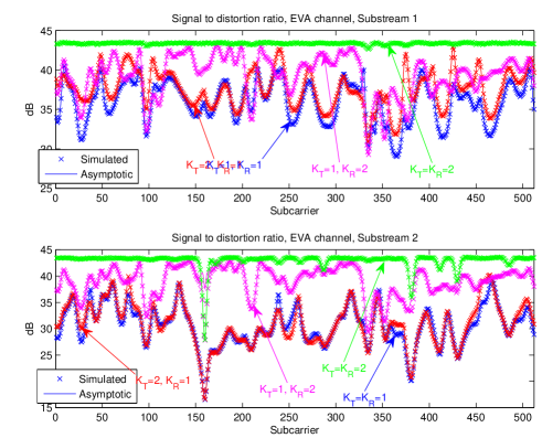
Figure 7: Signal to distortion power ratio measured at the output of the receiver when the transmitter uses SVD-type precoding and the receiver performs channel inversion. The simulated channel was the one represented in the upper plot of Fig. 6.

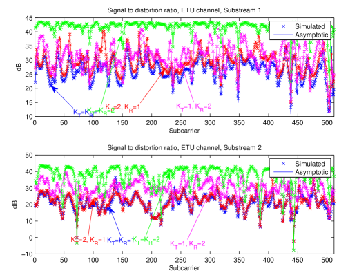
Figure 8: Signal to distortion power ratio measured at the output of the receiver when the transmitter uses SVD-type precoding and the receiver performs channel inversion. The simulated channel was the one represented in the lower plot of Fig. 6.

As for the actual performance of the multi-stage transceiver architecture, it is clearly seen that substantial gains can be achieved in terms of residual ICI/ISI reduction by simply implementing a second parallel stage at the transmitter/receiver. On the other hand, simulations confirm the fact that the performance is roughly dictated by the minimum number of parallel stages used at the transmit and receive sides, that is the minimum between $K_{R}$ and $K_{T}$. In other words, when using frequency-selective processing at both transmitter and receiver, the most important gains can be obtained by considering the proposed architecture at both sides of the communications link, but using the same number of parallel stages.

V-B Performance under general frequency-selective channels

In this subsection, we evaluate the performance under background noise and under a large set of randomly drawn channel frequency responses. The total number of subcarriers was set to $1024$ and the number of antennas was fixed to $N_{T}=2$ and $N_{R}=4$, and two different symbol streams were transmitted $N_{S}=2$. The transmitter was fixed to $\mathbf{A}(\omega)=\mathbf{I}_{N_{T}}$ (pure spatial multiplexing) whereas a LMMSE processor was considered at the receiver, i.e.

$$\mathbf{B}(\omega)=\mathbf{H}(\omega)\left(\mathbf{H}^{H}(\omega)\mathbf{H}(\omega)+\sigma^{2}/P_{S}\mathbf{I}_{N_{T}}\right)^{-1}.$$

Figs. 9 and 10 represent the cumulative distribution function of the measured mutual information per stream corresponding to $100$  realizations of EVA and ETU channel models respectively, for different values of the signal to noise power ratio. These mutual informations were estimated assuming Gaussian signaling and disregarding the statistical dependence between distortion and information symbols. Apart from the performance of the proposed receiver with multiple parallel stages, we also represent the performance of the multi-tap MIMO equalizer in [12], based on the frequency sampling technique, as well as the optimum performance under frequency flat equivalent channels. In the legend of the figures, we represent the percentage of increase of the corresponding technique in terms of real-valued multiplications (M%) and additions (A%) with respect to the traditional single tap per-subcarrier channel inversion (obtained as $K_{R}=1$). Observe that the parallel multi-stage architecture with $K_{R}=2$ presents a computational complexity that is comparable to a multi-tap processor with $N_{taps}=3$, but achieves a much better output SNDR, especially at low values of the background noise. In terms of the global SNDR distribution, two parallel stages are sufficient to provide a performance comparable to a multi-tap filter with $N_{taps}=7$ taps at a much lower computational complexity.

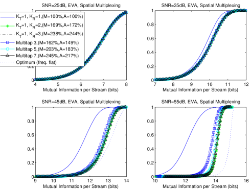
Figure 9: Mutual information distribution (bits per stream) for different levels of the background noise with $N_{T}=2$, $N_{R}=4$ and spatial multiplexing (EVA channel model).

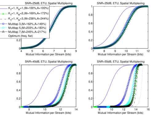
Figure 10: Mutual information distribution (bits per stream) for different levels of the background noise with $N_{T}=2$, $N_{R}=4$ and spatial multiplexing (ETU channel model).

Next, we considered a scenario with $N_{T}=4$ and $N_{R}=2$ where the precoder used the two left singular vectors associated with the largest singular values of the channel matrix. The linear filter at the receiver was fixed in order to invert the resulting channel matrix. Figs. 11 to 12 show the distribution of the estimated mutual information obtained with $100$ random realizations of the EVA and the ETU channel models respectively and for different values of the background noise power. Here again, we observe that high gains can be obtained with the proposed multi-stage MIMO architecture using only two stages at the transmitter and at the receiver.

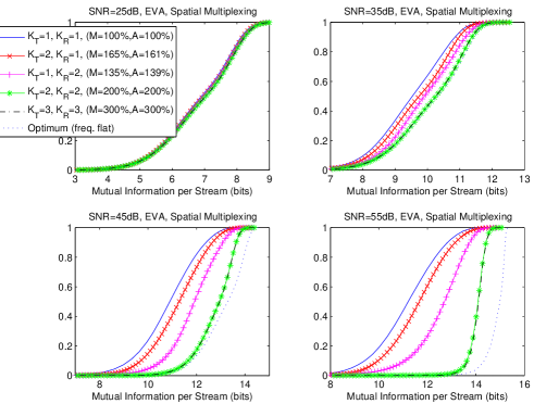
Figure 11: Mutual information distribution (bits per stream) for different levels of the background noise with $N_{T}=4$, $N_{R}=2$ and SVD-based precoding (EVA channel model).

Figure 12: Mutual information distribution (bits per stream) for different levels of the background noise with $N_{T}=4$, $N_{R}=2$ and SVD-based precoding (ETU channel model).

VI Conclusions

A novel parallel multi-stage MIMO architecture for FBMC transmissions under strong frequency selectivity has been presented. The rationale behind the approach consists in implementing a Taylor expansion of the ideal precoder and linear receiver at the central frequency of each subband. By properly exploiting the filterbank structure, it has been shown that the global system can be implemented using conventional per-subcarrier precoders/linear receivers in combination with parallel filterbanks constructed from sequential derivatives of an original prototype pulse. For the specific case of FBMC/OQAM, an asymptotic expression for the ICI/ISI distortion power has been obtained. It has been shown that the global performance of the system essentially depends on the minimum between the number of parallel stages implemented at the transmitter and the receiver. Finally, numerical evaluation studies indicate that the asymptotic performance assessment provides a very accurate approximation of the reality for moderate values of the number of subcarriers, and that significant gains can be obtained using the proposed architecture under strong frequency selectivity.

Appendix A Proof of Theorem 1

We begin the proof by introducing a technical result that will be used throughout this appendix, which will be separately proven.

Proposition 1

Let $\mathcal{Y}_{p,q}\left(\mathbf{S}_{n}\right)$ be the FBMC receive sample matrix corresponding to the symbol matrix $\mathbf{S}_{n}$ when the channel is ideal and the prototype pulses $p,q$ are used at the transmit/receive sides respectively. Let $F(\omega)$ denote a $\mathcal{C}^{R^{\prime}+1}\left(\mathbb{R}/2\pi\mathbb{Z}\right)$ function for some integer $R^{\prime}>\left(2R+1\right)\left(R+2\right)$, and let $\mathcal{Z}_{p,q}^{F}\left(\mathbf{S}_{n}\right)$ denote the matrix of received samples at the output of the decimators corresponding to $\mathcal{Y}_{p,q}\left(\mathbf{S}_{n}\right)$, when the signal goes through a channel with frequency response $F(\omega)$. Under $(\mathbf{As1})-(\mathbf{As3})$ for any integer $R>0$ we can write

$$\mathcal{Z}_{p,q}^{F}\left(\mathbf{S}_{n}\right) =\sum_{r=0}^{R}\frac{\left(-\textnormal{j}\right)^{r}}{r!\left(2M\right)^{r}}\Lambda\left(F^{\left(r\right)}\right)\mathcal{Y}_{p,q^{(r)}}\left(\mathbf{S}_{n}\right)+o\left(M^{-R}\right)$$ (22)

$$=\sum_{r=0}^{R}\frac{\left(-\textnormal{j}\right)^{r}}{r!\left(2M\right)^{r}}\mathcal{Y}_{p^{(r)},q}\left(\Lambda\left(F^{\left(r\right)}\right)\mathbf{S}_{n}\right)+o\left(M^{-R}\right)$$ (23)

where $F^{\left(r\right)}$ denotes the $r$th order derivative of the function $F$ and where $o\left(M^{-R}\right)\,$ for an integer $R$ denotes a matrix of potentially increasing dimensions whose entries decay to zero faster than $M^{-R}\,$ when $M\rightarrow\infty$. Furthermore, the above identities hold true also if either $p$ in (22) or $q$ in (23) are replaced by $p^{(k)}$ and $q^{(k)}$ for any integer $k\leq R$.

Proof:

The identity in (22) is proven in [19, Proposition 1] when $F\left(\omega\right)$ is the Fourier transform of a finite length sequence. The proof of the present result follows along the same lines, see further Appendix B. ∎

Corollary 1

Under the above conditions, let $G(\omega)$ denote another $\mathcal{C}^{R^{\prime}+1}\left(\mathbb{R}/2\pi\mathbb{Z}\right)$ function. Then,

$$\mathcal{Z}_{p,q}^{FG}\left(\mathbf{S}_{n}\right) =\sum_{k=0}^{R}\frac{\left(-\textnormal{j}\right)^{k}}{k!\left(2M\right)^{k}}\Lambda\left(G^{\left(k\right)}\right)\mathcal{Z}_{p,q^{(k)}}^{F}\left(\mathbf{S}_{n}\right)+o\left(M^{-R}\right)$$

$$=\sum_{k=0}^{R}\frac{\left(-\textnormal{j}\right)^{k}}{k!\left(2M\right)^{k}}\mathcal{Z}_{p^{(k)},q}^{F}\left(\Lambda\left(G^{\left(k\right)}\right)\mathbf{S}_{n}\right)+o\left(M^{-R}\right).$$

Furthermore, the above identities also hold when the zeroth order derivatives $p$ and $q$ are replaced by $p^{(k)}$ and $q^{(k)}$ for any integer $k\leq R$.

Proof:

We will only prove the first identity, the proof of second one being completely equivalent. Noting that $q^{(k)}\in\mathcal{C}^{R-k}$ and replacing $\mathcal{Z}_{p,q^{(k)}}^{F}\left(\mathbf{S}_{n}\right)$ by the corresponding expression in (22), with $R$ replaced by $R-k$ and $q$ replaced by $q^{(k)}$, we see that

$$\sum_{k=0}^{R}\frac{\left(-\textnormal{j}\right)^{k}}{k!\left(2M\right)^{k}}\Lambda\left(G^{\left(r\right)}\right)\mathcal{Z}_{p,q^{(k)}}^{F}\left(\mathbf{S}_{n}\right)$$

$$=\sum_{k=0}^{R}\sum_{r=0}^{R-k}\frac{\left(-\textnormal{j}\right)^{k+r}}{k!r!\left(2M\right)^{k+r}}\Lambda\left(G^{\left(r\right)}F^{\left(k\right)}\right)\mathcal{Y}_{p,q^{(k+r)}}\left(\mathbf{S}_{n}\right)$$

$$+o\left(M^{-R}\right)$$

$$\overset{\text{(a)}}{=}\sum_{m=0}^{R}\frac{\left(-\textnormal{j}\right)^{m}}{m!\left(2M\right)^{m}}\Lambda\left(\left(FG\right)^{(m)}\right)\mathcal{Y}_{p,q^{(m)}}\left(\mathbf{S}_{n}\right)+o\left(M^{-R}\right)$$

$$\overset{\text{(b)}}{=}\mathcal{Z}_{p,q}^{FG}\left(\mathbf{S}_{n}\right)+o\left(M^{-R}\right)$$

where in (a) we have replaced the index $r$ by the index $m=k+r$ and swapped the two sums and in (b) we have used again (22) with $F$ replaced by $FG$. ∎

This corollary will be very useful in order to characterize the asymptotic distortion error. Consider the expression of the received signal matrix $\mathcal{Z}_{n}$ in (10), which can be expressed as

$$\mathcal{Z}_{n} =\sum_{n_{{}_{S}},n_{T},n_{R}}\sum_{\ell_{2}=0}^{K_{R}-1}\frac{\left(-\textnormal{j}\right)^{\ell_{2}}}{\ell_{2}!\left(2M\right)^{\ell_{2}}}\Lambda\left(B_{n_{R},n}^{\left(\ell_{2}\right)\ast}\right)\times$$

$$\times\sum_{\ell_{1}=0}^{K_{T}-1}\frac{\left(-\textnormal{j}\right)^{\ell_{1}}}{\ell_{1}!\left(2M\right)^{\ell_{1}}}\mathcal{Z}_{p^{(\ell_{1})},q^{(\ell_{2})}}^{H_{n_{R},n_{T}}}\left(\Lambda\left(A_{n_{T},n_{{}_{S}}}^{\left(\ell_{1}\right)}\right)\mathbf{S}_{n_{S}}\right)$$

Applying Corollary 1 for $R=K_{T}+K_{R}$, we can write

$$\sum_{\ell_{1}=0}^{K_{T}-1}\frac{\left(-\textnormal{j}\right)^{\ell_{1}}}{\ell_{1}!\left(2M\right)^{\ell_{1}}}\mathcal{Z}_{p^{(\ell_{1})},q^{(\ell_{2})}}^{H_{n_{R},n_{T}}}\left(\Lambda\left(A_{n_{T},n_{{}_{S}}}^{\left(\ell_{1}\right)}\right)\mathbf{S}_{n_{S}}\right)$$

$$=\mathcal{Z}_{p,q^{(\ell_{2})}}^{H_{n_{R},n_{T}}A_{n_{T},n_{{}_{S}}}}\left(\mathbf{S}_{n}\right)$$

$$-\sum_{\ell_{1}=K_{T}}^{K_{T}+K_{R}}\frac{\left(-\textnormal{j}\right)^{\ell_{1}}}{\ell_{1}!\left(2M\right)^{\ell_{1}}}\mathcal{Z}_{p^{(\ell_{1})},q^{(\ell_{2})}}^{H_{n_{R},n_{T}}}\left(\Lambda\left(A_{n_{T},n_{{}_{S}}}^{\left(\ell_{1}\right)}\right)\mathbf{S}_{n_{S}}\right)$$

$$+o\left(M^{-\left(K_{T}+K_{R}\right)}\right)$$

and therefore inserting this into the expression of $\mathcal{Z}_{n}$ above and applying again Corollary 1 with respect to all the sums in the index $\ell_{2}$, we obtain

$$\mathcal{Z}_{n}=\sum_{n_{{}_{S}},n_{R},n_{T}}\left[\mathcal{Z}_{p,q}^{B_{n_{R},n}^{\ast}H_{n_{R},n_{T}}A_{n_{T},n_{{}_{S}}}}\left(\mathbf{S}_{n_{S}}\right)+\mathcal{E}_{n,n_{T},n_{R}}\left(\mathbf{S}_{n_{S}}\right)\right]$$

where

$$\mathcal{E}_{n,n_{T},n_{R}}\left(\mathbf{S}_{n_{S}}\right)$$

$$=-\sum_{\ell_{2}=K_{R}}^{K_{T}+K_{R}}\frac{\left(-\textnormal{j}\right)^{\ell_{2}}}{\ell_{2}!\left(2M\right)^{\ell_{2}}}\Lambda\left(B_{n_{R},n}^{\left(\ell_{2}\right)\ast}\right)\mathcal{Z}_{p,q^{(\ell_{2})}}^{H_{n_{R},n_{T}}A_{n_{T},n_{{}_{S}}}}\left(\mathbf{S}_{n_{S}}\right)$$

$$-\sum_{\ell_{1}=K_{T}}^{K_{T}+K_{R}}\frac{\left(-\textnormal{j}\right)^{\ell_{1}}}{\ell_{1}!\left(2M\right)^{\ell_{1}}}\mathcal{Z}_{p^{(\ell_{1})},q}^{B_{n_{R},n}^{\ast}H_{n_{R},n_{T}}}\left(\Lambda\left(A_{n_{T},n_{{}_{S}}}^{\left(\ell_{1}\right)}\right)\mathbf{S}_{n_{S}}\right)$$

$$+\frac{\left(-\textnormal{j}\right)^{K_{R}+K_{T}}}{K_{T}!K_{R}!\left(2M\right)^{K_{R}+K_{T}}}\Lambda\left(B_{n_{R},n}^{\left(K_{R}\right)\ast}\right)\times$$

$$\times\mathcal{Z}_{p^{(K_{T})},q^{(K_{R})}}^{H_{n_{R},n_{T}}}\left(\Lambda\left(A_{n_{T},n_{{}_{S}}}^{\left(K_{T}\right)}\right)\mathbf{S}_{n_{S}}\right)+o\left(M^{-\left(K_{T}+K_{R}\right)}\right).$$

Now, using the linearity of the transmission from different antennas and the fact that $\mathbf{B}^{H}(\omega)\mathbf{H}(\omega)\mathbf{A}(\omega)=\mathbf{I}_{N_{s}}$ we obtain

$$\mathcal{Z}_{n}=\mathcal{Y}_{p,q}\left(\mathbf{S}_{n}\right)+\sum_{n_{T}=1}^{N_{T}}\sum_{n_{R}=1}^{N_{R}}\sum_{n_{{}_{S}}=1}^{N_{S}}\mathcal{E}_{n,n_{T},n_{R}}\left(\mathbf{S}_{n_{S}}\right)$$

Using now Proposition 1 and disregarding all terms of higher order, we can readily see that (16) holds with

$$\mathcal{E}_{p,q}\left(\mathbf{S}_{n}\right)=\mathcal{E}_{p,q}^{(1)}\left(\mathbf{S}_{n}\right)+\mathcal{E}_{p,q}^{(2)}\left(\mathbf{S}_{n}\right)+\mathcal{E}_{p,q}^{(3)}\left(\mathbf{S}_{n}\right)+o\left(M^{-\left(K_{T}+K_{R}\right)}\right)$$ (24)

where we have introduced the matrices

$$\mathcal{E}_{p,q}^{(1)}\left(\mathbf{S}_{n}\right) =-\sum_{n_{{}_{S}}=1}^{N_{S}}\Upsilon_{n_{S}}$$ (25)

$$\mathcal{E}_{p,q}^{(2)}\left(\mathbf{S}_{n}\right) =-\sum_{n_{{}_{S}}=1}^{N_{S}}\sum_{m=K_{R}}^{K_{T}+K_{R}}\Lambda\left(\sum_{\ell_{2}=K_{R}}^{m}\beta_{n,n_{S}}^{(m,\ell)}\right)\frac{\mathcal{Y}_{p,q^{(m)}}\left(\mathbf{S}_{n_{{}_{S}}}\right)}{\sqrt{2}\left(2M\right)^{m}}$$ (26)

$$\mathcal{E}_{p,q}^{(3)}\left(\mathbf{S}_{n}\right) =\sum_{n_{{}_{S}}=1}^{N_{S}}\Lambda\left(\gamma_{n,n_{S}}\right)\frac{\mathcal{Y}_{p^{(K_{T})},q^{(K_{R})}}\left(\mathbf{S}_{n_{S}}\right)}{\sqrt{2}\left(2M\right)^{K_{R}+K_{T}}}$$ (27)

where $\beta_{n,n_{S}}^{(m,\ell)}$ and $\gamma_{n,n_{S}}$ are defined in (20) and (21) respectively, and where

$$\Upsilon_{n_{S}}=\sum_{m=K_{T}}^{K_{T}+K_{R}}\frac{\left(-\textnormal{j}\right)^{m}}{\left(2M\right)^{m}m!}\sum_{n_{T}=1}^{N_{T}}\sum_{\ell_{1}=K_{T}}^{m}\binom{m}{\ell_{1}}\times\\ \times\Lambda\left\{\left(\mathbf{B}^{H}\mathbf{H}\right)^{\left(m-\ell_{1}\right)}\right\}_{n,n_{T}}\mathcal{Y}_{p^{(\ell_{1})},q^{(m-\ell_{1})}}\left(\Lambda\left(A_{n_{T},n_{{}_{S}}}^{\left(\ell_{1}\right)}\right)\mathbf{S}_{n_{S}}\right).$$

Next, we transform $\Upsilon_{m,n_{S}}$ into a linear combination of matrices of the type $\mathcal{Y}_{p^{(i)},q^{(j)}}\left(\mathbf{S}_{n_{S}}\right)$ for some integers $i,j$. The following lemma will be instrumental in this objective.

Lemma 1

Under the assumptions of Proposition 1, we have

$$\mathcal{Y}_{p,q}\left(\Lambda\left(F\right)\mathbf{S}_{n}\right) =\sum_{m=0}^{R}\frac{\left(-\textnormal{j}\right)^{m}}{\left(2M\right)^{m}m!}\Lambda\left(F^{\left(m\right)}\right)\mathcal{Y}_{p,q}^{(m)}\left(\mathbf{S}_{n}\right)$$

$$+o\left(M^{-R}\right)$$

where we have defined

$$\mathcal{Y}_{p,q}^{(m)}\left(\mathbf{S}_{n}\right)=\sum_{r=0}^{m}\binom{m}{r}\left(-1\right)^{r}\mathcal{Y}_{p^{(r)},q^{(m-r)}}\left(\mathbf{S}_{n}\right).$$

Proof:

For $\ell=0,\ldots,R$, we consider the identities in (22)-(23) in Proposition 1 with $p$ and $F$ replaced by $p^{(\ell)}$ and $F^{(\ell)}$ respectively, that is

$$\sum_{r=0}^{R-\ell}\frac{\left(-\textnormal{j}\right)^{r+\ell}}{r!\left(2M\right)^{r+\ell}}\mathcal{Y}_{p^{(r+\ell)},q}\left(\Lambda\left(F^{\left(r+\ell\right)}\right)\mathbf{S}_{n}\right)$$

$$=\sum_{r=0}^{R-\ell}\frac{\left(-\textnormal{j}\right)^{r+\ell}}{r!\left(2M\right)^{r+\ell}}\Lambda\left(F^{\left(r+\ell\right)}\right)\mathcal{Y}_{p^{(\ell)},q^{(r)}}\left(\mathbf{S}_{n}\right)+o\left(M^{-R}\right).$$

This forms a system of $R+1$ linear equations with $R+1$ unknowns, which can be expressed in matrix form as

$$\mathbb{A}_{R}\mathbf{x}_{R}=\mathbf{y}_{R}+o\left(M^{-R}\right)$$

where $\mathbf{x}_{R}=\left[x_{0},\ldots,x_{R}\right]^{T}$, $\mathbf{y}_{R}=\left[y_{0},\ldots,y_{R}\right]^{T}$,

$$x_{r} =\frac{\left(-\textnormal{j}\right)^{r}}{\left(2M\right)^{r}}\mathcal{Y}_{p^{(r)},q}\left(\Lambda\left(F^{\left(r\right)}\right)\mathbf{S}_{n}\right)$$

$$y_{r} =\sum_{m=0}^{R-r}\frac{\left(-\textnormal{j}\right)^{m+r}}{m!\left(2M\right)^{m+r}}\Lambda\left(F^{\left(m+r\right)}\right)\mathcal{Y}_{p^{(r)},q^{(m)}}\left(\mathbf{S}_{n}\right)$$ (28)

and where $\mathbb{A}_{R}$ is an $R\times R$ upper triangular Toeplitz matrix with the entries of the $m$th upper diagonal fixed to $1/m$!, $m=0,\ldots,R$. We are interested in obtaining the solution associated with the first entry of $\mathbf{x}_{R}$, so that we will be able to write

$$x_{0}=\mathcal{Y}_{p,q}\left(\Lambda\left(F\right)\mathbf{S}_{n}\right)=\sum_{j=0}^{R}\xi_{j}y_{j}+o\left(M^{-R}\right)$$ (29)

where $\xi_{j}$ are the entries of the upper row of $\mathbb{A}_{R}^{-1}$. We can iteratively obtain the solution to $\xi_{j}$ by observing that we can partition this matrix as

$$\mathbb{A}_{R}=\left[\begin{array}[c]{cc}\mathbb{A}_{R-1}&\mathbf{J}_{R-1}\mathbf{a}_{R}\\ 0&1\end{array}\right]$$

where $\mathbf{a}_{R}=\left[a_{1},\ldots,a_{R}\right]^{T}$, so that

$$\mathbb{A}_{R}^{-1}=\left[\begin{array}[c]{cc}\mathbb{A}_{R-1}^{-1}&-\mathbb{A}_{R-1}^{-1}\mathbf{J}_{R-1}\mathbf{a}_{R}\\ 0&1\end{array}\right]$$

and this basically implies that $\xi_{0}=1$ and

$$\xi_{R}=-\sum_{m=0}^{R-1}\xi_{m}a_{R-m}=-\sum_{m=0}^{R-1}\frac{1}{(R-m)!}\xi_{m}.$$

We can solve this recurrence by noting that it can be rewritten as

$$R!\xi_{R}=-\sum_{m=0}^{R-1}\binom{R}{m}m!\xi_{m}$$

which basically implies that $m!\xi_{m}=\left(-1\right)^{m}$. Using this together with the expression of $y_{r}$ in (28) and swapping the two indexes we obtain the result of the lemma.∎

Applying Lemma 1 we can rewrite $\Upsilon_{n_{S}}$ as

$$\Upsilon_{n_{S}}=\sum_{m=K_{T}}^{K_{T}+K_{R}}\frac{\left(-\textnormal{j}\right)^{m}}{m!\left(2M\right)^{m}}\sum_{k=K_{T}}^{m}\sum_{\ell_{1}=K_{T}}^{k}\binom{m}{k}\binom{k}{\ell_{1}}\times\\ \times\Lambda\left(\left\{\left(\mathbf{B}^{H}\mathbf{H}\right)^{\left(k-\ell_{1}\right)}\mathbf{A}^{\left(\ell_{1}+m-k\right)}\right\}_{n,n_{S}}\right)\mathcal{Y}_{p^{(\ell_{1})},q^{(k-\ell_{1})}}^{(m-k)}\left(\mathbf{S}_{n_{S}}\right)\\ +o\left(M^{-\left(K_{T}+K_{R}\right)}\right)$$

Using the fact that

$$\binom{m}{k}\binom{k}{\ell_{1}}=\binom{m}{k-\ell_{1}}\binom{m-k+\ell_{1}}{\ell_{1}}$$ (30)

and with the appropriate change of indexes ($\ell=m-k+\ell_{1}$), we see that

$$\Upsilon_{n_{S}}=\sum_{m=K_{T}}^{K_{T}+K_{R}}\frac{1}{\sqrt{2}\left(2M\right)^{m}}\Lambda\left(\sum_{\ell=K_{T}}^{m}\alpha_{n,n_{S}}^{(m,\ell)}\right)\times\\ \times\sum_{k=K_{T}+m-\ell}^{m}\binom{\ell}{m-k}\mathcal{Y}_{p^{(k-(m-\ell))},q^{(m-\ell)}}^{(m-k)}\left(\mathbf{S}_{n_{S}}\right)+o\left(M^{-\left(K_{T}+K_{R}\right)}\right)$$

where $\alpha_{n,n_{S}}^{(m,\ell)}$ is defined in (19). Finally, using the change of indexes ($j=k-m+\ell+r$) together with (30), the additional change of indexes $s=\left(j+m-\ell\right)-k$ and the identity

$$\sum_{s=0}^{j-K_{T}}\left(-1\right)^{s}\binom{j}{s}=\left(-1\right)^{j-K_{T}}\binom{j-1}{j-K_{T}}$$

we finally obtain

$$\Upsilon_{n_{S}}=\sum_{m=K_{T}}^{K_{T}+K_{R}}\frac{1}{\sqrt{2}\left(2M\right)^{m}}\Lambda\left(\sum_{\ell=K_{T}}^{m}\alpha_{n,n_{S}}^{(m,\ell)}\right)\times\\ \times\sum_{j=K_{T}}^{\ell}\left(-1\right)^{j+K_{T}}\binom{\ell}{j}\binom{j-1}{K_{T}-1}\mathcal{Y}_{p^{(j)},q^{(m-j)}}\left(\mathbf{S}_{n_{S}}\right)\\ +o\left(M^{-\left(K_{T}+K_{R}\right)}\right)$$

Inserting this into the expression of $\mathcal{E}_{p,q}^{(1)}\left(\mathbf{S}_{n}\right)$ in (25), we end up with an expression of $\mathcal{E}_{p,q}\left(\mathbf{S}_{n}\right)$ in (24) that is a linear combination of matrices of the form $\mathcal{Y}_{p^{(m)},q^{(n)}}\left(\mathbf{S}_{n_{S}}\right)$ for different integers $m,n$. Therefore, we can analyze the asymptotic distortion variance by simply analyzing these terms. We provide more details in what follows.

From the definition of the complex estimated symbols $\mathbf{\hat{s}}_{n}\left(\ell\right)$ in (17), we see that this column vector is a function of two columns of the matrix $\mathcal{Z}_{p,q}\left(\mathbf{S}_{n}\right)$, namely

$$\mathbf{z}_{n,\ell}^{\text{odd}}\left(p,q\right)\overset{\textnormal{def}}{=}\left[\mathcal{Z}_{p,q}^{\text{odd}}\left(\mathbf{S}_{n}\right)\right]_{:,\ell+\kappa-1}\text{ }$$

$$\mathbf{z}_{n,\ell}^{\text{even}}\left(p,q\right)\overset{\textnormal{def}}{=}\left[\mathcal{Z}_{p,q}^{\text{even}}\left(\mathbf{S}_{n}\right)\right]_{:,\ell+\kappa}.$$

Let us equivalently define $\mathbf{y}_{n,\ell}^{\text{odd}}\left(p,q\right)$ and $\mathbf{y}_{n,\ell}^{\text{even}}\left(p,q\right)$ as above, replacing $\mathcal{Z}$ by $\mathcal{Y}$. We define the error associated to the estimation of the $\ell$th multicarrier symbol of the $n$th stream as $\mathbf{e}_{n,\ell}\left(p,q\right)=\mathbf{\hat{s}}_{n}\left(\ell\right)-\mathbf{s}_{n}\left(\ell\right)$, so that

$$\mathbf{e}_{n,\ell}\left(p,q\right)=\textnormal{Re}\left[\mathbf{z}_{n,\ell}^{\text{odd}}\left(p,q\right)\right]+\textnormal{j}\textnormal{Im}\left[\mathbf{z}_{n,\ell}^{\text{even}}\left(p,q\right)\right]-\mathbf{s}_{n}\left(\ell\right)$$

Now, from the asymptotic description provided above we have been able to express $\mathcal{Z}_{n}\left(p,q\right)$ as a function of matrices of the form $\mathcal{Y}_{p^{(m)},q^{(k)}}\left(\mathbf{S}_{n}\right)$ when $M\rightarrow\infty$ for several pairs of integers $m,k$. Consequently, $\mathbf{\hat{s}}_{n}\left(\ell\right)$ is asymptotically described as a weighted linear combination of $\mathbf{y}_{n,\ell}^{\text{odd}}\left(p^{(m)},q^{(k)}\right)$ and $\mathbf{y}_{n,\ell}^{\text{even}}\left(p^{(m)},q^{(k)}\right)\,$ for several pairs of integers $m,k$. In order to analyze the structure of $\mathcal{Y}_{n}$, let $\mathbf{F}$ denote the $2M\times 2M$ orthogonal Fourier matrix, and let $\mathbf{F}_{1}$ and $\mathbf{F}_{2}$ be the matrices formed by selecting the $M$ upper and lower rows of $\mathbf{F}$ respectively. The expression of $\mathcal{Y}_{n}^{\text{odd}}$ for FBMC/OQAM modulations can be shown to be [19]

$$\mathcal{Y}_{p,q}^{\text{odd}}\left(\mathbf{S}_{n}\right)=2\mathbf{\Phi F}^{H}\left(\left[\mathbf{F\Phi}^{\ast}\mathbf{B}_{n}\mathbf{,0,0}\right]\circledast\mathcal{R}\left(p,q\right)\right)\\ +2\mathbf{\Phi F}^{H}\left(\left[\begin{array}[c]{c}\mathbf{0},\mathbf{F}_{2}\mathbf{\Phi}^{\ast}\textnormal{j}\mathbf{C}_{n}\mathbf{,0}\\ \mathbf{F}_{1}\mathbf{\Phi}^{\ast}\textnormal{j}\mathbf{C}_{n}\mathbf{,0,0}\end{array}\right]\circledast\mathcal{S}\left(p,q\right)\right)$$ (31)

where $\mathcal{R}\left(p,q\right)$, $\mathcal{S}\left(p,q\right)$ are defined in (13)-(14), $\mathbf{\Phi}$ is a diagonal matrix with its $m$th diagonal entry equal to $\exp\left(-\textnormal{j}\pi\frac{M+1}{M}\left(m-1\right)\right)$ and $\mathbf{0}$ is an all-zeros column vector of appropriate dimensions. A similar expression can be given for $\mathcal{Y}_{n}^{\text{even}}$, see further [19, eq. (4)].

Now, recalling that $\mathcal{I}$ is a $2M\times\left(2\kappa-1\right)$ matrix with ones in the central column and zeros elsewhere, we observe that we are able to write

$$\mathbf{b}_{n}\left(\ell\right)=\left\{2\mathbf{\Phi F}^{H}\left(\left[\mathbf{F\Phi}^{\ast}\mathbf{B}_{n}\mathbf{,0,0}\right]\circledast\frac{1}{2}\mathcal{I}\right)\right\}_{:,\ell+\kappa-1}$$ (32)

and this identity holds true if we replace the pair $\mathbf{b}_{n}\left(\ell\right)$, $\mathbf{B}_{n}$ by $\mathbf{c}_{n}\left(\ell\right)$, $\mathbf{C}_{n}$. Using (32) and replacing $\mathbf{z}_{n,\ell}^{\text{odd}}\left(p,q\right)$ by the asymptotic expansion, we see that

$$\mathbf{z}_{n,\ell}^{\text{odd}}\left(p,q\right)-\mathbf{b}_{n}\left(\ell\right)$$

$$=\mathbf{d}_{n,\ell}^{\text{odd}}\left(p,q\right)$$

$$-\sum_{n_{{}_{S}}=1}^{N_{S}}\sum_{m=K_{T}}^{K_{T}+K_{R}}\frac{1}{\sqrt{2}\left(2M\right)^{m}}\sum_{\ell=K_{T}}^{m}\Lambda\left(\alpha_{n,n_{S}}^{(m,\ell)}\right)\times$$

$$\times\sum_{j=K_{T}}^{\ell}\left(-1\right)^{j-K_{T}}\binom{\ell}{j}\binom{j-1}{K_{T}-1}\mathbf{y}_{n_{S},\ell}^{\text{odd}}\left(p^{(j)},q^{(m-j)}\right)$$

$$-\sum_{n_{{}_{S}}=1}^{N_{S}}\sum_{m=K_{R}}^{K_{T}+K_{R}}\frac{1}{\sqrt{2}\left(2M\right)^{m}}\Lambda\left(\beta_{n,n_{S}}^{(m)}\right)\mathbf{y}_{n_{S},\ell}^{\text{odd}}\left(p,q^{(m)}\right)$$

$$+\frac{1}{\sqrt{2}\left(2M\right)^{K_{R}+K_{T}}}\sum_{n_{{}_{S}}=1}^{N_{S}}\Lambda\left(\gamma_{n,n_{S}}\right)\mathbf{y}_{n_{S},\ell}^{\text{odd}}\left(p^{(K_{T})},q^{(K_{R})}\right)$$

$$+o\left(M^{-\left(K_{T}+K_{T}\right)}\right)$$

where $\mathbf{d}_{n,\ell}^{(\ast)}\left(p,q\right)$, $(\ast)\in\left\{\text{odd,even}\right\}$, is defined as $\mathbf{y}_{n,\ell}^{(\ast)}\left(p,q\right)$ by simply replacing $\mathcal{R}\left(p,q\right)$ with $\mathcal{R}\left(p,q\right)-\frac{1}{2}\mathcal{I}$ in (31). An equivalent expression can be derived for $\mathbf{z}_{n,\ell}^{\text{even}}\left(p,q\right)-\textnormal{j}\mathbf{c}_{n}\left(\ell\right)$, which is omitted here due to space constraints. The expressions presented in Theorem 1 are obtained by computing the variance of $\left\{\mathbf{e}_{n,\ell}\left(p,q\right)\right\}_{k}$ and disregarding the higher order terms. This can be easily done using the following result, which can be proven as in [19, Appendix B].

Lemma 2

Consider now four generic prototype filters $p_{1},q_{1},p_{2},q_{2}$, and denote $\mathcal{R}_{i}=\mathcal{R}\left(p_{i},q_{i}\right)$ and $\mathcal{S}_{i}=\mathcal{S}\left(p_{i},q_{i}\right)$, $i=1,2$. Write for compactness $\mathbf{\bar{y}}_{n,\ell,i}^{(\ast)}=\mathbf{\bar{y}}_{n,\ell}^{(\ast)}\left(p_{i},q_{i}\right)\,$,$\ i=1,2$, $(\ast)\in\left\{\text{even,odd}\right\}$ and let $\ell\in\left\{\kappa,\ldots,N-\kappa\right\}$. Under $\mathbf{(As4)}$, and for the FBMC/OQAM signal model we can write

$$\mathbb{E}\left[\textnormal{Re}\left\{\mathbf{y}_{n,\ell,1}^{\text{odd}}\right\}_{k}\textnormal{Re}\left\{\mathbf{y}_{n,\ell,2}^{\text{odd}}\right\}_{k}\right] =\mathbb{E}\left[\textnormal{Im}\left\{\mathbf{y}_{n,\ell,1}^{\text{even}}\right\}_{k}\textnormal{Im}\left\{\mathbf{y}_{n,\ell,2}^{\text{even}}\right\}_{k}\right]$$

$$=\eta^{\left(+,-\right)}\left(\mathcal{R}_{1}\mathcal{R}_{2}^{T},\mathcal{S}_{1}\mathcal{S}_{2}^{T}\right)$$

$$\mathbb{E}\left[\textnormal{Im}\left\{\mathbf{y}_{n,\ell,1}^{\text{odd}}\right\}_{k}\textnormal{Im}\left\{\mathbf{y}_{n,\ell,2}^{\text{odd}}\right\}_{k}\right] =\mathbb{E}\left[\textnormal{Re}\left\{\mathbf{y}_{n,\ell,1}^{\text{even}}\right\}_{k}\textnormal{Re}\left\{\mathbf{y}_{n,\ell,2}^{\text{even}}\right\}_{k}\right]$$

$$=\eta^{\left(-,+\right)}\left(\mathcal{R}_{1}\mathcal{R}_{2}^{T},\mathcal{S}_{1}\mathcal{S}_{2}^{T}\right)$$

$$\mathbb{E}\left[\textnormal{Re}\left\{\mathbf{y}_{n,\ell,1}^{\text{odd}}\right\}_{k}\textnormal{Im}\left\{\mathbf{y}_{n,\ell,2}^{\text{odd}}\right\}_{k}\right] =\mathbb{E}\left[\textnormal{Re}\left\{\mathbf{y}_{n,\ell,1}^{\text{even}}\right\}_{k}\textnormal{Im}\left\{\mathbf{y}_{n,\ell,2}^{\text{even}}\right\}_{k}\right]$$

$$=0$$

where we have defined for $s_{1},s_{2}\in\left\{+,-\right\}$,

$$\eta^{\left(s_{1},s_{2}\right)}\left(\mathcal{R}_{1}\mathcal{R}_{2}^{T},\mathcal{S}_{1}\mathcal{S}_{2}^{T}\right)=\frac{P_{s}}{2M}\textnormal{tr}\left[\mathcal{R}_{1}\mathcal{R}_{2}^{T}\mathbf{U}^{s_{1}}+\mathcal{S}_{1}\mathcal{S}_{2}^{T}\mathbf{U}^{s_{2}}\right].$$

Furthermore, if $\mathbf{y}_{n,\ell,i}^{(\ast)}$ is replaced by $\mathbf{d}_{n,\ell,i}^{(\ast)}=\mathbf{d}_{n,\ell}^{(\ast)}\left(p_{i},q_{i}\right)$ in any of the above expressions, the same results hold replacing $\mathcal{R}_{i}$ by $\mathcal{R}_{i}-\frac{1}{2}\mathcal{I}$.

Appendix B Proof of Proposition 1

Let $\mathcal{Z}_{n}^{F}\left(p,q\right)$ denote the $2M\times 2\left(N+2\kappa\right)$ matrix containing the received samples at the output of the receive FFT corresponding to the $n$th transmit stream, assuming that the transmit and receive prototype pulses are $p$ and $q$ respectively. For the rest of the proof, we will drop the dependence on $n\,\$in that matrix, and we will decompose $\mathcal{Z}^{F}\left(p,q\right)=\mathcal{Z}_{\text{even}}^{F}\left(p,q\right)\otimes\left[1,0\right]+\mathcal{Z}_{\text{odd}}^{F}\left(p,q\right)\otimes\left[0,1\right]\,$. We will denote by $f\left[\ell\right]$ the $\ell$th coefficient of the Fourier series of $F(\omega)$, i.e.

$$f\left[\ell\right]=\frac{1}{2\pi}\int_{0}^{2\pi}F\left(\omega\right)\textnormal{e}^{\textnormal{j}\omega\ell}d\omega.$$

Furthermore, in order to describe the effect of the frequency selectivity of $F\left(\omega\right)$, we introduce the following pulse-specific matrices, defined for any $\ell\in\mathbb{Z}$ such that $-M<\ell\leq M$,

$$\mathcal{R}_{\ell}\left(p,q\right) =\mathbf{P\circledast J}_{2M}\mathbf{Q}(\ell)=\left[\begin{array}[c]{c}\mathbf{P}_{1}\circledast\mathbf{J}_{M}\mathbf{Q}_{2}(\ell)\\ \mathbf{P}_{2}\circledast\mathbf{J}_{M}\mathbf{Q}_{1}(\ell)\end{array}\right]$$

$$\mathcal{S}_{\ell}\left(p,q\right) =\left[\begin{array}[c]{c}\mathbf{0},\mathbf{P}_{2}\circledast\mathbf{J}_{M}\mathbf{Q}_{2}(\ell)\\ \mathbf{P}_{1}\circledast\mathbf{J}_{M}\mathbf{Q}_{1}(\ell)\mathbf{,0}\end{array}\right]\text{ }$$

where $\mathbf{Q}(\ell)$ is defined as

$$\mathbf{Q}(\ell) =\left[\begin{array}[c]{c}\mathbf{0},\mathbf{0},\left\{\mathbf{Q}\right\}_{2M-\ell+1:2M,:}\\ \mathbf{0},\left\{\mathbf{Q}\right\}_{1:2M-\ell,:},\mathbf{0}\end{array}\right],\text{ }0\leq\ell\leq M,$$

$$\mathbf{Q}(\ell) =\left[\begin{array}[c]{c}\mathbf{0},\left\{\mathbf{Q}\right\}_{-\ell+1:2M,:},\mathbf{0}\\ \left\{\mathbf{Q}\right\}_{1:-\ell,:},\mathbf{0,0}\end{array}\right],\text{ }-M<\ell<0\text{ }$$

so that $\mathbf{Q}(0)=[\mathbf{0},\mathbf{Q]}$. Furthermore, given a column vector of $2M$ entries $\mathbf{u}$, we define $\mathcal{M}(\mathbf{u})$ as the $2M\times 2M$ matrix

$$\mathcal{M}(\mathbf{u})=\Phi\mathbf{F}^{H}\textnormal{diag}\left(\mathbf{F}\Phi^{\ast}\mathbf{u}\right)$$

where $\mathbf{F}$ is the $2M$ Fourier matrix, $\left\{\mathbf{F}\right\}_{ij}=\left(2M\right)^{-1/2}\textnormal{e}^{\textnormal{j}2\pi\left(i-1\right)\left(j-1\right)/\left(2M\right)}$, $1\leq i,j\leq 2M$, and where $\Phi$ is a $2M\times 2M$ diagonal matrix with entries $\left\{\Phi\right\}_{kk}=\textnormal{e}^{-\textnormal{j}\pi\left(M+1\right)\left(k-1\right)/\left(2M\right)}$, $k=1,\ldots,2M$.

We will provide here the proof of (22), the proof of (23) following the same line of reasoning. Furthermore, we will only show that (22) holds for the odd columns of $\mathcal{Z}^{F}\left(p,q\right)$, namely $\mathcal{Z}_{\text{odd}}^{F}\left(p,q\right)$, since the proof for $\mathcal{Z}_{\text{even}}^{F}\left(p,q\right)$ is almost identical. Using the above definitions and following [19, eq. (14)-(15)], we can write

$$\left\{\mathcal{Z}_{\text{odd}}^{F}\left(p,q\right)\right\}_{:,i}=\\ =2\sum_{\ell=-\infty}^{\infty}\sum_{j=1}^{N}f\left[\ell\right]\Theta^{\ell}\Bigg{[}\mathcal{M}(\mathbf{b}_{j})\left\{\mathcal{R}_{\left\langle\ell\right\rangle_{2M}}\left(p,q\right)\right\}_{:,i-j-\left[\ell\right]_{2M}+2}\\ +\mathcal{M}(\textnormal{j}\mathbf{c}_{j})\left\{\mathcal{S}_{\left\langle\ell\right\rangle_{2M}}\left(p,q\right)\right\}_{:,i-j-\left[\ell\right]_{2M}+2}\Bigg{]}$$

where $\Theta$ is a diagonal matrix with entries $\left\{\Theta\right\}_{kk}=\textnormal{e}^{-\textnormal{j}\omega_{k}}$, $k=1,\ldots,2M$, $\left[\ell\right]_{2M}\$returns the integer that is closest to $\ell/(2M)$ (with the convention that  $[\left(2m+1\right)M]_{2M}=m$ when $m\in\mathbb{Z}$) and where $\left\langle\ell\right\rangle_{2M}=\ell-[\ell]_{2M}$. Now, following the approach in [19], we see that we can write

$$\left\{\mathcal{Z}_{\text{odd}}^{F}\left(p,q\right)-\sum_{r=0}^{R}\frac{\left(-\textnormal{j}\right)^{r}}{r!\left(2M\right)^{r}}\Lambda\left(F^{\left(r\right)}\right)\mathcal{Y}_{\text{odd}}\left(p,q^{(r)}\right)\right\}_{:,i}$$

$$=2\sum_{\ell=-\infty}^{\infty}\sum_{j=1}^{N}f\left[\ell\right]\Theta^{\ell}\Bigg{[}\mathcal{M}(\mathbf{b}_{j})\left\{\mathcal{E}_{\left\langle\ell\right\rangle_{2M},R}^{1}\right\}_{:,i-j-\left[\ell\right]_{2M}+2}$$

$$+\mathcal{M}(\textnormal{j}\mathbf{c}_{j})\left\{\mathcal{E}_{\left\langle\ell\right\rangle_{2M},R}^{2}\right\}_{:,i-j-\left[\ell\right]_{2M}+2}\Bigg{]}$$ (33)

where we have defined, for $-M<\ell\leq M,$

$$\mathcal{E}_{\ell,R}^{1} =\mathcal{R}_{\ell}\left(p,q\right)-\sum_{t=0}^{R}\frac{\left(-\ell\right)^{t}}{t!\left(2M\right)^{t}}\mathcal{R}_{0}\left(p,q^{(t)}\right)$$

$$\mathcal{E}_{\ell,R}^{2} =\mathcal{S}_{\ell}\left(p,q\right)-\sum_{t=0}^{R}\frac{\left(-\ell\right)^{t}}{t!\left(2M\right)^{t}}\mathcal{S}_{0}\left(p,q^{(t)}\right)$$

and where we have used the fact that (using the integration by parts formula)

$$\frac{1}{2\pi}\int_{0}^{2\pi}F^{t}\left(\omega\right)\textnormal{e}^{\textnormal{j}\omega\ell}d\omega=\ell^{t}\left(-\textnormal{j}\right)^{t}f\left[\ell\right],\ 0\leq t\leq R.$$

Now, we separate the global sum in (33) into two terms, which will be bounded in a different way. Consider a parameter $\delta\in\left(0,1\right)$ and divide the sum with respect to $\ell$ in (33) in two terms, corresponding to $\left|\ell\right|<M^{\delta}$ and $\left|\ell\right|\geq M^{\delta}$. Let us denote by $\chi_{1}$ and $\chi_{2}$ these two terms, so that $(\ref{eq:comberrorpulse})=\chi_{1}+\chi_{2}$, where $\chi_{1}=\sum_{\left|\ell\right|\geq M^{\delta}}($·$)$ and $\chi_{2}=\sum_{\left|\ell\right|<M^{\delta}}($·$)$. These two terms will be bounded using different methods, as it is described next.

B-A Bounding the term $\chi_{1}$

First observe that we can bound the $\left(m,n\right)$th entry of $\mathcal{E}_{\ell,R}^{1}$ as

$$\left|\left\{\mathcal{E}_{\ell,R}^{1}\right\}_{m,n}\right| \leq\left|\left\{\mathcal{R}_{\ell}\left(p,q\right)\right\}_{m,n}\right|$$

$$+\sum_{t=0}^{R}\frac{1}{t!}\left|\frac{\ell}{2M}\right|^{t}\left|\left\{\mathcal{R}_{0}\left(p,q^{(t)}\right)\right\}_{m,n}\right|.$$

Now, since the two pulses $p,q$ and their derivatives are bounded by assumption, the absolute value of the entries of $\mathcal{R}_{\ell}\left(p,q\right)$ and $\mathcal{R}_{0}\left(p,q^{(t)}\right)$ are upper bounded by a positive constant independent of $M$, denoted here by$\ C$. Therefore, since $\left|\ell\right|<M$ in the definition of $\mathcal{E}_{\ell,R}^{1}$,

$$\left|\left\{\mathcal{E}_{\ell,R}^{1}\right\}_{m,n}\right|\leq C+C\sum_{t=0}^{R}\frac{1}{t!}\left|\frac{\ell}{2M}\right|^{t}\leq C\left(1+\sum_{t=0}^{R}\frac{2^{-t}}{t!}\right)$$

which is bounded by a positive constant independent of $M$. A similar reasoning can be applied to show that $\left|\left\{\mathcal{E}_{\ell,R}^{2}\right\}_{i,j}\right|$ has the same property. Therefore, we see that (using the triangular and the Cauchy-Schwarz inequality),

$$\left|\left\{\chi_{1}\right\}_{k,i}\right|\leq 2\sum_{\left|\ell\right|\geq M^{\delta}}\left|f\left[\ell\right]\right|\\ \sum_{j=1}^{N}\Bigg{[}\left\|\left\{\mathcal{M}(\mathbf{b}_{j})\right\}_{k,:}\right\|\left\|\left[\mathcal{E}_{\textnormal{smod}\left(\ell,M\right),R}^{1}\right]_{:,i-j+\left[\ell/(2M)\right]+2}\right\|+\\ +\left\|\left\{\mathcal{M}(\textnormal{j}\mathbf{c}_{j})\right\}_{k,:}\right\|\left\|\left[\mathcal{E}_{\textnormal{smod}\left(\ell,M\right),R}^{2}\right]_{:,i-j+\left[\ell/(2M)\right]+2}\right\|\Bigg{]}\\ \leq K_{1}\sqrt{M}\left(\left\|\left\{\mathcal{M}(\mathbf{b}_{j})\right\}_{k,:}\right\|+\left\|\left\{\mathcal{M}(\textnormal{j}\mathbf{c}_{j})\right\}_{k,:}\right\|\right)\sum_{\left|\ell\right|\geq M^{\delta}}\left|f\left[\ell\right]\right|\\ \leq K_{2}\sqrt{M}\sum_{\left|\ell\right|\geq M^{\delta}}\left|f\left[\ell\right]\right|$$

for some positive constants $K_{1},K_{2}$ independent of $M$, where in the last equation we have used the fact that $\left\|\left\{\mathcal{M}(\mathbf{u})\right\}_{k,:}\right\|$ is bounded above if the entries of $\mathbf{u}$ are bounded (see further [19, p.3604]). Finally, we need the following result:

Lemma 3

If $F\in\mathcal{C}^{R^{\prime}+1}\left(\mathbb{R}/2\pi\mathbb{Z}\right)$, the $k$th Fourier coefficient $f[k]$ can be bounded by

$$\left|f[k]\right|\leq\frac{c}{\left|k\right|^{R^{\prime}+1}}$$

for some positive constant $c$.

Proof:

Applying the partial integration formula to the definition $f\left[k\right]$ consecutively $R^{\prime}+1$ times,

$$f\left[k\right]=\frac{\left(-1\right)^{R^{\prime}+1}}{2\pi\left(\textnormal{j}k\right)^{R^{\prime}+1}}\int_{0}^{2\pi}F^{\left(R^{\prime}+1\right)}\left(\omega\right)\textnormal{e}^{\textnormal{j}\omega k}d\omega$$

and therefore the result follows by the triangular inequality for integrals, taking $c=\sup_{\omega\in\mathbb{R}/2\pi\mathbb{Z}}\left|F^{R^{\prime}+1}\left(\omega\right)\right|$.∎

Applying this lemma, we readily see that there exists some positive constant $K\,\$such that, for any $\epsilon>0$,

$$\left|\left\{\chi_{1}\right\}_{k,i}\right|\leq K\sqrt{M}\sum_{\ell\geq M^{\delta}}\frac{1}{\ell^{R^{\prime}+1}}\leq\\ \leq\frac{K}{M^{\delta\left(R^{\prime}-\epsilon\right)-1/2}}\sum_{\ell\geq M^{\delta}}\frac{1}{\ell^{1+\epsilon}}=O\left(M^{-\delta\left(R^{\prime}-\epsilon\right)+1/2}\right).$$

B-B Bounding the term $\chi_{2}$

In order to analyze this term, we will use the following result, which can be proven as in [19, Lemma 1].

Lemma 4

Let $\ell\in\mathbb{Z}$ be such that $\left|\ell\right|<M$. Then, under $\mathbf{(As1)}$,

$$\left|\left\{\mathcal{E}_{\ell,R}^{1}\right\}_{m,n}\right|\leq K\left|\frac{\ell}{M}\right|^{R+1}\text{, }\left|\left\{\mathcal{E}_{\ell,R}^{2}\right\}_{m,n}\right|\leq K\left|\frac{\ell}{M}\right|^{R+1}$$

for some positive constant $K$, independent of $M,m,n$ and $\ell$.

Using this, we readily see that, by the Cauchy-Schwarz inequality,

$$\left|\left\{\chi_{2}\right\}_{k,i}\right|\leq 2\sum_{\left|\ell\right|<M^{\delta}}\left|f\left[\ell\right]\right|\times\\ \sum_{j=1}^{N}\left|\left\{\mathcal{M}(\mathbf{b}_{j})\right\}_{k,:}\left[\mathcal{E}_{\ell,R}^{1}\right]_{:,i-j+2}\right|+\left|\left\{\mathcal{M}(\textnormal{j}\mathbf{c}_{j})\right\}_{k,:}\left[\mathcal{E}_{\ell,R}^{2}\right]_{:,i-j+2}\right|\\ \leq K\sqrt{M}\sum_{\left|\ell\right|<M^{\delta}}\left|f\left[\ell\right]\right|\left|\frac{\ell}{M}\right|^{R+1}=O\left(M^{-\left(1-\delta\right)\left(R+1\right)+1/2}\right)$$

for some positive constant $K$.

B-C Concluding the proof

With all the above, we have been able to show that the entries of (33) are of the order $O(M^{-D})$, where

$$D=\min\left\{\left(1-\delta\right)\left(R+1\right),\delta\left(R^{\prime}-\epsilon\right)\right\}-1/2$$

for any $\delta\in\left(0,1\right)$ and $\epsilon>0$. As a function of $\delta$, the maximum $D$ is obtained when

$$\delta=\frac{\left(R+1\right)}{\left(R^{\prime}-\epsilon+R+1\right)}$$

and the corresponding exponent is given by

$$D=\frac{\left(R+1\right)\left(R^{\prime}-\epsilon\right)}{\left(R^{\prime}-\epsilon+R+1\right)}-1/2.$$

Now, if we require that $R^{\prime}>\left(2R+1\right)\left(R+1\right)$ and we fix $\epsilon\in\left(0,R^{\prime}-\left(2R+1\right)\left(R+1\right)\right)$, we have $D>R$, showing that $(\ref{eq:comberrorpulse})=o\left(M^{-R}\right)$.

References

- [1] B. Saltzberg, “Performance of an efficient parallel data transmission system,” IEEE Transactions on Communication Technology, vol. 15, pp. 805 – 811, Dec. 1967.
- [2] P. Siohan, C. Siclet, and N. Lacaille, “Analysis and design of OFDM/OQAM systems based on filterbank theory,” IEEE Transactions on Signal Processing, vol. 50, pp. 1170–1183, May 2002.
- [3] R. Hleiss, P. Duhamel, and M. Charbit, “Oversampled OFDM systems,” in Proc. International Conference on Digital Signal Processing, pp. 329–332, 1997.
- [4] G. Cherubini, E. Eleftheriou, and S. l er, “Filtered multitone modulation for very high-speed digital subscriber lines,” IEEE Journal of Selected Areas in Communications (JSAC), vol. 20, pp. 1016–1028, Jun. 2002.
- [5] C. Siclet, P. Siohan, and D. Pinchon, “Perfect reconstruction conditions and design of oversampled dft-modulated filterbanks,” EURASIP Journal on Applied Signal Processing, vol. 2006, pp. 1–14, 2006.
- [6] “Terrestrial trunked radio (TETRA); voice plus data (V+D); part 2: Air interface,” Tech. Rep. ETSI TS 100 392-2, ETSI, 2011.
- [7] T. Ihalainen, T. H. Stitz, M. Rinne, and M. Renfors, “Channel equalization in filter bank based multicarrier modulation for wireless communications,” EURASIP Journal on Advances in Signal Processing, vol. 2007, pp. 1–18, 2007.
- [8] I. Estella, A. Pascual-Iserte, and M. Payaró, “OFDM and FBMC performance comparison for multistream MIMO systems,” in Proceedings of the Future Network and MobileSummit, (Florence, Italy), June 2010.
- [9] M. Nájar, M. Payaró, E. Kofidis, M. Tanda, J. Louveaux, M. Renfors, T. Hidalgo, D. L. Ruyet, C. Lélé, R. Zacaria, and M. Bellanger, “MIMO techniques and beamforming,” Deliverable D4.2, ICT PHYDYAS (PHYsical layer for DYnamic AccesS and cognitive radio) project, Feb. 2010.
- [10] M. Payaró, A. Pascual-Iserte, and M. Nájar, “Performance comparison between FBMC and OFDM in MIMO systems under channel uncertainty,” in Proceedings of the European Wireless Conference (EW), (Lucca), pp. 1023 – 1030, April 2010.
- [11] E. Kofidis and A. Rontogiannis, “Adaptive BLAST decision-feedback equalizer for MIMO-FBMC/OQAM systems,” in Proceedings of the IEEE 21st International Symposium on Personal Indoor and Mobile Radio Communications, PIRMC, (Instanbul, Turkey), pp. 841 – 846, Sept. 2010.
- [12] T. Ihalainen, A. Ikhlef, J. Louveaux, and M. Renfors, “Channel equalization for multi-antenna FBMC/OQAM receivers,” IEEE Trans, on Vehicular Technology, vol. 60, pp. 2070–2085, Jun. 2011.
- [13] M. Nájar, C. Bader, F. Rubio, E. Kofidis, M. Tanda, J. Louveaux, M. Renfors, and D. L. Ruyet, “MIMO channel matrix estimation and tracking,” Deliverable D4.1, ICT PHYDYAS project, PHYsical layer for DYnamic AccesS and cognitive radio, Jan. 2009.
- [14] A. Ikhlef and J. Louveaux, “Per-subchannel equalization for MIMO FBMC/OQAM systems,” in Proceedigns of the IEEE Pacific Rim Conference on Communications, Computers and Signal Processing, (Victoria, BC, Canada), pp. 559–564., Aug 2009.
- [15] M. E. Tabach, J. Javaudin, and M. Hèlard, “Spatial data multiplexing over OFDM/OQAM modulations,” in Proceedings of the IEEE International Conference on Communications, (Glasgow, Scotland), pp. 4201 – 4206, June 2007.
- [16] M. Caus and A. Pérez-Neira, “Transmitter-receiver designs for highly frequency selective channels in MIMO FBMC systems,” IEEE Transactions on Signal Processing, vol. 60, pp. 6519–6532, Dec. 2012.
- [17] N. Moret, A. Tonello, and S. Weiss, “MIMO precoding for filter bank modulation systems based on PSVD,” in Proceedings of the IEEE Vehicular Technology Conference (VTC Spring), (Yokohama, Japan), May 2011.
- [18] S. Weiss, N. Moret, A. Millar, A. Tonello, and R. Stewart, “Initial results on an MMSE precoding and equalisation approach to MIMO PLC channels,” in Proceedings of the IEEE International Symposium on Power Line Communications and Its Applications ISPLC, (Udine, Italy), pp. 146 – 152, Apr. 2011.
- [19] X. Mestre, M. Majoral, and S. Pfletschinger, “An asymptotic approach to parallel equalization of filter bank multicarrier signals,” IEEE Transactions on Signal Processing, vol. 61, pp. 3592–3606, July 2013.
- [20] H. Bouhadda, H. Shaiek, D. Roviras, R. Zayani, Y. Medjahdi, and R. Bouallegue, “Theoretical analysis of ber performance of nonlinearly amplified fbmc/oqam and ofdm signals,” EURASIP Journal on Advances in Signal Processing, vol. 2014, no. 60, pp. 1–16, 2014.
- [21] D. Roque, C. Siclet, and P. Siohan, “A performance comparison of FBMC modulation schemes with short perfect reconstruction filters,” in Proceedings of the IEEE 19th International Conference on Telecommunications (ICT 2012), (Jounieh, Lebanon), pp. 431–436, Apr. 2012.
- [22] E. Kofidis, D. Katselis, A. Rontogiannis, and S. Theodoridis, “Preamble-based channel estimation in OFDM/OQAM systems: A review,” Signal Processing, vol. 93, pp. 2038–2054, July 2013.
- [23] P. Duhamel and M. Vetterli, “Fast Fourier transforms: A tutorial review and a state of the art,” Signal Processing, vol. 19, pp. 259–299, 1990.
- [24] M. Bellanger, “Specification and design of a prototype filter for filter bank based multicarrier transmission,” in Proceedings of the IEEE International Conference on Acoustics, Speech and Signal Processing, vol. 4, pp. 2417 – 2420, 2001.
- [25] A. Viholainen, M. Bellanger, and M. Huchard, “Prototype filter and structure optimization,” Tech. Rep. D5.1, ICT Phydyas project, Jan. 2009.
- [26] G. T. 36.101, “User equipment (UE) radio transmission and reception,” tech. rep., 3rd Generation Partnership Project; Technical Specification Group Radio Access Network; Evolved Universal Terrestrial Radio Access (E-UTRA), http://www.3gpp.org, 2013.