Shell model studies of competing mechanisms to the neutrinoless double-beta decay in ¹²⁴Sn, ¹³⁰Te, and ¹³⁶Xe

Abstract

Neutrinoless double-beta decay is a predicted beyond Standard Model process that could clarify some of the not yet known neutrino properties, such as the mass scale, the mass hierarchy, and its nature as a Dirac or Majorana fermion. Should this transition be observed, there are still challenges in understanding the underlying contributing mechanisms. We perform a detailed shell model investigation of several beyond Standard Model mechanisms that consider the existence of right-handed currents. Our analysis presents different venues that can be used to identify the dominant mechanisms for nuclei of experimental interest in the mass A$\sim$130 region (¹²⁴Sn, ¹³⁰Te, and ¹³⁶Xe). It requires an accurate knowledge of nine nuclear matrix elements that we calculate, in addition to the associated energy dependent phase-space factors.

I Introduction

Should the neutrinoless double-beta decay ($0\nu\beta\beta$) be experimentally observed, the lepton number conservation is violated by two units and back-box theorems Schechter and Valle (1982); Nieves (1984); Takasugi (1984); Hirsch et al. (2006) predict the neutrino to be a Majorana particle. In addition to the nature of the neutrino (whether is a Dirac or a Majorana fermion) there are other unknown properties of the neutrino that could be investigated via $0\nu\beta\beta$, such as the mass scale, the absolute mass, or the underlying neutrino mass mechanism. There are several beyond Standard Model mechanisms that could compete and contribute to this process Vergados et al. (2012); Horoi (2013). Reliable calculations of the nuclear matrix elements (NME) are necessary to perform an appropriate analysis that could help evaluate the contributions of each mechanism.

The most commonly investigated neutrinoless $0\nu\beta\beta$ mechanism is the so called “mass mechanism” involving the exchange of light left-handed neutrinos, for which the (NME) were calculated using many nuclear structure methods. Calculations that consider the contributions of heavy, mostly sterile, right-handed neutrinos have become recently available, while left-handed heavy neutrinos have been shown to have a negligible effect Mitra et al. (2012); Blennow et al. (2010) and their contribution is generally dismissed. A comparison of the recent mass mechanism results obtained with the most common methods can be seen in Fig. 6 of Ref. Neacsu and Horoi (2015a), where one can notice the differences that still exist among these nuclear structure methods. Fig. 7 of Ref. Neacsu and Horoi (2015a) shows the heavy neutrino results for several nuclear structure methods, and the differences are even larger than in the light neutrino case because of the uncertainties related to the short-range correlation effects (SRC). There are efforts to reduce these uncertainties by the development of an effective transition operator that treats the SRC consistently Holt and Engel (2013).

Because shell model calculations were successful in predicting two-neutrino double-beta decay half-lives Retamosa et al. (1995) before experimental measurements, and as shell model calculations of different groups largely agree with each other without the need to adjust model parameters, we calculate our nuclear matrix elements using shell model techniques and Hamiltonians that reasonably describe the experimental spectroscopic observables.

Experiments such as SuperNEMO Arnold and et al (2010); Bongrand (2015) could track the outgoing electrons and help distinguish between the mass mechanism ($\nu$) and the so called $\lambda$, and $\eta$ mechanisms Doi et al. (1985); Barry and Rodejohann (2013). This would also provide complementary data at low energies for tesing the existence of right-handed contributions predicted by left-right symmetric models Pati and Salam (1974); Mohapatra and Pati (1975); Senjanovic and Mohapatra (1975); Keung and Senjanovic (1983); Barry and Rodejohann (2013), currently investigated at high energies in colliders and accelerators such as LHC Khachatryan et al. (2014). To distinguish the possible contribution of the heavy right-handed neutrino using shell model nuclear matrix elements, measurements of lifetimes for at least two different isotopes are necessary, ideally that of an A$\sim$80 isotope and another lifetime of an A$\sim$130 isotope, as discussed in Section V of Ref. Horoi and Neacsu (2016a). It is expected that if the neutrinoless double-beta decay is confirmed in any of the experiments, more resources and upgrades could be dedicated to boost the statistics and to reveal more information on the neutrino properties.

Following our recent study for ⁸²Se in Ref. Horoi and Neacsu (2016a), which is the baseline isotope of SuperNEMO, we extend our analysis of the $\lambda$ and $\eta$ mechanisms to other nuclei of immediate experimental interest: ¹²⁴Sn, ¹³⁰Te, and ¹³⁶Xe. These isotopes are under investigation by the TIN.TIN Nanal (2014) (¹²⁴Sn), CUORE Alfonso et al. (2015); Alduino et al. (2016), SNO+ Andringa et al. (2016) (¹³⁰Te), NEXT Gomez-Cadenas et al. (2014), EXO Albert et al. (2014), and KamlandZEN Gando et al. (2016) (¹³⁶Xe) experiments. For the mass region A$\sim$130 we perform calculations in the $jj55$ model space consisting of $0g_{7/2},1d_{5/2},1d_{3/2},2s_{1/2}$ and $0h_{11/2}$ valence orbitals using the SVD shell model Hamiltonian Qi and Xu (2012) that was fine-tuned with experimental data from Sn isotopes. Our tests of this Hamiltonian include energy levels, $B(E2)\uparrow$ transitions, occupation probabilities, Gamow-Teller strengths, and NME decompositions for configurations of protons/neutrons pairs coupled to some spin (I) and some parity (positive or negative), called $I$-pair decompositions. These tests and validations of the SVD Hamiltonian can be found in Ref. Neacsu and Horoi (2015a) for ¹²⁴Sn and in Ref. Neacsu and Horoi (2015b) for ¹³⁰Te and ¹³⁶Xe. Calculations of NME in larger model spaces (e.g. the $jj77$ model space that includes the $0g_{9/2}$ and $0h_{9/2}$ orbitals missing in the $jj55$ models space) were successfully performed for ¹³⁶Xe Horoi and Brown (2013), but for ¹²⁴Sn and ¹³⁰Te are much more difficult and would require special truncations.

In this work, assuming the detection of several tens of $0\nu\beta\beta$ decay events, we present a possibility to identify right-handed contributions from the $\lambda$ and $\eta$ mechanisms by analysing the two-electron angular and energy distributions that could be measured.

We organize this paper as follows: Section II shows a brief description of the neutrinoless double-beta decay formalism considering a low-energy Hamiltonian that takes into account contributions from right-handed currents. Section III presents an analysis of the half-lives and of the two-electron angular and energy distributions results for ¹²⁴Sn, ¹³⁰Te, and ¹³⁶Xe. Finally, we dedicate Section IV to conclusions.

II Brief formalism of $0\nu\beta\beta$

The existence of right-handed currents and their contributions to the neutrinoless double-beta decay rate has been considered for a long time Doi et al. (1983, 1985), but most frequently calculations considered only the light left-handed neutrino-exchange mechanism (commonly referred to as “the mass mechanism”). One model that considers the right-handed currents contributions and that includes heavy particles that are not part of the Standard Model is the left-right symmetric model Mohapatra and Pati (1975); Senjanovic and Mohapatra (1975). Within the framework of the left-right symmetric model one can the neutrinoless double-beta decay half-life expression as

$$\left[T^{0\nu}_{1/2}\right]^{-1}=G^{0\nu}_{01}g^{4}_{A} \mid M^{0\nu}\eta_{\nu}+M^{0N}\left(\eta^{L}_{N_{R}}+\eta^{R}_{N_{R}}\right)$$ (1)

$$+\eta_{\lambda}X_{\lambda}+\eta_{\eta}X_{\eta}+\cdots\mid^{2},$$

where $\eta_{\nu}$, $\eta^{L}_{N_{R}}$, $\eta^{R}_{N_{R}}$, $\eta_{\lambda}$, and $\eta_{\eta}$ are neutrino physics parameters defined in Ref. Barry and Rodejohann (2013) (see also Appendix A of Ref. Horoi and Neacsu (2016a)), $M^{0\nu}$ and $M^{0N}$ are the light and heavy neutrino-exchange nuclear matrix elements Horoi (2013); Vergados et al. (2012), and $X_{\lambda}$ and $X_{\eta}$ are combinations of NME and phase space factors that are calculated in this paper. $G_{01}^{0\nu}$ is a phase space factor Suhonen and Civitarese (1998) that one can calculate Horoi and Neacsu (2016b) with good precision for most cases Stefanik et al. (2015); Kotila and Iachello (2012); Stoica and Mirea (2013). The ”$\cdots$” sign represents other possible contributions, such as those of R-parity violating SUSY particle exchange Vergados et al. (2012); Horoi (2013), Kaluza-Klein modes Bhattacharyya et al. (2003); Deppisch and Päs (2007); Horoi (2013), violation of Lorentz invariance, and equivalence principle Leung (2000); Klapdor–Kleingrothaus et al. (1999); Barenboim et al. (2002), etc, that we neglected here. The $\eta^{L}_{N_{R}}$ term also exists in the seesaw type I mechanisms but its contribution is negligible if the heavy mass eigenstates are larger than 1 GeV Blennow et al. (2010). We consider a seesaw type I dominance Bhupal Dev et al. (2015) and we will neglect it here.

For an easier read, we perform the following change of notation: $\left<\nu\right>=\left|\eta_{\nu}\right|$, $\left<\lambda\right>=\left|\eta_{\lambda}\right|$ and $\left<\eta\right>=\left|\eta_{\eta}\right|\$.

In this paper we provide an analysis of the two-electron relative energy and angular distributions for ¹²⁴Sn, ¹³⁰Te, and ¹³⁶Xe using shell model NME that we calculate. The purpose of this analysis is to identify the relative contributions of $\eta_{\lambda}$ and $\eta_{\eta}$ terms in Eq. (1). A similar analysis for ⁸²Se was done using QRPA NME in Ref. Arnold and et al (2010) and with shell model NME in Ref. Horoi and Neacsu (2016a). As in Ref. Horoi and Neacsu (2016a), we start form the classic paper of Doi, Kotani and Tagasuki Doi et al. (1985) describing the neutrinoless double-beta decay process using a low-energy Hamiltonian that includes the effects of the right-handed currents. By simplifying some notations and ignoring the contribution from the $\eta^{R}_{N_{R}}$ term, which has the same energy and angular distribution as the $\eta_{\nu}$ term, the half-life expression Doi et al. (1985) is written as

$$\left[T^{0\nu}_{1/2}\right]^{-1} = \left|M_{GT}^{0\nu}\right|^{2}\left\{C_{\nu^{2}}+C_{\nu\lambda}\textmd{cos}\phi_{1}+C_{\nu\eta}\textmd{cos}\phi_{2}\right.$$ (2)

$$+ \left.C_{\lambda^{2}}+C_{\eta^{2}}+C_{\lambda\eta}\textmd{cos}(\phi_{1}-\phi_{2})\right\},$$

where $\phi_{1}$ and $\phi_{2}$ are the relative CP-violating phases (Eq. A7 of Horoi and Neacsu (2016a)), and $M_{GT}^{0\nu}$ is the Gamow-Teller contribution of the light neutrino-exchange NME. $C_{\alpha}$ are contributions from different mechanisms: $C_{\nu^{2}}$ are from the left-handed leptonic and currents, $C_{\lambda^{2}}$ from the right-handed leptonic and right-handed hadronic currents, and $C_{\eta^{2}}$ from the right-handed leptonic and left-handed hadronic currents. $C_{\nu\lambda}$, $C_{\nu\eta}$ and $C_{\lambda\eta}$ contain the interference between these terms. These are defined as

$$C_{\nu^{2}} =C_{1}\left<\nu\right>^{2},C_{\nu\lambda}= C_{2}\left<\nu\right>\left<\lambda\right>,C_{\nu\eta}=C_{3}\left<\eta\right>\left<\nu\right>,$$

$$C_{\lambda^{2}} =C_{4}\left<\lambda\right>^{2},C_{\eta^{2}}= C_{5}\left<\eta\right>^{2},\ \ \ C_{\lambda\eta}=C_{6}\left<\eta\right>\left<\lambda\right>,$$ (3)

where $C_{1-6}$ are combinations of nuclear matrix elements and phase-space factors (PSF). Their expressions can be found in the Appendix B, Eqs. (B1) of Ref. Horoi and Neacsu (2016a). $M_{GT}^{0\nu}$ and the other nuclear matrix elements that appear in the expressions of the $C_{i}$ factors are presented in Eq. (B4) of Ref. Horoi and Neacsu (2016a).

We write the differential decay rate of the $0^{+}\rightarrow 0^{+}$ $0\nu\beta\beta$ transition as

$$\frac{\textmd{d}^{2}W_{0^{+}\rightarrow 0^{+}}^{0\nu}}{\textmd{d}\epsilon_{1}\textmd{d}\text{cos}\theta_{12}}=\frac{a_{0\nu}\omega_{0\nu}(\epsilon_{1})}{2\left(m_{e}R\right)^{2}}\left[A(\epsilon_{1})+B(\epsilon_{1})\text{cos}\theta_{12}\right].$$ (4)

$\epsilon_{1}$ is the energy of one electron in units of $m_{e}c^{2}$, $R$ is the nuclear radius ($R=r_{0}A^{1/3}$, with $r_{0}=1.2$fm), $\theta_{12}$ is the angle between the outgoing electrons, and the expressions for the constant $a_{0\nu}$ and the function $\omega_{0\nu}$ are given in the Appendix C, Eqs. (C2) and (C3) of Ref. Horoi and Neacsu (2016b), respectively. The functions $A(\epsilon)$ and $B(\epsilon)$ are defined as combinations of factors that include PSF and NME:

$$A(\epsilon_{1})\!=\!\left|N_{1}(\epsilon_{1})\right|^{2}{\!+\!}\left|N_{2}(\epsilon_{1})\right|^{2}{\!+\!}\left|N_{3}(\epsilon_{1})\right|^{2}{\!+\!}\left|N_{4}(\epsilon_{1})\right|^{2}\!,$$ (5a)

$$B(\epsilon_{1})\!=\!-2\text{Re}\left[N_{1}^{\star}(\epsilon_{1})N_{2}(\epsilon_{1})\!+\!N_{3}^{\star}(\epsilon_{1})N_{4}(\epsilon_{1})\right].$$ (5b)

The detailed expressions of the $N_{1-4}(\epsilon_{1})$ components are presented in Eqs. (B7) of Ref. Horoi and Neacsu (2016a).

We now express the half-life as follows

$$\left[T_{1/2}^{0\nu}\right]^{-1} = \frac{1}{\text{ln2}}\int\textmd{d}W_{0^{+}\rightarrow 0^{+}}^{0\nu}=\frac{a_{0\nu}}{\text{ln2}\left(m_{e}R\right)^{2}}$$ (6)

$$\cdot \int_{1}^{T+1}A(\epsilon_{1})\omega_{0\nu}(\epsilon_{1})\textmd{d}\epsilon_{1},$$

with the kinetic energy T defined as

$$T=\frac{Q_{\beta\beta}}{m_{e}c^{2}}.$$ (7)

The integration of Eq. (4) over $\epsilon_{1}$ provides the angular distribution of the electrons that we write as

$$\frac{\textmd{d}W_{0^{+}\rightarrow 0^{+}}^{0\nu}}{\textmd{d}\Omega} = \frac{a_{0\nu}}{4\pi\left(m_{e}R\right)^{2}}\left[\int_{1}^{T+1}A(\epsilon_{1})\omega_{0\nu}(\epsilon_{1})\textmd{d}\epsilon_{1}\right.$$ (8)

$$+ \left.\frac{\textmd{d}\Omega}{2\pi}\int_{1}^{T+1}B(\epsilon_{1})\omega_{0\nu}(\epsilon_{1})\textmd{d}\epsilon_{1}\right],$$

where $d\Omega=2\pi d\text{cos}\theta_{12}$.

Integrating Eq. (4) over cos$\theta_{12}$ provides the single electron spectrum. Similar to Ref. Horoi and Neacsu (2016a), we express the decay rate as a function of the difference in the energy of the two outgoing electrons, $\Delta t=(\epsilon_{1}-\epsilon_{2})m_{e}c^{2}$, where $\epsilon_{2}=T+2-\epsilon_{1}$ is the kinetic energy of the second electron. We can write the energy of one electron as

$$\epsilon_{1}=\frac{T+2+\frac{\Delta t}{m_{e}c^{2}}}{2}.$$ (9)

Changing the variable, the energy distribution as a function of $\Delta t$ is

$$\frac{2\textmd{d}W_{0^{+}\rightarrow 0^{+}}^{0\nu}}{\textmd{d}(\Delta t)}=\frac{2a_{0\nu}}{\left(m_{e}R\right)^{2}}\frac{\omega_{0\nu}(\Delta t)}{m_{e}c^{2}}A(\Delta t).$$ (10)

III Results

The formalism used in this paper is taken from Ref. Horoi and Neacsu (2016a) where it was used to analyze the two-electron angular and energy distributions for ⁸²Se, the baseline isotope of the SuperNEMO experiment Arnold and et al (2010); Bongrand (2015). It was adapted from Ref. Doi et al. (1985) and Ref. Suhonen and Civitarese (1998) with some changes for simplicity, consistency, and updated with modern notations. Here we use it to analyze in detail the $0\nu\beta\beta$ decay two-electron angular and energy distributions for ¹²⁴Sn, ¹³⁰Te, and ¹³⁶Xe. The nine NME required are calculated in this paper using the SVD shell model Hamiltonian Qi and Xu (2012) in the $jj55$ model space that was thoroughly tested and validated for ¹²⁴Sn in Ref. Neacsu and Horoi (2015a), and for ¹³⁰Te and ¹³⁶Xe in Ref. Neacsu and Horoi (2015b). For an easier comparison to other results, we use a $g_{A}$ value of 1.254, we include shor-range correlations with CD-Bonn parametrization, finite nucleon size effects, and higher order corrections of the nucleon current Horoi and Stoica (2010). Should one change to the newer recommended $g_{A}$ value of 1.27 Olive et al. (2014), the NME results would change by only 0.5% Sen’kov et al. (2014) and the effective PSF (multiplied by $g_{A}^{4}$) by 5%. This is negligible when compared to the uncertainties in the NME.

In Table LABEL:tab-nme we present the nine NME for ¹²⁴Sn, ¹³⁰Te and ¹³⁶Xe calculated in this work using an optimal closure energy $\left<E\right>=3.5$MeV that was obtained using a recently proposed method Sen’kov and Horoi (2014). By using an optimal closure energy obtained for this Hamiltonian, we get $0\nu\beta\beta$ NME results in agreement with beyond closure approaches Sen’kov and Horoi (2013).

Table 1: The nine NME ¹²⁴Sn, ¹³⁰Te and ¹³⁶Xe.

	$M_{GT}$	$M_{F}$	$M_{GT\omega}$	$M_{F\omega}$	$M_{GTq}$	$M_{Fq}$	$M_{T}$	$M_{R}$	$M_{P}$
124Sn	1.85	-0.47	2.05	-0.46	1.79	-0.27	0.07	2.66	0.84
130Te	1.66	-0.44	1.86	-0.43	1.59	-0.25	0.05	2.56	0.95
136Xe	1.50	-0.40	1.68	-0.39	1.44	-0.23	0.07	2.34	0.94

We calculate the integrated PSF that appear in the $C_{\alpha}$ components of Eq. (2) using a new effective method Horoi and Neacsu (2016b) in agreement with the latest results and that was tested for 11 nuclei. The largest difference from Ref. Stefanik et al. (2015) for our three isotopes of interest is of about 16% for $G_{8}$ for ¹³⁶Xe. One should keep in mind that the expressions for the two-electron angular and energy distributions contain energy dependent (un-integrated) PSF, and not the integrated PSF that are found in tables. Should one use the formalism of Ref. Doi et al. (1985), differences of about 88% are expected in the case of $G_{8}$ for ¹³⁶Xe. The values for the nine integrated PSF are presented in Table LABEL:tab-psfs. The results shown include the $g_{A}^{4}=1.254$ constant, such that $G_{1}$=$G_{01}^{0\nu}g_{A}^{4}$ in Eq. (1) and $G_{[1,9]}$=$G_{[01,09]}g_{A}^{4}$ of Ref. Stefanik et al. (2015).

Table 2: The nine PSF expressed in $\left[yr^{-1}\right]$

	$G_{1}$	$G_{2}$	$G_{3}$	$G_{4}$	$G_{5}$	$G_{6}$	$G_{7}$	$G_{8}$	$G_{9}$
	$\cdot 10^{14}$	$\cdot 10^{14}$	$\cdot 10^{14}$	$\cdot 10^{15}$	$\cdot 10^{13}$	$\cdot 10^{12}$	$\cdot 10^{10}$	$\cdot 10^{11}$	$\cdot 10^{11}$
124Sn	1.977	4.184	1.248	3.909	6.685	3.648	2.749	2.585	0.731
130Te	3.122	8.026	2.092	6.267	10.18	5.335	4.340	4.261	1.106
136Xe	3.188	7.798	2.114	6.372	10.79	5.464	4.458	4.522	1.099

The $C_{i}$ factors ($i=1,\ldots,6$) of Eq. (II), representing combinations of NME and PSF, are presented in Table LABEL:tab-ci. As one can clearly see, the $C_{5}$ term that appears in the $\eta$ mechanism is the largest. This is because of the $G_{7}$, $G_{8}$, and $G_{9}$ PSF displayed in Table LABEL:tab-psfs.

Table 3: The $C_{i}$ factors ($i=1,\ldots,6$) corresponding to Eq. (II) expressed in $\left[yr^{-1}\right]$.

	$C_{1}$	$C_{2}$	$C_{3}$	$C_{4}$	$C_{5}$	$C_{6}$
	$\cdot 10^{14}$	$\cdot 10^{14}$	$\cdot 10^{12}$	$\cdot 10^{13}$	$\cdot 10^{9}$	$\cdot 10^{13}$
124Sn	2.67	-1.27	5.74	0.54	1.34	-0.71
130Te	4.25	-4.17	8.95	1.64	2.26	-2.34
136Xe	4.36	-2.22	9.15	1.04	2.24	-1.34

To test the possibility of disentangling the right-handed contributions in the framework of the left-right symmetric model, we consider three theoretical cases: that of the mass mechanism denoted with $\nu$ and presented with the black color in the figures, the case of $\lambda$ mechanism dominance in competition with $\nu$, denoted with $\lambda$ and displayed with the blue color, while the last case is that of the $\eta$ mechanism dominance in competition with $\nu$, denoted with $\eta$ and displayed with the red color. This color choice is consistent throughout all the figures.

Considering the latest experimental limits Barry and Rodejohann (2013); Stefanik et al. (2015) from the ${}^{76}Ge\ 0\nu\beta\beta$ half-life, we select a value for the mass mechanism parameter $\nu$ that corresponds to a light neutrino mass of about 1 meV, while the values for the $\lambda$ and $\eta$ effective parameters are chosen to barely dominate over the mass mechanism. Should their values be reduced four times, their contributions would not be distinguishable from the mass mechanism.

Table 4: The neutrino parameter values chosen for the $0\nu\beta\beta$ mechanisms described in the text.

	$\left<\nu\right>$	$\left<\lambda\right>$	$\left<\eta\right>$
mass mechanism ($\nu$)	$2\cdot 10^{-7}$	$0$	$0$
lambda mechanism ($\lambda$)	$2\cdot 10^{-7}$	$2\cdot 10^{-7}$	$0$
eta mechanism ($\eta$)	$2\cdot 10^{-7}$	$0$	$2\cdot 10^{-9}$

We consider four combinations for the CP phases $\phi_{1}$ and $\phi_{2}$ (each one being 0 or $\pi$) that can influence the half-lives and the two-electron distributions. The maximum difference arising from the interference of these phases produces the uncertainties that are displayed as bands in the figures, changing the amplitudes and the shapes. As the mass mechanism does not depend on $\phi_{1}$ and $\phi_{2}$, there is no interference, and it is represented by a single thick black line. Because the mass mechanism is the most studied case in the literature, one may consider it as the reference case.

The calculated half-lives of ¹²⁴Sn, ¹³⁰Te and ¹³⁶Xe are presented in Table LABEL:half-lives. Their values can be obtained either from Eq. (2), or from Eq. (6). The maximum differences from the interference phases produces the intervals. For an easier comparison of the half-lives and the uncertainties, we also plot them in Fig. 1. One can notice that the inclusion of the $\lambda$ or $\eta$ contributions reduces the half-lives.

Table 5: Calculated half-lives $(T_{1/2})$ intervals for each mechanism expressed in years. The range of the interval corresponds to the uncertainty in the CP phases $\phi_{1}$ and $\phi_{2}$ in Eq. (2).

	$\nu$	$\lambda$	$\eta$
124Sn	$2.73\cdot 10^{26}$	$[0.78,1.07]\cdot 10^{26}$	$[3.34,7.06]\cdot 10^{25}$
130Te	$2.12\cdot 10^{26}$	$[3.64,5.49]\cdot 10^{25}$	$[2.52,5.05]\cdot 10^{25}$
136Xe	$2.53\cdot 10^{26}$	$[6.50,8.80]\cdot 10^{25}$	$[3.07,6.25]\cdot 10^{25}$

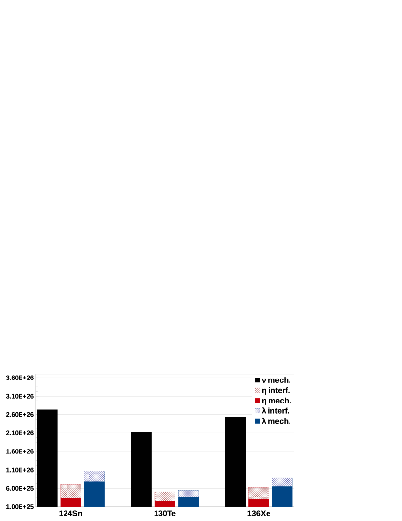
Figure 1: The calculated lifetimes and their uncertainties (the hatched bars) form the interference of the unknown CP phases.

The shapes of the two-electron angular distributions of Eq. (8) could be used to distinguish between the mass mechanism and the $\lambda$ or the $\eta$ mechanisms. However, many recorded events (tens or more) are needed for a reliable evaluation, and even then one can face difficulties due to the unknown CP phases. The ¹²⁴Sn angular distribution is presented in Fig. 2. One can see that $\lambda$ (blue bands) and $\eta$ (red bands) exhibit similar shapes, differing in amplitude, and opposite to that of the mass mechanism (black line). In the case of ¹³⁰Te, the same is to be expected, but the $\lambda$ and $\eta$ bands overlap due to the unknown phases, as seen in Fig. 3. The ¹³⁶Xe angular distribution is very similar to that of ¹²⁴Sn and is presented in Fig. 4.

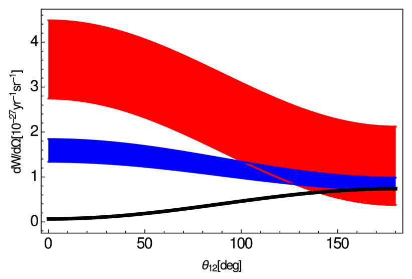
Figure 2: Electrons angular distribution for ¹²⁴Sn.

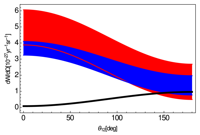
Figure 3: Electrons angular distribution for ¹³⁰Te.

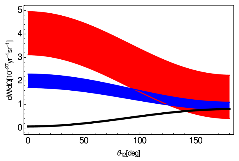
Figure 4: Electrons angular distribution for ¹³⁶Xe.

In principle, the $\lambda$ and the $\eta$ contributions could be identified in the shapes of the two-electron energy distributions. While the tails of the distributions (when the difference between the energy of one electron and that of the other is maximal) overlap, the starting points (when both electrons have almost equal energies) are very different for the $\lambda$ from the $\eta$ mechanism. Fig. 5 shows the energy distribution for ¹²⁴Sn. The ¹³⁰Te energy distribution is presented in Fig. 6. For ¹³⁶Xe we find an energy distribution very similar to that of ¹²⁴Sn, like in the case of the angular distributions.

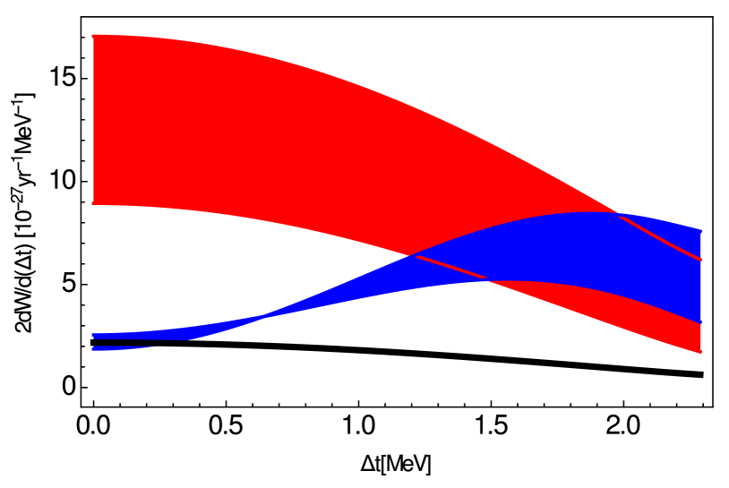
Figure 5: Electrons energy distribution for ¹²⁴Sn.

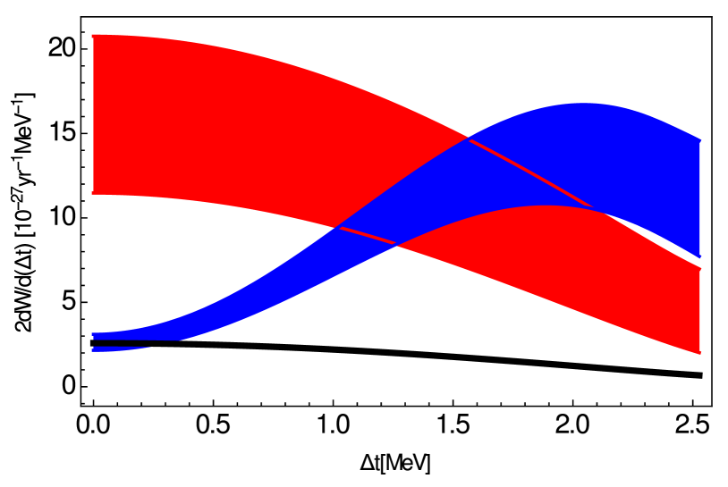
Figure 6: Electrons energy distribution for ¹³⁰Te.

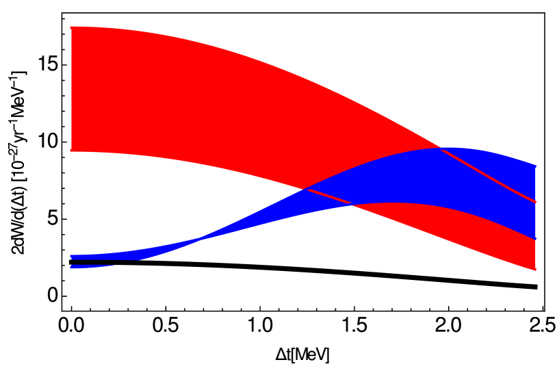
Figure 7: Electrons energy distribution for ¹³⁶Xe.

To further aid with the disentanglement of the $\lambda$ and $\eta$ mechanisms, we provide plots of the angular correlation coefficient, $\alpha=B(\epsilon)/A(\epsilon)$ in our Eq. (4). This may help reduce the uncertainties induced by the unknown CP phases (see e.g. Figs. 6.5 - 6.9 of Doi et al. (1985) and Fig. 7 of Stefanik et al. (2015)). From $\alpha(\Delta t)$, one may also obtain a clearer separation from the mass mechanism over a wide range of energies. The angular correlation coefficient for ¹²⁴Sn is presented in Fig. 8. The same behavior can be identified in Fig. 9 for ¹³⁰Te and in Fig. 10 for ¹³⁶Xe.

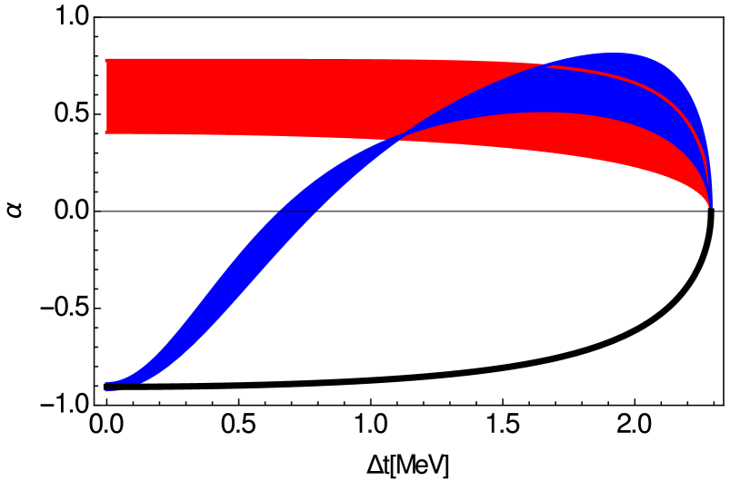
Figure 8: The angular correlation coefficient for ¹²⁴Sn.

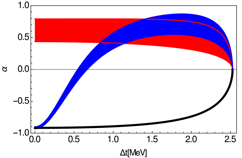
Figure 9: The angular correlation coefficient for ¹³⁰Te.

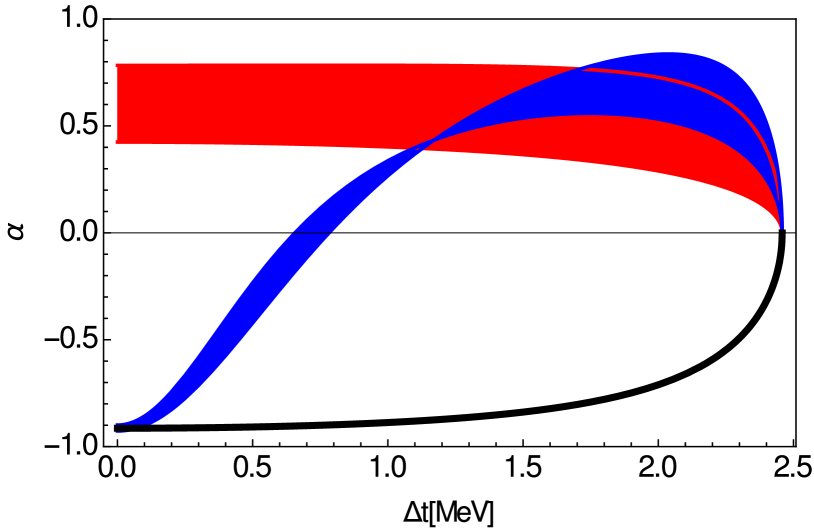
Figure 10: The angular correlation coefficient for ¹³⁶Xe.

IV Conclusions

In this paper we report shell model calculations necessary to disentangle the mixed right-handed/left-handed currents contributions (commonly referred to as $\eta$ and $\lambda$ mechanisms) from the mass mechanism in the left-right symmetric model. We perform an analysis of these contributions by considering three theoretical scenarios, one for the mass mechanism, another for the $\lambda$ dominance in competition with the mass mechanism, and a scenario where the $\eta$ mechanism dominates in competition with the mass mechanism.

The figures presented support the conclusions Doi et al. (1985); Horoi and Neacsu (2016a) that one can distinguish the $\lambda$ or $\eta$ dominance over the mass mechanism from the shape of the two-electron angular distribution, while one can discriminate the $\lambda$ from the $\eta$ mechanism using the shape of the energy distribution and that of the angular coefficient. The tables and the figures presented also show the uncertainties related to the effects of interference from the unknown CP-violating phases.

We show our results for phase space factors, nuclear matrix elements and lifetimes for $0\nu\beta\beta$ transitions of ¹²⁴Sn, ¹³⁰Te, and ¹³⁶Xe to ground states. In the case of the mass mechanism nuclear matrix elements, we obtain results which are consistent with previous calculations Neacsu and Horoi (2015b); Horoi and Neacsu (2016a), where the same SVD Hamiltonian was used. Similar to the case of ⁸²Se Horoi and Neacsu (2016a), the inclusion of the $\eta$ and $\lambda$ mechanisms contributions tends to decrease the half-lives.

The phase-space factors included in the analysis of life-times and two-electron distributions are calculated using a recently proposed accurate effective method Neacsu and Horoi (2015a) that provides results very close to those of Ref. Stefanik et al. (2015). Ref. Stefanik et al. (2015) takes into account consistently the effects of the realistic finite size proton distribution in the daughter nucleus, but it does not provide all the energy-dependent phase-space contributions necessary for our analysis.

Consistent with the calculations and conclusions we obtained for ⁸²Se Horoi and Neacsu (2016a), if the $\eta$ mechanism exists, it may be favored to compete with the mass mechanisms because of the larger contribution from the phase space factors.

Finally, we conclude that in experiments where outgoing electrons can be tracked, this analysis is possible if enough data is collected, generally of the order of a few tens of events. This may be beyond the realistic capabilities of the current experiments, but should a positive neutrinoless double-beta decay measurement be achieved, it is expected that more resources could be allocated to improve the statistics and the variety of investigated isotopes.