On the Consistency of the Likelihood Maximization Vertex Nomination Scheme: Bridging the Gap Between Maximum Likelihood Estimation and Graph Matching

Abstract

Given a graph in which a few vertices are deemed interesting a priori, the vertex nomination task is to order the remaining vertices into a nomination list such that there is a concentration of interesting vertices at the top of the list. Previous work has yielded several approaches to this problem, with theoretical results in the setting where the graph is drawn from a stochastic block model (SBM), including a vertex nomination analogue of the Bayes optimal classifier. In this paper, we prove that maximum likelihood (ML)-based vertex nomination is consistent, in the sense that the performance of the ML-based scheme asymptotically matches that of the Bayes optimal scheme. We prove theorems of this form both when model parameters are known and unknown. Additionally, we introduce and prove consistency of a related, more scalable restricted-focus ML vertex nomination scheme. Finally, we incorporate vertex and edge features into ML-based vertex nomination and briefly explore the empirical effectiveness of this approach.

1 Introduction and Background

Graphs are a common data modality, useful for modeling complex relationships between objects, with applications spanning fields as varied as biology (Jeong et al., 2001; Bullmore and Sporns, 2009), sociology (Wasserman and Faust, 1994), and computer vision (Foggia et al., 2014; Kandel et al., 2007), to name a few. For example, in neuroscience, vertices may be neurons and edges adjoin pairs of neurons that share a synapse (Bullmore and Sporns, 2009); in social networks, vertices may correspond to people and edges to friendships between them (Carrington et al., 2005; Yang and Leskovec, 2015); in computer vision, vertices may represent pixels in an image and edges may represent spatial proximity or multi-resolution mappings (Kandel et al., 2007). In many useful networks, vertices with similar attributes form densely-connected communities compared to vertices with highly disparate attributes, and uncovering these communities is an important step in understanding the structure of the network. There is an extensive literature devoted to uncovering this community structure in network data, including methods based on maximum modularity (Newman and Girvan, 2004; Newman, 2006b), spectral partitioning algorithms (Luxburg, 2007; Rohe et al., 2011; Sussman et al., 2012; Lyzinski et al., 2014b), and likelihood-based methods (Bickel and Chen, 2009), among others.

In the setting of vertex nomination, one community in the network is of particular interest, and the inference task is to order the vertices into a nomination list with those vertices from the community of interest concentrating at the top of the list. See Marchette et al. (2011); Coppersmith and Priebe (2012); Coppersmith (2014); Fishkind et al. (2015) and the references contained therein for a review of the relevant vertex nomination literature. Vertex nomination is a semi-supervised inference task, with example vertices from the community of interest—and, ideally, also examples not from the community of interest—being leveraged in order to create a nomination list. In this way, the vertex nomination problem is similar to the problem faced by personalized recommender systems (see, for example, Resnick and Varian, 1997; Ricci et al., 2011), where, given a training list of objects of interest, the goal is to arrange the remaining objects into a recommendation list with “interesting” objects concentrated at the top of the list. The main difference between the two inference tasks is that in vertex nomination the features of the data are encoded into the topology of a network, rather than being observed directly as features (though see Section 5 for the case where vertices are annotated with additional information in the form of features).

In this paper, we develop the notion of a consistent vertex nomination scheme (Definition 2). We then proceed to prove that the maximum likelihood vertex nomination scheme of Fishkind et al. (2015) is consistent under mild model assumptions on the underlying stochastic block model (Theorem 6). In the process, we propose a new, efficiently exactly solvable likelihood-based vertex nomination scheme, the restricted-focus maximum likelihood vertex nomination scheme, $\mathcal{L}^{\operatorname{ML}}_{R}$, and prove the analogous consistency result (Theorem 8). In addition, under mild model assumptions, we prove that both schemes maintain their consistency when the stochastic block model parameters are unknown and are estimated using the seed vertices (Theorems 9 and 10). In both cases, we show that consistency is possible even when the seeds are an asymptotically vanishing portion of the graph. Lastly, we show how both schemes can be easily modified to incorporate edge weights and vertex features (Section 5), before demonstrating the practical effect of our theoretical results on real and synthetic data (Section 6) and closing with a brief discussion (Section 7).

Notation: We say that a sequence of random variables $(X_{n})_{n=1}^{\infty}$ converges almost surely to random variable $X$, written $X_{n}\rightarrow X$ a.s., if $\mathbb{P}[\lim_{n\rightarrow\infty}X_{n}=X]=1$. We say a sequence of events $(A_{n})_{n=1}^{\infty}$ occurs almost always almost surely (abbreviated a.a.a.s.) if with probability 1, $A_{n}^{c}$ occurs for at most finitely many $n$. By the Borel-Cantelli lemma, $\sum_{n=1}^{\infty}\mathbb{P}[A_{n}^{c}]<\infty$ implies $(A_{n})_{n=1}^{\infty}$ occurs a.a.a.s. We write $\mathcal{G}_{n}$ to denote the set of all (possibly weighted) graphs on $n$ vertices. Throughout, without loss of generality, we will assume that the vertex set is given by $V=\{1,2,\dots,n\}$. For a positive integer $K$, we will often use $[K]$ to denote the set $\{1,2,\dots,K\}$. For a set $V$, we will use $\binom{V}{2}$ to denote the set of all pairs of distinct elements of $V$. That is, $\binom{V}{2}=\{\{u,v\}:u,v\in V,u\neq v\}$. For a function $f$ with domain $V$, we write $f_{|_{U}}$ to denote the restriction of $f$ to the set $U\subset V$.

1.1 Background

Stochastic block model random graphs offer a theoretically tractable model for graphs with latent community structure (Rohe et al., 2011; Sussman et al., 2012; Bickel and Chen, 2009), and have been widely used in the literature to model community structure in real networks (Airoldi et al., 2008; Karrer and Newman, 2011). While stochastic block models can be too simplistic to capture the eccentricities of many real graphs, they have proven to be a useful, tractable surrogate for more complicated networks (Airoldi et al., 2013; Olhede and Wolfe, 2014).

Definition 1.

Let $K$ and $n$ be positive integers and let $\vec{n}=(n_{1},n_{2},\dots,n_{K})^{\top}\in\mathbb{R}^{K}$ be a vector of positive integers with $\sum_{k}n_{k}=n$. Let $b:[n]\rightarrow[K]$ and let $\Lambda\in[0,1]^{K\times K}$ be symmetric. A $\mathcal{G}_{n}$-valued random graph $G$ is an instantiation of a $(K,\vec{n},b,\Lambda)$ conditional Stochastic Block Model, written $G\sim\operatorname{SBM}(K,\vec{n},b,\Lambda)$, if

• The vertex set $V$ is partitioned into $K$ blocks, $V_{1},V_{2},\dots,V_{K}$ of cardinalities $|V_{k}|=n_{k}$ for $k=1,2,\dots,K$;

• The block membership function $b:V\rightarrow[K]$ is such that for each $v\in V$, $v\in V_{b(v)}$;

• The symmetric block communication matrix $\Lambda\in[0,1]^{K\times K}$ is such that for each $\{v,u\}\in\binom{V}{2}$, there is an edge between vertices $u$ and $v$ with probability $\Lambda_{b(u),b(v)}$, independently of all other edges.

Without loss of generality, let $V_{1}$ be the block of interest for vertex nomination. For each $k\in[K]$, we further decompose $V_{k}$ into $V_{k}=S_{k}\cup U_{k}$ (with $|S_{k}|=m_{k}$), where the vertices in $S:=\cup_{k}S_{k}$ have their block membership observed a priori. We call the vertices in $S$ seed vertices, and let $m=|S|$. We will denote the set of nonseed vertices by $U=\cup_{k}U_{k}$, and for all $k\in[K]$, let $\mathfrak{u}_{k}:=n_{k}-m_{k}=|U_{k}|$ and $n-m=\mathfrak{u}=|U|.$ Throughout this paper, we assume that the seed vertices $S$ are chosen uniformly at random from all possible subsets of $V$ of size $m$. The task in vertex nomination is to leverage the information contained in the seed vertices to produce a nomination list $\mathcal{L}:U\rightarrow[\mathfrak{u}]$ (i.e., an ordering of the vertices in $U$) such that the vertices in $U_{1}$ concentrate at the top of the list. We note that, strictly speaking, a nomination list $\mathcal{L}$ is also a function of the observed graph $G$, a fact that we suppress for ease of notation. We measure the efficacy of a nomination scheme via average precision

$$\operatorname{AP}(\mathcal{L})=\frac{1}{\mathfrak{u}_{1}}\sum_{i=1}^{\mathfrak{u}_{1}}\frac{\sum_{j=1}^{i}\mathbbm{1}\{\mathcal{L}^{-1}(j)\in U_{1}\}}{i}.$$ (1)

AP ranges from $0$ to $1$, with a higher value indicating a more effective nomination scheme: indeed, $\operatorname{AP}(\mathcal{L})=1$ indicates that the first $\mathfrak{u}_{1}$ vertices in the nomination list are all from the block of interest, and $\operatorname{AP}(\mathcal{L})=0$ indicates that none of the $\mathfrak{u}_{1}$ top-ranked vertices are from the block of interest. Letting $H_{k}=\sum_{j=1}^{k}1/j$ denote the $k$-th harmonic number, with the convention that $H_{0}=0$, we can rearrange (1) as

$$\operatorname{AP}(\mathcal{L})=\sum_{i=1}^{\mathfrak{u}_{1}}\frac{H_{\mathfrak{u}_{1}}-H_{i-1}}{\mathfrak{u}_{1}}\mathbbm{1}\{\mathcal{L}^{-1}(i)\in U_{1}\},$$

from which we see that the average precision is simply a convex combination of the indicators of correctness in the rank list, in which correctly placing an interesting vertex higher in the nomination list (i.e., with rank close to 1) is rewarded more than correctly placing an interesting vertex lower in the nomination list.

In Fishkind et al. (2015), three vertex nomination schemes are presented in the context of stochastic block model random graphs: the canonical vertex nomination scheme, $\mathcal{L}^{\operatorname{C}}$, which is suitable for small graphs (tens of vertices); the likelihood maximization vertex nomination scheme, $\mathcal{L}^{\operatorname{ML}}$, which is suitable for small to medium graphs (up to thousands of vertices); and the spectral partitioning vertex nomination scheme, $\mathcal{L}^{\operatorname{SP}}$, which is suitable for medium to very large graphs (up to tens of millions of vertices). In the stochastic block model setting, the canonical vertex nomination scheme is provably optimal: under mild model assumptions, $\mathbb{E}\operatorname{AP}(\mathcal{L}^{\operatorname{C}})\geq\mathbb{E}\operatorname{AP}(\mathcal{L})$ for any vertex nomination scheme $\mathcal{L}$ (Fishkind et al., 2015), where the expectation is with respect to a $\mathcal{G}_{m+n}$-valued random graph $G$ and the selection of the seed vertices. Thus, the canonical method is the vertex nomination analogue of the Bayes classifier, and this motivates the following definition:

Definition 2.

Let $G\sim\operatorname{SBM}(K,\vec{n},b,\Lambda)$. With notation as above, a vertex nomination scheme $\mathcal{L}$ is consistent if

$$\lim_{n\rightarrow\infty}|\mathbb{E}\operatorname{AP}(\mathcal{L}^{C})-\mathbb{E}\operatorname{AP}(\mathcal{L})|=0.$$

In our proofs below, where we establish the consistency of two nomination schemes, we prove a stronger fact, namely that $\operatorname{AP}(\mathcal{L})=1$ a.a.a.s. We prefer the definition of consistency given in Definition 2 since it allows us to speak about the best possible nomination scheme even when the model is such that $\lim_{n\rightarrow\infty}\mathbb{E}\operatorname{AP}(\mathcal{L}^{\operatorname{C}})<1$.

In Fishkind et al. (2015), it was proven that under mild assumptions on the stochastic block model underlying $G$, we have

$$\lim_{n\rightarrow\infty}\mathbb{E}\operatorname{AP}(\mathcal{L}^{\operatorname{SP}})=1,$$

from which the consistency of $\mathcal{L}^{\operatorname{SP}}$ follows immediately. The spectral nomination scheme $\mathcal{L}^{\operatorname{SP}}$ proceeds by first $K$-means clustering the adjacency spectral embedding (Sussman et al., 2012) of $G$, and then nominating vertices based on their distance to the cluster of interest. Consistency of $\mathcal{L}^{\operatorname{SP}}$ is an immediate consequence of the fact that, under mild model assumptions on the underlying stochastic block model, $K$-means clustering of the adjacency spectral embedding of $G$ perfectly clusters the vertices of $G$ a.a.a.s. (Lyzinski et al., 2014b).

Bickel and Chen (2009) proved that maximum likelihood estimation provides consistent estimates of the model parameters in a more common variant of the conditional stochastic block model of Definition 1, namely, in the stochastic block model with random block assignments:

Definition 3.

Let $K,n$ and $\Lambda$ be as above. Let $\vec{\pi}=\pi_{1},\pi_{2},\ldots,\pi_{K})^{\top}\in\Delta^{K-1}$ be a probability vector over $K$ outcomes and let $\tau:V\rightarrow[K]$ be a random function. A $\mathcal{G}_{n}$-valued random graph $G$ is an instantiation of a $(K,\vec{\pi},\tau,\Lambda)$ Stochastic Block Model with random block assignments, written $G\sim\operatorname{SBM}(K,\vec{\pi},\tau,\Lambda)$, if

• For each vertex $v\in V$ and block $k\in[K]$, independently of all other vertices, the block assignment function $\tau:V\rightarrow[K]$ assigns $v$ to block $k$ with probability $\pi_{k}$ (i.e., $\mathbb{P}[\tau(v)=k]=\pi_{k}$);

• The symmetric block communication matrix $\Lambda\in[0,1]^{K\times K}$ is such that, conditioned on $\tau$, for each $\{v,u\}\in\binom{V}{2}$ there is an edge between vertices $u$ and $v$ with probability $\Lambda_{\tau(u),\tau(v)}$, independently of all other edges.

A consequence of the result of Bickel and Chen (2009) is that the maximum likelihood estimate of the block assignment function perfectly clusters the vertices a.a.a.s. in the setting where $G\sim\operatorname{SBM}(K,\vec{\pi},\tau,\Lambda)$. This bears noting, as our maximum likelihood vertex nomination schemes $\mathcal{L}^{\operatorname{ML}}$ and $\mathcal{L}^{\operatorname{ML}}_{R}$ (defined below in Section 2) proceed by first constructing a maximum likelihood estimate of the block membership function $b$, then ranking vertices based on a measure of model misspecification. Extending the results from Bickel and Chen (2009) to our present framework—where we consider $\Lambda$ and $\vec{n}$ to be known (or errorfully estimated via seeded vertices) as opposed to parameters to be optimized over in the likelihood function as done in Bickel and Chen (2009)—is not immediate.

We note the recent result by Newman (2016), which shows the equivalence of maximum-likelihood and maximum modularity methods in a special case of the stochastic block model when $\Lambda$ is known. Our results, along with this recent result, immediately imply a consistent maximum modularity-based vertex nomination scheme under that special-case model.

2 Graph Matching and Maximum Likelihood Estimation

Consider $G\sim\operatorname{SBM}(K,\vec{n},b,\Lambda)$ with associated adjacency matrix $A$, and, as above, denote the set of seed vertices by $S=\cup_{k}S_{k}$. Define the set of feasible block assignment functions

$$\mathcal{B} =\mathcal{B}(\vec{n},b,S)$$

$$:=\{\phi:V\rightarrow[K]\text{ s.t. for all }k\in[K],\,|\phi^{-1}(k)|=n_{k},\text{ and }\phi(i)=b(i)\text{ for all }i\in S\}.$$

The maximum likelihood estimator of $b\in\mathcal{B}$ is any member of the set of functions

$$\hat{b} =\arg\max_{\phi\in\mathcal{B}}\prod_{\{i,j\}\in\binom{V}{2}}\Lambda_{\phi(i),\phi(j)}^{A_{i,j}}(1-\Lambda_{\phi(i),\phi(j)})^{1-A_{i,j}}$$

$$=\arg\max_{\phi\in\mathcal{B}}\sum_{\{i,j\}\in\binom{V}{2}}A_{i,j}\log\left(\frac{\Lambda_{\phi(i),\phi(j)}}{1-\Lambda_{\phi(i),\phi(j)}}\right)$$

$$=\arg\max_{\phi\in\mathcal{B}}\sum_{\{i,j\}\in\binom{U}{2}}A_{i,j}\log\left(\frac{\Lambda_{\phi(i),\phi(j)}}{1-\Lambda_{\phi(i),\phi(j)}}\right)+\sum_{(i,j)\in S\times U}A_{i,j}\log\left(\frac{\Lambda_{b(i),\phi(j)}}{1-\Lambda_{b(i),\phi(j)}}\right),$$ (2)

where the second equality follows from independence of the edges and splitting the edges in the sum according to whether or not they are incident to a seed vertex. We can reformulate (2) as a graph matching problem by identifying $\phi$ with a permutation matrix $P$:

Definition 4.

Let $G_{1}$ and $G_{2}$ be two $n$-vertex graphs with respective adjacency matrices $A$ and $B$. The Graph Matching Problem for aligning $G_{1}$ and $G_{2}$ is

$$\min_{P\in\Pi_{n}}\|AP-PB\|_{F},$$

where $\Pi_{n}$ is defined to be the set of all $n\times n$ permutation matrices.

Incorporating seed vertices (i.e., vertices whose correspondence across $G_{1}$ and $G_{2}$ is known a priori) into the graph matching problem is immediate (Fishkind et al., 2012). Letting the seed vertices be (without loss of generality) $S=\{1,2,\dots,m\}$ in both graphs, the seeded graph matching (SGM) problem is

$$\min_{P\in\Pi_{\mathfrak{u}}}\left\|A(I_{m}\oplus P)-(I_{m}\oplus P)B\right\|_{F},$$ (3)

where

$$I_{m}\oplus P=\begin{bmatrix}I_{m}&0\\ 0&P\end{bmatrix}.$$

Setting $B\in\mathbb{R}^{n\times n}$ to be the log-odds matrix

$$B_{i,j}:=\log\Bigg{(}\frac{\Lambda_{b(i),b(j)}}{1-\Lambda_{b(i),b(j)}}\Bigg{)},$$ (4)

observe that the optimization problem in Equation (2) is equivalent to that in (3) if we view $B$ as encoding a weighted graph. Hence, we can apply known graph matching algorithms to approximately find $\hat{b}$.

Decomposing $A$ and $B$ as

$$A=\hbox{}\vbox{\kern 0.86108pt\hbox{$\kern 0.0pt\kern 2.5pt\kern-5.0pt\left[\kern 0.0pt\kern-2.5pt\kern-5.55557pt\vbox{\kern-0.86108pt\vbox{\vbox{ \halign{\kern\arraycolsep\hfil\@arstrut$\kbcolstyle#$\hfil\kern\arraycolsep& \kern\arraycolsep\hfil$\@kbrowstyle#$\ifkbalignright\relax\else\hfil\fi\kern\arraycolsep&& \kern\arraycolsep\hfil$\@kbrowstyle#$\ifkbalignright\relax\else\hfil\fi\kern\arraycolsep\cr 5.0pt\hfil\@arstrut$\scriptstyle$\hfil\kern 5.0pt&5.0pt\hfil$\scriptstyle m$\hfil\kern 5.0pt&5.0pt\hfil$\scriptstyle\mathfrak{u}\\m$\hfil\kern 5.0pt&5.0pt\hfil$\scriptstyle A^{(1,1)}$\hfil\kern 5.0pt&5.0pt\hfil$\scriptstyle A^{(1,2)}\\\mathfrak{u}$\hfil\kern 5.0pt&5.0pt\hfil$\scriptstyle A^{(2,1)}$\hfil\kern 5.0pt&5.0pt\hfil$\scriptstyle A^{(2,2)})$\hfil\kern 5.0pt\crcr}}}}\right]$}}\hskip 28.45274ptB=\hbox{}\vbox{\kern 0.86108pt\hbox{$\kern 0.0pt\kern 2.5pt\kern-5.0pt\left[\kern 0.0pt\kern-2.5pt\kern-5.55557pt\vbox{\kern-0.86108pt\vbox{\vbox{ \halign{\kern\arraycolsep\hfil\@arstrut$\kbcolstyle#$\hfil\kern\arraycolsep& \kern\arraycolsep\hfil$\@kbrowstyle#$\ifkbalignright\relax\else\hfil\fi\kern\arraycolsep&& \kern\arraycolsep\hfil$\@kbrowstyle#$\ifkbalignright\relax\else\hfil\fi\kern\arraycolsep\cr 5.0pt\hfil\@arstrut$\scriptstyle$\hfil\kern 5.0pt&5.0pt\hfil$\scriptstyle m$\hfil\kern 5.0pt&5.0pt\hfil$\scriptstyle\mathfrak{u}\\m$\hfil\kern 5.0pt&5.0pt\hfil$\scriptstyle B^{(1,1)}$\hfil\kern 5.0pt&5.0pt\hfil$\scriptstyle B^{(1,2)}\\\mathfrak{u}$\hfil\kern 5.0pt&5.0pt\hfil$\scriptstyle B^{(2,1)}$\hfil\kern 5.0pt&5.0pt\hfil$\scriptstyle B^{(2,2)}$\hfil\kern 5.0pt\crcr}}}}\right]$}}$$

and using the fact that $P\in\Pi_{n}$ is unitary, the seeded graph matching problem is equivalent (i.e., has the same minimizer) to

$$\min_{P\in\Pi_{\mathfrak{u}}}-\operatorname{tr}\left(A^{(2,2)}P(B^{(2,2)})^{\top}P^{\top}\right)-\operatorname{tr}\left((A^{(1,2)})^{\top}B^{(1,2)}P^{\top}\right)-\operatorname{tr}\left(A^{(2,1)}(B^{(2,1)})^{\top}P^{\top}\right).$$

Thus, we can recast (2) as a seeded graph matching problem so that finding

$$\hat{b} =\arg\max_{\phi\in\mathcal{B}}\sum_{\{i,j\}\in\binom{U}{2}}A_{i,j}\log\left(\frac{\Lambda_{\phi(i),\phi(j)}}{1-\Lambda_{\phi(i),\phi(j)}}\right)+\sum_{(i,j)\in S\times U}A_{i,j}\log\left(\frac{\Lambda_{b(i),\phi(j)}}{1-\Lambda_{b(i),\phi(j)}}\right)$$

is equivalent to finding

$$\hat{P} =\arg\min_{P\in\Pi_{\mathfrak{u}}}-\frac{1}{2}\operatorname{tr}\left(A^{(2,2)}P(B^{(2,2)})^{\top}P^{\top}\right)-\operatorname{tr}\left((A^{(1,2)})^{\top}B^{(1,2)}P^{\top}\right),$$ (5)

as we shall explain below.

With $B$ defined as in (4), we define

$$\mathcal{Q}=\left\{Q\in\Pi_{\mathfrak{u}}\text{ s.t. }(I_{m}\oplus Q)B(I_{m}\oplus Q)^{\top}=B\right\}.$$

Define an equivalence relation $\sim$ on $\Pi_{\mathfrak{u}}$ via $P_{1}\sim P_{2}$ iff there exists a $Q\in\mathcal{Q}$ such that $P_{1}=P_{2}Q$; i.e.,

$$(I_{m}\oplus P_{1})B(I_{m}\oplus P_{1})^{\top}=(I_{m}\oplus P_{2}Q)B(I_{m}\oplus P_{2}Q)^{\top}=(I_{m}\oplus P_{2})B(I_{m}\oplus P_{2})^{\top}.$$

Let $\hat{P}/\sim$ denote the set of equivalence classes of $\hat{P}$ under equivalence relation $\sim$. Solving (2) is equivalent to solving (5) in that there is a one-to-one correspondence between $\hat{b}$ and $\hat{P}/\sim$: for each $\phi\in\hat{b}$ there is a unique $P\in\hat{P}/\sim$ (with associated permutation $\sigma$) such that $\phi_{|_{U}}=b_{|_{U}}\circ\sigma$; and for each $P\in\hat{P}/\sim$ (with the permutation associated with $I_{m}\oplus P$ given by $\sigma$), it holds that $b\circ\sigma\in\hat{b}$.

2.1 The $\mathcal{L}^{\operatorname{ML}}$ Vertex Nomination Scheme

The maximum likelihood (ML) vertex nomination scheme proceeds as follows. First, the SGM algorithm (Fishkind et al., 2012; Lyzinski et al., 2014a) is used to approximately find an element of $\hat{P}$, which we shall denote by $P$. Let the corresponding element of $\hat{b}$ be denoted by $\phi$. For any $i,j\in V$ such that $\phi(i)\neq\phi(j)$, define $\phi_{i\leftrightarrow j}\in\mathcal{B}$ as

$$\phi_{i\leftrightarrow j}(v)=\begin{cases}\phi(i)&\text{ if }v=j,\\ \phi(j)&\text{ if }v=i,\\ \phi(v)&\text{ if }v\neq i,j;\end{cases}$$

i.e., $\phi_{i\leftrightarrow j}$ agrees with $\phi$ except that $i$ and $j$ have their block memberships from $\phi$ switched in $\phi_{i\leftrightarrow j}$. For $i\in U$ such that $\phi(i)=1$, define

$$\eta(i):=\left(\prod_{\begin{subarray}{c}j\in U\text{ s.t.}\\ \phi(j)\neq 1\end{subarray}}\frac{\ell(\phi_{i\leftrightarrow j},G)}{\ell(\phi,G)}\right)^{\frac{1}{\mathfrak{u}-\mathfrak{u}_{1}}},$$

where, for each $\psi\in\mathcal{B}$, the likelihood $\ell$ is given by

$$\ell(\psi,G)=\prod_{\{i,j\}\in\binom{U}{2}}\Lambda_{\psi(i),\psi(j)}^{A_{i,j}}(1-\Lambda_{\psi(i),\psi(j)})^{1-A_{i,j}}\prod_{(i,j)\in S\times U}\Lambda_{b(i),\psi(j)}^{A_{i,j}}(1-\Lambda_{b(i),\psi(j)})^{1-A_{i,j}}.$$

A low/high value of $\eta(i)$ is a measure of our confidence that $i$ is/is not in the block of interest. For $i\in U$ such that $\phi(i)\neq 1$, define

$$\xi(i):=\left(\prod_{\begin{subarray}{c}j\in U\text{ s.t.}\\ \phi(j)=1\end{subarray}}\frac{\ell(\phi_{i\leftrightarrow j},G)}{\ell(\phi,G)}\right)^{\frac{1}{\mathfrak{u}_{1}}}.$$

A low/high value of $\xi(i)$ is a measure of our confidence that $i$ is/is not in the block of interest. We are now ready to define the maximum-likelihood based nomination scheme $\mathcal{L}^{\operatorname{ML}}$:

$$\left(\mathcal{L}^{\operatorname{ML}}\right)^{-1}(1) \in\arg\min\{\eta(v):\phi(v)=1\}$$

$$\left(\mathcal{L}^{\operatorname{ML}}\right)^{-1}(2) \in\arg\min\left\{\eta(v):v\in U\setminus\left\{(\mathcal{L}^{\operatorname{ML}})^{-1}(1)\right\},\phi(v)=1\right\}$$

$$\vdots$$

$$\left(\mathcal{L}^{\operatorname{ML}}\right)^{-1}(\mathfrak{u}_{1}) \in\arg\min\left\{\eta(v):v\in U\setminus\left\{(\mathcal{L}^{\operatorname{ML}})^{-1}(i)\right\}_{i=1}^{\mathfrak{u}_{1}-1},\phi(v)=1\right\}$$

$$\left(\mathcal{L}^{\operatorname{ML}}\right)^{-1}(\mathfrak{u}_{1}+1) \in\arg\max\left\{\xi(v):\phi(v)\neq 1\right\}$$

$$\left(\mathcal{L}^{\operatorname{ML}}\right)^{-1}(\mathfrak{u}_{1}+2) \in\arg\max\left\{\xi(v):v\in U\setminus\left\{(\mathcal{L}^{\operatorname{ML}})^{-1}(\mathfrak{u}_{1}+1)\right\},\phi(v)\neq 1\right\}$$

$$\vdots$$

$$\left(\mathcal{L}^{\operatorname{ML}}\right)^{-1}(\mathfrak{u}) \in\arg\max\left\{\xi(v):v\in U\setminus\left\{(\mathcal{L}^{\operatorname{ML}})^{-1}(i)\right\}_{i=\mathfrak{u}_{1}+1}^{\mathfrak{u}-1},\phi(v)\neq 1\right\}$$

Note that in the event that an argmin (or argmax) above contains more than one element, the order in which these elements is nominated should be taken to be uniformly random.

Remark 5.

In the event that $\Lambda$ is unknown a priori, we can use the block memberships of the seeds $S$ (assumed to be chosen uniformly at random from $V$) to estimate the edge probability matrix $\Lambda$ as

$$\widehat{\Lambda}_{k,\ell}=\frac{|\{\{i,j\}\in E\text{ s.t. }i\in S_{k},\,j\in S_{\ell}\}|}{m_{k}m_{\ell}}\text{ for }k\neq\ell,$$

and

$$\widehat{\Lambda}_{k,k}=\frac{|\{\{i,j\}\in E\text{ s.t. }i\in S_{k},\,j\in S_{k}\}|}{\binom{m_{k}}{2}}.$$

The plug-in estimate $\widehat{B}$ of $B$, given by

$$\widehat{B}_{i,j}:=\log\left(\frac{\widehat{\Lambda}_{b(i),b(j)}}{1-\widehat{\Lambda}_{b(i),b(j)}}\right),$$

can then be used in place of $B$ in Eq. (5). If, in addition, $\vec{n}$ is unknown, we can estimate the block sizes $n_{k}$ as

$$\hat{n}_{k}=\frac{m_{k}n}{m},$$

for each $k\in[K]$, and these estimates can be used to determine the block sizes in $\widehat{B}$.

2.2 The $\mathcal{L}^{\operatorname{ML}}_{R}$ Vertex Nomination Scheme

Graph matching is a computationally difficult problem, and there are no known polynomial time algorithms for solving the general graph matching problem for simple graphs. Furthermore, if the graphs are allowed to be weighted, directed, and loopy, then graph matching is equivalent to the NP-hard quadratic assignment problem. While there are numerous efficient, approximate graph matching algorithms (see, for example, Vogelstein et al., 2014; Fishkind et al., 2012; Zaslavskiy et al., 2009; Fiori et al., 2013, and the references therein), these algorithms often lack performance guarantees.

Inspired by the restricted-focus seeded graph matching problem considered in Lyzinski et al. (2014a), we now define the computationally tractable restricted-focus likelihood maximization vertex nomination scheme $\mathcal{L}^{\operatorname{ML}}_{R}$. Rather than attempting to quickly approximate a solution to the full graph matching problem as in Vogelstein et al. (2014); Fishkind et al. (2012); Zaslavskiy et al. (2009); Fiori et al. (2013), this approach simplifies the problem by ignoring the edges between unseeded vertices. An analogous restriction for matching simple graphs was introduced in Lyzinski et al. (2014a). We begin by considering the graph matching problem in Eq. (5). The objective function

$$-\frac{1}{2}\operatorname{tr}\left(A^{(2,2)}P(B^{(2,2)})^{\top}P^{\top}\right)-\operatorname{tr}\left((A^{(1,2)})^{\top}B^{(1,2)}P^{\top}\right)$$

consists of two terms: $-\frac{1}{2}\operatorname{tr}\left(A^{(2,2)}P(B^{(2,2)})^{\top}P^{\top}\right),$ which seeks to align the induced subgraphs of the nonseed vertices; and $-\operatorname{tr}\left((A^{(1,2)})^{\top}B^{(1,2)}P^{\top}\right),$ which seeks to align the induced bipartite subgraphs between the seed and nonseed vertices. While the graph matching objective function, Eq. (5), is quadratic in $P$, restricting our focus to the second term in Eq. (5) yields the following linear assignment problem

$$\tilde{P} =\arg\min_{P\in\Pi_{\mathfrak{u}}}-\operatorname{tr}\left((A^{(1,2)})^{\top}B^{(1,2)}P^{\top}\right),$$ (6)

which can be efficiently and exactly solved in $O(\mathfrak{u}^{3})$ time with the Hungarian algorithm (Kuhn, 1955; Jonker and Volgenant, 1987). We note that, exactly as was the case of $\hat{P}$ and $\hat{b}$, finding $\tilde{P}$ is equivalent to finding

$$\tilde{b} =\arg\max_{\phi\in\mathcal{B}}\sum_{(i,j)\in S\times U}A_{i,j}\log\left(\frac{\Lambda_{b(i),\phi(j)}}{1-\Lambda_{b(i),\phi(j)}}\right),$$

in that there is a one-to-one correspondence between $\tilde{b}$ and $\tilde{P}/\sim$.

The $\mathcal{L}^{\operatorname{ML}}_{R}$ scheme proceeds as follows. First, the linear assignment problem, Eq. (6), is exactly solved using, for example, the Hungarian algorithm (Kuhn, 1955) or the path augmenting algorithm of Jonker and Volgenant (1987), yielding $P\in\tilde{P}$. Let the corresponding element of $\tilde{b}$ be denoted by $\phi.$ For $i\in U$ such that $\phi(i)=1$, define

$$\tilde{\eta}(i):=\left(\prod_{\begin{subarray}{c}j\in U\text{ s.t.}\\ \phi(j)\neq 1\end{subarray}}\frac{\ell_{R}(\phi_{i\leftrightarrow j},G)}{\ell_{R}(\phi,G)}\right)^{\frac{1}{\mathfrak{u}-\mathfrak{u}_{1}}},$$

where, for each $\psi\in\mathcal{B}$, the restricted likelihood $\ell_{R}$ is defined via

$$\ell_{R}(\psi,G)=\prod_{(i,j)\in S\times U}\Lambda_{b(i),\psi(j)}^{A_{i,j}}(1-\Lambda_{b(i),\psi(j)})^{1-A_{i,j}}.$$

As with $\mathcal{L}^{\operatorname{ML}},$ a low/high value of $\tilde{\eta}(i)$ is a measure of our confidence that $i$ is/is not in the block of interest. For $i\in U$ such that $\phi(i)\neq 1$, define

$$\tilde{\xi}(i):=\left(\prod_{\begin{subarray}{c}j\in U\text{ s.t.}\\ \phi(j)=1\end{subarray}}\frac{\ell_{R}(\phi_{i\leftrightarrow j},G)}{\ell_{R}(\phi,G)}\right)^{\frac{1}{\mathfrak{u}_{1}}}.$$

As before, a low/high value of $\tilde{\xi}(i)$ is a measure of our confidence that $i$ is/is not in the block of interest. We are now ready to define $\mathcal{L}^{\operatorname{ML}}_{R}$:

$$\left(\mathcal{L}^{\operatorname{ML}}_{R}\right)^{-1}(1) \in\arg\min\{\tilde{\eta}(v):\phi(v)=1\}$$

$$\left(\mathcal{L}^{\operatorname{ML}}_{R}\right)^{-1}(2) \in\arg\min\left\{\tilde{\eta}(v):v\in U\setminus\left\{(\mathcal{L}^{\operatorname{ML}}_{R})^{-1}(1)\right\},\phi(v)=1\right\}$$

$$\vdots$$

$$\left(\mathcal{L}^{\operatorname{ML}}_{R}\right)^{-1}(\mathfrak{u}_{1}) \in\arg\min\left\{\tilde{\eta}(v):v\in U\setminus\left\{(\mathcal{L}^{\operatorname{ML}}_{R})^{-1}(i)\right\}_{i=1}^{\mathfrak{u}_{1}-1},\phi(v)=1\right\}$$

$$\left(\mathcal{L}^{\operatorname{ML}}_{R}\right)^{-1}(\mathfrak{u}_{1}+1) \in\arg\max\left\{\tilde{\xi}(v):\phi(v)\neq 1\right\}$$

$$\left(\mathcal{L}^{\operatorname{ML}}_{R}\right)^{-1}(\mathfrak{u}_{1}+2) \in\arg\max\left\{\tilde{\xi}(v):v\in U\setminus\left\{(\mathcal{L}^{\operatorname{ML}}_{R})^{-1}(\mathfrak{u}_{1}+1)\right\},\phi(v)\neq 1\right\}$$

$$\vdots$$

$$\left(\mathcal{L}^{\operatorname{ML}}_{R}\right)^{-1}(\mathfrak{u}) \in\arg\max\left\{\tilde{\xi}(v):v\in U\setminus\left\{(\mathcal{L}^{\operatorname{ML}}_{R})^{-1}(i)\right\}_{i=\mathfrak{u}_{1}+1}^{\mathfrak{u}-1},\phi(v)\neq 1\right\}$$

Note that, as before, in the event that the argmin (or argmax) in the definition of $\mathcal{L}^{\operatorname{ML}}_{R}$ contains more than one element above, the order in which these elements are nominated should be taken to be uniformly random.

Unlike $\mathcal{L}^{\operatorname{ML}},$ the restricted focus scheme $\mathcal{L}^{\operatorname{ML}}_{R}$ is feasible even for comparatively large graphs (up to thousands of nodes, in our experience). However, we will see in Section 6 that the extra information available to $\mathcal{L}^{\operatorname{ML}}$—the adjacency structure among the nonseed vertices—leads to superior precision in the $\mathcal{L}^{\operatorname{ML}}$ nomination lists as compared to $\mathcal{L}^{\operatorname{ML}}_{R}$. We next turn our attention to proving the consistency of the $\mathcal{L}^{\operatorname{ML}}$ and $\mathcal{L}^{\operatorname{ML}}_{R}$ schemes.

3 Consistency of $\mathcal{L}^{\operatorname{ML}}$ and $\mathcal{L}^{\operatorname{ML}}_{R}$

In this section, we state theorems ensuring the consistency of the vertex nomination schemes $\mathcal{L}^{\operatorname{ML}}$ (Theorem 6) and $\mathcal{L}^{\operatorname{ML}}_{R}$ (Theorem 8). For the sake of expository continuity, proofs are given in the Appendix. We note here that in these Theorems, the parameters of the underlying block model are assumed to be known a priori. In Section 4, we prove the consistency of $\mathcal{L}^{\operatorname{ML}}$ and $\mathcal{L}^{\operatorname{ML}}_{R}$ in the setting where the model parameters are unknown and must be estimated, as in Remark 5.

Let $G\sim\operatorname{SBM}(K,\vec{n},b,\Lambda)$ with associated adjacency matrix $A$, and let $B$ be defined as in (4). For each $P\in\Pi_{\mathfrak{u}}$ (with associated permutation $\sigma$) and $k,\ell\in[K]$, define

$$\epsilon_{k,\ell}=\epsilon_{k,\ell}(P)=|\{v\in U_{k}\text{ s.t. }\sigma(v)\in U_{\ell}\}|$$

to be the number of vertices in $U_{k}$ mapped to $U_{\ell}$ by $I_{m}\oplus P$, and for each $k\in[K]$ define

$$\epsilon_{k,\bullet}(P):=\epsilon_{k,\bullet}=\sum_{\ell\neq k}\epsilon_{k,\ell}.$$

Before stating and proving the consistency of $\mathcal{L}^{\operatorname{ML}}$, we first establish some necessary notation. Note that in the definitions and theorems presented next, all values implicitly depend on $n$, as $\Lambda=\Lambda_{n}$ is allowed to vary in $n$. Let $L$ be the set of distinct entries of $\Lambda$, and define

$$\alpha=\min_{\{k,\ell\}\text{ s.t. }k\neq\ell}|\Lambda_{k,k}-\Lambda_{k,\ell}|\hskip 14.22636pt\beta=\min_{\{k,\ell\}\text{ s.t. }k\neq\ell}|B_{k,k}-B_{k,\ell}|\hskip 14.22636ptc=\max_{i,j,k,\ell}|B_{i,j}-B_{k,\ell}|,$$ (7)

$$\hskip 56.9055pt\gamma=\min_{x,y\in L}|x-y|,\hskip 14.22636pt\kappa=\min_{x,y\in L}\left|\log\left(\frac{x}{1-x}\right)-\log\left(\frac{y}{1-y}\right)\right|.$$ (8)

Theorem 6.

Let $G\sim\operatorname{SBM}(K,\vec{n},b,\Lambda)$ and assume that

• $K=o(\sqrt{n})$;

• $\Lambda\in[0,1]^{K\times K}$ is such that for all $k,\ell\in[K]$ with $k\neq\ell$, $\Lambda_{k,k}\neq\Lambda_{k,\ell};$

• For each $k\in[K]$, $\mathfrak{u}_{k}=\omega(\sqrt{n})$, and $m_{k}=\omega(\log\mathfrak{u}_{k})$;

• $\frac{c^{2}}{\alpha\beta\kappa\gamma}=\Theta(1)$.

Then it holds that $\lim_{n\rightarrow\infty}\mathbb{E}\operatorname{AP}(\mathcal{L}^{\operatorname{ML}})=1$, and $\mathcal{L}^{\operatorname{ML}}$ is a consistent nomination scheme.

A proof of Theorem 6 is given in the Appendix.

Remark 7.

There are numerous assumptions akin to those in Theorem 6 under which we can show that $\mathcal{L}^{\operatorname{ML}}$ is consistent. Essentially, we need to ensure that if we define $\mathcal{P}^{\prime}=\{P\in\Pi_{\mathfrak{u}}:\epsilon_{1,\bullet}(P)=\Theta(\mathfrak{u}_{1})\}$, then $\mathbb{P}\left(\exists\,\,P\in\mathcal{P}^{\prime}\text{ s.t. }X_{P}\leq 0\right)\$ is summably small, from which it follows that $\epsilon_{1,\bullet}=o(\mathfrak{u}_{1})$ with high probability, which is enough to ensure the desired consistency of $\mathcal{L}^{\operatorname{ML}}$.

Consistency of $\mathcal{L}^{\operatorname{ML}}_{R}$ holds under similar assumptions.

Theorem 8.

Let $G\sim\operatorname{SBM}(K,\vec{n},b,\Lambda)$. Under the following assumptions

• $K=\Theta(1)$;

• $\Lambda\in[0,1]^{K\times K}$ is such that for all $k,\ell\in[K]$ with $k\neq\ell$, $\Lambda_{k,k}\neq\Lambda_{k,\ell};$

• For each $k\in[K]$, $\mathfrak{u}_{k}=\omega(\sqrt{n})$, and $m_{k}=\omega(\log\mathfrak{u}_{k})$;

• $\frac{c^{2}}{\alpha\beta\kappa\gamma}=\Theta(1)$;

it holds that $\lim_{n\rightarrow\infty}\mathbb{E}\operatorname{AP}(\mathcal{L}^{\operatorname{ML}})=1$, and $\mathcal{L}^{\operatorname{ML}}$ is a consistent nomination scheme.

A proof of this Theorem can be found in the Appendix.

4 Consistency of $\mathcal{L}^{\operatorname{ML}}$ and $\mathcal{L}^{\operatorname{ML}}_{R}$ When the Model Parameters are Unknown

If $\Lambda$ is unknown a priori, then the seeds can be used to estimate $\Lambda$ as $\widehat{\Lambda}$, and $n_{i}$ as $\hat{n}$ for each $i\in[K]$. In this section, we will prove analogues of the consistency Theorems 6 and 8 in the case where $\Lambda$ and $\vec{n}$ are estimated using seeds. In Theorems 9 and 10 below, we prove that under mild model assumptions, both $\mathcal{L}^{\operatorname{ML}}$ and $\mathcal{L}^{\operatorname{ML}}_{R}$ are consistent vertex nomination schemes, even when the seed vertices form a vanishing fraction of the graph.

We now state the consistency result analogous to Theorem 6, this time for the case where we estimate $\Lambda$ and $\vec{n}$. The proof can be found in the Appendix.

Theorem 9.

Let $\Lambda\in\mathbb{R}^{K\times K}$ be a fixed, symmetric, block probability matrix satisfying

• $K$ is fixed in $n$;

• $\Lambda\in[0,1]^{K\times K}$ is such that for all $k,\ell\in[K]$ with $k\neq\ell$, $\Lambda_{k,k}\neq\Lambda_{k,\ell};$

• For each $k\in[K],$ $n_{k}=\Theta(n)$ and $m_{k}=\omega(n^{2/3}\log(n))$;

• $\alpha$ and $\gamma$ defined as in (7) and (8) are fixed in $n$.

Suppose that the model parameters of $G\sim(K,\vec{n},b,\Lambda)$ are estimated as in Remark 5 yielding log-odds matrix estimate $\widehat{B}$ and estimated block sizes $\hat{n}=(\hat{n}_{1},\hat{n}_{2},\dots,\hat{n}_{K})^{T}$. If $\mathcal{L}^{\operatorname{ML}}$ is run on $A$ and $\widehat{B}$ using the block sizes given by $\hat{n}$, then under the above assumptions it holds that $\lim_{n\rightarrow\infty}\mathbb{E}\operatorname{AP}(\mathcal{L}^{\operatorname{ML}})=1$, and $\mathcal{L}^{\operatorname{ML}}$ is a consistent nomination scheme.

We now state the analogous consistency result to Theorem 8 when we estimate $\Lambda$ and $\vec{n}$. The proof is given in the Appendix.

Theorem 10.

Let $\Lambda\in\mathbb{R}^{K\times K}$ be a fixed, symmetric, block probability matrix satisfying

• $K$ is fixed in $n$;

• $\Lambda\in[0,1]^{K\times K}$ is such that for all $k,\ell\in[K]$ with $k\neq\ell$, $\Lambda_{k,k}\neq\Lambda_{k,\ell};$

• For each $k\in[K]$ s.t. $k\neq 1,$ $n_{k}=\Theta(n)$ and $m_{k}=\omega(n^{2/3}\log(n))$;

• $n_{1}=\Theta(n)$ and $m_{1}=\omega(n^{4/5})$;

• $\alpha$ and $\gamma$ defined at (7) and (8) are fixed in $n$.

Suppose that the model parameters of $G\sim(K,\vec{n},b,\Lambda)$ are estimated as in Remark 5 yielding $\widehat{B}$ and estimated block sizes $\hat{n}=(\hat{n}_{1},\hat{n}_{2},\dots,\hat{n}_{K})^{T}$. If $\mathcal{L}^{\operatorname{ML}}$ is run on $A$ and $\widehat{B}$ using block sizes given by $\hat{n}$, then under the above assumptions it holds that $\lim_{n\rightarrow\infty}\mathbb{E}\operatorname{AP}(\mathcal{L}^{\operatorname{ML}})=1$ and $\mathcal{L}^{\operatorname{ML}}$ is a consistent nomination scheme.

The two preceding theorems imply that vertex nomination is possible even when the number of seeds is a vanishing fraction of the vertices in the graph. Indeed, we find that in practice, accurate nomination is possible even with just a handful of seed vertices. See the experiments presented in Section 6.

5 Model Generalizations

Network data rarely appears in isolation. In the vast majority of use cases, the observed graph is richly annotated with information about the vertices and edges of the network. For example, in a social network, in addition to information about which users are friends, we may have vertex-level information in the form of age, education level, hobbies, etc. Similarly, in many networks, not all edges are created equal. Edge weights may encode the strength of a relation, such as the volume of trade between two countries. In this section, we sketch how the $\mathcal{L}^{\operatorname{ML}}$ and $\mathcal{L}^{\operatorname{ML}}_{R}$ vertex nomination schemes can be extended to such annotated networks by incorporating edge weights and vertex features. To wit, all of the theorems proven above translate mutatis mutandis to the setting in which $G$ is a drawn from a bounded canonical exponential family stochastic block model. Consider a single parameter exponential family of distributions whose density can be expressed in canonical form as

$$f(x|\theta)=h(x)e^{T(x)\theta-\mathcal{A}(\theta)}.$$

We will further assume that $h(x)$ has bounded support. We define

Definition 11.

A $\mathcal{G}_{n}$-valued random graph $G$ is an instantiation of a $(K,\vec{n},b,\Theta)$ bounded, canonical exponential family stochastic block model, written $G\sim\operatorname{ExpSBM}(K,\vec{n},b,\Theta)$, if

• The vertex set $V$ is partitioned into $K$ blocks, $V_{1},V_{2},\ldots,V_{K}$ with sizes $|V_{k}|=n_{k}$ for $k=1,2,\dots,K$;

• The block membership function $b:V\rightarrow[K]$ is such that for each $v\in V$, $v\in V_{b(v)}$;

• The symmetric block parameter matrix $\Theta=[\theta_{k,\ell}]\in\mathbb{R}^{K\times K}$ is such that the $\{i,j\}\in\binom{V}{2}$, $A_{i,j}$ $(=A_{j,i})$ are independent, distributed according to the density

  $$f_{A_{i,j}}(x|\theta_{b(i),b(j)})=h(x)e^{T(x)\theta_{b(i),b(j)}-\mathcal{A}(\theta_{b(i),b(j)})}.$$

Note that the exponential family density is usually written as $h(x)e^{-x\theta-A(\theta)}$, where $A(\cdot)$ is the log-normalization function. We have made the notational substitution to avoid confusion with the adjacency matrix $A$. If $G\sim\operatorname{ExpSBM}(K,\vec{n},b,\Theta)$, analogues to Theorems 6, 8, 9 and 10 follow mutatis mutandis if we use seeded graph matching to match $\widetilde{A}=[\widetilde{A}_{i,j}]:=[T(A_{i,j})]$ to $B=[B_{i,j}]:=[\theta_{b(i),b(j)}]$; i.e., under analogous model assumptions, $\mathcal{L}^{\operatorname{ML}}$ and $\mathcal{L}^{\operatorname{ML}}_{R}$ are both consistent vertex nomination schemes when the model parameters are known or estimated via seeds. The key property being exploited here is that $\mathbb{E}(T(X))$ is a nondecreasing function of $\theta$. We expect that results analogous to Theorems 6, 8, 9 and 10 can be shown to hold for more general weight distributions as well, but we do not pursue this further here.

Incorporating vertex features into $\mathcal{L}^{\operatorname{ML}}$ and $\mathcal{L}^{\operatorname{ML}}_{R}$ is immediate. Suppose that each vertex $v\in V$ is accompanied by a $d$-dimensional feature vector $X_{v}\in\mathcal{R}^{d}$. The features could encode additional information about the community structure of the underlying network; for example, if $b(v)=k$ then perhaps $X_{v}\sim\operatorname{Norm}(\mu_{k},\Sigma_{k})$ where the parameters of the normal distribution vary across blocks and are constant within blocks. This setup, in which vertices are “annotated” or “attributed” with additional information, is quite common. Indeed, in almost all use cases, some auxiliary information about the graph is available, and methods that can leverage this auxiliary information are crucial. See, for example, Yang et al. (2013); Zhang et al. (2015); Newman and Clauset (2016); Franke and Wolfe (2016) and citations therein. We model vertex features as follows. Conditioning on $b(v)=k$, the feature associated to $v$ is drawn, independently of $A$ and of all other features $X_{u}$, from a distribution with density $f_{b(v)}$. Define the feature matrix $X$ via

$$X=\hbox{}\vbox{\kern 0.86108pt\hbox{$\kern 0.0pt\kern 2.5pt\kern-5.0pt\left[\kern 0.0pt\kern-2.5pt\kern-5.55557pt\vbox{\kern-0.86108pt\vbox{\vbox{ \halign{\kern\arraycolsep\hfil\@arstrut$\kbcolstyle#$\hfil\kern\arraycolsep& \kern\arraycolsep\hfil$\@kbrowstyle#$\ifkbalignright\relax\else\hfil\fi\kern\arraycolsep&& \kern\arraycolsep\hfil$\@kbrowstyle#$\ifkbalignright\relax\else\hfil\fi\kern\arraycolsep\cr 5.0pt\hfil\@arstrut$\scriptstyle$\hfil\kern 5.0pt&5.0pt\hfil$\scriptstyle d\\m$\hfil\kern 5.0pt&5.0pt\hfil$\scriptstyle X^{(m)}\\\mathfrak{u}$\hfil\kern 5.0pt&5.0pt\hfil$\scriptstyle X^{(\mathfrak{u})}$\hfil\kern 5.0pt\crcr}}}}\right]$}},$$

where $X^{(m)}$ represents the features of the seed vertices in $S$, and $X^{(\mathfrak{u})}$ the features of the nonseed vertices in $U$. For each block $k\in[K]$, let $\hat{f}_{k}$ be an estimate of the density $f_{i}$, and create matrix $F\in\mathbb{R}^{m+\mathfrak{u}}$ given by

$$F=\hbox{}\vbox{\kern 0.86108pt\hbox{$\kern 0.0pt\kern 2.5pt\kern-5.0pt\left[\kern 0.0pt\kern-2.5pt\kern-5.55557pt\vbox{\kern-0.86108pt\vbox{\vbox{ \halign{\kern\arraycolsep\hfil\@arstrut$\kbcolstyle#$\hfil\kern\arraycolsep& \kern\arraycolsep\hfil$\@kbrowstyle#$\ifkbalignright\relax\else\hfil\fi\kern\arraycolsep&& \kern\arraycolsep\hfil$\@kbrowstyle#$\ifkbalignright\relax\else\hfil\fi\kern\arraycolsep\cr 5.0pt\hfil\@arstrut$\scriptstyle$\hfil\kern 5.0pt&5.0pt\hfil$\scriptstyle\\\mathfrak{u}_{1}$\hfil\kern 5.0pt&5.0pt\hfil$\scriptstyle\hat{f}_{1}(X_{1})$\hfil\kern 5.0pt&5.0pt\hfil$\scriptstyle\hat{f}_{1}(X_{2})$\hfil\kern 5.0pt&5.0pt\hfil$\scriptstyle\cdots$\hfil\kern 5.0pt&5.0pt\hfil$\scriptstyle f_{1}(X_{\mathfrak{u}})\\\mathfrak{u}_{2}$\hfil\kern 5.0pt&5.0pt\hfil$\scriptstyle\hat{f}_{2}(X_{1})$\hfil\kern 5.0pt&5.0pt\hfil$\scriptstyle\hat{f}_{2}(X_{2})$\hfil\kern 5.0pt&5.0pt\hfil$\scriptstyle\cdots$\hfil\kern 5.0pt&5.0pt\hfil$\scriptstyle f_{2}(X_{\mathfrak{u}})\\\vdots$\hfil\kern 5.0pt&5.0pt\hfil$\scriptstyle\vdots$\hfil\kern 5.0pt&5.0pt\hfil$\scriptstyle$\hfil\kern 5.0pt&5.0pt\hfil$\scriptstyle$\hfil\kern 5.0pt&5.0pt\hfil$\scriptstyle\vdots\\\mathfrak{u}_{K}$\hfil\kern 5.0pt&5.0pt\hfil$\scriptstyle\hat{f}_{K}(X_{1})$\hfil\kern 5.0pt&5.0pt\hfil$\scriptstyle\hat{f}_{K}(X_{2})$\hfil\kern 5.0pt&5.0pt\hfil$\scriptstyle\cdots$\hfil\kern 5.0pt&5.0pt\hfil$\scriptstyle f_{K}(X_{\mathfrak{u}})$\hfil\kern 5.0pt\crcr}}}}\right]$}}.$$

Then we can incorporate the feature density into the seeded graph matching problem in (5) by adding a linear factor to the quadratic assignment problem:

$$\hat{P} =\arg\min_{P\in\Pi_{\mathfrak{u}}}-\frac{1}{2}\operatorname{tr}\left(A^{(2,2)}P(B^{(2,2)})^{\top}P^{\top}\right)-\operatorname{tr}\left((A^{(1,2)})^{\top}B^{(1,2)}P^{\top}\right)-\lambda\operatorname{tr}FP^{\top}.$$ (9)

The factor $\lambda\in\mathbb{R}^{+}$ allows us to weight the features encapsulated in $X$ versus the information encoded into the network topology of $G$.

Vertex nomination proceeds as follows. First, the SGM algorithm (Fishkind et al., 2012; Lyzinski et al., 2014a) is used to approximately find an element of $\hat{P}$ in Eq. (9), which we shall denote by $P$. Let the block membership function corresponding to $P$ be denoted $\phi$. For $i\in U$ such that $\phi(i)=1$, define

$$\eta_{F}(i):=\left(\prod_{\begin{subarray}{c}j\in U\text{ s.t.}\\ \phi(j)\neq 1\end{subarray}}\frac{\ell_{F}(\phi_{i\leftrightarrow j},G)}{\ell_{F}(\phi,G)}\right)^{\frac{1}{\mathfrak{u}-\mathfrak{u}_{1}}},$$

where, for each $\psi\in\mathcal{B}$, the likelihood $\ell_{F}$ is given by

$$\ell_{F}(\psi,G) =\prod_{\{i,j\}\in\binom{U}{2}}\Lambda_{\psi(i),\psi(j)}^{A_{i,j}}(1-\Lambda_{\psi(i),\psi(j)})^{1-A_{i,j}}$$

$$~{}~{}~{}~{}~{}~{}\cdot\prod_{(i,j)\in S\times U}\Lambda_{b(i),\psi(j)}^{A_{i,j}}(1-\Lambda_{b(i),\psi(j)})^{1-A_{i,j}}\prod_{i\in U}\hat{f}_{b(i)}(X_{i}),$$

where, for $k\in[K]$, $\hat{f}_{k}(\cdot)$ is the estimated density of the $k$-th block features. Note that here we assume that the feature densities must be estimated, even when the matrix $\Lambda$ is known. A low/high value of $\eta_{F}(i)$ is a measure of our confidence that $i$ is/is not in the block of interest. For $i\in U$ such that $\phi(i)\neq 1$, define

$$\xi_{F}(i):=\left(\prod_{\begin{subarray}{c}j\in U\text{ s.t.}\\ \phi(j)=1\end{subarray}}\frac{\ell_{F}(\phi_{i\leftrightarrow j},G)}{\ell_{F}(\phi,G)}\right)^{\frac{1}{\mathfrak{u}_{1}}}.$$

A low/high value of $\xi_{F}(i)$ is a measure of our confidence that $i$ is/is not in the block of interest. The nomination list produced by $\mathcal{L}^{\operatorname{ML}}_{F}$ is then realized via:

$$\left(\mathcal{L}^{\operatorname{ML}}_{F}\right)^{-1}(1) \in\arg\min\{\eta_{F}(v):\phi(v)=1\}$$

$$\left(\mathcal{L}^{\operatorname{ML}}_{F}\right)^{-1}(2) \in\arg\min\left\{\eta_{F}(v):v\in U\setminus\left\{(\mathcal{L}^{\operatorname{ML}}_{F})^{-1}(1)\right\},\phi(v)=1\right\}$$

$$\vdots$$

$$\left(\mathcal{L}^{\operatorname{ML}}_{F}\right)^{-1}(\mathfrak{u}_{1}) \in\arg\min\left\{\eta_{F}(v):v\in U\setminus\left\{(\mathcal{L}^{\operatorname{ML}}_{F})^{-1}(i)\right\}_{i=1}^{\mathfrak{u}_{1}-1},\phi(v)=1\right\}$$

$$\left(\mathcal{L}^{\operatorname{ML}}_{F}\right)^{-1}(\mathfrak{u}_{1}+1) \in\arg\max\left\{\xi_{F}(v):\phi(v)\neq 1\right\}$$

$$\left(\mathcal{L}^{\operatorname{ML}}_{F}\right)^{-1}(\mathfrak{u}_{1}+2) \in\arg\max\left\{\xi_{F}(v):v\in U\setminus\left\{(\mathcal{L}^{\operatorname{ML}}_{F})^{-1}(\mathfrak{u}_{1}+1)\right\},\phi(v)\neq 1\right\}$$

$$\vdots$$

$$\left(\mathcal{L}^{\operatorname{ML}}_{F}\right)^{-1}(\mathfrak{u}) \in\arg\max\left\{\xi_{F}(v):v\in U\setminus\left\{(\mathcal{L}^{\operatorname{ML}}_{F})^{-1}(i)\right\}_{i=\mathfrak{u}_{1}+1}^{\mathfrak{u}-1},\phi(v)\neq 1\right\}$$

Note that, once again, in the event that the argmin (or argmax) contains more than one element above, the order in which these elements is nominated should be taken to be uniformly random.

We leave for future work a more thorough investigation of how best to choose the parameter $\lambda$. We found that choosing $\lambda$ approximately equal to the number of nonseed vertices yielded reliably good results, but in general the best choice of $\lambda$ is likely to be dependent on both the structure of the graph and the available features (e.g., how well the features actually predict block membership). We note also that in the case where the feature densities are not easily estimated or where we would like to relax our distributional assumptions, we might consider other terms to use in lieu of $\operatorname{tr}FP^{\top}$. For example, let $\hat{\mu}_{k}=\frac{1}{m_{k}}\sum_{v\in S_{k}}X_{v}$ be the empirical estimate of $\mu_{k}$, the average feature vector for the seeds in block $k$, and create let $Y$ be defined via

$$Y=\hbox{}\vbox{\kern 0.86108pt\hbox{$\kern 0.0pt\kern 2.5pt\kern-5.0pt\left[\kern 0.0pt\kern-2.5pt\kern-5.55557pt\vbox{\kern-0.86108pt\vbox{\vbox{ \halign{\kern\arraycolsep\hfil\@arstrut$\kbcolstyle#$\hfil\kern\arraycolsep& \kern\arraycolsep\hfil$\@kbrowstyle#$\ifkbalignright\relax\else\hfil\fi\kern\arraycolsep&& \kern\arraycolsep\hfil$\@kbrowstyle#$\ifkbalignright\relax\else\hfil\fi\kern\arraycolsep\cr 5.0pt\hfil\@arstrut$\scriptstyle$\hfil\kern 5.0pt&5.0pt\hfil$\scriptstyle d\\\mathfrak{u}_{1}$\hfil\kern 5.0pt&5.0pt\hfil$\scriptstyle\hat{\mu}_{1}\otimes\vec{1}\\\mathfrak{u}_{2}$\hfil\kern 5.0pt&5.0pt\hfil$\scriptstyle\hat{\mu}_{2}\otimes\vec{1}\\\vdots$\hfil\kern 5.0pt&5.0pt\hfil$\scriptstyle\vdots\\\mathfrak{u}_{K}$\hfil\kern 5.0pt&5.0pt\hfil$\scriptstyle\hat{\mu}_{k}\otimes\vec{1}$\hfil\kern 5.0pt\crcr}}}}\right]$}}.$$

Incorporating these features into the seeded graph matching problem similarly to (9), we have

$$\hat{P} =\arg\min_{P\in\Pi_{\mathfrak{u}}}-\frac{1}{2}\operatorname{tr}\left(A^{(2,2)}P(B^{(2,2)})^{\top}P^{\top}\right)-\operatorname{tr}\left((A^{(1,2)})^{\top}B^{(1,2)}P^{\top}\right)-\lambda\operatorname{tr}(X^{(\mathfrak{u})}Y^{\top}P^{\top}).$$ (10)

We leave further exploration of this and related approaches, as well as how to deal with categorical data (e.g., as in Newman and Clauset, 2016) for future work.

6 Experiments

To compare the performance of maximum likelihood vertex nomination against other methods, we performed experiments on five data sets, one synthetic, the others from linguistics, sociology, political science and ecology.

In all our data sets, we consider vertex nomination both when the edge probability matrix $\Lambda$ is known and when it must be estimated. When model parameters are unknown, $m<n$ seed vertices are selected at random and the edge probability matrix is estimated based on the subgraph induced by the seeds, with entries of the edge probability matrix estimated via add-one smoothing. In the case of synthetic data, the known-parameter case simply corresponds to the algorithm having access to the parameters used to generate the data. In this paper, we consider a 3-block stochastic block model (see below), so the known-parameter case corresponds to the true edge probability matrix being given. In the case of our real-world data sets, the notion of a “true” $\Lambda$ is more hazy. Here, knowing the model parameters corresponds to using the entire graph, along with the true block memberships, to estimate $\Lambda$, again using add-one smoothing. This is, in some sense, the best access we can hope to have to the model parameters, to the extent that such parameters even exist in the first place.

6.1 Simulations

We consider graphs generated from stochastic block models at two different scales. Following the experiments in Fishkind et al. (2015), we consider 3-block models, where block sizes are given by $\vec{n}=q\cdot(4,3,3)^{\top}$ for $q=1,50$, which we term the small and medium cases, respectively. In Fishkind et al. (2015), a third case, with $q=1000$, was also considered, but since ML vertex nomination is not practical at this scale, we do not include such experiments here, though we note that $\mathcal{L}^{\operatorname{ML}}_{R}$ can be run successfully on such a graph. We use an edge probability matrix given by

$$\Lambda(t)=t\begin{bmatrix}0.5&0.3&0.4\\ 0.3&0.8&0.6\\ 0.4&0.6&0.3\end{bmatrix}+(1-t)\begin{bmatrix}0.5&0.5&0.5\\ 0.5&0.5&0.5\\ 0.5&0.5&0.5\end{bmatrix}$$ (11)

for $t=1,0.3$ respectively in the small and medium cases, so that the amount of signal present in the graph is smaller as the number of vertices increases. We consider $m=4,20$ seeds in the small and medium scales, respectively. For a given choice of $\vec{n},m,t$, we generate a single draw of an SBM with edge probability matrix $\Lambda(t)$ and block sizes given by $\vec{n}$. A set of $m$ vertices is chosen uniformly at random from the first block to be seeds. Note that this means that the only model parameter that can be estimated is the intra-block probability for the first block. For all model parameter estimation in the ML methods (i.e., for the unknown case of $\mathcal{L}^{\operatorname{ML}}$ and $\mathcal{L}^{\operatorname{ML}}_{R}$), we use add-1 smoothing to prevent inaccurate estimates. We note that in all conditions, the block of interest (the first block) is not the densest block of the graph.

Recall that all of the methods under consideration return a list of the nonseed vertices, which we call a nomination list, with the vertices sorted according to how likely they are to be in the block of interest. Thus, vertices appearing early in the nomination list are the best candidates to be vertices of interest. Figure 1 compares the performance of canonical, spectral, maximum likelihood and restricted-focus ML vertex nomination by looking at (estimates of) their average nomination lists. The plot shows, for each of the methods under consideration, an estimate (each based on 200 Monte Carlo replicates) of the average nomination list. Each curve describes the empirical probability that the $k$th-ranked vertex was indeed a vertex of interest. A perfect method, which on every input correctly places the $n_{1}$ vertices of interest in the first $n_{1}$ entries of the nomination list, would produce a curve in Figure 1 resembling a step function, with a step from 1 to 0 at the $(n_{1}+1)$th rank. Conversely, a method operating purely at random would yield an average nomination list that is constant $n_{1}/n$. Canonical vertex nomination is shown in gold, ML in blue, restricted-focus ML in red, and spectral vertex nomination is shown in purple and green. These two colors correspond, respectively, to spectral VN in which vertex embeddings are projected to the unit sphere prior to nomination and in which the embeddings are used as-is. In sparse networks, the adjacency spectral embedding places all vertices near to the origin. In such settings, projection to the sphere often makes cluster structure in the embeddings more easily recoverable. Dark colors correspond to the known-parameter case, and light colors correspond to unknown parameters. Note that spectral VN does not make such a distinction.

Examining the plots, we see that in the small case, maximum likelihood nomination is quite competitive with the canonical method, and restricted-focus ML is not much worse. Somewhat surprising is that these methods perform well seemingly irrespective of whether or not the model parameters are known, though this phenomenon is accounted for by the fact that the smoothed estimates are automatically close to the truth, since $\Lambda$ is approximately equal to the matrix with all entries $1/2$. Meanwhile, the small number of nodes is such that there is little signal available to spectral vertex nomination. We see that spectral vertex nomination performs approximately at-chance regardless of whether or not we project the spectral embeddings to the sphere. 10 nodes are not enough to reveal eigenvalue structure that spectral methods attempt to recover. In the medium case, where there are 500 vertices, enough signal is present that reasonable performance is obtained by spectral vertex nomination, with performance with (purple) and without (green) projection to the sphere again indistinguishable. The comparative density of the SBM in question ensures that projection to the sphere is not necessary, and that doing so does no appreciable harm to nomination. However, in the medium case, ML-based vertex nomination still appears to best spectral methods, with the known and unknown cases being nearly indistinguishable. We note that in both the small and medium cases all of the methods appear to intersect at an empirical probability of $0.4$. These intersection points correspond to the transition from the block of interest to the non-interesting vertices: these vertices, about which we are least confident, tend to be nominated correctly at or near chance, which is 40% in both the small and large cases.

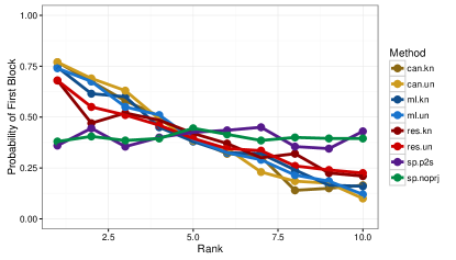
(a) Small scale simulation results

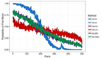
(b) Medium scale simulation results

Figure 1: The mean nomination lists for the (a) small and (b) medium stochastic block model experiments for the different vertex nomination techniques in both the known (dark colors) and unknown (light colors). Plot (a) shows performance for the canonical (gold), maximum likelihood (blue), restricted-focus maximum likelihood (red) and spectral (green and purple) methods. Spectral VN both with and without projection to the sphere is shown in purple and green, respectively. Plot (b) does not include canonical vertex nomination due to runtime constraints.

A more quantitative assessment of the vertex nomination methods is contained in Tables 1 and 2, which compare the performance of the methods as assessed by, respectively, average precision (AP) and adjusted Rand index (ARI). As defined in Equation (1), AP is a value between 0 and 1, where a value of 1 indicates perfect performance. ARI (Hubert and Arabie, 1985) measures how well a given partition of a set recovers some ground truth partition. Here a value of 1 indicates perfect recovery, while randomly partitioning a data set yields ARI approximately 0 (note that negative ARI is possible). We include ARI as an evaluation to highlight the fact that spectral and maximum likelihood vertex nomination do not merely classify vertices as interesting or not. Rather, they return a partition of the vertices into clusters. Canonical vertex nomination, on the other hand, makes no attempt to recover the full cluster structure of the graph, instead only attempting to classify vertices according to whether or not they are of interest. As such, we do not include ARI numbers for canonical vertex nomination. Turning first to performance in the small graph condition in Table 1, we see that $\mathcal{L}^{\operatorname{C}}$ is the best method, so long as the graph in question is small enough that the canonical method is tractable, but $\mathcal{L}^{\operatorname{ML}}$, regardless of whether or not model parameters are known, nearly matches canonical VN, and, unlike its canonical counterpart, scales to graphs with more than a few nodes. The numbers for $\mathcal{L}^{\operatorname{SP}}$ bear out our observation above, that the small graphs contain too little information for spectral VN to act upon, and $\mathcal{L}^{\operatorname{SP}}$ performs approximately at chance, as a result. It is worth noting that while $\mathcal{L}^{\operatorname{ML}}_{R}$ does not match the performance of $\mathcal{L}^{\operatorname{ML}}$, presumably owing to the fact that the restricted-focus algorithm does not use all of the information present in the graph, it still outperforms spectral nomination, and lags $\mathcal{L}^{\operatorname{ML}}$ by less than 0.1 AP.

Turning our attention to the medium case, we see again that $\mathcal{L}^{\operatorname{ML}}$ and $\mathcal{L}^{\operatorname{ML}}_{R}$ remain largely impervious to whether model parameters are known or not, presumably a consequence of the use of smoothing—we’ll see in the sequel that estimation can be the difference between near-perfect performance and near-chance. With more vertices, we see that spectral improves above chance, leaving restricted ML slightly worse, but spectral still fails to match the performance of ML VN, even when model parameters are unknown.

In sum, these results suggest that different size graphs (and different modeling assumptions) call for different vertex nomination methods. In small graphs, regardless of whether or not model parameters are known, canonical vertex nomination is both tractable and quite effective. In medium graphs, maximum likelihood vertex nomination remains tractable and achieves impressively good nomination. Of course, for graphs with thousands of vertices, $\mathcal{L}^{\operatorname{ML}}$ becomes computationally expensive, leaving only $\mathcal{L}^{\operatorname{SP}}$ and $\mathcal{L}^{\operatorname{ML}}_{R}$ as options. We have observed that $\mathcal{L}^{\operatorname{ML}}_{R}$ tends to lag $\mathcal{L}^{\operatorname{SP}}$ in such large graphs, though increasing the number of seeds (and hence the amount of information available to $\mathcal{L}^{\operatorname{ML}}_{R}$) closes this gap considerably. We leave for future work a more thorough exploration of under what circumstances we might expect $\mathcal{L}^{\operatorname{ML}}_{R}$ to be competitive with $\mathcal{L}^{\operatorname{SP}}$ in graphs on thousands of vertices.

	Known				Unknown
	ML	RES	SP	CAN	ML	RES	SP	CAN
small	0.670	0.588	0.388	0.700	0.680	0.606	0.415	0.710
medium	0.954	0.545	0.738	–	0.954	0.537	0.735	–

Table 1: Empirical estimates of mean average precision on the two stochastic block model data sets for the four methods under consideration. Each data point is the mean of 200 independent trials.

	Known				Unknown
	ML	RES	SP	CAN	ML	RES	SP	CAN
small	0.338	0.259	0.011	–	0.338	0.259	0.011	–
medium	0.572	0.039	0.268	–	0.572	0.037	0.271	–

Table 2: ARI on the different sized data sets for the ML, restricted ML, and spectral methods. Each data point is the mean of 200 independent trials. Performance of canonical vertex nomination is knot included, since canonical vertex nomination makes no attempt to recover all three blocks, and thus ARI is not a sensible measure.

6.2 Word Co-occurrences

We consider a linguistic data set consisting of co-occurrences of 54 nouns and 58 adjectives in Charles Dickens’ novel David Copperfield (Newman, 2006a). We construct a graph in which each node corresponds to a word, and an edge connects two nodes if the two corresponding words occurred adjacent to one another in the text. The adjacency matrix of this graph is shown in Figure 2. Visual inspection reveals a clear block structure, and that this block structure is clearly not assortative (i.e., inter-block edges are more frequent than intra-block edges). This runs contrary to many commonly-studied data sets and model assumptions. Figure 3 shows the performance of spectral and maximum-likelihood vertex nomination, measured by (a) average precision and adjusted Rand index (ARI) at various numbers of seeds. Each data point is the average over 1000 trials. In each trial, a set of $m$ seeds was chosen uniformly at random from the 112 nodes, with the restriction that at least one noun and one adjective be included in the seed set. Performance was then measured as the mean average precision in identifying the adjective block.

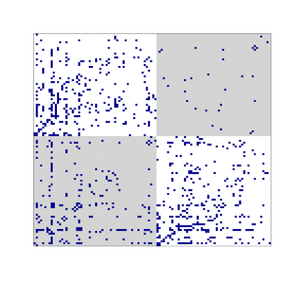
Figure 2: Adjacency matrix of the linguistic data set, arranged to highlight the graph’s structure. The grey shading indicates the two blocks, with adjectives in the lower left and nouns in the upper right. Note the disassortative block structure.

Figure 3 shows the performance of the VN schemes under consideration, as a function of the number of seed vertices, using both known (dark colors) and estimated (light colors) model parameters. Looking first at AP in Figure 3 (a), we see that ML in the known-parameter case (dark blue) does consistently well, even with only a handful of seeds, and attains near-perfect performance for $m\geq 20$. When model parameters must be estimated (light blue), ML is less dominant, thought it still performs nearly perfectly for $m\geq 20$. We note the dip in unknown-parameters ML as $m$ increases from $2$ to $5$ to $10$, a phenomenon we attribute to the bias-variance tradeoff. Namely, with more seeds available, variance in the estimated model parameters increases, but for $m<20$, this increase in variance is not offset by an appreciable improvement in estimation, possibly attributable to our use of add-one smoothing. Somewhat surprisingly, restricted-focus ML performs quite well, consistently improving on spectral VN in the known parameter case for $m>2$, and in the unknown parameter case once $m>10$. Finally, we turn our attention to spectral VN, shown in green for the variant in which we project embeddings to the sphere and in purple for the variant in which we do not. In contrast to our simulations, the sparsity of this network makes projection to the sphere a critical requirement for successful retrieval of the first block. Without projection to the sphere, spectral VN fails to rise appreciably above chance performance.

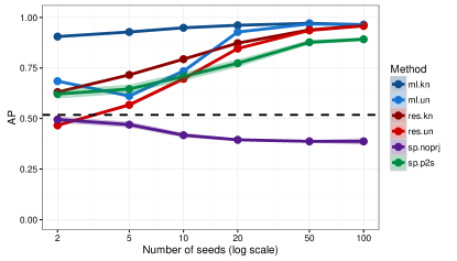
(a)

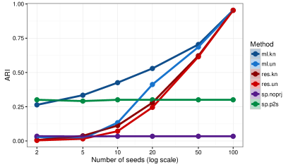
(b)

Figure 3: Performance on the linguistic data set as measured by (a) AP and (b) ARI as a function of the number of seeds for the ML vertex nomination (blue), restricted-focus ML (red), and spectral vertex nomination with (green) and without projection to the sphere (violet), when model parameters are known (light colors) and unknown (dark colors). Each data point is the mean of 1000 Monte Carlo trials, and shaded regions indicate two standard deviations of the mean.

6.3 Zachary’s Karate Club

We consider the classic sociological data set, Zachary’s karate club network (Zachary, 1977). The graph, visualized in Figure 4, consists of 34 nodes, each corresponding to a member of a college karate club, with edges joining pairs of club members according to whether or not those members were observed to interact consistently outside of the club. Over the course of Zachary’s observation of the group, a conflict emerged that led to the formation of two factions, led by the individuals numbered 1 and 34 in Figure 4, and these two factions constitute the two blocks in this experiment. Zachary’s karate data set is particularly well-suited for spectral methods. Indeed, the flow-based model originally proposed by Zachary recovers factions nearly perfectly, and visual inspection of the graph (Figure 4) suggests a natural cut separating the two factions. As such, we expect ML-based vertex nomination to lose out against the spectral-based method. Figure 5 shows performance of the two algorithms as measured by ARI and average precision. We see, as expected, that spectral performance performs nearly perfectly, irrespective of the number of seeds. Surprisingly, maximum likelihood nomination is largely competitive with spectral VN, but only provided that the model parameters are already known. Interesting to note that here again we see the phenomenon discussed previously in which ML performance with an unknown edge probability matrix degrades when going from $s=2$ seeds to $s=5$ before improving again, with AP comparable to the known case for $s\geq 20$.

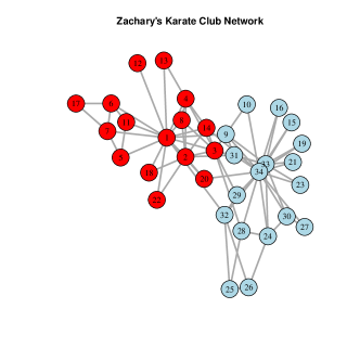
Figure 4: Visualization of the graph corresponding to Zachary’s karate club data set. The vertices are colored according to which of the two clubs each member chose to join after the schism. Our block of interest is in red.

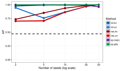
(a)

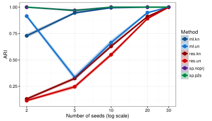
(b)

Figure 5: Performance on the karate data set as a function of the number of seeds for the ML vertex nomination (blue), restricted-focus ML nomination (red), and spectral vertex nomination with (green) and without projection to the sphere (violet), when model parameters are known (light colors) and unknown (dark colors), as measured by (a) AP and (b) ARI. The black dashed line indicates chance performance. Each observation is the mean of 1000 independent trials, with the shaded bars indicating two standard errors of the mean in either direction.

6.4 Political Blogs

We consider a network of American political blogs in the lead-up to the 2004 election (Adamic and Glance, 2005), where an edge joins two blogs if one links to the other, with blogs classified according to political leaning (liberal vs conservative). From an initial 1490 vertices, we removed all isolated vertices to obtain a network of 1224 vertices and 16718 edges. Figure 6 shows the performance of the spectral- and ML-based methods in recovering the liberal block. We observe first and foremost that the sparsity of this network results in exceptionally poor performance in both AP and ARI for spectral VN unless the embeddings are projected to the sphere, but that spectral vertex nomination is otherwise quite effective at recovering the liberal block, with performance nearly perfect for $m>10$. Unsurprisingly, ML and its restricted counterpart both perform approximately at-chance when $m<10$. We see that in both the known and unknown cases, ML VN is competitive with spectral VN for suitably large $m$ ($m\geq 50$ for known, $m\geq 500$ for unknown). As expected in such a sparse network, restricted-focus ML lags ML VN in the known-parameter case, but surprisingly, in the unknown-parameter case, restricted ML achieves remarkably better AP than does ML, a fact we are unable to account for, though it is worth noting that looking at ARI in Figure 6 (b), no such gap appears between ML and its restricted-focus counterpart in the unknown-parameter case.

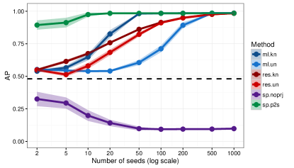
(a)

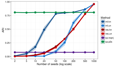
(b)

Figure 6: Performance on the political blogs data set as a function of the number of seeds for the ML vertex nomination (blue), restricted-focus ML (red), and spectral vertex nomination with (green) and without projection to the sphere (violet), when model parameters are known (light colors) and unknown (dark colors), as measured by (a) AP and (b) ARI.

6.5 Ecological Network

We consider a trophic network, consisting of 125 nodes and 1907 edges, in which nodes correspond to (groups of) organisms in the Florida Bay ecosystem (Ulanowicz et al., 1997; Nooy et al., 2011), and an edge joins a pair of organisms if one feeds on the other. Our features are the (log) mass of organisms. We take our community of interest to be the 16 different types of birds in the ecosystem. This choice makes for an interesting task for several reasons. Firstly, unlike the other data sets we consider, our community of interest is a comparatively small fraction of the network—it consists of a mere 16 nodes of 125 in total. Further, our block of interest is comparatively heterogeneous in the sense that the roles of the different types of birds in the Florida Bay ecosystem is quite diverse. For example, the block of interest includes both raptors and shorebirds, which feed on quite different collections of organisms. Finally, it stands to reason that the mass of the organisms in question might be a crucial piece of information for disambiguating, say, a raptor from a shark. Thus, we expect that using node features will be crucial for retrieving the block of interest.

The topology of the Florida Bay network is shown in Figure 7 (a). Note that the block of interest, indicated in red, has a strongly disassortative structure. Indeed, all intra-block edges in the red block are incident to the node corresponding to raptors. Figure 7 (b) summarizes vertex nomination performance for several methods. The plot shows performance, as measured by mean average precision (AP), as a function of the number of seeds for several different nomination schemes. As in earlier plots, dark colors correspond to model parameters being known, while light colors correspond to model parameters being estimated using the seed vertices. We see immediately that spectral nomination (green and purple) and ML VN (blue) fail to improve appreciably upon chance performance except when the vast majority of the vertices’ labels are observed. Like in the linguistic data set presented above, the disassortative structure of the data appears to cause problems for spectral nomination. The failure of ML suggests that no useful information is encoded in the graph itself, but turning our attention to the curves corresponding to $\mathcal{L}^{\operatorname{ML}}_{F}$ (red) and using only features (gold), we see that this is not the case. Indeed, we see that while using features alone achieves a marked improvement over both spectral and ML-based nomination, using both features and graph matching in the form of $\mathcal{L}^{\operatorname{ML}}_{F}$ yields an additional improvement of some 0.1 AP in the range of $m=8,16,32$. This result suggests that there may be cases where the only reliable way to retrieve vertices of interest is to leverage both features and graph topology jointly.

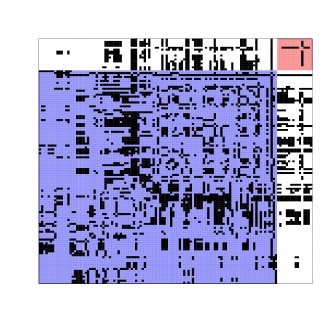
(a)

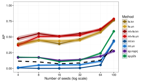
(b)

Figure 7: (a) The adjacency matrix of the Florida Bay trophic network. Nodes correspond to classes of plants and animals (e.g., sharks, rays, shorebirds, zooplankton, phytoplankton). An edge joins two nodes if the corresponding organisms are in a predator-prey relation. The sixteen types of birds in the network are highlighted in the red block. Note the disassortative structure of the bird block (the edges within the red block are all incident to the node that corresponds to raptors).  (b) Average precision in identifying the bird nodes as a function of the number of seed vertices for ML vertex nomination (blue), restricted-focus ML (red), and spectral vertex nomination with (green) and without projection to the sphere (violet), when model parameters are known (light colors) and unknown (dark colors). The black dashed line indicates chance performance.

7 Discussion and Future Work

Network data has become ubiquitous in the sciences, giving rise to a vast array of computational and statistical problems that are only beginning to be explored. In this paper, we have explored one such problem that arises when working with network data, namely the task of performing vertex nomination. This task, in some sense the graph analogue of the classic information retrieval problem, is fundamental to exploratory data analysis on graphs as well as to machine learning applications. Above, we established the consistency of two methods of vertex nomination: a maximum-likelihood scheme $\mathcal{L}^{\operatorname{ML}}$ and its restricted-focus variant $\mathcal{L}^{\operatorname{ML}}_{R}$, in which we obtain a feasibly exactly-solvable optimization problem at the expense of using less than the full information available in the graph. Additionally, we have introduced a maximum-likelihood vertex nomination scheme for the case where vertices are endowed with features and when (possibly weighted) edges are drawn from a canonical exponential family. The key to all of these methods is the ability to quickly approximate a solution to the seeded graph matching problem.

We have presented experimental comparisons of these methods against each other and against several other benchmark methods, where we see that the best choice of method depends highly on graph size and structure. The major tradeoff appears to be that large graphs (tens of thousands of vertices) are not tractable for $\mathcal{L}^{\operatorname{ML}}$, but in smaller and medium-sized graphs, $\mathcal{L}^{\operatorname{ML}}$ can detect signal where spectral methods fail to do so. It is worth noting that $\mathcal{L}^{\operatorname{ML}}$, and, to a lesser extent, $\mathcal{L}^{\operatorname{ML}}_{R}$, is quite competitive with $\mathcal{L}^{\operatorname{SP}}$, and even manages to best $\mathcal{L}^{\operatorname{SP}}$ when the structure of the graph is ill-suited to the typical assumptions of spectral methods, as in the case of our linguistic data set. All told, our experimental results mirror those in Fishkind et al. (2015) and point toward a theory of which methods are best-suited to which graphs, a direction that warrants further exploration.

Appendix A Proof Details

Before proving Theorem 6, we first state a useful initial proposition.

Proposition 12.

Let $\vec{x}=(x_{1},x_{2},\ldots,x_{k})$ be a vector with distinct entries in $\mathbb{R}^{k}$. Let $f(\cdot)$ be a strictly increasing real valued function (with the abuse of notation, $f(\vec{x}$), denoting $f(\cdot)$ applied entrywise to $\vec{x}$). Let the order statistics of $\vec{x}$ be denoted

$$x_{(1)}<x_{(2)}<\cdots<x_{(k)},$$

and define $\alpha=\min_{i\in\{2,3,\ldots,k\}}|x_{(i)}-x_{(i-1)}|$, and $\beta=\min_{i\in\{2,3,\ldots,k\}}|f(x_{(i)})-f(x_{(i-1)})|$. If $\sigma$ is the cyclic permutation

$$\sigma=\begin{pmatrix}1&2&3&\cdots&k\\ 2&3&4&\cdots&1\end{pmatrix},$$

then

$$\langle\vec{x},f(\vec{x})\rangle-\langle\vec{x},f(\sigma(\vec{x}))\rangle\geq(k-1)\alpha\beta.$$

Proof.

We will induct on $k$. To establish the base case, $k=2$, let $x_{1}=x_{(1)}$ without loss of generality and observe that

$$\langle\vec{x},f(\vec{x})\rangle-\langle\vec{x},f(\sigma(\vec{x}))\rangle =(x_{2}-x_{1})(f(x_{2})-f(x_{1}))$$

$$=(x_{(2)}-x_{(1)})(f(x_{(2)})-f(x_{(1)}))\geq\alpha\beta.$$

For general $k$, again, without loss of generality let $x_{1}=x_{(1)}$, and define the permutation

$$\tau=\begin{pmatrix}2&3&\cdots&k\\ 3&4&\cdots&2\end{pmatrix}.$$

Then

$$\langle\vec{x},f(\vec{x})\rangle-\langle\vec{x},f(\sigma(\vec{x}))\rangle =\langle\vec{x},f(\vec{x})\rangle-\langle\vec{x},f(\tau(\vec{x}))\rangle+\langle\vec{x},f(\tau(\vec{x}))\rangle-\langle\vec{x},f(\sigma(\vec{x}))\rangle$$

$$=\langle\vec{x},f(\vec{x})\rangle-\langle\vec{x},f(\tau(\vec{x}))\rangle+(x_{k}-x_{1})(f(x_{2})-f(x_{1}))$$

$$\geq\langle\vec{x},f(\vec{x})\rangle-\langle\vec{x},f(\tau(\vec{x}))\rangle+\alpha\beta,$$

and the result follows from the inductive hypothesis. ∎

Remark 13.

It follows immediately that in Proposition 12, if there exists an index $i\in[k]$ such that $\alpha_{i}=\min_{j\neq i}|x_{(i)}-x_{(j)}|>0$, and $\beta_{i}=\min_{j\neq i}|f(x_{(i)})-f(x_{(j)})|>0$, then $\langle\vec{x},f(\vec{x})\rangle-\langle\vec{x},f(\sigma(\vec{x}))\rangle\geq\alpha_{i}\beta_{i}.$

We are now ready to prove Theorem 6.

Proof of Theorem 6.

Define

$$X_{P}:=\operatorname{tr}(AB^{\top})-\operatorname{tr}(A(I_{m}\oplus P)B(I_{m}\oplus P)^{\top})$$

and define $\mathcal{P}=\{P\in\Pi_{\mathfrak{u}}:\epsilon_{1,\bullet}(P)>0\}$. We will show that

$$\mathbb{P}\left(\exists\,\,P\in\mathcal{P}\text{ s.t. }X_{P}\leq 0\right)=O(1/n^{2}),$$

from which the desired consistency of $\mathcal{L}^{\operatorname{ML}}$ follows by the Borel-Cantelli Lemma, since this probability is summable in $n$. Fix $P\in\mathcal{P}$, and let $\sigma_{P}\in S_{n}$ be the permutation associated with $I_{m}\oplus P$. The action of shuffling $B$ via $I_{m}\oplus P$ is equivalent to permuting the $[n^{2}]$ elements of $\text{vec}(B)$ via a permutation $\tau_{P}$, in that

$$\operatorname{tr}(A(I_{m}\oplus P)B(I_{m}\oplus P)^{\top})=\langle\text{vec}(A),\tau_{P}(\text{vec}(B))\rangle.$$

Moreover, $\tau_{P}$ can be chosen so that, in the cyclic decomposition of $\tau_{P}=\tau_{P}^{(1)}\tau_{P}^{(2)}\cdots\tau_{P}^{(\ell)}$, each (disjoint) cycle is acting on a set of distinct real numbers. Note that Proposition 12 implies that the contribution of each cycle $\tau_{P}^{(i)}$ to $\mathbb{E}(X_{P})$ is nonnegative, and the assumptions of Theorem 6 imply that for each $i,j\in[K]$ such that $i\neq j$, the contribution of each (nontrivial) cycle permuting a $\Lambda_{i,i}$ entry to a $\Lambda_{i,j}$ entry contributes at least $\alpha\beta$ to $\mathbb{E}(X_{P})$. It follows immediately that

$$\mathbb{E}(X_{P}) =\mathbb{E}\left(\operatorname{tr}(AB)-\operatorname{tr}(APBP^{\top})\right)$$

$$=\mathbb{E}\left(\langle\text{vec}(A),\text{vec}(B)\rangle-\langle\text{vec}(A),\tau_{P}(\text{vec}(B)\rangle\right)$$

$$\geq 2\alpha\beta\sum_{i}\left(\frac{1}{2}\sum_{j}\sum_{k\neq j}\epsilon_{i,j}\epsilon_{i,k}+m_{i}\epsilon_{i,\bullet}\right)$$

$$\geq 2\alpha\beta\sum_{i}\left(\frac{(\mathfrak{u}_{i}-\epsilon_{i,\bullet})\epsilon_{i,\bullet}}{2}+m_{i}\epsilon_{i,\bullet}\right).$$

Let $\mathfrak{n}(P)$ be the total number of distinct entries of vec$(B)$ permuted by $\tau_{P}$, and note that an application of Proposition 12 yields

$$\mathbb{E}(X_{P}) =\mathbb{E}\left(\operatorname{tr}(AB)-\operatorname{tr}(APBP^{\top})\right)$$

$$=\mathbb{E}\left(\langle\text{vec}(A),\text{vec}(B)\rangle-\langle\text{vec}(A),\tau_{P}(\text{vec}(B)\rangle\right)$$

$$\geq\frac{1}{2}\mathfrak{n}(P)\gamma\kappa.$$

The assumptions in the Theorem also immediately yield that

$$\mathfrak{n}(P)\geq\sum_{k}\left(\frac{(\mathfrak{u}_{k}-\epsilon_{k,\bullet})\epsilon_{k,\bullet}}{2}+m_{k}\epsilon_{k,\bullet}\right).$$

We next note that $X_{P}$ is a sum of $\mathfrak{n}(P)$ independent random variables, each bounded in $[-c,c]$. An application of Hoeffding’s inequality then yields

$$\mathbb{P}(X_{P}\leq 0) \leq\mathbb{P}\left(|X_{P}-\mathbb{E}X_{P}|\geq\mathbb{E}X_{P}\right)\leq 2\exp\left\{-\frac{2\mathbb{E}^{2}X_{P}}{4c^{2}\mathfrak{n}(P)}\right\}$$

$$\leq 2\exp\left\{-\frac{|\mathbb{E}X_{P}|\kappa\gamma}{2c^{2}}\right\}\leq 2\exp\left\{-\frac{\alpha\beta\kappa\gamma}{4c^{2}}\sum_{k}\left(\frac{(\mathfrak{u}_{k}-\epsilon_{k,\bullet})\epsilon_{k,\bullet}}{2}+m_{k}\epsilon_{k,\bullet}\right)\right\}.$$

Next, note that

$$|\{P\in\mathcal{P}\text{ s.t. }X_{P}\leq 0\}|=0\text{ iff }|\{P\in\mathcal{P}/\sim\text{ s.t. }X_{P}\leq 0\}|=0.$$

Given $\{\epsilon_{k,\ell}\}_{k,\ell=1}^{K}$ satisfying $\mathfrak{u}_{k}=\sum_{\ell}\epsilon_{k,\ell}=\sum_{\ell}\epsilon_{\ell,k}$ for all $k\in[K]$, the number of elements $P\in\mathcal{P}/\sim$ with $\epsilon_{k,\ell}(P)=\epsilon_{k,\ell}$ for all $k,\ell\in[K]$ is at most

$$\mathfrak{u}_{1}^{\sum_{\ell\neq 1}\epsilon_{1,\ell}}\mathfrak{u}_{2}^{\sum_{\ell\neq 2}\epsilon_{2,\ell}}\cdots\mathfrak{u}_{K}^{\sum_{\ell\neq K}\epsilon_{K,\ell}} =\mathfrak{u}_{1}^{\mathfrak{u}_{1}-\epsilon_{1,1}}\mathfrak{u}_{2}^{\mathfrak{u}_{2}-\epsilon_{2,2}}\cdots\mathfrak{u}_{K}^{\mathfrak{u}_{K}-\epsilon_{K,K}}$$

$$=e^{\sum_{k}(\mathfrak{u}_{k}-\epsilon_{k,k})\log(\mathfrak{u}_{k})}.$$ (12)

The number of ways to choose such a set (i.e. the $\{\epsilon_{k,\ell}\}_{k,\ell}^{K}$) is bounded above by

$$\prod_{\begin{subarray}{c}k\text{ s.t. }\epsilon_{k,\bullet}\neq 0\end{subarray}}(\mathfrak{u}_{k}+K)^{K}=e^{\sum_{\begin{subarray}{c}k\text{ s.t. }\epsilon_{k,\bullet}\neq 0\end{subarray}}K\log(\mathfrak{u}_{k}+K)}.$$ (13)

Applying the union bound over all $P\in\mathcal{P}/\sim$, we then have

$$\mathbb{P}\big{(}\,\exists\,P\in\mathcal{P}\text{ s.t. }X_{P}\leq 0\,\big{)}=\mathbb{P}\big{(}\,\exists\,P\in\mathcal{P}/\sim\text{ s.t. }X_{P}\leq 0\,\big{)}$$

$$\leq\exp\bigg{\{}-\frac{\alpha\beta\kappa\gamma}{2c^{2}}\sum_{k}\left(\frac{(\mathfrak{u}_{k}-\epsilon_{k,\bullet})\epsilon_{k,\bullet}}{2}+m_{k}\epsilon_{k,\bullet}\right)$$ (14)

$$\hskip 45.5244pt+\sum_{k}(\mathfrak{u}_{k}-\epsilon_{k,k})\log\mathfrak{u}_{k}+\!\!\!\!\!\sum_{\begin{subarray}{c}k\text{ s.t. }\epsilon_{k,\bullet}\neq 0\end{subarray}}\!\!\!\!\!\!K\log(\mathfrak{u}_{k}+K)\bigg{\}}.$$ (15)

It remains for us to establish that the expression inside the exponent goes to $-\infty$ fast enough to ensure our desired bound. For each $k$, the contribution to the exponent in (A) is

$$-\frac{\alpha\beta\kappa\gamma}{2c^{2}}\left(\frac{(\mathfrak{u}_{k}-\epsilon_{k,\bullet})\epsilon_{k,\bullet}}{2}+m_{k}\epsilon_{k,\bullet}\right)+(\mathfrak{u}_{k}-\epsilon_{k,k})\log\mathfrak{u}_{k}+\mathbbm{1}\{\epsilon_{k,\bullet}\neq 0\}K\log(\mathfrak{u}_{k}+K)$$

$$=-\frac{\alpha\beta\kappa\gamma}{2c^{2}}\left(\frac{\epsilon_{k,k}\epsilon_{k,\bullet}}{2}+m_{k}\epsilon_{k,\bullet}\right)+\epsilon_{k,\bullet}\log\mathfrak{u}_{k}+\mathbbm{1}\{\epsilon_{k,\bullet}\neq 0\}K\log(\mathfrak{u}_{k}+K)$$ (16)

If $\mathfrak{u}_{k}/2\leq\epsilon_{k,k}<\mathfrak{u}_{k}$, then

$$\epsilon_{k,k}\epsilon_{k,\bullet}\geq\frac{\mathfrak{u}_{k}\epsilon_{k,\bullet}}{2}=\omega(\epsilon_{k,\bullet}\log\mathfrak{u}_{k}),\text{ and }\epsilon_{k,k}\epsilon_{k,\bullet}\geq\frac{\mathfrak{u}_{k}\epsilon_{k,\bullet}}{2}=\omega(K\log(\mathfrak{u}_{k}+K)),$$

and the contribution to the exponent in (A) from $k$, Eq. (A), is clearly bounded above by $-2\log(n)$ for sufficiently large $n$. If $\epsilon_{k,k}\leq\mathfrak{u}_{k}/2$ then $\epsilon_{k,\bullet}>\mathfrak{u}_{k}/2$, and

$$m_{k}\epsilon_{k,\bullet}=\omega(\epsilon_{k,\bullet}\log\mathfrak{u}_{k}),\text{ and }m_{k}\epsilon_{k,\bullet}\geq\frac{m_{k}\mathfrak{u}_{k}}{2}=\omega(K\log(\mathfrak{u}_{k}+K)),$$

and the contribution to the exponent in (A) from $k$, Eq. (A), is clearly bounded above by $-2\log(n)$ for sufficiently large $n$. If $\epsilon_{k,k}=\mathfrak{u}_{k}$, then all terms in the exponent (A) are equal to $0$. For sufficiently large $n$, Eq. (A) is then bounded above by

$$\exp\left\{-\!\!\!\!\!\sum_{\begin{subarray}{c}k\text{ s.t. }\epsilon_{k,\bullet}\neq 0\end{subarray}}\!\!\!\!\!\!2\log(n)\right\}\leq\exp\left\{-2\log(n)\right\},$$

and the result follows. ∎

Consistency of $\mathcal{L}^{\operatorname{ML}}_{R}$ as claimed in Theorem 8 follows similarly to that of $\mathcal{L}^{\operatorname{ML}}$, and we next briefly sketch the details of the proof.

Proof of Theorem 8 (Sketch).

Analogously to the proof of Theorem 6, define

$$X_{P}:=\operatorname{tr}\left((A^{(1,2)})^{\top}B^{(1,2)}\right)-\operatorname{tr}\left((A^{(1,2)})^{\top}B^{(1,2)}P^{\top}\right).$$

The proof follows mutatis mutandis to the proof of Theorem 6, with the key difference being that in this case,

$$\mathbb{E}(X_{P}) =\mathbb{E}\left(\operatorname{tr}\left((A^{(1,2)})^{\top}B^{(1,2)}\right)-\operatorname{tr}\left((A^{(1,2)})^{\top}B^{(1,2)}P^{\top}\right)\right)$$

$$\geq 2\alpha\beta\sum_{k}m_{k}\epsilon_{k,\bullet}.$$

Details are omitted for brevity. ∎

Before proving Theorem 9 we establish some preliminary concentration results for our estimates $\widehat{\Lambda}$, and $\hat{n}_{k}$, $k\in[K]$. An application of Hoeffding’s inequality yields that for $k,\ell\in[K]$ such that $k\neq\ell$,

$$\mathbb{P}\left(\left|\widehat{\Lambda}_{k,\ell}-\Lambda_{k,\ell}\right|\geq\frac{\sqrt{n\log n}}{m_{k}m_{\ell}}\right)\leq 2\text{exp}\left\{-2n\log n\right\},$$ (17)

and for $k\in[K]$,

$$\mathbb{P}\left(\left|\widehat{\Lambda}_{k,k}-\Lambda_{k,k}\right|\geq\frac{\sqrt{n\log n}}{\binom{m_{k}}{2}}\right)\leq 2\text{exp}\left\{-2n\log n\right\},$$ (18)

and

$$\mathbb{P}\left(\left|\hat{n}_{k}-n_{k}\right|\geq t\right)\leq 2\text{exp}\left\{\frac{-2mt^{2}}{n^{2}}\right\},$$ (19)

With $\gamma$ defined as in (8), define the events $\mathcal{E}^{(1)}_{n}$ and $\mathcal{E}^{(2)}_{n}$ via

$$\mathcal{E}^{(1)}_{n}=\left\{\forall\,\,\{k,\ell\}\in\binom{[K]}{2},\text{ s.t }|\Lambda_{k,k}-\Lambda_{k,\ell}|>\gamma,\text{ it holds that }\left|\widehat{\Lambda}_{k,k}-\widehat{\Lambda}_{k,\ell}\right|>\frac{\gamma}{2}\right\};$$

$$\mathcal{E}^{(2)}_{n}=\left\{\forall\,\,k\in[K],\,|\hat{n}_{k}-n_{k}|\leq n_{k}^{2/3}\right\}.$$

Combining (17)–(19), we see that if for each $k\in[K]$, $n_{k}=\Theta(n)$, $\min_{k}m_{k}=\omega(\sqrt{n_{k}}\log(n_{k}))$, then for sufficiently large $n$,

$$\mathbb{P}\left((\mathcal{E}^{(1)}_{n}\cup\mathcal{E}^{(2)}_{n})^{c}\right)\leq e^{-2\log n}.$$ (20)

We are now ready to prove Theorem 9, proving the consistency of $\mathcal{L}^{\operatorname{ML}}$ when the model parameters are unknown.

Proof of Theorem 9.

Let $\widehat{B}$ be our estimate of $B$ using the seed vertices; i.e., there are $\hat{n}_{k}$ vertices from block $k$ for each $k\in[K]$, and for each $k,\ell\in[K]$, the entry of $\widehat{B}$ between a block $k$ vertex and a block $\ell$ vertex is

$$\log\left(\frac{\widehat{\Lambda}_{k,\ell}}{1-\widehat{\Lambda}_{k,\ell}}\right).$$

Let $\widehat{L}$ be the set of distinct entries of $\widehat{\Lambda}$, and define

$$\hat{\alpha}=\min_{\{k,\ell\}\text{ s.t. }k\neq\ell}|\widehat{\Lambda}_{k,k}-\widehat{\Lambda}_{k,\ell}|\hskip 14.22636pt\hat{\beta}=\min_{\{k,\ell\}\text{ s.t. }k\neq\ell}|\widehat{B}_{k,k}-B_{k,\ell}|\hskip 14.22636pt\hat{c}=\max_{i,j,k,\ell}|\widehat{B}_{i,j}-\widehat{B}_{k,\ell}|,$$ (21)

$$\hskip 56.9055pt\hat{\gamma}=\min_{x,y\in\widehat{L}}|x-y|,\hskip 14.22636pt\hat{\kappa}=\min_{x,y\in\widehat{L}}\left|\log\left(\frac{x}{1-x}\right)-\log\left(\frac{y}{1-y}\right)\right|.$$ (22)

Note that conditioning on $\mathcal{E}^{(1)}_{n}\cup\mathcal{E}^{(2)}_{n}$ and assumption iv. ensures that each of $\hat{\alpha}$, $\hat{\beta}$, $\hat{c}$, $\hat{\gamma}$, and $\hat{\kappa}$ is bounded away from $0$ by an absolute constant for sufficiently large $n$. For each $k\in[K],$ define

$$\mathfrak{e}_{k}:=|\hat{n}_{k}-n_{k}|=|\mathfrak{\hat{u}}_{k}-\mathfrak{u}_{k}|,\hskip 14.22636pt\mathfrak{e}=\sum_{k}\mathfrak{e}_{k},\hskip 14.22636pt\eta_{k}:=\min(n_{k},\hat{n}_{k}),\hskip 14.22636pt\eta=\sum_{k}\eta_{k},$$ (23)

and note that conditioning on $\mathcal{E}^{(1)}_{n}\cup\mathcal{E}^{(2)}_{n}$ ensures that $\mathfrak{e}_{k}=O(n_{k}^{2/3})$ for all $k\in[K].$ An immediate result of this is that, conditioning on $\mathcal{E}^{(1)}_{n}\cup\mathcal{E}^{(2)}_{n}$, we have that $\eta_{k}=\Theta(n_{k})=\Theta(n)$ for all $k\in[K]$.

Define $\mathcal{P}:=\{P\in\Pi_{\mathfrak{u}}:\epsilon_{1,\bullet}(P)>n^{2/3}\log n\}$, and for $P\in\Pi_{\mathfrak{u}}$, define

$$X_{P}:=\operatorname{tr}(A\tilde{B}^{\top})-\operatorname{tr}(A(I_{m}\oplus P)\tilde{B}(I_{m}\oplus P)^{\top}).$$

We will show that

$$\mathbb{P}\left(\exists\,\,P\in\mathcal{P}\text{ s.t. }X_{P}\leq 0\right)=O(1/n^{2}),$$

and the desired consistency of $\mathcal{L}^{\operatorname{ML}}$ follows immediately. To this end, decompose $A$ and $B$ as

$$A=\hbox{}\vbox{\kern 0.86108pt\hbox{$\kern 0.0pt\kern 2.5pt\kern-5.0pt\left[\kern 0.0pt\kern-2.5pt\kern-5.55557pt\vbox{\kern-0.86108pt\vbox{\vbox{ \halign{\kern\arraycolsep\hfil\@arstrut$\kbcolstyle#$\hfil\kern\arraycolsep& \kern\arraycolsep\hfil$\@kbrowstyle#$\ifkbalignright\relax\else\hfil\fi\kern\arraycolsep&& \kern\arraycolsep\hfil$\@kbrowstyle#$\ifkbalignright\relax\else\hfil\fi\kern\arraycolsep\cr 5.0pt\hfil\@arstrut$\scriptstyle$\hfil\kern 5.0pt&5.0pt\hfil$\scriptstyle\eta$\hfil\kern 5.0pt&5.0pt\hfil$\scriptstyle\mathfrak{e}\\\eta$\hfil\kern 5.0pt&5.0pt\hfil$\scriptstyle A^{(c,c)}$\hfil\kern 5.0pt&5.0pt\hfil$\scriptstyle A^{(c,e)}\\\mathfrak{e}$\hfil\kern 5.0pt&5.0pt\hfil$\scriptstyle A^{(e,c)}$\hfil\kern 5.0pt&5.0pt\hfil$\scriptstyle A^{(e,e)}$\hfil\kern 5.0pt\crcr}}}}\right]$}}\hskip 28.45274ptB=\hbox{}\vbox{\kern 0.86108pt\hbox{$\kern 0.0pt\kern 2.5pt\kern-5.0pt\left[\kern 0.0pt\kern-2.5pt\kern-5.55557pt\vbox{\kern-0.86108pt\vbox{\vbox{ \halign{\kern\arraycolsep\hfil\@arstrut$\kbcolstyle#$\hfil\kern\arraycolsep& \kern\arraycolsep\hfil$\@kbrowstyle#$\ifkbalignright\relax\else\hfil\fi\kern\arraycolsep&& \kern\arraycolsep\hfil$\@kbrowstyle#$\ifkbalignright\relax\else\hfil\fi\kern\arraycolsep\cr 5.0pt\hfil\@arstrut$\scriptstyle$\hfil\kern 5.0pt&5.0pt\hfil$\scriptstyle\eta$\hfil\kern 5.0pt&5.0pt\hfil$\scriptstyle\mathfrak{e}\\\eta$\hfil\kern 5.0pt&5.0pt\hfil$\scriptstyle B^{(c,c)}$\hfil\kern 5.0pt&5.0pt\hfil$\scriptstyle B^{(c,e)}\\\mathfrak{e}$\hfil\kern 5.0pt&5.0pt\hfil$\scriptstyle B^{(e,c)}$\hfil\kern 5.0pt&5.0pt\hfil$\scriptstyle B^{(e,e)}$\hfil\kern 5.0pt\crcr}}}}\right]$}},$$

where $A^{(c,c)}$ (resp., $B^{(c,c)}$) is an $\eta\times\eta$ submatrix of $A$ (resp., $B$)—which contains the seed vertices in $A$—with exactly $\eta_{k}$ vertices (resp., labels) from block $k$ for each $k\in[K]$. We view $A^{(c,c)}$ as the “core” matrix of $A$ (with $A^{(e,e)}$ and $A^{(c,e)}$ being the “errorful” part of $A$), as $A^{(c,c)}$ is a submatrix of $A$ that we could potentially cluster perfectly along block assignments. Note that similarly decomposing $P$ as

$$P=\hbox{}\vbox{\kern 0.86108pt\hbox{$\kern 0.0pt\kern 2.5pt\kern-5.0pt\left[\kern 0.0pt\kern-2.5pt\kern-5.55557pt\vbox{\kern-0.86108pt\vbox{\vbox{ \halign{\kern\arraycolsep\hfil\@arstrut$\kbcolstyle#$\hfil\kern\arraycolsep& \kern\arraycolsep\hfil$\@kbrowstyle#$\ifkbalignright\relax\else\hfil\fi\kern\arraycolsep&& \kern\arraycolsep\hfil$\@kbrowstyle#$\ifkbalignright\relax\else\hfil\fi\kern\arraycolsep\cr 5.0pt\hfil\@arstrut$\scriptstyle$\hfil\kern 5.0pt&5.0pt\hfil$\scriptstyle\eta$\hfil\kern 5.0pt&5.0pt\hfil$\scriptstyle\mathfrak{e}\\\eta$\hfil\kern 5.0pt&5.0pt\hfil$\scriptstyle P^{(c,c)}$\hfil\kern 5.0pt&5.0pt\hfil$\scriptstyle P^{(c,e)}\\\mathfrak{e}$\hfil\kern 5.0pt&5.0pt\hfil$\scriptstyle P^{(e,c)}$\hfil\kern 5.0pt&5.0pt\hfil$\scriptstyle P^{(e,e)}$\hfil\kern 5.0pt\crcr}}}}\right]$}},$$

we see that there exists a principal permutation submatrix of $P^{(c,c)}$ of size $(\eta-2\mathfrak{e})\times(\eta-2\mathfrak{e})$, which we denote $\tilde{P}$ (with associated permutation $\tilde{\sigma}$). This matrix represents a subgraph of the core vertices of $A$ mapped to a subgraph of the core vertices in $B$. We can then write $P=\tilde{P}\oplus Q,$ where $Q\in\Pi_{3\mathfrak{e}}.$ For each $k,\ell\in[K],$ let

$$\tilde{\epsilon}_{k,\ell}=\tilde{\epsilon}_{k,\ell}(\tilde{P})=|\{v\in U_{k}\text{ s.t. }\tilde{\sigma}(v)\in U_{k}\}|$$

Consider now

$$X_{P} =\operatorname{tr}(A(I_{\eta-3\mathfrak{e}}\oplus Q)B(I_{\eta-3\mathfrak{e}}\oplus Q)^{\top})-\operatorname{tr}(A(\tilde{P}\oplus Q)B(\tilde{P}\oplus Q)^{\top}).$$ (24)

Letting $\mathfrak{\tilde{u}}_{k}$ denote the number of vertices from the $k$-th block acted on by $\tilde{P}$, our assumptions yield

$$\mathbb{E}(X_{P})\geq 2\hat{\alpha}\hat{\beta}\sum_{k}\left(\frac{(\mathfrak{\tilde{u}}_{k}-\tilde{\epsilon}_{k,\bullet})\tilde{\epsilon}_{k,\bullet}}{2}+m_{k}\tilde{\epsilon}_{k,\bullet}\right)-\Theta(\eta\mathfrak{e})-\Theta(\mathfrak{e}^{2}).$$

Let $\mathfrak{\tilde{n}}(P)$ be the total number of distinct entries of vec$(B^{(c,c)})$ permuted by $\tilde{P}$, and note that another application of Proposition 12 yields

$$\mathbb{E}(X_{P})\geq\frac{1}{2}\mathfrak{\tilde{n}}(P)\hat{\gamma}\hat{\kappa}-\Theta(\eta\mathfrak{e})-\Theta(\mathfrak{e}^{2}).$$

The assumptions in the Theorem also immediately yield that

$$\mathfrak{\tilde{n}}(P)\geq\sum_{k}\left(\frac{(\mathfrak{\tilde{u}}_{k}-\tilde{\epsilon}_{k,\bullet})\tilde{\epsilon}_{k,\bullet}}{2}+m_{k}\tilde{\epsilon}_{k,\bullet}\right).$$

We then have that there exists a constants $c_{1}>0$ and $c_{2}>0$ such that

$$\mathbb{P}\big{(}\,\exists\,P\in\mathcal{P}\text{ s.t. }X_{P}\leq 0\,\big{|}\,\mathcal{E}^{(1)}_{n}\cup\mathcal{E}^{(2)}_{n}\big{)}=\mathbb{P}\big{(}\,\exists\,P\in\mathcal{P}/\sim\text{ s.t. }X_{P}\leq 0\,\big{|}\,\mathcal{E}^{(1)}_{n}\cup\mathcal{E}^{(2)}_{n}\big{)}$$

$$\leq\exp\bigg{\{}-\frac{\hat{\alpha}\hat{\beta}\hat{\kappa}\hat{\gamma}}{2\hat{c}^{2}}\sum_{k}\left(\frac{(\mathfrak{\tilde{u}}_{k}-\tilde{\epsilon}_{k,\bullet})\tilde{\epsilon}_{k,\bullet}}{2}+m_{k}\tilde{\epsilon}_{k,\bullet}\right)+\Theta(\eta\mathfrak{e})+\Theta(\mathfrak{e}^{2})$$

$$\hskip 45.5244pt+\sum_{k}(\mathfrak{\tilde{u}}_{k}-\tilde{\epsilon}_{k,k})\log\mathfrak{\tilde{u}}_{k}+~{}~{}~{}~{}\sum_{\begin{subarray}{c}k\text{ s.t. }\tilde{\epsilon}_{k,\bullet}\neq 0\end{subarray}}\!\!\!\!\!\!K\log(\mathfrak{\tilde{u}}_{k}+K)+O(\mathfrak{e}\log\mathfrak{e})\bigg{\}}$$

$$=\exp\bigg{\{}-c_{1}\sum_{k}\left(\frac{(\mathfrak{\tilde{u}}_{k}-\tilde{\epsilon}_{k,\bullet})\tilde{\epsilon}_{k,\bullet}}{2}+m_{k}\tilde{\epsilon}_{k,\bullet}\right)$$ (25)

$$\hskip 45.5244pt+\sum_{k}\tilde{\epsilon}_{k,\bullet}\log\mathfrak{\tilde{u}}_{k}+\!\!\!\!\sum_{\begin{subarray}{c}k\text{ s.t. }\tilde{\epsilon}_{k,\bullet}\neq 0\end{subarray}}\!\!\!\!\!\!K\log(\mathfrak{\tilde{u}}_{k}+K)+\Theta(n\mathfrak{e})\bigg{\}}$$

$$\leq\text{exp}\{-c_{2}n^{7/4}\log n\}.$$ (26)

Unconditioning Equation (A) combined with Equation (20) yields the desired result. ∎

Proof of Theorem 10 (Sketch).

The proof of Theorem 10 is a straightforward combination of the proofs of Theorems 8 and 9 once we have defined

$$\mathcal{P}:=\{P\in\Pi_{\mathfrak{u}}:\epsilon_{1,\bullet}(P)>n^{8/9}\log n\}.$$

Details are omitted for the sake of brevity. ∎

References

- Adamic and Glance [2005] L. A. Adamic and N. Glance. The political blogosphere and the 2004 US election. In Proc. WWW-2005 Workshop on the Weblogging Ecosystem, 2005.
- Airoldi et al. [2008] E. M. Airoldi, D. M. Blei, S. E. Fienberg, and E. P. Xing. Mixed membership stochastic blockmodels. The Journal of Machine Learning Research, 9:1981–2014, 2008.
- Airoldi et al. [2013] E. M. Airoldi, T. B. Costa, and S. H. Chan. Stochastic blockmodel approximation of a graphon: Theory and consistent estimation. Advances in Neural Information Processing Systems, 26:692–700, 2013.
- Bickel and Chen [2009] P. J. Bickel and A. Chen. A nonparametric view of network models and Newman-Girvan and other modularities. Proc. National Academy of Sciences, USA, 106:21068–21073, 2009.
- Bullmore and Sporns [2009] E. Bullmore and O. Sporns. Complex brain networks: graph theoretical analysis of structural and functional systems. Nature Reviews Neuroscience, 10(3):186–198, 2009.
- Carrington et al. [2005] P. J. Carrington, J. Scott, and S. Wasserman. Models and Methods in Social Network Analysis. Cambridge University Press, 2005.
- Coppersmith [2014] G. Coppersmith. Vertex nomination. Wiley Interdisciplinary Reviews: Computational Statistics, 6(2):144–153, 2014.
- Coppersmith and Priebe [2012] G. A. Coppersmith and C. E. Priebe. Vertex nomination via content and context. arXiv preprint arXiv:1201.4118, 2012.
- Fiori et al. [2013] M. Fiori, P. Sprechmann, J. Vogelstein, P. Musé, and G. Sapiro. Robust multimodal graph matching: Sparse coding meets graph matching. Advances in Neural Information Processing Systems, pages 127–135, 2013.
- Fishkind et al. [2015] D. E. Fishkind, V. Lyzinski, H. Pao, L. Chen, and C. E. Priebe. Vertex nomination schemes for membership prediction. The Annals of Applied Statistics, 9(3):1510–1532, 2015.
- Fishkind et al. [2012] D.E. Fishkind, S. Adali, and C.E. Priebe. Seeded graph matching. arXiv preprint arXiv:1209.0367, 2012.
- Foggia et al. [2014] P. Foggia, G. Percannella, and M. Vento. Graph matching and learning in pattern recognition in the last 10 years. International Journal of Pattern Recognition and Artificial Intelligence, 28(01):1450001, 2014.
- Franke and Wolfe [2016] B. Franke and P. J. Wolfe. Network modularity in the presence of covariates. arXiv preprint arXiv:1603.01214, 2016.
- Hubert and Arabie [1985] L. Hubert and P. Arabie. Comparing partitions. J. Classification, 2:193–218, 1985.
- Jeong et al. [2001] H. Jeong, S. P. Mason, A.-L. Barabási, and Z. N. Oltvai. Lethality and centrality in protein networks. Nature, 411(6833):41–42, 2001.
- Jonker and Volgenant [1987] R. Jonker and A. Volgenant. A shortest augmenting path algorithm for dense and sparse linear assignment problems. Computing, 38(4):325–340, 1987.
- Kandel et al. [2007] A. Kandel, H. Bunke, and M. Last. Applied Graph Theory in Computer Vision and Pattern Recognition, volume 1. Springer, 2007.
- Karrer and Newman [2011] B. Karrer and M. E. J. Newman. Stochastic blockmodels and community structure in networks. Physical Review E, 83, 2011.
- Kuhn [1955] H. W. Kuhn. The Hungarian method for the assignment problem. Naval Research Logistic Quarterly, 2:83–97, 1955.
- Luxburg [2007] U. Von Luxburg. A tutorial on spectral clustering. Statistics and Computing, 17(4):395–416, 2007.
- Lyzinski et al. [2014a] V. Lyzinski, D.E. Fishkind, and C.E. Priebe. Seeded graph matching for correlated Erdős-Rényi graphs. Journal of Machine Learning Research, 15:3513–3540, 2014a.
- Lyzinski et al. [2014b] V. Lyzinski, D. L. Sussman, M. Tang, A. Athreya, and C. E. Priebe. Perfect clustering for stochastic blockmodel graphs via adjacency spectral embedding. Electronic Journal of Statistics, 8:2905–2922, 2014b.
- Marchette et al. [2011] D. Marchette, C. E. Priebe, and G. Coppersmith. Vertex nomination via attributed random dot product graphs. In Proceedings of the 57th ISI World Statistics Congress, volume 6, page 16, 2011.
- Newman [2006a] M. E. J. Newman. Finding community structure in networks using the eigenvectors of matrices. Phys. Rev. E, 74(3):036104, 2006a.
- Newman [2006b] M. E. J. Newman. Modularity and community structure in networks. Proceedings of the National Academy of Sciences, 103(23):8577–8582, 2006b.
- Newman [2016] M. E. J. Newman. Community detection in networks: Modularity optimization and maximum likelihood are equivalent. arXiv preprint arXiv:1606.02319, 2016.
- Newman and Clauset [2016] M. E. J. Newman and A. Clauset. Structure and inference in annotated networks. Nature Communications, 7(11863), 2016.
- Newman and Girvan [2004] M. E. J. Newman and M. Girvan. Finding and evaluating community structure in networks. Physical Review, 69(2):1–15, February 2004. ISSN 1539-3755.
- Nooy et al. [2011] W. De Nooy, A. Mrvar, and V. Batagelj. Exploratory social network analysis with Pajek. Cambridge University Press, 2011.
- Olhede and Wolfe [2014] S. C. Olhede and P. J. Wolfe. Network histograms and universality of block model approximation. Proceedings of the National Academy of Sciences, 111:14722–14727, 2014.
- Resnick and Varian [1997] P. Resnick and H. R. Varian. Recommender systems. Communications of the ACM, 40(3):56–58, 1997.
- Ricci et al. [2011] F. Ricci, L. Rokach, and B. Shapira. Introduction to recommender systems handbook. Springer, 2011.
- Rohe et al. [2011] K. Rohe, S. Chatterjee, and B. Yu. Spectral clustering and the high-dimensional stochastic blockmodel. Annals of Statistics, 39:1878–1915, 2011.
- Sussman et al. [2012] D. L. Sussman, M. Tang, D. E. Fishkind, and C. E. Priebe. A consistent adjacency spectral embedding for stochastic blockmodel graphs. Journal of the American Statistical Association, 107(499):1119–1128, 2012.
- Ulanowicz et al. [1997] R. E. Ulanowicz, C. Bondavalli, and M. S. Egnotovich. Network analysis of trophic dynamics in South Florida ecosystems, FY 97: The Florida Bay ecosystem. Annual Report to the U.S. Geological Survey, Biological Resources Division. Ref. No. [UMCES]CBL 98-123, 1997.
- Vogelstein et al. [2014] J.T. Vogelstein, J.M. Conroy, V. Lyzinski, L.J. Podrazik, S.G. Kratzer, E.T. Harley, D.E. Fishkind, R.J. Vogelstein, and C.E. Priebe. Fast Approximate Quadratic Programming for Graph Matching. PLoS ONE, 10(04), 2014.
- Wasserman and Faust [1994] S. Wasserman and K. Faust. Social Network Analysis: Methods and Applications. Cambridge University Press, 1994.
- Yang and Leskovec [2015] J. Yang and J. Leskovec. Defining and evaluating network communities based on ground-truth. Knowledge and Information Systems, 42(1):181–213, 2015.
- Yang et al. [2013] J. Yang, J. McAuley, and J. Leskovec. Community detection in networks with node attributes. In Proc. IEEE 13th International Conference on Data Mining, pages 1151–1156, 2013.
- Zachary [1977] W. W. Zachary. An information flow model for conflict and fission in small groups. Journal of Anthropological Research, 33(4):452–473, 1977.
- Zaslavskiy et al. [2009] M. Zaslavskiy, F. Bach, and J.P. Vert. A path following algorithm for the graph matching problem. IEEE Transactions on Pattern Analysis and Machine Intelligence, 31(12):2227–2242, 2009.
- Zhang et al. [2015] Y. Zhang, E. Levina, and J. Zhu. Community detection in networks with node features. arXiv preprint arXiv:1509.01173, 2015.