Efficient estimation of perturbative error with cellular automata

Abstract

From celestial mechanics to quantum theory of atoms and molecules, perturbation theory has played a central role in natural sciences. Particularly in quantum mechanics, the amount of information needed for specifying the state of a many-body system commonly scales exponentially as the system size. This poses a fundamental difficulty in using perturbation theory at arbitrary order. As one computes the terms in the perturbation series at increasingly higher orders, it is often important to determine whether the series converges and if so, what is an accurate estimation of the total error that comes from the next order of perturbation up to infinity. Here we present a set of efficient algorithms that compute tight upper bounds to perturbation terms at arbitrary order. We argue that these tight bounds often take the form of symmetric polynomials on the parameter of the quantum system. We then use cellular automata as our basic model of computation to compute the symmetric polynomials that account for all of the virtual transitions at any given order. At any fixed order, the computational cost of our algorithm scales polynomially as a function of the system size. We present a non-trivial example which shows that our error estimation is nearly tight with respect to exact calculation.

An overwhelming majority of problems in quantum physics and quantum chemistry do not admit exact, analytical solutions. Therefore one has to resort to approximation methods based on for instance series expansions [1, 2, 3, 4, 5, 6]. Often these expansions are truncated to a finite order $r$ as an approximation of the true solution an the remaining terms from the $(r+1)$-th order on are errors. It is then important to estimate the magnitude of errors at arbitrary order as a gauge of how the series performs as an approximate solution. The main challenge in this task is that exact calculation of the perturbative terms commonly scales exponentially as the size of the system under consideration, making it hard to pinpoint the regime where perturbation theory yields acceptable accuracy [2].

Here we present an efficient method for deriving tight upper bounds for the norm of perturbative expansion terms at arbitrary order. The use of perturbation theory starts with identifying a physical system $\tilde{H}$ as a sum of an unperturbed Hamiltonian $H$ that acts on a Hilbert space $\mathcal{H}$ and a perturbation $V$. As shown in Figure 1a, we assume that $H=H^{(1)}+H^{(2)}+\cdots+H^{(m)}$ consists of $m$ identical and non-interacting unperturbed subsystems with Hilbert space $\mathcal{H}^{(i)}$, $i=1,\cdots,m$. Each subsystem interacts with a “bath” $\mathcal{B}$ through perturbation $V$ that is presumably small. We further assume that for each subsystem $H^{(i)}$, $V$ can only cause transitions in neighboring energy levels (Figure 1b). This form of physical setting is typical in for example spin systems with perturbation on individual spins via local fields [7, 8], or in Hartree approximation where $m$ identical particles interact with a mean field [3]. Here $V$ does not necessarily act identically on each $\mathcal{H}^{(i)}\otimes\mathcal{B}$ for every $i$. For a given $V$, one could determine an upper bound $\lambda_{i}$ for each subsystem $i$ such that $|\langle\phi|V|\phi^{\prime}\rangle|\leq\lambda_{i}$ for any $|\phi\rangle$, $|\phi^{\prime}\rangle$ being eigenstates of $H^{(i)}$. We could also determine an upper bound $\omega$ such that for any $|\phi\rangle$ that is an eigenstate of $H$, $|\langle\phi|V|\phi\rangle|\leq\omega$. With the spectrum of each $H^{(i)}$ fully known, one could also determine for each energy level $s$ and $t$ the maximum number of possible ways for an eigenstate at energy level $s$ to make a transition to a state of energy level $t$ via the perturbation $V$. We let this number be $M_{st}$ for all $H^{(i)}$, since their spectra are identical.

Figure 1: General setting of the perturbation theory.

In many cases we are only concerned about the property of the effective Hamiltonian below certain cutoff energy $E_{*}$. Assume that the ground state energy of every $H^{(i)}$ is 0 and $E_{*}=\Delta/2$ where $\Delta=E_{1}$ is the spectral gap between the ground and the first excited state. For $\|V\|$ small enough compared to $\Delta$ we could extract this information using the operator valued resolvent $G(z)=(zI-H)^{-1}$ with a small expansion parameter $z$ and construct the self-energy

$$\Sigma_{-}(z)=H_{--}+V_{--}+V_{-+}G_{++}V_{+-}+V_{-+}G_{++}V_{++}G_{++}V_{+-}+\cdots$$ (1)

where we partition $\mathcal{H}$ into subspaces $\mathcal{L}_{-}$ and $\mathcal{L}_{+}$, with $\mathcal{L}_{-}$ being the subspace of $\mathcal{H}$ spanned by $H$ eigenstates with energy below $E_{*}$ and $\mathcal{L}_{+}$ being the complement of $\mathcal{L}_{-}$ in $\mathcal{H}$, and let $O_{\pm\pm}=\Pi_{\pm}O\Pi_{\pm}$ be projections of any operator $O$ onto the $\mathcal{L}_{\pm}$ subspaces. $\Pi_{-}$ and $\Pi_{+}$ are projectors onto $\mathcal{L}_{-}$ and $\mathcal{L}_{+}$ respectively. To compute an approximation to the low-energy effective Hamiltonian of $\tilde{H}$, one simply truncates Equation 1 at low orders to obtain an effective Hamiltonian $H_{\text{eff}}$ and discard the remaining terms which constitutes the error of the perturbation series. Here we are only restricted to convergent series. For divergent series one may resort to resummation techniques such as Padé approximation [1]. If we denote the $r$-th order term in the self energy expansion (1) as $T_{r}=V_{-+}(G_{++}V_{++})^{r-2}G_{++}V_{+-}$ for $r\geq 2$ and $T_{1}=V_{--}$, then our effective Hamiltonian $H_{\text{eff}}=T_{1}+T_{2}+\cdots+T_{R}$ for some $R$ and the remaining terms $T_{R+1}+T_{R+2}+\cdots$ are error. The connection between the magnitude of the error $\|\Sigma_{-}(z)-H_{\text{eff}}\|_{2}$ and the spectral difference between $\tilde{H}$ and $H_{\text{eff}}$ is well established. If for a suitable range of $z$, $\|\Sigma_{-}(z)-H_{\text{eff}}\|_{2}$ is no greater than $\epsilon$, then the energies of $H_{\text{eff}}$ are at most $\epsilon$ apart from their counterparts in the low energy spectrum of $\tilde{H}$ (see [9, 10]). Our goal is precisely to find tight upper bounds for the magnitude of the error terms $\|\Sigma_{-}(z)-H_{\text{eff}}\|_{2}$.

For convergent series it suffices to be able to find tight estimates for the $\infty$-norm of the $r$-th order term $\|T_{r}\|_{\infty}$ for any $r\geq 2$. The $\infty$-norm of a matrix $A\in\mathbb{C}^{m\times n}$ is defined as $\max_{i=1,\cdots,m}\sum_{j=1}^{n}|a_{ij}|$. We could bound $\|T_{r}\|_{\infty}$ from above by a function of $\lambda_{i}$, $M_{st}$ and $\omega$. Because $T_{r}$ is essentially a matrix product, one could think of the matrix element $\langle\phi|T_{r}|\phi^{\prime}\rangle$ as a sum of $r$-step walks on the eigenstates of $H$, which can be written as $|\phi\rangle\rightarrow|\phi^{(1)}\rangle\rightarrow\cdots\rightarrow|\phi^{(r-1)}\rangle\rightarrow|\phi^{\prime}\rangle$, with each $|\phi^{(i)}\rangle$ being an eigenstate of $H$ and each step of the walk contributing a factor and the total weight of the walk is the product of all the factors. Using the scalar quantities $\lambda_{i}$, $M_{st}$ and $\omega$ symbols we could derive an upper bound to $|\langle\phi|T_{r}|\phi^{\prime}\rangle|$ by noting that

$$\begin{array}[]{ccl}|\langle\phi|T_{r}|\phi^{\prime}\rangle|&\leq&\displaystyle\sum_{\{|\phi^{(i)}\rangle\}}|\langle\phi|V|\phi^{(1)}\rangle|\cdot|\langle\phi^{(1)}|G|\phi^{(1)}\rangle|\cdot|\langle\phi^{(1)}|V|\phi^{(2)}\rangle|\\[7.22743pt] &&\cdots|\langle\phi^{(r-2)}|V|\phi^{(r-2)}\rangle|\cdot|\langle\phi^{(r-1)}|G|\phi^{(r-1)}\rangle|\cdot|\langle\phi^{(r-1)}|V|\phi^{\prime}\rangle|\end{array}$$ (2)

where the summation is over all possible $r$-step walks on the eigenstates of $H$ that starts at $|\phi\rangle$ and ends at $|\phi^{\prime}\rangle$. The factors $|\langle\phi^{(i)}|G|\phi^{(i)}\rangle|=1/|z-E^{(i)}|$, where $E^{(i)}=\langle\phi^{(i)}|H|\phi^{(i)}\rangle$, can be computed easily since the spectrum of $H$ is known. Suppose $V$ transforms an $H$ eigenstate $|\phi^{(i)}\rangle$ into $V|\phi^{(i)}\rangle=|\phi^{(i+1)}\rangle$ by changing the energy level of one of the subsystems (say $H^{(i)}$) from $s$ to $t$. Then $|\langle\phi^{(i)}|V|\phi^{(i+1)}\rangle|\leq\lambda_{i}M_{st}$. However, if $|\phi^{(i)}\rangle=|\phi^{(i+1)}\rangle$, then we have $|\langle\phi^{(i)}|V|\phi^{(i+1)}\rangle|\leq\omega$. For each walk on the eigenstates of $H$ we could then assemble an upper bound that looks like for example (Figure 2 top layer)

$$\lambda_{i}M_{st}\cdot\frac{1}{|z-E^{(1)}|}\cdot\lambda_{j}M_{pq}\cdot\frac{1}{|z-E^{(2)}|}\cdot\omega\cdots.$$ (3)

At the second order we could use this technique to bound $\|T_{2}\|_{\infty}$ from above as

$$\begin{array}[]{ccl}\|T_{2}\|_{\infty}&\leq&\displaystyle\lambda_{1}M_{01}\cdot\frac{1}{|z-E_{1}|}\cdot\lambda_{1}M_{10}+\lambda_{2}M_{01}\cdot\frac{1}{|z-E_{1}|}\cdot\lambda_{2}M_{10}+\cdots\\[7.22743pt] &&\displaystyle\cdots+\lambda_{m}M_{01}\cdot\frac{1}{|z-E_{1}|}\cdot\lambda_{m}M_{10}.\end{array}$$ (4)

where we recall that $E_{1}$ is the first excited state energy of any subsystem $H^{(i)}$ (Figure 1b). Each term in Equation 4 with $\lambda_{j}$ corresponds to a 2-step walk where the $j$-th subsystem is excited from the ground state ($0$-th energy level) into the first excited state and then transitions back to the ground state energy subspace.

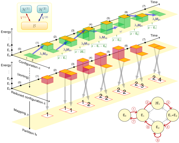
Figure 2: An example of a walk arising at 7th order perturbation theory $T_{7}=V_{-+}(G_{+}V_{+})^{5}G_{+}V_{+-}$. Top left: the specific physical setting concerned, where the number of subsystems is $m=2$. Top layer: the relationship between the 7-step walk in the space of energy configurations ${\bf c}$ and an upper bound associated with it. Each transition due to $V$ is associated with a factor of either $\lambda_{i}M_{st}$ or $\omega$. Each intermediate step with energy $E^{(i)}$ contributes a term ${1}/{|z-E^{(i)}|}$ due to $G_{+}$. Middle layer: the corresponding walk in $\tilde{\bf c}$, where at each step $\tilde{\bf c}^{(i)}$ is obtained by sorting ${\bf c}$ in descending order. Bottom layer: the corresponding change in the partition $\bf b$ and the mapping $\mu:\tilde{\bf c}\mapsto{\bf b}$ maintained throughout. By convention, the partition ${\bf b}$ is always of non-decreasing order. Bottom right: the walk in the space of energy combination ${\bf n}$ corresponding to the walk in $\tilde{\bf c}$. This walk in ${\bf n}$ is what the cellular automaton algorithm essentially implements.

The expressions for the upper bounds to $\|T_{r}\|_{\infty}$ such as on the right hand side of Equation 4 looks simple for $r=2$. At higher order, however, the situation quickly becomes more complicated. Intuitively this is because each unperturbed system has $\ell$ possible energy levels, and $m$ such subsystems could manifest $\ell^{m}$ possible ways in which the energies of each subsystems are assigned. Therefore any matrix element of $T_{r}$ should be a sum of roughly at most $O(\ell^{mr})$ walks, yielding an exponential complexity with respect to the total system size $m$. However, we note that such exponential complexity could be reduced to merely poly$(m)$ by exploiting the inherent permutation symmetry of upper bounds such as Equation 4. The essential observation is that these upper bounds are invariant with respect to permutation of the subsystems. This implies that they are symmetric functions over the $\lambda_{i}$ variables. In particular, these upper bounds to $\|T_{r}\|_{\infty}$ are linear combinations of monomial symmetric polynomials, which can be written in form of [11]

$$m_{\bf b}({\bm{\lambda}})=\sum_{\pi\in S_{k}}\lambda_{\pi(1)}^{b_{1}}\lambda_{\pi(2)}^{b_{2}}\cdots\lambda_{\pi(k)}^{b_{k}}$$

where ${\bf b\in\mathbb{N}^{k}}$ is a vector which we call partition, $\bm{\lambda}=(\lambda_{1},\cdots,\lambda_{m})$ and the summation is over a permutation group $S_{k}$, where any permutation $\pi$ chooses $k$ elements from $m$ elements and permutes them. For example, $m_{(1,2)}(\lambda_{1},\lambda_{2},\lambda_{3})=\lambda_{1}\lambda_{2}^{2}+\lambda_{1}\lambda_{3}^{2}+\lambda_{2}\lambda_{3}^{2}+\lambda_{2}\lambda_{1}^{2}+\lambda_{3}\lambda_{2}^{2}+\lambda_{3}\lambda_{1}^{2}$ is a monomial symmetric polynomial. Equation 4 could be compactly represented as $\|T_{2}\|_{\infty}\leq\frac{1}{|z-E_{1}|}M_{01}M_{10}m_{(2)}$. At $4$-th order we could show that

$$\|T_{4}\|_{\infty}\leq\displaystyle\frac{M_{01}M_{10}\omega^{2}m_{(2)}}{|(z-E_{1})^{3}|}+\frac{2M_{01}^{2}M_{10}^{2}m_{(2,2)}}{|(z-E_{1})^{2}(z-2E_{1})|}+\frac{M_{01}M_{12}M_{21}M_{10}m_{(4)}}{|(z-E_{1})^{2}(z-E_{2})|}.$$ (5)

By respecting the matrix product structure of $T_{r}$, the symmetric polynomial upper bounds such as those in Equations 4 and 5 turn out to be a much more accurate estimation of the true magnitude of $\|T_{r}\|_{\infty}$ than crude bounds using geometric series such as $\|T_{r}\|_{2}\leq\|V\|_{2}\cdot\|G_{++}\|_{2}\cdot\|V\|_{2}\cdots\|G_{++}\|_{2}\cdot\|V\|_{2}$. In later discussions we will demonstrate this point using numerical examples.

The question then becomes how we may assemble expressions such as (4) and (5) in an algorithmic fashion. We accomplish this efficiently by using cellular automata as the basic data structure. In a nutshell, a cellular automaton is a computational model consisting of a network of basic units called cells that are connected by directed edges. Each cell stores some data which represent its current state. All the cells are assigned an initial state and the computation proceeds by evolving each cell using an identical rule for updating its state. The new state of each cell is only dependent on the previous states of the same cell and its neighbors. The study of cellular automata dates back to the 1940s [12], followed by interesting constructions [13, 14, 15] and formal, systematic study over the past decades [16, 17]. Though computationally rich, the structure of cellular automata considered in these contexts are commonly rather simple, with cells that have discrete sets of possible states and are connected by simple network geometries (such as a 2D grid). In our case, as we will discuss later, the cells in cellular automata store more complex data structures and are connected with often non-planar network geometries. The update rules designed specifically so that the coordination of cells as a whole computes the symmetric polynomial upper bound for $\|T_{r}\|_{\infty}$.

The connection between cellular automata and perturbation theory seems unusual at first glance. However, the connection between cellular automata and random walks is well documented [18, 19, 20]. Such connection, combined with our earlier discussion on how the symmetric polynomial upper bounds could arise from summing over walks on the set of $H$ eigenstates, suggests that one may also be able to use cellular automata for the summation over these walks. One could further think of our task of computing a symmetric polynomial upper bound to $\|T_{r}\|_{\infty}$ as summing over walks in a space of energy configurations ${\bf c}$, which are $m$-dimensional vectors of indices ranging from $0$ to $\ell-1$ indicating the energy level of each subsystem in a particular $H$ eigenstate. In other words, ${\bf c}=(c_{1},\cdots,c_{m})\in\{0,1,\cdots,\ell-1\}^{m}$ and $\langle\phi|H^{(i)}|\phi\rangle=E_{c_{i}}$ for any particular $H$ eigenstate $|\phi\rangle$. Therefore each $r$-step walk in the space of $H$ eigenstates corresponds to a walk in the space of energy configuration ${\bf c}$, which is of size $O(\ell^{m})$. We could reduce the size of this space by taking every energy configuration ${\bf c}$ and sort its elements to produce a new vector $\tilde{\bf c}$, which we call reduced energy configuration. Like the number of energy levels in $H$, the set of $\tilde{\bf c}$ is also of size $O(m^{\ell})$, which is polynomial is $m$ assuming $\ell$ is a constant and intensive property of each subsystem (for instance a spin-1/2 particle has $\ell=2$ if we are only concerned with the spin degree of freedom). Each energy level of $H$ is a sum of the energies of the subsystems: $\langle\phi|H|\phi\rangle=\sum_{i=0}^{\ell-1}n_{i}E_{i}=E({\bf n})$ where $E_{i}$ is one of the $\ell$ possible energy levels of a subsystem. We could write each energy level of $H$ as an $\ell$-dimension vector ${\bf n}=(n_{0},n_{1},\cdots,n_{\ell-1})$ which we call energy combination (Figure 2 middle layer).

With the discussion so far we have reduced the problem of summing over walks on the set of $H$ eigenstates, whose number scales exponentially with respect to system size parameter $m$, to one that concerns only with walks on the set of ${\bf n}$, which is of only polynomial size in $m$. In accomplishing this reduction, we introduced the notion of energy configuration ${\bf c}$ and reduced energy configuration $\tilde{\bf c}$. Going from walks in ${\bf c}$ to $\tilde{\bf c}$ is a major step that takes advantage of the permutation symmetry with respect to the $m$ subsystems in the $r$-th order from $T_{r}$. We capture this symmetry with the use of symmetric polynomials $m_{\bf b}(\bm{\lambda})$. We illustrate this concept in Figure 2. We note that the partition ${\bf b}$ does not contain all of the information associated with a walk in $\tilde{\bf c}$. Consider a particular walk on the set of $H$ eigenstates and its associated weight whose functional form is shown in Equation 3, ${\bf b}$ only records the number of times that some subsystem is acted on by $V$, without the information about the order and the energies of the subsystem before and after the action (Figure 2 bottom layer). For example the partition $(1,2)$ means “one of the subsystems is acted on by $V$ once and another is acted on by $V$ twice”. The expression $m_{(1,2)}(\bm{\lambda})$ sums over the weights of walks that fits that description. But there are more than one possible walks, be it on the set of $H$ eigenstates or ${\bf c}$ or $\tilde{\bf c}$, that fits the description. Therefore in order for a symmetric polynomial to accurately represent an upper bound to the contributions to $\langle\phi|T_{r}|\phi^{\prime}\rangle$ from all walks in $\tilde{\bf c}$, a mapping must be maintained between ${\bf b}$ and $\tilde{\bf c}$ to indicate which subsystem is being acted on at the current step. Figure 2 shows an example that illustrates the connection between $\tilde{\bf c}$, ${\bf b}$, and $\mu$ to a walk in the configuration space ${\bf c}$.

In our construction cellular automata that executes the summation over walks in $\tilde{\bf c}$, each cell corresponds to an energy level of $H$. Hence there are in total $O(m^{\ell})$ cells. We use the energy combinations ${\bf n}$ to uniquely label each cell. Then the cells are connected with directed edges such that cell ${\bf n}$ will only be connected to cell ${\bf n}^{\prime}$ if there are eigenstates $|\phi\rangle$, $|\phi^{\prime}\rangle$ of $H$ with energy combinations ${\bf n}$ and ${\bf n}^{\prime}$ respectively such that $|\langle\phi|V|\phi^{\prime}\rangle|\neq 0$. In our algorithm each monomial symmetric polynomial $\xi m_{\bf b}(\bm{\lambda})$ is represented with a 4-tuple $(\tilde{\bf c},{\bf b},\xi,\mu)$ where $\xi$ is a scalar quantity indicating the weight of $m_{\bf b}(\bm{\lambda})$ in the overall symmetric polynomial upper bound. $\tilde{\bf c}$ and ${\bf b}$ are respectively the reduced energy configuration and partition at the current step of the walk. $\mu:\tilde{\bf c}\mapsto{\bf b}$ is a bijective mapping between $\tilde{\bf c}$ and ${\bf b}$, as justified in previous discussion.

Each cell of the automaton stores a list of 4-tuples $(\tilde{\bf c},{\bf b},\xi,\mu)$ as its state. As shown in Figure 4, at each iteration the state of each cell is updated in a two-phase process. In phase I (Figure 4a), the list of 4-tuples stored in $\mathcal{S}_{\bf n}$ is first merged with thosed stored in all of the incident edges to $\mathcal{S}_{\bf n}$ and then the coefficients of all the 4-tuples in $\mathcal{S}_{\bf n}$ are multiplied by a factor $1/|z-E({\bf n})|$. The intuition is that each 4-tuple corresponds to a particular walk such as the one shown in Figure 2. The multiplication by $1/|z-E({\bf n})|$ essentially accounts for the contribution from $G_{+}$ in $T_{r}$. In phase II, we account for the contribution from $V$ terms in $T_{r}$ by first computing new 4-tuples with $\tilde{\bf c}$ that can be generated from the current 4-tuples in $\mathcal{S}_{n}$ with one application of $V$, and then distributing the new 4-tuples among the outgoing edges $\mathcal{S}_{{\bf n},{\bf n}^{\prime\prime}}$, as shown in Figure 4b.

As the cells evolve, the 4-tuples are updated and passed along between the cells so that at the end of $r$ iterations, we could glean the symmetric polynomial upper bound from the states of the cells. The update rules for each cell are designed to maintain the property that at any iteration, each cell ${\bf n}$ contains a list of 4-tuples $(\tilde{\bf c},{\bf b},\xi,\mu)$ each of which corresponds to the set of all walks in $\tilde{\bf c}$ that leads up to a state with energy combination ${\bf n}$, and $\xi m_{\bf b}(\bm{\lambda})$ is an upper bound to the total contribution of the walks on the set of $H$ eigenstates that share the same corresponding walk in $\tilde{\bf c}$. In other words, $\xi m_{\bf b}(\bm{\lambda})$ is a sum of expressions such as Equation 3 for these walks on the set of $H$ eigenstates. We are able to rigorously show that with suitable initialization, after $r$ iterations the cellular automaton is indeed able to find a symmetric polynomial upper bound for $\|T_{r}\|_{\infty}$ similar to that of $\|T_{4}\|_{\infty}$ in Equation 5.

We stress that the overall time complexity of our algorithm scales polynomially as the system size grows. The degree of the polynomial, however, depends on the order of perturbation theory. For convergent series, the exponential dependence on the order $r$ of perturbation theory could be handled in practice by for instance setting a threshold $\eta$ such that when the symmetric polynomial upper bound computed by the cellular automaton is below $\eta$ at some order $r_{c}$ of perturbation, we bound the remaining terms up to infinity by a geometric series. For different problems and choices of $\eta$, the value of $r_{c}$ may vary. But the overall polynomial scaling with respect to the system size $m$ should not be affected.

   
   

In the mathematical developments of physical theories one is often concerned with the representation of the solution to a problem. For very few problems are we able to find a close-form, explicit formula as a representation of the solution. Series expansions are then introduced to largely enhance our ability to solve difficult problems far beyond analytical solution, as they allow for representation of a much wider class of mathematical objects. If we think of these representations as efficient procedures that allow us to construct our solution, then in greater generality we could argue that the outputs of efficient algorithms are also valid representations of our solution. Our scheme based on cellular automata essentially produces this type of representation: the symmetric polynomial upper bound to $\|T_{r}\|_{\infty}$ that we have devised is most conveniently expressed in form of an algorithmic output, rather its explicit self as a sum of monomials. A similar example to this situation is perhaps the development of tensor networks as representations for quantum ground states [21, 22, 23]. As is the case for our algorithmic development, tensor networks are also intended to cope with the exponential size of Hilbert space as the physical system grows. Using innovative data structures based on tensors, one obtains a polynomial size approximation to the true ground state. The resulting ground state is then most conveniently represented in form of a tensor network rather than its exponential-size self as a linear combination of basis states. Our cellular automaton algorithm could also be thought of as producing an approximation to $\|T_{r}\|_{\infty}$, in the sense that we replace the action of $V$ on the unperturbed eigenstates $|\phi\rangle$, $|\phi^{\prime}\rangle$ of each subsystem $i$ by scalar quantities $\lambda_{i}$ and $\omega$, and we use the integers $M_{st}$ to obtain a sketch of the structure of $V$. Such approximations may seem crude at first sight, but they preserve the combinatorial structure of $T_{r}$ as a matrix product, and allow for compact description using symmetric polynomials. We use iteration of cell evolution as a natural means to compute these symmetric polynomials. As a result, the output of our cellular automaton algorithm is the most natural representation for the upper bound to $\|T_{r}\|_{\infty}$ that we have devised.

One of the areas where our algorithm could find direct application is quantum computation. Though perturbation theory has been pervasively used for calculating properties of quantum systems, the lack of efficient and effective methods for estimating the error even for convergent series has cast a wide shadow of uncertainty on these calculations. Such problem becomes ever more imminent when one tries to engineer quantum systems that are intended to meet specific application requirements such as quantum computing [24, 25, 26]. As the implementations of quantum devices scale up and perturbation theory finds its inevitable use in analyzing these devices, it is imperative to have a scalable method for estimating the error in the perturbative expansion.

For example, in quantum simulation one often wishes to construct a two-body physical system $\tilde{H}$ whose low energy effective interactions $H_{\text{eff}}$ are many-body [9, 10, 27]. The most general construction of $\tilde{H}$ to date that could generate arbitrary many-body dynamics in $H_{\text{eff}}$ is based on perturbation theory. Here in Figure 3 we show one example of such construction with $H_{\text{eff}}=\alpha_{1}X_{1}X_{2}X_{3}+\alpha_{2}X_{2}Y_{4}Z_{5}$ being three-body while $\tilde{H}=H+V$ is entirely two-body [27]:

$$\begin{array}[]{ll}H=H^{(1)}+H^{(2)},&\displaystyle\qquad\qquad H^{(1)}=\frac{\Delta}{4}(Z_{u_{1}}Z_{u_{2}}+Z_{u_{2}}Z_{u_{3}}+Z_{u_{1}}Z_{u_{3}})\\[7.22743pt] &\displaystyle\qquad\qquad H^{(2)}=\frac{\Delta}{4}(Z_{v_{1}}Z_{v_{2}}+Z_{v_{2}}Z_{v_{3}}+Z_{v_{1}}Z_{v_{3}})\\[7.22743pt] V=V^{(1)}+V^{(2)},&\qquad\qquad V^{(1)}=\mu_{1}(X_{1}X_{u_{1}}+X_{2}X_{u_{2}}+X_{3}X_{u_{3}})\\[3.61371pt] &\qquad\qquad V^{(2)}=\mu_{2}(Y_{4}X_{v_{1}}+X_{2}X_{v_{2}}+Z_{5}X_{v_{3}})\end{array}$$ (6)

where spins with $u_{i}$ and $v_{i}$ labels belong to the two unperturbed subsystems. Here we let $\Delta$ be orders of magnitude larger than $\mu_{1}$ and $\mu_{2}$ and keep the coefficients $\mu_{1}$ and $\mu_{2}$ as $\mu_{1}=({\alpha_{1}\Delta^{2}}/{6})^{1/3},\mu_{2}=({\alpha_{2}\Delta^{2}}/{6})^{1/3}$. Perturbative calculation on $\tilde{H}$ show that the leading three orders $T_{1}+T_{2}+T_{3}=H_{\text{eff}}\otimes\Pi$ for some projector $\Pi$ acting on a Hilbert space separate from that of $H_{\text{eff}}$. The simulator Hamiltonian $\tilde{H}$ is constructed such that the perturbative series converges. In our example $\tilde{H}$ consists of only two-body spin interactions and parameters $\omega=0$, $\lambda_{1}=\mu_{1}$, $\lambda_{2}=\mu_{2}$ and $M_{st}$ can be computed from Figure 3d. The cellular automaton in this case is set up as in Figure 4. We then proceed to evolve the cellular automaton, gathering outputs from the cells corresponding to the low energy subspace. As shown in Figure 5, even with the convergence, simple geometric series upper bounds fail to capture the true magnitude of $\|T_{r}\|_{\infty}$ while the output of our cellular automaton algorithm is essentially tight with respect to the true value. Note that the true value takes an exponential amount of computational effort in $m$ while our cellular automaton algorithm costs only polynomial in $m$, as discussed before. This implies that we could obtain efficient and accurate estimations for the error of our quantum simulation that are not previously available.

Beyond quantum computing, our algorithm should retain its effectiveness for general spin systems and find its application in greater areas of condensed matter physics. For example, dimensional scaling method, pioneered by Herschbach [5], uses the inverse space dimensionality as a perturbation free parameter to solve complex many-body problems by taking the large-dimensional limit as the zeroth order approximation. At this limit many problems admit a simple solution, as in the electronic structure calculations of atoms and molecules. Moreover, the second-order term also can be calculated but the higher order terms are cumbersome and hard to estimate [5]. This new proposed algorithm might be useful to estimate the perturbation error in dimensional scaling method which will lead to a very powerful and efficient approach to solve complex many-body problems. Like tensor networks, which triggered an entirely new direction of research, it would be exciting to see what deeper truths of our quantum world could be unveiled by innovative proposals of algorithms and data structures.

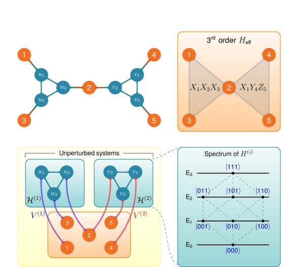
Figure 3: A numerical example for demonstrating our algorithm estimating the perturbative error. (a) The 11-spin system constructed for testing. Each node corresponds to a spin-1/2 particle and each edge represents an interaction term in the Hamiltonian between two spins. (b) Effective Hamiltonian truncating at 3rd order perturbation theory. Here each triangle represents a 3-body interaction term. Using the perturbative expansion in Equation 1 we could show that the low-energy effective Hamiltonian truncated at 3rd order is $H_{\text{eff}}=\alpha_{1}X_{1}X_{2}X_{3}+\alpha_{2}X_{2}Y_{4}Z_{5}$ up to a constant energy shift. (c) Rearranging and partitioning the system in (a) according to the setting of perturbation theory used. Here each unperturbed system $H^{(i)}$ consists of three ferromagnetically interacting spins (details in the long version). (d) Spectrum of each subsystem $H^{(i)}$ in (a), $i\in\{1,2\}$. Here each node represents an eigenstate of $H^{(i)}$. Nodes on a same horizontal dashed line belong to the same energy subspace $\mathcal{P}_{j}$. There is an edge $(u,v)$ iff $\|\langle u|V|v\rangle\|\neq 0$. For example, if we consider this diagram as representing $H^{(1)}$, since $V^{(1)}|001\rangle_{u_{1}u_{2}u_{3}}\propto(|101\rangle+|011\rangle+|000\rangle)_{u_{1}u_{2}u_{3}}$ we connect the $|001\rangle$ with the nodes representing $|101\rangle$, $|011\rangle$ and $|000\rangle$.

Figure 4: The cellular automaton generated for the example considered in Figure 3. Here each cell corresponds to an energy level of the unperturbed system $H=H^{(1)}+H^{(2)}$. The sets of 4-tuples $\mathcal{S}_{i}$ and $\mathcal{S}_{i,j}$ at each cell and each directed edge store lists of 4-tuples $(\tilde{\bf c},{\bf b},\xi,\mu)$. For details, refer to the long version. (a) and (b): Schematic diagrams for illustrating the two sequential steps executed when updating the state of each cell during an iteration. (c) A table listing the energy combinations ${\bf n}$, energy $E({\bf n})$ and the subspace (low energy $\mathcal{L}_{-}$ or high energy $\mathcal{L}_{+}$) associated with each cell. (d) The cellular automaton constructed for the example considered in Figure 3 and Equation 6. Here the dashed lines corresponds to edges that go from a node in $\mathcal{L}_{+}$ to one in $\mathcal{L}_{-}$, which is only present in the automaton during the final step.

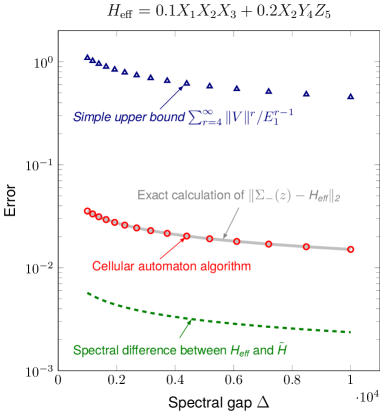
Figure 5: Comparison between the upper bounds computed using the cellular automaton algorithm and the norm computed using (inefficient) explicit method. The “actual spectral error” in this plot shows the maximum difference between the eigenvalues of $H_{\text{eff}}$ and their counterparts in $\tilde{H}$, which are the energies of its $2^{N}$ lowest eigenstates with $N=5$ being the number of particles that $H_{\text{eff}}$ acts on (Figure 3b). The actual spectral error is always lower than the error computed based on $\|\Sigma_{-}(z)-H_{\text{eff}}\|_{2}$ because $\|\Sigma_{-}(z)-H_{\text{eff}}\|_{2}\leq\epsilon$ is only a sufficient condition that guarantees the spectral difference between $\tilde{H}$ and $H_{\text{eff}}$ being within $\epsilon$ (see Theorem 1 of the long version).

See pages - of som

References

- [1] C. M. Bender and S. A. Orszag. Advanced Mathematical Methods for Scientists and Engineers I: Asympotic methods and perturbation theory. Springer Science & Business Media, 1999.
- [2] T. Helgaker, P. Jorgensen, and J. Olsen. Molecular Electronic-Structure Theory. Wiley, 2000.
- [3] A. Szabo and N. S. Ostlund. Modern Quantum Chemistry. Dover Publications, New York, 1996.
- [4] H. Primas. Generalized perturbation theory in operator form. Rev. Mod. Phys., 35(710), 1963.
- [5] D. R. Herschbach, J. S. Avery, and O. Goscinski. Dimensional scaling in chemical physics. Springer, Springer Netherlands, 1993.
- [6] S. Kais. Advances in Chemical Physics, Quantum Information and Computation for Chemistry, volume 154. John Wiley and Sons, New York, 2014.
- [7] M. J. Martin, M. Bishof, M. D. Swallows, X. Zhang, C. Benko, J. von Stecher, A. V. Gorshkov, A. M. Rey, and Jun Ye. A quantum many-body spin system in an optical lattice clock. Science, 341(6146):632–636, 2013.
- [8] R. Islam, C. Senko, W. C. Campbell, S. Korenblit, J. Smith, A. Lee, E. E. Edwards, C.-C. J. Wang, J. K. Freericks, and C. Monroe. Emergence and frustration of magnetism with variable-range interactions in a quantum simulator. Science, 340(6132):583–587, 2013.
- [9] J. Kempe, A. Kitaev, and O. Regev. The complexity of the Local Hamiltonian problem. SIAM J. Computing, 35(5):1070–1097, 2006.
- [10] R. Oliveira and B. Terhal. The complexity of quantum spin systems on a two-dimensional square lattice. Quant. Inf, Comp., 8(10):0900–0924, 2008.
- [11] I. G. MacDonald. Symmetric Functions and Hall Polynomials. Oxford University Press, Oxford, UK, 1998.
- [12] J. von Neumann. The general and logical theory of automata. Lecture, 1948. Pasadena, California.
- [13] N. Wiener and A. Rosenblueth. The mathematical formulation of the problem of conduction of connected excitable elements, specifically in cardiac muscle. Arch. Inst. Cardiol. Mex., 16(3):205–265, 1946.
- [14] M. Gardner. The fantastic combinations of John Conway’s new solitaire game “life”. Sci. Amer., 223:120–123, 1970.
- [15] A. R. Smith. Simple non-trivial self-reproducing machines. In C. G. Langton, C. Taylor, J. D. Farmer, and S. Rasmussen, editors, Artificial Life II, SFI studies in the Sciences of Complexity, volume X. Addison-Wesley, 1991.
- [16] C. E. Shannon. Von neumann’s contributions to automata theory. Bull. Amer. Math. Soc., 64:123–129, 1958.
- [17] S. Wolfram. Statistical mechanics of cellular automata. Rev. Mod. Phys., 55(3):601–644, 1983.
- [18] T. Toffoli and N. Margolus. Cellular Automata Machines: A New Environment for Modeling. MIT Press, Cambridge, Massachusetts, 1987.
- [19] E. Nummelin K. Eloranta. The kink of cellular automaton rule 18 performs a random walk. Journal of Statistical Physics, 69:1131–1136, 1992.
- [20] K Eloranta. Random walks in cellular automata. Nonlinearity, 6(6):1025, 1993.
- [21] F. Verstratete, J. I. Cirac, and V. Murg. Matrix product states, projected entangled pair states, and variational renormalization group methods for quantum spin systems. Adv. Phys., 57(143), 2008.
- [22] J. I. Cirac and F. Verstraete. Renormalization and tensor product states in spin chains and lattices. J. Phys. A: Math. Theor., 42(504004), 2009.
- [23] R. Augusiak, F. M. Cucchietti, and M. Lewenstein. Many-body physics from a quantum information perspective. In Daniel C. Cabra, Andreas Honecker, and Pierre Pujol, editors, Lecture notes in Physics, volume 843, chapter 6, pages 245–294. Springer-Verlag, Berlin Heidelberg, 2012.
- [24] S. Lloyd and B. Terhal. Adiabatic and Hamiltonian computing on a 2D lattice with simple 2-qubit interactions. New J. Phys., 18:023042, 2016.
- [25] Y. Cao, R. Babbush, J. Biamonte, and S. Kais. Hamiltonian gadgets with reduced resource requirements. Phys. Rev. A, 91(1):012315, 2015.
- [26] Y. Cao and D. Nagaj. Perturbative gadget without strong interactions. Quant. Info. Comput., 15(13, 14):1197–1222, 2014.
- [27] S. P. Jordan and E. Farhi. Perturbative gadgets at arbitrary orders. Phys. Rev. A, 77:062329, 2008.